Data-Agnostic Face Image Synthesis Detection Using Bayesian CNNs

Abstract

Face image synthesis detection is considerably gaining attention because of the potential negative impact on society that this type of synthetic data brings. In this paper, we propose a data-agnostic solution to detect the face image synthesis process. Specifically, our solution is based on an anomaly detection framework that requires only real data to learn the inference process. It is therefore data-agnostic in the sense that it requires no synthetic face images. The solution uses the posterior probability with respect to the reference data to determine if new samples are synthetic or not. Our evaluation results using different synthesizers show that our solution is very competitive against the state-of-the-art, which requires synthetic data for training.

Keywords Face synthesis  $\cdot$ Deep Fakes  $\cdot$ Agnostic Models  $\cdot$ Anomaly Detection  $\cdot$ Computer Security

1 Introduction

Face image-based technology is fast growing for many user authentication purposes [1] making it an essential component of several authentication systems. In this context, face image synthesis poses a problem for many user profile-based systems that rely on face images, e.g., the use of fake social media accounts to spread misinformation [2, 3] or the use of synthetic biometrics to commit identity fraud. State-of-the-art methods can generate high-quality face images with outstanding levels of featuring [4, 5]. Hence, it is important to accurately detect synthesized face images to reduce their negative impact on society.

Existing solutions to detect the face image synthesis process require, unfortunately, synthetic data at some point in the training process to learn to differentiate between real and synthetic face images. This is an important drawback because some models with undisclosed architectures can easily trick the detector by generating never-seen-before data that looks very realistic. In this paper, we present a solution based on the anomaly detection framework, which requires training a model only with real data to learn to identify one class. This solution is then data-agnostic in the sense that does not require any synthetic face images. Our contributions are as follows:

1. We use an anomaly detection framework to detect synthetic data, which departs from the trend to use 2-class classifiers.

2. Our proposed solution requires only real data to detect the synthesis process using a probabilistic approach.

3. Our solution achieves very competitive performance, outperforming several state-of-the-art solutions.

The rest of this paper is organized as follows. In Section 2, we review the most related work. In Section 4, we present the proposed solution. Section 5 provides experimental results and Section 6 concludes this paper.

2 Related Work

The majority of the work related to the detection of the face image synthesis process is also related to deepfake detection. Such detection methods require detecting the faces at some point in the process, as synthetic images usually depict artifacts in the depicted faces [6, 7]. For example, Afchar et al. [8] propose a Convolutional Neural Network (CNN)based on the InceptionV3 model [9] to detect synthetic face images in videos. Their method uses the Viola-Jones face detector followed by registration, alignment, and scaling. It detects the synthesis process frame-by-frame by giving a score to each frame depicting a face. Hsu et al. [10] propose a Generative Adversarial Network (GAN)-based solution that requires measuring the contrastive loss given by the GAN discriminator. Because their solution requires measuring the reconstruction error of the GAN, a secondary Support Vector Machine (SVM)is used to detect the synthesis process using the discriminator loss. Marra et al. [11] inspect a set of well-established generic models for image-related tasks, e.g. IV3, DenseNet, Xception, [9, 12, 13], to detect synthetic face images. Their work reveals that standard architectures are inherently structured to detect the synthesis process. Nataraj et al. [14] propose detecting synthetic face images by using a set of co-occurrence matrices prior to a CNN. The authors suggest that a more descriptive input space can be generated by a set of cascade filters to detect the synthesis process. Maiano et al. [15] train several existing CNN backbones to detect the synthesis process in several color spaces. Their results show that architectures are very sensitive to the color space used for detection. Rossler et al. [16] propose to perform a series of manipulations to obtain more synthetic face images to train models. These manipulations include blending, 3D distortion, texturization, and 2D wrapping. Zhang et al. [17] propose learning to detect the face image synthesis process by solving an image-to-image translation problem simulating artifacts. Their work, which uses a GAN, shows that synthetic samples comprise low-level features visible in the Fourier domain. A further analysis of several patches is used to find distinctive patterns, thus the detection is based on spotting several artifacts. Similar spectral analyses are proposed by Frank et al. [18] by analyzing the Discreet Cosine Transform (DCT). The idea is that some types of synthesis can be easily detected under a more descriptive spatial and frequency transformation. Tolosana et al. propose to detect the face image synthesis process by means of facial landmarks [19]. Their work suggests that separate fused models can detect the synthesis by separately analyzing several face components, e.g., the nose and eyes. This methodology is also supported by the fact that some synthesizers can only replace part of the face instead of generating a whole new face [20]. Local and global matching is also explored by Favorskaya et al. [21]; however, their method heavily relies on additional features, e.g., those extracted from the background and areas surrounding the face. Fusing models to detect the synthesis process in videos is explored by Coccomini et al. Their method requires analyzing the faces frame by frame. It combines a CNN and the recently proposed Vision Transformer [22]. Wang et al. [23] propose a CNN to detect synthetic images in general. However, their work can also be used to detect synthetic face images. Other recent work [24] suggests adding artificially generated artifacts and then proceeding to detect the synthetic faces.

As discussed in this section, existing CNN architectures are well-suited to detect the face image synthesis process [8, 11, 23, 14]. However, they should be designed to capture the fine details of the face, which usually depict imperfections and artifacts associated with the synthesis process [19, 20, 21]. To this end, we design our solution using such standard CNN architectures while making sure to preserve the fine details of face images. However, differently from most common solutions, we use an anomaly detection framework.

3 The Proposed Solution

4 The Proposed Solution

Although strictly speaking the face image synthesis detection task is a binary classification problem aimed to determine whether a face image is real or synthetic, we assume that we have no information about the synthesizer. This is particularly useful when the attacker, who aims at synthesizing face images with malicious intentions, does not publicly disclose their model. Our proposed solution then aims at detecting synthetic face images without requiring any synthetic samples from any synthesizer at any stage. To this end, we use an anomaly detection framework. Although the anomaly detection framework is a well-known method, it has not been fully exploited for the detection of the face image synthesis process. Although the work in [24] also uses a one-class classifier within the context of anomaly detection, it relies on a set of local image perturbations added to real images to detect synthetic images using anomaly scores. Our work differs from that approach as it relies on a model that uses only one class with no perturbations to maximize the Maximum A posterior Probability (MAP), i.e., the probability of observing the samples. In this context, samples that do not fit the positive class (normal) are deemed to be part of the negative class (abnormal) [25]. To this end, we train a model exclusively with real face images and without the need to add any perturbations to the real data. We then use the trained model with never-seen-before samples from both classes, i.e., real and synthetic images. Our solution uses a fine-to-coarse Bayesian CNN, i.e., a set of convolutional layers followed by a Bayesian model implemented by Fully Connected (FC)layers. Bayesian models have recently been shown to be robust to overfitting and can effectively solve problems related to sub-parametrization [26]. Because we are only modeling one class, Bayesian models are then very convenient for this task.

Formally, let us define a set of images organized as the design matrix $X=\{x_{1},x_{2},\ldots x_{N}\}$. Let us use define a neural network with $L$ FC layers and output $y$ as follows:

$$y=f^{L}(w^{L},\ldots f(w^{L-1},\ldots(f^{1}(w^{1},z)))),$$ (1)

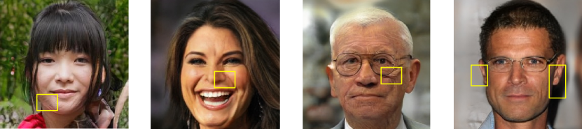
Figure 1: Sample artifacts in synthetic face images (left to right). Woman with ripples close to the chin, woman with unpaired nostril, man with scar below his left eye, and man with uneven ears.

Table 1: Architecture of the proposed fine-to-coarse Bayesian CNN.

Layer Type	Number of Filters	Feature Map Size	Kernel Size	Stride
Input		$256^{2}\times 3$
Center-Crop		$224^{2}\times 3$
RGB-normalization		$224^{2}\times 3$
Convolution Layer 1st	$16$	$224^{2}\times 16$	$5\times 5$	$1\times 1$
Mean Pooling Layer 1st			$4\times 4$	$2\times 2$
Sigmoid activation
Convolution Layer 2nd	$24$	$106^{2}\times 24$	$5\times 5$	$1\times 1$
Mean Pooling Layer 1nd			$4\times 4$	$2\times 2$
Sigmoid activation
Convolution Layer 3th	$32$	$50^{2}\times 32$	$5\times 5$	$1\times 1$
Mean Pooling Layer 1th			$4\times 4$	$2\times 2$
Sigmoid activation
Batch Normalization		$22^{2}\times 32\rightarrow 22^{2}\times 32$
Fully Connected Layer 1st		$22^{2}\times 32\rightarrow 512$
Dropout
Fully Connected Layer 2nd		$512\rightarrow 1$

where $f^{l}(w^{l},z)$ denotes the mapping function at layer $l$ with parameters $w^{l}$, and $z\in\mathrm{R}^{d}$ represents the latent feature space generated by a set of convolutional layers. The objective is then to train the Bayesian model that approximates $w^{l}$ for each FC layer $l$ by using the set of probabilistic parameters, $\theta=\{\alpha,\beta\}$, representing the mean and variance, respectively. The output $y$ can then be modeled as the conditional Gaussian distribution $p(y|z)$ with inverse variance $\beta^{-1}$:

$$p(y|z,w,\beta)=\mathcal{N}\left(y|f(z,w),\beta^{-1}\right)$$ (2)

where $p(w,\alpha)=\mathcal{N}(w|0,\alpha^{-1}\mathbf{I})$, with $\mathbf{I}$ as the identity matrix. For $N$ observations in $X$ with target values $\mathcal{D}=\{y_{1},y_{2},\ldots y_{N}\}$, the likelihood function is:

$$p(\mathcal{D}|w,\beta)=\prod\limits_{n=1}^{N}\mathcal{N}(y_{n}|f(z_{n},w),\beta^{-1}).$$ (3)

The desired posterior distribution is then:

$$p(w|\mathcal{D},\alpha,\beta)\approx p(w|\alpha)~{}p(\mathcal{D}|w,\beta).$$ (4)

It can be proved [27] that the parameter set given by the MAP is as follows:

$$p(y|z,\mathcal{D},w,\beta)=\mathcal{N}\left(y|f(z,w_{\mathrm{MAP}}),\sigma^{2}(z)\right),$$ (5)

where the input-dependent variance $\sigma$ is given by:

$$\sigma^{2}(z)=\beta^{-1}+g^{\top}(\alpha~{}\mathbf{I}+\beta~{}\mathbf{H})^{-1}g,$$ (6a)

$$g=\nabla_{w}y(z~{}|~{}w)\big{|}_{w=w_{\mathrm{MAP}}},$$ (6b)

where $\mathbf{H}$ is the Hessian matrix comprising the second derivatives of the sum of square errors with respect to the components of $w$. The distribution $p(y~{}|z,\mathcal{D})$ is Gaussian whose means are given by the network mapping function $f(w_{\mathrm{MAP}},z)$ and maximizes the posterior likelihood. To classify a sample $x$ as synthetic we can then use a threshold $\gamma$ on the posterior :

(a) XL-GAN samples

(b) DDPM samples

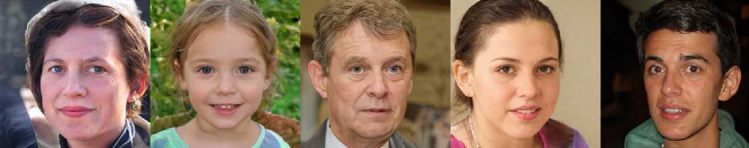
(c) InsGen samples

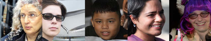
(d) SGAN 2 samples

Figure 2: Example of the synthetic face images generated by the synthesizers.

$$\gamma<f(w,x).$$ (7)

under the assumption that the posterior for real images is greater than that for synthetic images:

$$f(w,x_{\mathrm{~{}REAL}})>f(w,x_{\mathrm{~{}FAKE}}).$$ (8)

where $x_{\mathrm{~{}REAL}}$ is a real face image sample and $x_{\mathrm{~{}FAKE}}$ a synthetic one. Note that Eq. 8 is the foundation of the anomaly detection framework. In this work, we select the threshold $\gamma$ by inspecting the posteriors of real samples after training, which may cause the threshold to vary based on the model’s initial set of learnable parameters.

4.1 Fine-to-coarse Bayesian CNN

As suggested in [17], detecting synthetic face images can be effectively performed by detecting small visual imperfections and artifacts, e.g., unexpected wrinkles, scars, and small deformations. Fig. 1 shows several synthetic face images with visible artifacts. One can see that the synthesis process can indeed produce visible imperfections in the form of distortions or unusual human trait formations. Because we are interested in expanding the spatial information extracted from the images, our fine-to-coarse Bayesian CNN progressively increases the number of filters along the convolutions layers before feeding the extracted features to the FC layers. Furthermore, to minimize the information loss in the pooling stages, we employ mean pooling operations to reduce the loss of important visual details, especially the artifacts in synthetic face images, which tend to be quite small. Table 1 summarizes the architecture of the proposed fine-to-coarse Bayesian CNN. Note that the two FC layers form a Multi-Layer Perceptron (MLP)structure as the decision layers and constitute the Bayesian model. To produce large positive output values, we employ the Sigmoid activation function for all feature maps. Thus, the MLP receives only positive values.

5 Experiments

We perform experiments using the face image datasets Flick Faces High Quality (FFHQ) and CelebFaces Attributes Dataset (CELEBA) [28, 29], which comprise 70K and 30K real face image samples, respectively. Let us recall that our solution only requires real samples for training. However, to evaluate performance in detecting synthetic face images, we use four synthesizers to generate several synthetic face images. Specifically, we use the pre-trained models provided by the authors of these four synthesizers: SGAN 2 [30], XL-GAN [31], InsGen [32], and Denoising Diffusion Probabilistic Models (DDPM)[33] . Fig. 2 shows several samples generated by these four synthesizers. To have synthetic samples for evaluation along with the real samples in the FFHQ dataset, we generate 224K synthetic images, 56K generated by each of the four synthesizers. All 224K synthetic images are the same size as the real images in the FFHQ dataset and are in an uncompressed format. For the case of the CELEBA dataset, we generate 72K synthetic images to be used for evaluation along with the real samples, 24K synthetic images generated by each of the four synthesizers. All 72K synthetic images are the same size as the real images in the CELEBA dataset and are in an uncompressed format.

Table 2: mAp values ($\uparrow$) of several solutions for different synthesizers and split values for the FFHQ dataset. The best (second best) results are highlighted in bold (underlined).

Method	Synthesizer	Split (% of data used for training )
		20%	40%	60%	80%
DCT-Ridge [18]	SGAN 2 [30]	0.492	0.533	0.654	0.761
	InsGen [32]	0.501	0.534	0.583	0.741
	DDPM [33]	0.505	0.512	0.559	0.721
	XL-GAN [31]	0.511	0.522	0.544	0.698
DF [15]	SGAN 2	0.503	0.575	0.701	0.816
	InsGen	0.551	0.584	0.731	0.802
	XL-GAN	0.565	0.566	0.624	0.732
	DDPM	0.518	0.563	0.691	0.791
AutoGAN [17]	SGAN 2	0.513	0.544	0.603	0.729
	InsGen	0.544	0.576	0.623	0.787
	DDPM	0.512	0.525	0.557	0.653
	XL-GAN	0.504	0.518	0.544	0.642
BayesianCNN	SGAN 2	0.629	0.683	0.754	0.843
	InsGen	0.552	0.593	0.643	0.771
	DDPM	0.562	0.595	0.667	0.783
	XL-GAN	0.573	0.597	0.643	0.793

Table 3: mAp values ($\uparrow$) of several solutions for different synthesizers and split values for the CELEBA dataset. The best (second best) results are highlighted in bold (underlined).

Method	Synthesizer	Split (% of data used for training )
		20%	40%	60%	80%
DCT-Ridge [18]	SGAN 2 [30]	0.562	0.593	0.681	0.813
	DDPM [33]	0.578	0.594	0.615	0.794
	XL-GAN [31]	0.566	0.573	0.602	0.778
DF [15]	SGAN 2	0.552	0.642	0.770	0.833
	DDPM	0.575	0.654	0.723	0.805
	XL-GAN	0.602	0.614	0.693	0.791
AutoGAN [17]	SGAN 2	0.562	0.612	0.669	0.802
	DDPM	0.570	0.593	0.653	0.733
	XL-GAN	0.562	0.587	0.644	0.702
BayesianCNN	SGAN 2	0.664	0.743	0.773	0.843
	DDPM	0.602	0.655	0.694	0.796
	XL-GAN	0.632	0.667	0.730	0.812

Our fine-to-course Bayesian CNN is implemented in pyro using two GTX 1080 TI GPUs. We use an exponential learning rate scheduler having Stochastic Gradient Descent (SGD)as the backbone starting at $10^{-3}$ with a decay factor of $0.1$. We use a TraceGraph Evidence LOwer BOund (ELBO)loss function as a back-propagator and monitor the loss plateau on the validation and training sets. Initially, we use $50$ epochs and when the model achieves a 1% improvement in accuracy with respect to the previous validation iteration, we use it as the best model and continue iterating. Thus at the end of the training process, the best model is the one that achieves the best accuracy on the validation set. To prevent overfitting, we have an early stop criterion of $6\%$ between the accuracy achieved on the test set and the accuracy achieved on the validation set. The convolution banks are preset with Xavier initialization. We use batches of $5122$ samples.

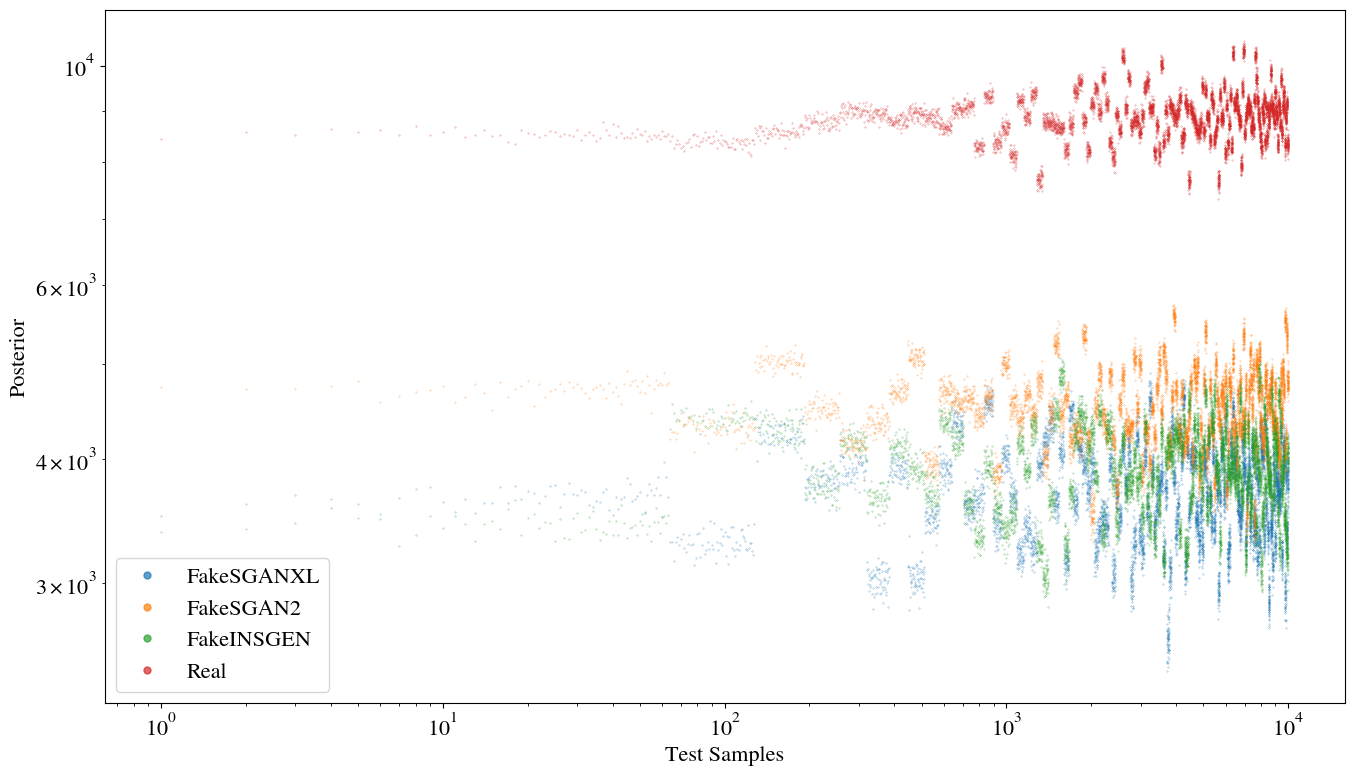
Figure 3: Posterior values produced by the proposed Bayesian CNN. The real and synthetic samples form two distinct regions. Thus, we can set the posterior threshold accordingly.

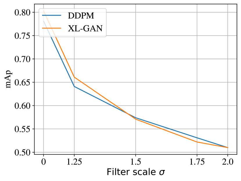
(a) Blurring.

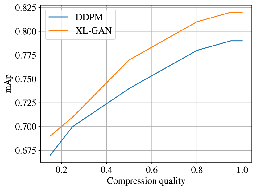
(b) JPEG compression.

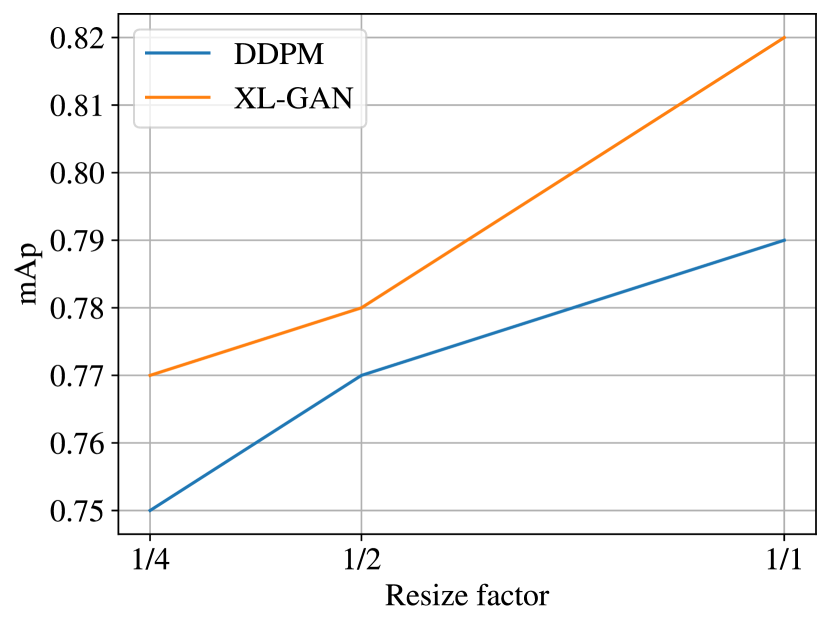
(c) Resizing.

Figure 4: Performance or the proposed solution when post-processing is used on the test images.

To make comparisons with existing methods, we use a similar strategy as that suggested by Gragnaniello et al. [34], which is a strategy for synthetic images in general, not exclusively face images. Their strategy requires training on a reference dataset targeting one class out of ten and testing on different image scales. Their strategy uses seven synthesizers to generate around 39K synthetic samples in an imbalanced fashion; i.e., more samples from some synthesizers than others. In this work, we are interested only in evaluating the capacity to detect synthetic face images regardless of the image scale. We then focus on evaluating the detection of unseen samples at one scale with balanced data generated by four synthesizers.

We compare our solution against the methods proposed in [18, 17, 15]. These methods are trained to detect real samples as the class $1$ and the synthetic samples as the class $0$. Specifically, we train these methods with a proportion of the real samples defined by the split used plus the same number of synthetic samples generated by one of the four synthesizers. We then use unseen data for testing, which includes the same proportion of unseen real samples and unseen synthetic samples. We repeat this process with both datasets and the other synthesizers. To compare against the method in [15], we only use the RGB color space.

For the method in [17] , we keep all the default settings from the implementation and only append the tree structure of the real/synthetic faces. No threshold is set to detect synthetic face images but only the output of the discriminator. For the method in [15], we train from zero a model using the reported parameters and set the classification threshold at $0.7$ from the last decision layer as it is not specified by the authors. We also add Sigmoid activations as the authors report the use of a binary cross entropy loss. For the method in [18], we employ a grid search to find the best parameters as the authors report for the described CNN. We set a classification threshold at $0.9$ that empirically provides good results. For our solution, we maximize the MAP until a plateau is observed. We set the threshold $\gamma$ in Eq. 7 after inspecting a few samples from the posterior distribution. In this case, the test samples are deemed real/synthetic after manually inspecting the validation set. Because the means and variances of the model are randomly initialized, we observe that the threshold should change for every run. The reported results in Tables 2 and 3 then use a different threshold for each split.

Table 2 and 3 tabulate results for the real images of the FFHQ dataset and the CELEBA dataset, respectively, in terms of the mean Average precision (mAp)values for different proportions (splits) of training data. In both tables, the tabulated splits indicate the proportion of real samples from each dataset used for training our solution. For the case of the other evaluated methods, the tabulated splits indicate the proportion of real samples from each dataset used for training plus the same amount of training synthetic samples generated by the synthesizer tabulated in each row. From Table 2, we can see that the proposed solution (BayesianCNN) achieves very competitive performance when trained on the real images of the FFHQ dataset. Particularly, using 80% of the available training data gives the best mAp values for two of the synthesizers. One can also see in Table 3 that the proposed solution also achieves very competitive performance when trained on the real images of the CELEBA dataset. Namely, our solution gives the best performance for the detection of synthetic images generated by the XL-GAN and SGAN 2 synthesizers.

We also examine the posteriors of the data generated by each synthesizer and plot them along with the posteriors of the real data in Fig. 3. This plot shows that it is indeed possible to distinguish the synthetic samples from the real ones by thresholding the posterior linearly. Hence, the threshold selection in Eq. 7 is appropriate as this establishes a linear margin. As we can see from this figure, the synthetic data is concentrated in a region where low posterior values exist. This further confirms that using an anomaly detection framework is an effective solution to detect synthetic face images. Moreover, such posterior values are intrinsic to our Bayesian CNN, which is expected to produce high posterior values for data that is very similar to the one used during training (i.e., real face images) and low values for never-seen data (i.e., synthetic face images). It is important to recall that the location of the region where the synthetic samples lie varies depending on the initialization of the model’s parameters.

We also evaluate performance after applying common post-processing on the test images: (1) Blurring by varying the size of the filter scale $\sigma$; (2) JPEG compression at different qualities; and (3) resizing by a factor of $1/2$ and $1/4$ using bilinear interpolation. Fig. 4 shows the results of this experiment. Fig. 4(a) shows that blurring has a very negative effect on performance, to the point of almost random classification for large values of $\sigma$. Fig. 4(b) shows that very aggressive compression hinders performance, yet the effect is not as severe as the one introduced by blurring the images. Finally, Fig. 4(c) has also a drastic effect, similar to blurring, as losing spatial information hinders the model’s performance in detecting the synthetic samples. This experiment reveals that the proposed solution is very sensitive to losing the fine details of the images as our Bayesian CNN relies on detecting such small artifacts and imperfections.

Finally, we also discuss several architectural decisions that led to the final architecture of our fine-to-coarse Bayesian CNN. We observe that small kernel sizes for the convolutional layers significantly improve the performance, e.g. $3-4\%$ on the large splits, while more than three filter banks have little effect on the performance but a severe impact on processing times. Compared to using filter banks of the same size, the proposed fine-to-coarse filter bank provides $5\%$ improvement on the large splits. We observe that more than two FC layers provide no significant improvement. Adding batch normalization provides faster convergence and less sensitivity to initialization. Finally, we observe that using dropouts, high posteriors can be achieved with significantly fewer parameters. Because our ultimate goal is to maximize the posterior for the real data with the fewest parameters possible, dropout is used. The proposed architecture in Table 1 then fairly trades performance for complexity.

6 Conclusion

In this paper, we have proposed a solution based on anomaly detection to detect synthetic face images, which implies training using only one class. Our solution is then data-agnostic as it requires no synthetic samples during training. This is a powerful advantage as we may not have information about the synthesizer or any of the synthetic face images. For detection, the solution uses a Bayesian CNN that extracts spatial features from the face images while preserving the small details associated with common artifacts and imperfections found in synthetic face images. Our performance evaluation results show that the proposed solution can achieve very competitive accuracy, outperforming several state-of-the-art methods that require training on real and synthetic face images. Our future work focuses on improving detection accuracy especially when post-processing is used on the test images, defining an automatic margin selection process to set thresholds, and conducting cross-data validations on more real/synthetic datasets.

References

- [1] Luca Maiano, Antonio Montuschi, Marta Caserio, Egon Ferri, Federico Kieffer, Chiara Germanò, Lorenzo Baiocco, Lorenzo Ricciardi Celsi, Irene Amerini, and Aris Anagnostopoulos. A deep-learning–based antifraud system for car-insurance claims. Expert Systems with Applications, page 120644, 2023.
- [2] Weihao Xia, Yulun Zhang, Yujiu Yang, Jing-Hao Xue, Bolei Zhou, and Ming-Hsuan Yang. Gan inversion: A survey. IEEE Transactions on Pattern Analysis and Machine Intelligence, 2022.
- [3] Irene Amerini, Mauro Conti, Pietro Giacomazzi, and Luca Pajola. Prana: Prnu-based technique to tell real and deepfake videos apart. In 2022 International Joint Conference on Neural Networks (IJCNN), pages 1–7, 2022.
- [4] Guodong Guo and Na Zhang. A survey on deep learning based face recognition. Computer Vision and Image Understanding, 189:102805, 2019.
- [5] Arash Vahdat and Jan Kautz. Nvae: A deep hierarchical variational autoencoder. Advances in Neural Information Processing Systems, 33:19667–19679, 2020.
- [6] Ali Khodabakhsh, Raghavendra Ramachandra, Kiran Raja, Pankaj Wasnik, and Christoph Busch. Fake face detection methods: Can they be generalized? In 2018 International Conference of the Biometrics Special Interest Group (BIOSIG), pages 1–6, Sep. 2018.
- [7] Roberto Leyva, Gregory Epiphaniou, Carsten Maple, and Victor Sanchez. Unsupervised face synthesis based on human traits. In 2023 11th International Workshop on Biometrics and Forensics (IWBF), pages 1–6, 2023.
- [8] Darius Afchar, Vincent Nozick, Junichi Yamagishi, and Isao Echizen. Mesonet: a compact facial video forgery detection network. In 2018 IEEE international workshop on information forensics and security (WIFS), pages 1–7. IEEE, 2018.
- [9] Christian Szegedy, Vincent Vanhoucke, Sergey Ioffe, Jon Shlens, and Zbigniew Wojna. Rethinking the inception architecture for computer vision. In Proceedings of the IEEE conference on computer vision and pattern recognition, pages 2818–2826, 2016.
- [10] Chih-Chung Hsu, Chia-Yen Lee, and Yi-Xiu Zhuang. Learning to detect fake face images in the wild. In 2018 international symposium on computer, consumer and control (IS3C), pages 388–391. IEEE, 2018.
- [11] Francesco Marra, Diego Gragnaniello, Davide Cozzolino, and Luisa Verdoliva. Detection of gan-generated fake images over social networks. In 2018 IEEE conference on multimedia information processing and retrieval (MIPR), pages 384–389. IEEE, 2018.
- [12] Gao Huang, Zhuang Liu, Laurens Van Der Maaten, and Kilian Q Weinberger. Densely connected convolutional networks. In Proceedings of the IEEE conference on computer vision and pattern recognition, pages 4700–4708, 2017.
- [13] François Chollet. Xception: Deep learning with depthwise separable convolutions. In Proceedings of the IEEE conference on computer vision and pattern recognition, pages 1251–1258, 2017.
- [14] Lakshmanan Nataraj, Tajuddin Manhar Mohammed, Shivkumar Chandrasekaran, Arjuna Flenner, Jawadul H Bappy, Amit K Roy-Chowdhury, and BS Manjunath. Detecting gan generated fake images using co-occurrence matrices. arXiv preprint arXiv:1903.06836, 2019.
- [15] Luca Maiano, Lorenzo Papa, Ketbjano Vocaj, and Irene Amerini. Depthfake: a depth-based strategy for detecting deepfake videos. arXiv preprint arXiv:2208.11074, 2022.
- [16] Andreas Rossler, Davide Cozzolino, Luisa Verdoliva, Christian Riess, Justus Thies, and Matthias Nießner. Faceforensics++: Learning to detect manipulated facial images. In Proceedings of the IEEE/CVF international conference on computer vision, pages 1–11, 2019.
- [17] Xu Zhang, Svebor Karaman, and Shih-Fu Chang. Detecting and simulating artifacts in gan fake images. In 2019 IEEE international workshop on information forensics and security (WIFS), pages 1–6. IEEE, 2019.
- [18] Joel Frank, Thorsten Eisenhofer, Lea Schönherr, Asja Fischer, Dorothea Kolossa, and Thorsten Holz. Leveraging frequency analysis for deep fake image recognition. In International conference on machine learning, pages 3247–3258. PMLR, 2020.
- [19] Ruben Tolosana, Sergio Romero-Tapiador, Julian Fierrez, and Ruben Vera-Rodriguez. Deepfakes evolution: Analysis of facial regions and fake detection performance. In Pattern Recognition. ICPR International Workshops and Challenges: Virtual Event, January 10–15, 2021, Proceedings, Part V, pages 442–456. Springer, 2021.
- [20] Ruben Tolosana, Ruben Vera-Rodriguez, Julian Fierrez, Aythami Morales, and Javier Ortega-Garcia. Deepfakes and beyond: A survey of face manipulation and fake detection. Information Fusion, 64:131–148, 2020.
- [21] Margarita Favorskaya and Anton Yakimchuk. Fake face image detection using deep learning-based local and global matching. CEUR Workshop Proceedings, 2021.
- [22] Alexey Dosovitskiy, Lucas Beyer, Alexander Kolesnikov, Dirk Weissenborn, Xiaohua Zhai, Thomas Unterthiner, Mostafa Dehghani, Matthias Minderer, Georg Heigold, Sylvain Gelly, et al. An image is worth 16x16 words: Transformers for image recognition at scale. arXiv preprint arXiv:2010.11929, 2020.
- [23] Sheng-Yu Wang, Oliver Wang, Richard Zhang, Andrew Owens, and Alexei A. Efros. Cnn-generated images are surprisingly easy to spot… for now. In Proceedings of the IEEE/CVF Conference on Computer Vision and Pattern Recognition (CVPR), pages 0–0, June 2020.
- [24] Nicolas Larue, Ngoc-Son Vu, Vitomir Struc, Peter Peer, and Vassilis Christophides. Seeable: Soft discrepancies and bounded contrastive learning for exposing deepfakes. In Proceedings of the IEEE/CVF International Conference on Computer Vision, pages 21011–21021, 2023.
- [25] R. Leyva, V. Sanchez, and C. T. Li. Video anomaly detection with compact feature sets for online performance. IEEE Transactions on Image Processing, 26(7):3463–3478, July 2017.
- [26] Sanae Lotfi, Pavel Izmailov, Gregory Benton, Micah Goldblum, and Andrew Gordon Wilson. Bayesian model selection, the marginal likelihood, and generalization. In International Conference on Machine Learning, pages 14223–14247. PMLR, 2022.
- [27] Christopher M Bishop and Nasser M Nasrabadi. Pattern recognition and machine learning, volume 4. Springer, 2006.
- [28] Tero Karras, Timo Aila, Samuli Laine, and Jaakko Lehtinen. Progressive growing of gans for improved quality, stability, and variation. arXiv preprint arXiv:1710.10196, 2017.
- [29] Ziwei Liu, Ping Luo, Xiaogang Wang, and Xiaoou Tang. Deep learning face attributes in the wild. In 2015 IEEE International Conference on Computer Vision (ICCV), pages 3730–3738, 2015.
- [30] Tero Karras, Samuli Laine, and Timo Aila. A style-based generator architecture for generative adversarial networks. IEEE Transactions on Pattern Analysis and Machine Intelligence, pages 1–1, 2020.
- [31] Axel Sauer, Katja Schwarz, and Andreas Geiger. Stylegan-xl: Scaling stylegan to large diverse datasets. In ACM SIGGRAPH 2022 conference proceedings, pages 1–10, 2022.
- [32] Ceyuan Yang, Yujun Shen, Yinghao Xu, and Bolei Zhou. Data-efficient instance generation from instance discrimination. Advances in Neural Information Processing Systems, 34:9378–9390, 2021.
- [33] Jonathan Ho, Ajay Jain, and Pieter Abbeel. Denoising diffusion probabilistic models. In H. Larochelle, M. Ranzato, R. Hadsell, M. F. Balcan, and H. Lin, editors, Advances in Neural Information Processing Systems, volume 33, pages 6840–6851. Curran Associates, Inc., 2020.
- [34] D. Gragnaniello, D. Cozzolino, F. Marra, G. Poggi, and L. Verdoliva. Are gan generated images easy to detect? a critical analysis of the state-of-the-art. In 2021 IEEE International Conference on Multimedia and Expo (ICME), pages 1–6, 2021.