The origin of the H$\alpha$ line profiles in simulated disc galaxies

Abstract

Observations of ionised H$\alpha$ gas in disc galaxies with high star formation rates have ubiquitous and significant line broadening with widths $\sigma_{\rm H\alpha}\gtrsim 50-100\,{\rm km\,s^{-1}}$. To understand whether this broadening reflects gas turbulence within the interstellar medium (ISM) of galactic discs, or arises from off-the-plane emission in mass-loaded galactic winds, we perform radiation hydrodynamic (RHD) simulations of isolated Milky Way-mass disc galaxies in a gas-poor (low-redshift) and gas rich (high-redshift) condition and create mock H$\alpha$ emission line profiles. We find that the vast majority of the ${\rm H\alpha}$ emission is confined within the ISM, with extraplanar gas contributing mainly to the extended profile wings. This substantiates the ${\rm H\alpha}$ emission line as a tracer of mid-plane disc dynamics. We investigate the relative contribution of diffuse and dense ${\rm H\alpha}$ emitting gas, corresponding to DIG ($\rho\lesssim 0.1\,{\rm cm^{-3}}$, $T\sim 8\,000$ K) and HII regions ($\rho\gtrsim 10\,{\rm cm^{-3}}$, $T\sim 10\,000$ K), respectively, and find that DIG contributes $\lesssim 10\,\%$ of the total L_Hα. However, the DIG can reach upwards of $\sigma_{\rm H\alpha}\sim 60-80\,{\rm km\,s^{-1}}$ while the HII regions are much less turbulent $\sigma_{\rm H\alpha}\sim 10-40\,{\rm km\,s^{-1}}$. This implies that the $\sigma_{\rm H\alpha}$ observed using the full ${\rm H\alpha}$ emission line is dependent on the relative ${\rm H\alpha}$ contribution from DIG/HII regions and a larger $f_{\rm DIG}$ would shift $\sigma_{\rm H\alpha}$ to higher values. Finally, we show that $\sigma_{\rm H\alpha}$ evolves, in both the DIG and HII regions, with the galaxy gas fraction. Our high-redshift equivalent galaxy is roughly twice as turbulent, except for in the DIG which has a more shallow evolution.

1 Introduction

The gas inside galactic discs, the interstellar medium (ISM), consist of various gas phases spanning several order of magnitude of densities and temperatures, from dense molecular clouds, where stars are formed, to warm ionised gas, which makes up a majority of the total gas volume but only a fraction of the mass (McKee & Ostriker, 1977). In particular, the ionised gas phase is prominent in the disc, outflows and extraplanar gas (Mac Low & Klessen, 2004; Haffner et al., 2009), and has several formation channels, e.g. ionising radiation from massive stars, supernovae shock winds, strong stellar winds, black hole feedback (Mac Low & Klessen, 2004; Haffner et al., 2009; Heckman & Best, 2014; Somerville & Davé, 2015). The nature and formation of these gas phases is not fully understood and is relevant for the reprocessing of gas between phases, but also for observations which use emission lines that trace ionised gas in order to interpret the dynamics and physical state of galaxies.

A prominent difference between gas phases is their kinematics. Gas turbulence, often quantified as the velocity dispersion $\sigma_{\rm g}$, is a fundamental property of galactic discs, with supersonic motions driving crucial physical processes such as star formation (Larson, 1981; Mac Low & Klessen, 2004; Renaud et al., 2012; Federrath, 2018), metal mixing (Yang & Krumholz, 2012; Armillotta et al., 2018), and density distributions (McKee & Ostriker, 2007). The ionised gas in local galaxies has been observed to be more turbulent, $\sigma_{\rm g}$ $\sim 15-30$${\,\rm{km\,s^{-1}}}$, (Epinat et al., 2010; Moiseev et al., 2015; Green et al., 2014; Varidel et al., 2016; Law et al., 2022) than both neutral (Tamburro et al., 2009; Wisnioski et al., 2011) and molecular gas (Nguyen-Luong et al., 2016; Levy et al., 2018), $\sigma_{\rm g}$ $\sim 10$${\,\rm{km\,s^{-1}}}$. Importantly, the thermal energy difference is not enough to explain the offset in turbulence between these gas phases. The driver of this supersonic, multi-phase turbulence is not fully understood (see the reviews by Elmegreen & Scalo, 2004; Mac Low & Klessen, 2004; Glazebrook, 2013), but it is believed that a combination of stellar feedback and gravitational instability could inject a majority of the turbulent energy (e.g. Dib et al., 2006; Agertz et al., 2009; Faucher-Giguère et al., 2011; Hayward & Hopkins, 2017; Krumholz et al., 2018; Orr et al., 2020; Ejdetjärn et al., 2022; Forbes et al., 2023).

The problem is further compounded, with velocity dispersions being reported much higher at higher redshift ($z\sim 2$), where line widths on the order of $\sigma_{\rm g}$ $\sim 30-100$${\,\rm{km\,s^{-1}}}$are observed (Law et al., 2009; Cresci et al., 2009; Genzel et al., 2011; Alcorn et al., 2018; Übler et al., 2019; Girard et al., 2021; Lelli et al., 2023). However, high redshift observations suffer from poor spatial resolutions, which increases the risk of beam smearing and, in combination with uncertain galaxy inclination corrections, can raise the velocity dispersion by a factor of 3-5 (see e.g. Di Teodoro & Fraternali, 2015; Rizzo et al., 2022; Ejdetjärn et al., 2022; Kohandel et al., 2023). Furthermore, galaxies undergoing interactions or mergers, e.g. local (Ultra) Luminous Infrared Galaxies (Armus et al., 1987; Sanders et al., 1988; Carpineti et al., 2015), have been observed to feature very high levels of turbulence, with broad emission lines ($\sigma_{\rm g}\gtrsim 100\,{\rm km\,s^{-1}}$) even in the cold molecular gas phase (Veilleux et al., 2009; Renaud et al., 2014; Scoville et al., 2015, 2017). Similarly, local low-mass starburst galaxies, which are dispersion-dominated and likely interacting, have been found with $\sigma_{\rm g}\sim 30-100$${\,\rm{km\,s^{-1}}}$(e.g. Östlin et al., 2001; Green et al., 2014; Herenz et al., 2016; Bik et al., 2022). Disentangling the effects between interactions and secular effects on $\sigma_{\rm g}$ is a difficult task, especially for high-redshift observations with low spatial and spectral resolution.

One of the most common emission lines used to infer properties of warm ionised gas in both local and high-redshift galaxies is the H$\alpha$ line, due to its strength, ubiquity at all redshifts, and straight-forward dust correction through the Balmer decrement. The largest H$\alpha$ flux within galaxies comes from HII regions, which are the warm $T\sim 10^{4}$ K, dense $n_{\rm e}\sim 10-10^{3}\,{\rm cm^{-3}}$ gas regions with recent star formation, and are almost fully ionised due to the ionising flux from massive OB stars (e.g. Osterbrock & Ferland, 2006). But several studies have found that diffuse ionised gas (DIG; also referred to as the warm ionised medium, WIM), with densities $n_{\rm e}\lesssim 0.08\,{\rm cm^{-3}}$ and temperatures $T\sim 8000$ K (see Haffner et al., 2009, for a review), may be the dominant contributor ($f_{\rm DIG}\gtrsim 50\,\%$) towards to total H$\alpha$ luminosity in local galaxies (e.g. Ferguson et al., 1996; Hoopes et al., 1996; Oey et al., 2007; Kreckel et al., 2016; Belfiore et al., 2022). However, this conclusion is debated, given the large spread of $f_{\rm DIG}$ with values as low as $f_{\rm DIG}\sim 10\%$ in some galaxies (e.g. Oey et al., 2007; Blanc et al., 2009; Della Bruna et al., 2022; Micheva et al., 2022). This adds more complexity when trying to discern the underlying origin of the H$\alpha$ line.

Furthermore, the DIG and HII regions inhabit different environments and are ionised by different mechanisms. A large fraction of the ionisation for the DIG is believed to come from leaking HII regions (Haffner et al., 2009; Weilbacher et al., 2018) but many unrelated mechanisms likely contribute, e.g. supernovae shocks (Collins & Rand, 2001), cosmic rays (Vandenbroucke et al., 2018), and dissipation of turbulence (Minter & Spangler, 1997; Binette et al., 2009). In the scenario that the mid-planar DIG originates from ionising photons leaking from HII regions, it is possible these phases would share kinematics. However, observations of H$\alpha$ in low-redshift galaxies indicate that HII regions have $\sigma_{\rm H\alpha}\sim 10-20$${\,\rm{km\,s^{-1}}}$while DIG reaches upwards of $\sigma_{\rm H\alpha}\sim 50$${\,\rm{km\,s^{-1}}}$ (Della Bruna et al., 2020; den Brok et al., 2020; Law et al., 2022). The distinct kinematic separation between these phases may lead to a spread in the observed $\sigma_{\rm H\alpha}$ in galaxies, as the H$\alpha$ profile might be dominated either by HII regions or DIG. Disentangling the impact of these environments requires either highly resolved analysis of the gas properties or detailed profile-fitting of the different components that make up the H$\alpha$ line.

Galactic outflows are a natural part of disc galaxies and are multi-phase in nature, with two key drivers suggested in literature: stellar feedback (primarily supernova) and radio jets from active galactic nuclei (see Heckman & Best, 2014; Somerville & Davé, 2015, for a recent review). The majority of extraplanar ionised gas is believed to come from extended DIG (eDIG) a few kpc from the disc (e.g. Rand, 1996; Rossa et al., 2004; Haffner et al., 2009; Ho et al., 2016). This gas exists either as a semi-static corona (perpetually heated by ionising photons from massive stars in the disc or runaway stars) or as part of ongoing galactic outflows (Zurita et al., 2002; Haffner et al., 2009; Barnes et al., 2015; Dirks et al., 2023). This suggests that the DIG, at least partially, inhabits an environment untouched by HII regions and, thus, contributes the majority of extraplanar H$\alpha$ emission.

Numerical simulations that capture the multi-phase nature of the ISM confirm that the warm, ionised gas is more turbulent than the colder, neutral or molecular gas phases (Orr et al., 2020; Ejdetjärn et al., 2022; Rathjen et al., 2023; Kohandel et al., 2023). To accurately capture the ionised gas structure in galaxies, in particular the dense HII regions, very high spatial resolution with an explicit treatment of radiative transfer effects is required (see e.g. Deng et al., 2023). Recent radiation hydrodynamic (RHD) simulations of disc galaxies environments (entire discs or ISM patches) have investigated the H$\alpha$ emission (e.g. Katz et al., 2019; Tacchella et al., 2022; Kohandel et al., 2023), with a few RHD simulations investigating the nature of DIG and/or HII regions (Vandenbroucke & Wood, 2019; Tacchella et al., 2022). Notably, Tacchella et al. (2022) simulated an isolated Milky Way-like galaxy and performed mock observations of the H$\alpha$ emission with post-processing ray tracing. They decomposed the contribution of DIG and HII regions to the H$\alpha$ luminosity, finding an agreement with observations $f_{\rm DIG}\sim 50\,\%$. However, no RHD simulation has yet to investigate the kinematic offset between the two gas phases, as has been observed with the H$\alpha$ line.

In this paper, we study how H$\alpha$ emission from DIG and HII regions changes as we go from Milky Way-like galaxies, to more gas-rich, rapidly star forming galaxies typical of high redshift ($z\sim 1-3$) conditions. Using hydrodynamical simulations of entire disc galaxies, with an explicit treatment of multi-frequency radiative transfer, we study to what degree extraplanar/outflowing gas, as opposed to the ISM, contributes to H$\alpha$ line profiles in such galaxies.

This paper is organised as follows. In Section 2, we outline the setup of our models and the calculation of relevant parameters, such as the velocity dispersion $\sigma_{\rm g}$. In Section 3, we visualise the simulations and create mock H$\alpha$ line profiles to highlight strong H$\alpha$ emitting regions within the disc and outflows. Furthermore, we show how the turbulence of the H$\alpha$ line changes between environments. In Section 4, we quantify contribution of outflows to the H$\alpha$ mock line profiles and resulting turbulence. Finally, in Section 5 we summarise our conclusions.

2 Numerical method

The simulations presented in this work were made with the radiation hydrodynamics (RHD) code RAMSES-RT (Rosdahl et al., 2013; Rosdahl & Teyssier, 2015), which is a module of the $N$-body and hydrodynamical Adaptive Mesh Refinement (AMR) code RAMSES (Teyssier, 2002). The code uses an HLLC Riemann solver (Toro et al., 1994) to solve the Euler fluid equations for the dynamical interaction of gas with dark matter and stellar populations, using a second-order Godunov scheme, assuming an ideal mono-atomic gas with adiabatic index $\gamma=5/3$. Gas interacts through gravity, hydrodynamics, radiation transfer (RT), and non-equilibrium cooling/heating. Dark matter and stars are represented as collisionless particles, their dynamics solved with a particle-mesh solver and cloud-in-cell interpolation (Guillet & Teyssier, 2011).

In the coming sections, we outline the most relevant of the physics routines within our simulations, but refer to Agertz et al. (2013) for a more detailed description of the feedback routines, and Rosdahl et al. (2013, see also ) for the RT routines (see also Agertz et al., 2020, for details on how RT is applied in our simulations).

Table 1: Properties of the simulated galaxies used in this work. These values are calculated 200 Myr after the last refinement step of each galaxy (see Section 2.3). The H$\alpha$ properties are calculated as described in Section 2.4.

Name of run	$f_{\rm g}$ (%)	SFR (${\rm M_{\odot}\,yr^{-1}}$)	L${}_{\rm H\alpha}\ [10^{41}$ erg s-1 cm-3]	$\sigma_{\rm H\alpha}$ [km s-1]	$\sigma_{\rm H\alpha,\,DIG}$ [km s-1]	$\sigma_{\rm H\alpha,\,HII\,regions}$ [km s-1]
fg10	9	2	$4.5\pm 1$	$15\pm 2$	$43\pm 4$	$10\pm 1$
fg30	33	39	$45\pm 5$	$35\pm 5$	$54\pm 5$	$29\pm 3$

2.1 Star formation and feedback physics

In our simulations, star formation events are treated as stochastic events with star particles of masses $10^{3}\,{\rm M_{\odot}}$. Each particle represents a single-age stellar population with a Chabrier (2003) initial mass function. The number of star particles formed are sampled from a discrete Poisson distribution. Star formation follows a Schmidt law (Schmidt, 1959; Kennicutt, 1998) of the form

$$\dot{\rho}_{*}=\epsilon_{\rm ff}\frac{\rho_{\rm g}}{t_{\rm ff}},{\rm\ for\ }\rho_{\rm g}>\rho_{\rm*}.$$ (1)

The gas density threshold for star formation is chosen to be $\rho_{\rm*}=100\,m{\rm{}_{H}\,cm^{-3}}$ (above which most of the gas is molecular, see Gnedin et al., 2009, and references therein). The free-fall time is $t_{\rm ff}=\sqrt{3\pi/32G\rho}$ and the star formation efficiency per free-fall time is adopted as $\epsilon_{\rm ff}=10\,\%$. This choice of $\epsilon_{\rm ff}$ has been shown to reproduce the observed low efficiency $\epsilon_{\rm ff}\sim 1\,\%$ inside giant molecular clouds (Krumholz & Tan, 2007) and averaged over kpc scales (Bigiel et al., 2008), when paired with a realistic stellar feedback treatment (Agertz & Kravtsov, 2016; Grisdale et al., 2018, 2019).

We track the injection of momentum, energy, and metals of supernovae Type Ia and Type II, and stellar winds through subgrid recipes (see Agertz et al., 2013; Agertz & Kravtsov, 2015), including the technique of Kim & Ostriker (2015) for capturing the terminal momentum injected by individual supernova explosions (for implementation details, see Agertz et al., 2021). The radiation feedback is self-consistently treated by the RT extension, see Section 2.2. Metal abundances are advected as scalars with the gas, for which we track iron and oxygen separately. These metallicities are combined, assuming a relative solar abundance (Asplund et al., 2009), into a total metallicity, which is used for cooling, heating, and RT.

2.2 Radiative transfer

Stellar radiation is handled with moment-based radiative transfer using the M1 closure approach for the Eddington tensor (Levermore, 1984). This allows for RT to be described as a set of conservation laws and radiation can then be diffused via the AMR grid. Intercell flux is calculated with the Global Lax-Friedrichs function (see Rosdahl et al., 2013). In order to avoid long computational times due to light propagation, we adopt a reduced speed of light approximation, $\bar{c}=0.01\,c$ (Rosdahl et al., 2013). The spectral energy distributions for stellar particles are taken from Bruzual & Charlot (2003), assuming single stellar population. Radiation is emitted in photon groups with a set range of frequencies, chosen to represent crucial physical processes. We adopt six photon groups that represent the infrared, optical, ionising radiation of HI, HeI, HeII, and photo-disassociation of molecular gas (see Agertz et al., 2020, for details).

The non-equilibrium chemistry and radiative cooling is solved for five ion species, neutral & ionised hydrogen and helium, and we track their fractions ($x_{\rm H\small I}$, $x_{\rm H\small II}$, $x_{\rm He\small I}$, $x_{\rm He\small II}$, $x_{\rm He\small III}$) along with the photon fluxes in every cell. For gas $T>10^{4}$ K, metal cooling uses tabulated cooling rates from CLOUDY (Ferland et al., 1998) and $T\leq 10^{4}$ K gas use the fine structure cooling rates from Rosen & Bregman (1995). Molecular hydrogen H₂ is modelled following Nickerson et al. (2019) and accounts for formation, advection, destruction, and cooling. Self-shielding of the gas against ionising radiation is treated self-consistently by the RT module.

2.3 Simulation suite

The simulation data used in our analysis are isolated disc galaxies constructed to be Milky Way-like galaxies, in terms of their mass and size, at different redshifts. By changing the gas fraction between simulations, each galaxy represents a Milky Way-like galaxy at a different stage of its evolution. The initial conditions used here are the same as in Ejdetjärn et al. (2022, hereafter Paper I) and are based on the isolated discs part of the AGORA project (Kim et al., 2014, 2016). Briefly, the dark matter halo follows a NFW-profile (Navarro et al., 1996) with virial mass $M_{200}=1.1\cdot 10^{12}\,{\rm M_{\odot}}$ within $R_{200}=205$ kpc, and a dark matter concentration of $c=10$. The baryonic disc has a mass of $M_{\rm d}=4.5\cdot 10^{10}\,{\rm M_{\odot}}$ and is represented with an exponential profile with scale length $r_{\rm d}=3.4$ kpc and scale height $h=0.1\,r_{\rm d}$. The stellar bulge has a Hernquist-profile (Hernquist, 1990) with scale radius $r_{\rm b}=0.1\,r_{\rm d}$. The dark matter halo and stellar disc are represented by $10^{6}$ particles and the bulge by $10^{5}$ particles. The galaxy is surrounded by a circumgalactic medium with density $\rho=10^{-5}\,{\rm m_{H}\,cm^{-3}}$ and with an ultraviolet background following Faucher-Giguère et al. (2009)

We model the galaxy at different redshifts by changing the gas fraction $f_{\rm g}=M_{\rm g}/(M_{\rm g}+M_{*})$ of the galaxy, keeping the total mass the same. The fg30 galaxy corresponds to the Milky Way at $z\sim 1.5$ (based on SFR matching for Milky Way progenitor galaxies van Dokkum et al., 2013), with initial gas fraction $f_{\rm g}=50\%$. The fg10 galaxy is the Milky Way at $z\sim 0$ and started with $f_{\rm g}=10\%$. The galaxies were initialised at coarser spatial resolutions for 100-200 Myr, to allow the gas and particles to reach an equilibrium, and subsequently refined to a maximum spatial resolution $\Delta x=6$ pc. We analyse the galaxies 150-200 Myr after the last refinement step. The time between simulation outputs is 5 Myr and we analyse 10 outputs from each gas fraction. Thus, the calculated properties are time-averaged over 50 Myr unless otherwise stated.

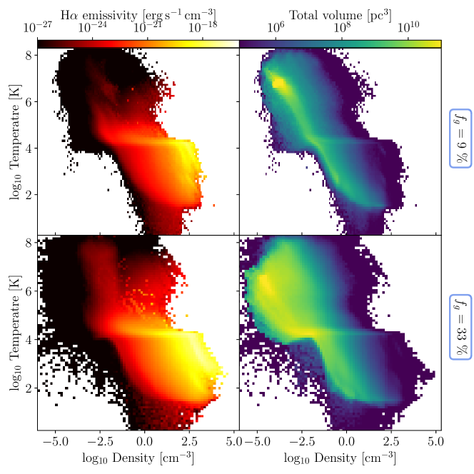
Figure 1: Colour diagrams of gas density-temperature inside the simulated galaxies. Each pixel represents all of the cells with those particular densities and temperatures. Left plots show the H$\alpha$ emissivity weighted-mean of each cell while the right plots are coloured after the volume of cells in each pixel.

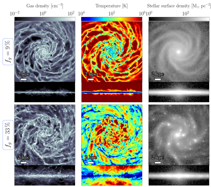
Figure 2: Projection maps of the gas and stellar properties within the simulated galaxies. Each map is projected both face- and edge-on.

2.4 Calculating H$\alpha$ kinematic properties

In this section we detail the calculations of various properties for the gas traced by the H$\alpha$ emission line. We calculate the H$\alpha$ signal directly from the gas in each cell by applying analytical equations of the recombination and collisional rate of the H$\alpha$ emissivity $\epsilon_{\rm H\alpha}$ in each simulation cell. The details of how these equations are derived and calculated is described in Ejdetjärn et al. (2022, see their Appendix C). This approach does not account for absorption and scattering of the H$\alpha$ line on dust. Thus, the H$\alpha$ emission we analyse here is the inherent (or, equivalently, the optically thin/absorption-corrected) emission from the gas.

However, even if we assume our approach is comparable to observations of dust-corrected H$\alpha$ emission, the exact effects of dust-scattering on the H$\alpha$ emission line is complex. In the RHD simulation by Tacchella et al. (2022), the authors performed post-processing of the H$\alpha$ emission and showed that scattering allows 20-40% of their H$\alpha$ emission to escape dust-obscured regions, which increases the H$\alpha$ contribution from dusty HII regions and the relative H$\alpha$ fraction between DIG and HII regions. Furthermore, they show that scattering boosts the H$\alpha$ signal in extraplanar DIG gas. We discuss the potential impact of not including H$\alpha$ dust scattering on our results in Section 4.1 and 4.2.

In order to adequately reproduce the H$\alpha$ signal, the spatial resolution has to be high enough to capture the smallest HII regions. Deng et al. (2023) showed how unresolved HII regions in RHD simulations warm up the surrounding gas and lead to an unrealistic mix of cold and warm gas, resulting in a partially ionised and warm gas ($\sim$8 000 K) which is then overproducing H$\alpha$-bright gas, causing an over-representation of dense HII regions to the total H$\alpha$ signal. In Appendix A, we carry out a post-process analysis of how well resolved, in terms of the Strömgren radius (${\rm R_{SG}}$), photoionised gas is, and investigate the impact of resolution requirements in HII regions. We find that unresolved, hence unrealistic HII regions can be filtered away by requiring ${\rm R_{SG}}$ to be resolved by at least 10 cells (in line with the criterion identified by Deng et al., 2023), which we only enforce in cells with recent star formation, to avoid filtering less H$\alpha$ bright, non-HII regions. Cells which fit this criterion have their $\epsilon_{\rm H\alpha}$ reduced to the mean value of resolved HII regions in our simulations, see Appendix A for details.

After filtering the unresolved HII regions, we achieve a good match for the global H$\alpha$ luminosity ($L_{\rm H\alpha}$, see Table 1) compared to what is predicted from their SFR; by adopting the $L_{\rm H\alpha}$-SFR relation

$$L_{\rm H\alpha}\,[{\rm erg\,s^{-1}}]=1.26\cdot 10^{41}\,\times\,{\rm SFR\,[M_{\odot}\,yr^{-1}]}$$ (2)

from Kennicutt (1998). The predicted values for fg10 and fg30 are $2.5\cdot 10^{41}\ {\rm erg\,s^{-1}cm^{-3}}$ and $5\cdot 10^{42}\ {\rm erg\,s^{-1}cm^{-3}}$, respectively.

In order to illustrate how our H$\alpha$ emissivity calculations perform, and to highlight the gas environment in which the H$\alpha$ signal is the strongest, we show in Figure 1 temperature-density diagrams for each simulation, using one output 200 Myr after the last refinement (see Section 2.4). The left plots are coloured by the H$\alpha$ emissivity and the right plots show the total volume. The left plot can be thought of as a visualisation of the weighting mask that is applied to the data when we calculate H$\alpha$ variables. The strongest H$\alpha$ signal coincides with the temperature- and density-range expected inside HII regions ($T\sim 10\,000$ K, $10{\rm\,m_{H}\,cm^{-3}}\leq\rho\leq 1\,000)\,{\rm m_{H}\,cm^{-3}}$). The diffuse gas ($T\sim 8\,000$ K, $\rho\lesssim 0.1\,{\rm\,m_{H}\,cm^{-3}}$) has notably smaller $\epsilon_{\rm H\alpha}$ but fill a much larger volume and so it still has a significant contribution to the total L_Hα.

The H$\alpha$ properties were calculated by dividing the galaxy into a square grid with 1 x 1 kpc² patches (see e.g. Figure 4). The gas velocity dispersion in H$\alpha$, $\sigma_{\rm H\alpha}$, was calculated as the H$\alpha$ weighted-mean of all simulation cells within each grid patch. We computed mock line profiles of the H$\alpha$ signal within these grids by binning the gas velocity, from $-200$${\,\rm{km\,s^{-1}}}$to $+200$${\,\rm{km\,s^{-1}}}$, and summing up the total H$\alpha$ luminosity in each velocity bin.

The variables presented in Table 1 are time-averaged values for the entire galaxy. We calculated $\sigma_{\rm H\alpha}$ by first calculating $\sigma_{\rm H\alpha}$ within each grid patch and then computing an H$\alpha$ weighted-mean value of these values, as is common to do in observations when the galaxy is resolved. The grid size adopted is 1 kpc, unless otherwise stated, and we briefly explore the impact of grid size on $\sigma_{\rm H\alpha}$ in Section 4.1.

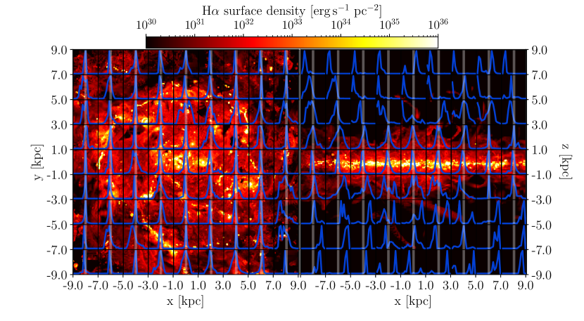
Figure 3: Projection maps, edge- and face-on, of the H$\alpha$ emissivity for the fg30 simulation 200 Myr after the lat refinement step (see Section 2.4). The blue lines in each grid patch is the mock line profile, with velocity range $-200$${\,\rm{km\,s^{-1}}}$ to $+200$${\,\rm{km\,s^{-1}}}$, of the H$\alpha$ emission viewed along the $z$-direction. The line centre (0 km s^-1) is annotated with a weak white line in each grid. The edge-on projection shows clear blue/red-shifted profiles above the gas disc, which is indicative of accelerating outflows.

3 Results

In Figure 2 we show the gas density, gas temperature, and stellar mass density maps for our simulations. A significant difference between the gas fractions is their gas and stellar structure. The lower gas fraction has its cold, dense gas (and therefore also star formation) confined within spiral arms while the higher gas fraction shows more clumpy gas and stellar structure, as found in other theoretical work on gas rich galaxies (e.g. Agertz et al., 2009; Bournaud et al., 2009; Renaud et al., 2021) and observed in high redshift disc galaxies (e.g. Elmegreen et al., 2007; Genzel et al., 2011; Zanella et al., 2019). The maps also reveal that the higher gas fraction galaxy has a more prominent vertical structure, with a high covering fraction of warm gas ($10^{4}~{}{\rm K}<T<10^{5}~{}{\rm K}$) several kiloparsecs above the disc plane, and significant amounts of outflows due to stellar feedback processes (see e.g. Veilleux et al., 2005, for a review). In the next section, we look at the H$\alpha$ bright gas and show, again, how hot, ionised, gas is ejected from the disc. In Section 4.2, we investigate in more detail the gas vertical disc structure and outflows.

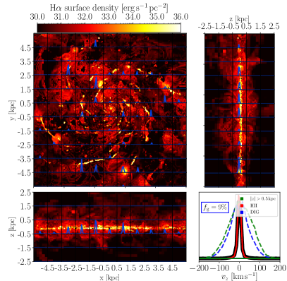
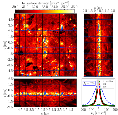
Figure 4: The H$\alpha$ surface density maps, viewed from three angles, of the fg10 (left) and fg30 (right) simulations with mock H$\alpha$ emission line profiles plotted as blue lines on top of them. The line profiles in all projection maps are along the vertical, $z$-direction, integrated along line-of-sight of the grid patches. The total H$\alpha$ profile of the simulations is seen in the lower right (black line), which we also decompose into several components: extra-planar gas, DIG, and HII regions. The dashed lines are profiles normalised to the same max value as the total line. See Section 2.4 for how these mock profiles are calculated.

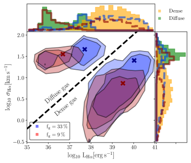
Figure 5: Contours of the relation between the H$\alpha$ velocity dispersion and the H$\alpha$ luminosity. The values were calculated within 1 kpc grids, as described in Section 2.4, and the contours show 90 % and 68 % of the data. The crosses are the L_Hα-weighted mean. The gas is divided into diffuse ($\rho_{\rm g}\leq 0.1\,{\rm cm^{-3}}$) and dense gas ($\rho_{\rm g}\geq 10\,{\rm cm^{-3}}$), which creates two distinct region in this parameter space; highlighted with a dashed line. This indicates a clear separation in H$\alpha$ luminosity and kinematics between (diffuse) DIG and (dense) HII regions. The histograms show the distribution of the diffuse and dense gas, with line-histograms dividing it into the two simulations.

3.1 The H$\alpha$ signal within the galaxy

In this section, we present mock H$\alpha$ line profiles (see Section 2.4 for details) for different spatial locations, inside and outside of the disc, to better understand the origins of profile shapes. In Figure 3 we show the fg30 simulation at 250 Myr projected face- and edge-on ($z$ and $x$ projection) with a 2 x 2 kpc² grid of line-profiles normalised to the same maximum line peak. Both projections show the line profiles in the vertical $z$ direction for all gas within that grid. In the face-on projection (left), there is no clear spatial correlation with the line-width of the profile and the H$\alpha$ bright regions. This is likely due to the grid being too coarse and the projection plots presented next will show a higher spatial resolution. The edge-on projection (right), shows that extraplanar line profiles are much broader than those inside the disc. Furthermore, extraplanar line profiles become increasingly blue- and red-shifted with increasing distance away from the disc, which is due to the accelerating nature of the outflows. This highlights that even if the outflows are not contributing significantly to the total L_Hα (as we argue below), they shape the wings of the observable profile.

The non-normalised line profiles inside of the fg10 and fg30 galaxies can be seen in Figure 4. In each figure, the galaxy is projected along three different axes, but the line profiles shown for the edge-on projections are all along the $z$-axis, i.e. as if observed face-on. This method allows us to quantify the contribution to the face-on H$\alpha$ line profile from gas at different heights and environments within the galaxy. Each figure also contain the total H$\alpha$ line profile of the galaxy as a thick black line, as well as divided into specific components: the extraplanar gas ($|z|>0.5$ kpc), HII regions, and the DIG. The dashed lines are the profiles of the component corresponding to that colour, but normalised to the peak value of the total H$\alpha$ profile. The face-on projections show that regions with the highest levels of $\Sigma_{\rm H\alpha}$ coincide with strong emission lines, as expected. The side-projections reveal that the total line profile is completely dominated by emission from warm gas residing in the midplane of the disc, even for the gas rich galaxy which features vigorous outflows. We further quantify the H$\alpha$ emission and line-width variation with height in Section 4.2 and discuss the strength of the outflows in our simulations.

The line profile decomposition of each galaxy further highlights that gas outside of the disc $|z|>0.5$ kpc provide an insignificant portion of the total H$\alpha$ line profile shape. However, it does have a broader distribution, as can be seen from the normalised (dashed) line, and thus has notably higher $\sigma_{\rm H\alpha}$. Furthermore, in the high gas fraction galaxy, the extraplanar H$\alpha$ profile is stronger, which is expected from a thicker gas disc or more massive gas outflows; although, it is also more narrow due to the disc thickness. We quantify this turbulence increase at higher vertical distance in Section 4.2. Additionally, as the extraplanar gas only contributes a small fraction to the total H$\alpha$ profile, a significant amount of the H$\alpha$ bright, high-velocity gas resides within the disc. This could be explained by the scenario in which gas gets accelerated to high velocities within the disc (e.g. due to supernovae), but has yet to be ejected.

Furthermore, the HII profile follows the total H$\alpha$ profile very closely, meaning that HII regions constitutes the majority of H$\alpha$ emission. Thus, the DIG profile, in both galaxies, is rather weak and contribute only roughly $f_{\rm DIG}\leq 10\%$ of the total L_Hα. We discuss this result in comparison with other observational and numerical work in Section 4.1. However, from the normalised DIG line it is clear that the H$\alpha$ emission line from the DIG is much broader. In the coming section, we separate the gas into DIG and HII regions and quantify the H$\alpha$ line profiles in terms of their L_Hα and velocity dispersion $\sigma_{\rm H\alpha}$, as a proxy for line-width.

3.2 The turbulent nature of H$\alpha$ emitting gas

Observations of the ionised gas with the H$\alpha$ line have shown that disc galaxies are highly turbulent systems (see discussion and references in Section 1). However, it is not clear how gas with different physical states and local environments contribute to the observed broad line profiles. We investigate the multi-phase nature of the H$\alpha$ line by dividing the gas into dense ($\rho_{\rm g}\geq 10\,{\rm cm^{-3}}$) and diffuse gas ($\rho_{\rm g}<0.1\,{\rm cm^{-3}}$), to represent HII regions and the DIG, respectively. In Figure 5, we plot $\sigma_{\rm H\alpha}$ as a function of L_Hα in each grid patch of our two simulations. The plot is divided into two distinct regions based on their density, which is highlighted with a dashed line. Additionally, the figure shows histograms of the L_Hα and $\sigma_{\rm H\alpha}$ distribution for the diffuse and dense gas. The diffuse gas is able to reach velocity dispersions as high as $\sigma_{\rm H\alpha}$ $\lesssim 80$${\,\rm{km\,s^{-1}}}$within individual patches and has a mean value of $\sigma_{\rm H\alpha}$ $\sim 50$${\,\rm{km\,s^{-1}}}$. The denser, more luminous, gas is less turbulent with $\sigma_{\rm H\alpha}\lesssim 40$${\,\rm{km\,s^{-1}}}$and an average value of $\sigma_{\rm H\alpha}\sim 29$${\,\rm{km\,s^{-1}}}$. There is also an evolution with increased gas fraction, with the gas rich galaxy ($f_{\rm g}=33\%$) being more luminous and turbulent than the gas poor case ($f_{\rm g}=9\%$) in both the diffuse and dense ionised gas.

As this figure illustrates, the H$\alpha$ emission originates from, at least, two different gas phases with distinct L_Hα and $\sigma_{\rm H\alpha}$. Separating the gas into these phases is important for interpreting the H$\alpha$ emission line in observational studies. In Section 4.1, we go into more detail about how $\sigma_{\rm H\alpha}$, for the diffuse and dense ionised gas, varies in different density-temperature environments.

4 Discussion

In this Section, we quantify the amount of outflows, using the mass loading factor, and explore the effect of outflows on the total H$\alpha$ line profile. We investigate in more detail the variation in $\sigma_{\rm H\alpha}$ in regions with diverse temperatures and densities.

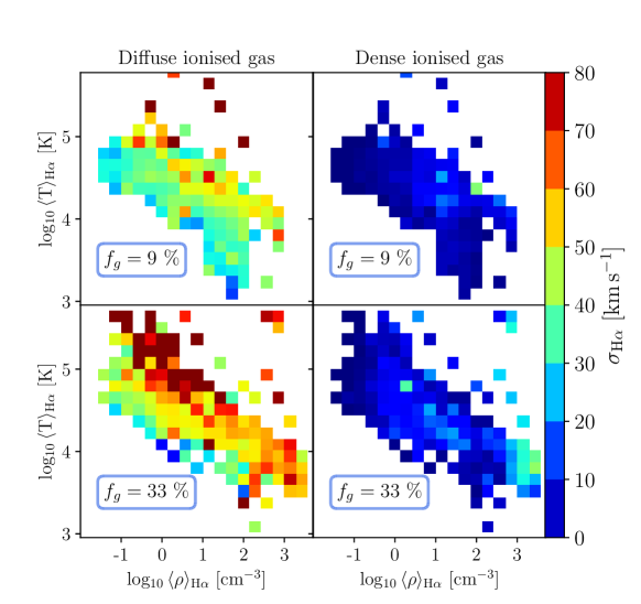
Figure 6: Temperature-density phase diagrams coloured by the H$\alpha$ velocity dispersion in our simulations. The kinematics (but not the temperature or density) were calculated by separating the H$\alpha$ gas into diffuse gas (DIG) and dense gas (HII regions). The temperature $\langle T\rangle_{\rm H\alpha}$ and density $\langle\rho\rangle_{\rm H\alpha}$ presented in this figure are $\epsilon_{\rm H\alpha}$-weighted averages of all the simulation cells within each grid.

4.1 The phase structure of turbulent H$\alpha$ emitting gas

The contribution of H$\alpha$ emission from different gas phases can be understood from the left plots of Figure 1, which indicate that the majority of the H$\alpha$ emission comes from a temperature range around $T\sim 10^{3}-10^{5}$ K, and a wide range of gas densities $\rho\sim 10^{-2}-10^{3}\,{\rm cm^{-3}}$. In Section 3.2 we divided the data into diffuse and dense gas to represent the DIG and HII regions, respectively, and highlighted how the dense ionised gas is less turbulent than the diffuse gas. While the dense HII regions are overall more luminous they also suspend a small volume of the ISM and might thus not represent the overall ionised gas kinematics. Here, we explore how $\sigma_{\rm H\alpha}$varies across these wide temperature and density ranges.

In order to investigate the physical state and turbulence levels of H$\alpha$ emitting gas, we show the gas velocity dispersions, binned in temperature-density phase space, in Figure 6. The temperatures and densities presented in this figure is the $\epsilon_{\rm H\alpha}$-weighted averaged of all the simulations cells in each grid patch. Notably, this means that the (average) gas density is shifted to higher densities compared to the phase diagram of individual simulation cells in Figure 1. We calculate $\sigma_{\rm H\alpha}$ for the diffuse and dense gas separately, but in the same environment; i.e. the temperatures and densities represent mean values of all the gas, but $\sigma_{\rm H\alpha}$ is calculated only for the diffuse or dense gas ($\rho\leq 0.1\,{\rm cm^{-3}}$ and $\rho\geq 10\,{\rm cm^{-3}}$, respectively).

The dense gas exhibits turbulence levels of $\sigma_{\rm H\alpha}\sim 10-20$${\,\rm{km\,s^{-1}}}$, except for in very high density patches in the high gas fraction galaxy, in which it can reach up to $\sigma_{\rm H\alpha}\lesssim 40$${\,\rm{km\,s^{-1}}}$. These high-density patches likely contain H$\alpha$ luminous HII regions, which boost $\sigma_{\rm H\alpha}$, and are confined in small regions. On the other hand, the diffuse gas is ubiquitous throughout (and outside) the disc and is highly turbulent even in the dense environments, i.e. around the HII regions. The diffuse gas in the high gas fraction galaxy has $\sigma_{\rm H\alpha}\sim 50-60$${\,\rm{km\,s^{-1}}}$in most environments and, in the more gas rich galaxy, can reach $\sigma_{\rm H\alpha}\lesssim 80$${\,\rm{km\,s^{-1}}}$in patches with hotter, and more tenuous, gas. Furthermore, the DIG has been observed to be warmer ($T\sim 8\,000$ K) than HII regions ($T\sim 10\,000$ K), which can be seen in this figure. Notably, $\sigma_{\rm H\alpha}$ is slightly larger at the DIG temperatures and lower densities. This highlights the distinct kinematic offset between these two gas phases.

The spatial proximity between the DIG and HII region gas phases, as is seen from observations (e.g. Zurita et al., 2002), is beyond the investigations of this project, but we do note that the strongest H$\alpha$ signals from the diffuse gas are close to the star forming regions. Additionally, the DIG turbulence near the densities of star forming regions ($\rho\sim 100-1000{\rm\,cm^{-3}}$) seem to show slightly higher $\sigma_{\rm H\alpha}$ than the DIG mean (see Figure 6). Furthermore, we check the effects of varying the patch size from which we calculate each parameter. Notably, when using larger patch sizes $\sigma_{\rm H\alpha}$ becomes more skewed towards the lower value associated with HII regions as these dense regions dominate the H$\alpha$ luminosity. If the contribution of L_Hα from DIG regions was higher in our galaxies, $\sigma_{\rm H\alpha}$ might instead increase at lower spatial resolutions.

In Figure 5, there is a clear correlation between L_Hα and $\sigma_{\rm H\alpha}$. These are the most luminous HII regions, which reach upwards of $\sigma_{\rm H\alpha}$ $\approx 40$${\,\rm{km\,s^{-1}}}$, and are regions of recent massive star formation. This connection between SFR and $\sigma_{\rm g}$ is something we explored in detail in Paper I. The driver of global turbulence within galactic disc is still under discussion (see e.g. Krumholz et al., 2018; Ejdetjärn et al., 2022; Ginzburg et al., 2022, and references therein), but it is clear from this figure that the turbulence traced with H$\alpha$ can be strongly tied to these dense HII regions. This implies observations of disc galaxies similar in mass and age to those we present here, with $\sigma_{\rm H\alpha}$ $\gtrsim 40$${\,\rm{km\,s^{-1}}}$require a greater L_Hα contribution from the DIG. Indeed, a similar cut-off has been found for $\sigma_{\rm H\alpha}$ in DIG and HII regions in large-scale surveys (Law et al., 2022). As HII regions are shrouded within molecular clouds, these dense gas phases likely feature similar gas kinematics. Indeed, the offset in $\sigma_{\rm H\alpha}$ between DIG and HII regions in our simulations is reminiscent of the offsets in turbulence levels reported by Girard et al. (2021) for dense molecular gas (as traced by CO) and H$\alpha$ traced ionised gas. We leave the investigation of the relative levels of turbulence between ionised and molecular gas phases to future work (Ejdetjärn et al., in prep).

As discussed in Section 2.4, our approach to calculate H$\alpha$ emission assumes a perfect dust-correction. Accounting for dust absorption in HII regions in our simulations would reduce the amount of H$\alpha$ emission from HII regions and favour the contribution from the DIG, resulting in a boost in the relative DIG/HII region contribution. This, in turn, would shift total $\sigma_{\rm H\alpha}$ towards higher values (i.e. closer to $\sigma_{\rm H\alpha}$ of the DIG). Tacchella et al. (2022) find a 3-5 times higher DIG contribution $f_{\rm DIG}$ than our work, which could possibly be explained by their post-process method of propagating the H$\alpha$ emission through the ISM, which takes into account absorption and scattering of the line. As post-processing would require notably more analysis, we leave dust scattering for future work.

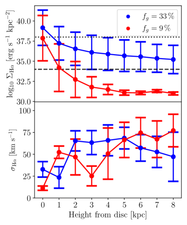
Figure 7: The H$\alpha$ luminosity and velocity dispersion as a function of the height from the disc. The values are time-averaged from several simulation outputs with a 1$\sigma$ errorbar. A sensitivity limit, based on the capabilities of MUSE/JWST within the local/high-redshift universe (comparable to the low/high gas fraction galaxy), is plotted as a dashed/dotted grey line (see the details of how these are determined in Section 4.2).

4.2 Is the H$\alpha$ signal coming from outflows or the disc?

In Section 3.1 we showed that outflows only have a minor contribution to the total H$\alpha$ line profile. In Figure 7 we quantify this by calculating the average L_Hα surface density ($\Sigma_{\rm H\alpha}$) and $\sigma_{\rm H\alpha}$ at different heights. There is a clear, steady decline in the H$\alpha$ brightness for both simulation, which is steeper for the lower gas fraction disc. On the other hand, there is a steady increase in $\sigma_{\rm H\alpha}$ as one moves further from the disc, which can be attributed to fast-speed outflows from the disc with a broad velocity distribution. In particular, fg10 has a sharp increase in $\sigma_{\rm H\alpha}$ just above the disc $\sim$1 kpc, which is due to the disc being thin so outflows dominate the H$\alpha$ gas close to the disc (compared to fg30 with a more extended gas disc height). Due to the low average H$\alpha$ surface brightness above the disc, the H$\alpha$ gas in fg10 would not be observable beyond 1.5-2 kpc if observed with MUSE (assuming an integration time of a couple of hours and galaxy-wide homogeneous slabs with 1 kpc height). This applies to a object in the local universe, where a gas fraction of $\sim 10\%$ is appropriate.

However, the extraplanar H$\alpha$ luminosity is dominated by few bright patches (from bright filaments), and such bright individual 1 kpc² patches would be detectable to larger heights when present. The higher gas fraction galaxy is much brighter but is assumed to be further away, as it is modelled to represent the same type of galaxy at a redshift of $z\sim 1-2$. Using JWST NIRSPEC/IFU for $\sim$10 hours would allow the high-redshift galaxy to be observable in slabs to heights 2-3 kpc, but again the brightest individual kpc² sized cells would be detectable to larger heights. Hence, the predictions of our models are in principle testable with deep VLT or JWST observations.

The mass loading factor $\eta=\dot{M}/{\rm SFR}$, which quantifies the amount of gas mass flowing out from the galaxy relative to its star formation rate, is presented in Figure 8 as a function of height from the disc. Our high gas fraction simulation has $\eta\sim 0.5-1$ at a height of a few kpc. Observations of local galaxies with similar stellar masses, $M_{*}\sim 10^{10}$, are in agreement with ours but there is a large spread $\eta\sim 0.01-10$ (Chisholm et al., 2017, 2018; Schroetter et al., 2019). On the other hand, our low gas fraction galaxy, equivalent to a local disc, has $\eta\sim 0.1-0.2$ and is thus on the lower limit. Importantly, our galaxies have outflows that are within the expectations from observations and still the amount of H$\alpha$ emission in the extraplanar gas is low. This confirms that our simulations have realistic outflows and that the weak extraplanar H$\alpha$ emission is indeed a property of these types of disc galaxies.

We note that our simulations are not cosmological, meaning that any gas above the disc originated either from disc outflows or from the circumgalactic medium that was initiated with the galaxy. It is possible that inflows or minor mergers could contribute to strip more gas from the disc to these heights, to increase the disc thickness, or allow for more shocked, warm, gas. More massive or gas-rich disc galaxies with more bursty SFRs could possibly have more volatile outflows, resulting in higher $\eta$ and H$\alpha$ above the disc. This could then strengthen the H$\alpha$ signal at these heights. As we are not using post-processing to trace emission line propagation, the H$\alpha$ line is unaffected by dust absorption and scattering. Extraplanar H$\alpha$ emission from dust scattering has been found to contribute $\sim 5-20\%$ (Wood & Reynolds, 1999; Barnes et al., 2015) of the total luminosity. This was also numerically shown by (Tacchella et al., 2022), who found that dust scattering contributed 10-30% of their H$\alpha$ emission above the disc. Furthermore, our models do not include magnetic fields or black hole feedback which could help drive outflows and increase the H$\alpha$ emission and turbulence outside of the disc (and in the DIG).

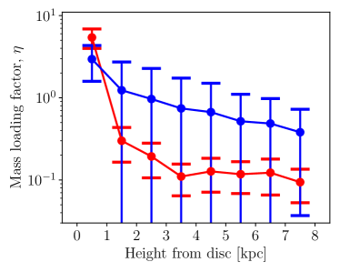
Figure 8: The mass loading factor as a function of the height from the disc. The values are averaged from several simulation outputs with a 1$\sigma$ errorbar.

5 Conclusions

The H$\alpha$ emission line is a versatile observational tool for deriving various properties in both low- and high-redshift galaxies. However, H$\alpha$ is emitted by both dense and diffuse gas, which contribute differently to the H$\alpha$ emission line profile. Furthermore, H$\alpha$ bright diffuse ionised gas is ubiquitous inside and around the galactic disc. Untangling the various contributions to the H$\alpha$ line is important for interpreting the underlying, complex physical processes.

In this paper, we present radiation hydrodynamic simulations of isolated disc galaxies in order to evaluate the strength and kinematics of H$\alpha$ emitting gas in outflows, diffuse disc gas region, and dense gas regions. We model Milky Way-like galaxies, in terms of mass and size, with different gas fractions ($f_{\rm g}=9\%$ and 33%) as a proxy of the galaxy at different epochs of its evolution. We carry out mock observation of the H$\alpha$ emission line, which, after careful numerical treatment of unresolved HII regions (Appendix A), match empirical L_Hα-SFR relations (Kennicutt, 1998).

The key findings in this work are summarised below:

1. We highlight a distinct difference in the H$\alpha$ luminosity and kinematic signature between the diffuse and dense gas emitting strongly in H$\alpha$, as is also found between observations of DIG and dense HII region gas (see e.g. Law et al., 2022, and references therein). In the gas rich galaxy ($f_{\rm g}=33\%$), the dense gas reaches at most $\sigma_{\rm H\alpha}$ $\lesssim 40$${\,\rm{km\,s^{-1}}}$, with a mean value of 29${\,\rm{km\,s^{-1}}}$, while the diffuse gas reaches $\sigma_{\rm H\alpha}\lesssim 80\,{\rm km\,s^{-1}}$, with a mean value of 54${\,\rm{km\,s^{-1}}}$.

2. The H$\alpha$ emission line is broader in the younger, i.e. higher gas fraction, galaxy. The low gas fraction galaxy has an H$\alpha$ emission line (ionised gas) roughly half as broad (turbulent) when looking at the total H$\alpha$ emission. This is also true for H$\alpha$ emission from dense, HII regions. However, the H$\alpha$ emission in the DIG has a more shallow evolution.

3. The contribution of the diffuse gas to L_Hα is approximated to be $\lesssim 10\,\%$ for H$\alpha$ emitting gas below $\rho_{\rm H}\lesssim 0.1\,{\rm cm^{-3}}$. This matches with the lower-limits found by observations of the DIG (see the discussion in Section 1). However, several studies suggests the DIG can constitute the majority of L_Hαand numerical work with similar setup to ours, by Tacchella et al. (2022), agrees with this high DIG fraction. The major difference with our setup is that we do not perform post-processing to trace the H$\alpha$ emission line. Our study encourages further work into post-processing of H$\alpha$ emission line propagation in RHD simulations, to capture the impact of dust scattering and absorption on the observed H$\alpha$ line profile.

4. Gas outside of the galactic disc contribute very little to the total H$\alpha$ signal, despite that the mass outflow in our high gas-fraction galaxy match with observed values of galaxies with similar stellar mass. Thus, the overall galaxy disc dynamics could be well-constrained with observations of H$\alpha$, taking into consideration any kinematic offset between the DIG and HII regions (see points above).

5. The $\sigma_{\rm H\alpha}$ of gas that exists several kpc above the disc is much more turbulent compared to the mid-plane, increasing by a factor of 2-4 depending on the simulation. However, the luminosity at these heights corresponds to only a few percent of the total L_Hα, which has an H$\alpha$ surface density below the sensitivity limit of MUSE in local galaxies and JWST at redshift $\sim 1.5$ (see Section 4.2). This suggests that the H$\alpha$ emission can be readily observed a few kpc above the disc and the predictions of our simulations on the H$\alpha$ vertical structure can be tested.

Data Availability

The data underlying this article will be shared on reasonable request to the corresponding author.

Appendix A The impact of unresolved HII regions on H$\alpha$ parameters

Deng et al. (2023) showed that to properly resolve the HII regions in numerical simulations, the Strömgren radius needs to be resolved by 10-100 simulation cells. Not resolving the HII regions causes these cells to be heated up by the ionising radiation from the bright stars within, which results in an unrealistic gas mix of partially-ionised, warm ($T\sim 8\,000$ K), dense ($\rho\geq 100\,{\rm cm^{-3}}$) gas. These artificial conditions are prime for H$\alpha$ emission and can contaminate analysis of H$\alpha$ quantities. Here we evaluate the impact of unresolved HII regions on the H$\alpha$ emission and kinematics computed in this paper.

The size of an idealised HII region can approximated by the Strömgren radius. The equation describes the size of a spherical ionised bubble formed as one or more very young and luminous stars ionise the surrounding gas, and can be written as

$$R_{\rm SG}=\bigg{(}{\frac{3Q_{0}}{4\pi n_{\rm H}^{2}\alpha_{\rm B}}}\bigg{)}^{1/3}.$$ (3)

Here, $Q_{0}$ is the rate of ionising photons emitted by the stars, $n_{\rm H}$ is the hydrogen density, and $\alpha_{\rm B}$ is the effective hydrogen recombination rate, which can be described as a function of gas temperature

$$\alpha_{\rm B}(T)=2.753\cdot 10^{-14}\,\bigg{(}\frac{315614}{T}\bigg{)}^{1.5}\Bigg{(}1+\bigg{(}\frac{315614}{T}\bigg{)}^{0.407}\Bigg{)}^{-2.42}.$$ (4)

This expression is a fit made by Hui & Gnedin (1997), using observational data from Ferland et al. (1992).

We implement a criteria for the number of resolved Strömgren radii ($R_{\rm SG}/\Delta x$) in our simulations by reducing the H$\alpha$ emissivity to the mean value of resolved HII regions in our galaxies ($\epsilon_{\rm H\alpha}=2\cdot 10^{-20}{\rm erg\,s^{-1}\,cm^{-3}}$ for fg30 and $\epsilon_{\rm H\alpha}=7\cdot 10^{-21}{\rm erg\,s^{-1}\,cm^{-3}}$ for fg10) for the regions unresolved by a certain amount of cells. Figure 9 shows L_Hα and $\sigma_{\rm H\alpha}$ as a function of how many cells $R_{\rm SG}$ is resolved. As can be seen, there is a strong decrease in the H$\alpha$ luminosity at 1-10 cells resolved, as most of the highly luminous, and unresolved, regions are filtered away. When $R_{\rm SG}/\Delta x\approx 10$ unresolved cells are filtered, the decrease in luminosity is much more shallow, indicating that the most problematic cells have been corrected. The expected luminosity from the L_Hα-SFR relation (Kennicutt, 1998) for these SFRs is around $2.5\cdot 10^{41}{\rm erg\,s^{-1}\,cm^{-3}}$ and $5\cdot 10^{42}{\rm erg\,s^{-1}\,cm^{-3}}$ for the low- and high-gas fraction simulations, respectively. All of this indicates that by filtering cells that do not resolve the Strömgren sphere with at least 10 cells, we correct for most of the unresolved HII regions and achieve a much better match with L_Hα predicted.

Furthermore, the lower plot in this figure suggests that the H$\alpha$ velocity dispersion for the entire galaxy remains largely unaffected by this filtering process. However, this $\sigma_{\rm H\alpha}$ is integrated over the entire galaxy (comparable to observations of unresolved galaxies), rather than computing $\sigma_{\rm H\alpha}$ in each grid patch and then calculating a mean value from that, which is the common approach for resolved galaxy observations. Therefore, it is not directly comparable to $\sigma_{\rm H\alpha}$ we compute in the main body of the text, but, as discussed in Section 4.1, $\sigma_{\rm H\alpha}$ remains largely unaffected by altering the grid patch size.

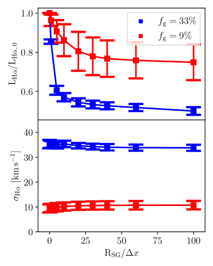
Figure 9: The H$\alpha$ luminosity and velocity dispersion above different criteria for resolving the Strömgren sphere $R_{\rm SG}$ with cells of size $\Delta x$. ${\rm L_{H\alpha,\,0}}$ here is the un-filtered luminosity of each simulations, which is $5.5\cdot 10^{41}\,{\rm erg\,s^{-1}}$ and $8.5\cdot 10^{42}\,{\rm erg\,s^{-1}}$ for fg10 and fg30, respectively.

References

- Agertz & Kravtsov (2015) Agertz O., Kravtsov A. V., 2015, ApJ, 804, 18
- Agertz & Kravtsov (2016) Agertz O., Kravtsov A. V., 2016, ApJ, 824, 79
- Agertz et al. (2009) Agertz O., Teyssier R., Moore B., 2009, MNRAS, 397, L64
- Agertz et al. (2013) Agertz O., Kravtsov A. V., Leitner S. N., Gnedin N. Y., 2013, ApJ, 770, 25
- Agertz et al. (2020) Agertz O., et al., 2020, MNRAS, 491, 1656
- Agertz et al. (2021) Agertz O., et al., 2021, MNRAS, 503, 5826
- Alcorn et al. (2018) Alcorn L. Y., et al., 2018, ApJ, 858, 47
- Armillotta et al. (2018) Armillotta L., Krumholz M. R., Fujimoto Y., 2018, MNRAS, 481, 5000
- Armus et al. (1987) Armus L., Heckman T., Miley G., 1987, AJ, 94, 831
- Asplund et al. (2009) Asplund M., Grevesse N., Sauval A. J., Scott P., 2009, ARA&A, 47, 481
- Barnes et al. (2015) Barnes J. E., Wood K., Hill A. S., Haffner L. M., 2015, MNRAS, 447, 559
- Belfiore et al. (2022) Belfiore F., et al., 2022, A&A, 659, A26
- Bigiel et al. (2008) Bigiel F., Leroy A., Walter F., Brinks E., de Blok W. J. G., Madore B., Thornley M. D., 2008, AJ, 136, 2846
- Bik et al. (2022) Bik A., Östlin G., Hayes M., Melinder J., Menacho V., 2022, A&A, 666, A161
- Binette et al. (2009) Binette L., Flores-Fajardo N., Raga A. C., Drissen L., Morisset C., 2009, ApJ, 695, 552
- Blanc et al. (2009) Blanc G. A., Heiderman A., Gebhardt K., Evans Neal J. I., Adams J., 2009, ApJ, 704, 842
- Bournaud et al. (2009) Bournaud F., Elmegreen B. G., Martig M., 2009, ApJ, 707, L1
- Bruzual & Charlot (2003) Bruzual G., Charlot S., 2003, MNRAS, 344, 1000
- Carpineti et al. (2015) Carpineti A., Kaviraj S., Hyde A. K., Clements D. L., Schawinski K., Darg D., Lintott C. J., 2015, A&A, 577, A119
- Chabrier (2003) Chabrier G., 2003, Publications of the Astronomical Society of the Pacific, 115, 763
- Chisholm et al. (2017) Chisholm J., Tremonti C. A., Leitherer C., Chen Y., 2017, MNRAS, 469, 4831
- Chisholm et al. (2018) Chisholm J., Tremonti C., Leitherer C., 2018, MNRAS, 481, 1690
- Collins & Rand (2001) Collins J. A., Rand R. J., 2001, The Astrophysical Journal, 551, 57
- Cresci et al. (2009) Cresci G., et al., 2009, ApJ, 697, 115
- Della Bruna et al. (2020) Della Bruna L., et al., 2020, A&A, 635, A134
- Della Bruna et al. (2022) Della Bruna L., et al., 2022, A&A, 660, A77
- Deng et al. (2023) Deng Y., Li H., Kannan R., Smith A., Vogelsberger M., Bryan G. L., 2023, MNRAS,
- Di Teodoro & Fraternali (2015) Di Teodoro E. M., Fraternali F., 2015, MNRAS, 451, 3021
- Dib et al. (2006) Dib S., Bell E., Burkert A., 2006, ApJ, 638, 797
- Dirks et al. (2023) Dirks L., Dettmar R. J., Bomans D. J., Kamphuis P., Schilling U., 2023, A&A, 678, A84
- Ejdetjärn et al. (2022) Ejdetjärn T., Agertz O., Östlin G., Renaud F., Romeo A. B., 2022, MNRAS, 514, 480
- Elmegreen & Scalo (2004) Elmegreen B. G., Scalo J., 2004, Annual Review of Astronomy and Astrophysics, 42, 211
- Elmegreen et al. (2007) Elmegreen D. M., Elmegreen B. G., Ravindranath S., Coe D. A., 2007, ApJ, 658, 763
- Epinat et al. (2010) Epinat B., Amram P., Balkowski C., Marcelin M., 2010, MNRAS, 401, 2113
- Faucher-Giguère et al. (2009) Faucher-Giguère C.-A., Lidz A., Zaldarriaga M., Hernquist L., 2009, ApJ, 703, 1416
- Faucher-Giguère et al. (2011) Faucher-Giguère C.-A., Kereš D., Ma C.-P., 2011, MNRAS, 417, 2982
- Federrath (2018) Federrath C., 2018, Physics Today, 71, 38
- Ferguson et al. (1996) Ferguson A. M. N., Wyse R. F. G., Gallagher J. S., Hunter D. A., 1996, in Kunth D., Guiderdoni B., Heydari-Malayeri M., Thuan T. X., eds, Vol. 11, The Interplay Between Massive Star Formation, the ISM and Galaxy Evolution. p. 513 (arXiv:astro-ph/9602069), doi:10.48550/arXiv.astro-ph/9602069
- Ferland et al. (1992) Ferland G. J., Peterson B. M., Horne K., Welsh W. F., Nahar S. N., 1992, ApJ, 387, 95
- Ferland et al. (1998) Ferland G. J., Korista K. T., Verner D. A., Ferguson J. W., Kingdon J. B., Verner E. M., 1998, PASP, 110, 761
- Forbes et al. (2023) Forbes J. C., et al., 2023, ApJ, 948, 107
- Genzel et al. (2011) Genzel R., et al., 2011, ApJ, 733, 101
- Ginzburg et al. (2022) Ginzburg O., Dekel A., Mandelker N., Krumholz M. R., 2022, arXiv e-prints, p. arXiv:2202.12331
- Girard et al. (2021) Girard M., et al., 2021, ApJ, 909, 12
- Glazebrook (2013) Glazebrook K., 2013, Publications of the Astronomical Society of Australia, 30, e056
- Gnedin et al. (2009) Gnedin N. Y., Tassis K., Kravtsov A. V., 2009, ApJ, 697, 55
- Green et al. (2014) Green A. W., et al., 2014, MNRAS, 437, 1070
- Grisdale et al. (2018) Grisdale K., Agertz O., Renaud F., Romeo A. B., 2018, MNRAS,
- Grisdale et al. (2019) Grisdale K., Agertz O., Renaud F., Romeo A. B., Devriendt J., Slyz A., 2019, arXiv e-prints,
- Guillet & Teyssier (2011) Guillet T., Teyssier R., 2011, Journal of Computational Physics, 230, 4756
- Haffner et al. (2009) Haffner L. M., et al., 2009, Reviews of Modern Physics, 81, 969
- Harris et al. (2020) Harris C. R., et al., 2020, Nature, 585, 357–362
- Hayward & Hopkins (2017) Hayward C. C., Hopkins P. F., 2017, MNRAS, 465, 1682
- Heckman & Best (2014) Heckman T. M., Best P. N., 2014, ARA&A, 52, 589
- Herenz et al. (2016) Herenz E. C., et al., 2016, A&A, 587, A78
- Hernquist (1990) Hernquist L., 1990, ApJ, 356, 359
- Ho et al. (2016) Ho I. T., et al., 2016, MNRAS, 457, 1257
- Hoopes et al. (1996) Hoopes C. G., Walterbos R. A. M., Greenwalt B. E., 1996, AJ, 112, 1429
- Hui & Gnedin (1997) Hui L., Gnedin N. Y., 1997, MNRAS, 292, 27
- Hunter (2007) Hunter J. D., 2007, Computing in Science & Engineering, 9, 90
- Katz et al. (2019) Katz H., et al., 2019, MNRAS, 487, 5902
- Kennicutt (1998) Kennicutt Jr. R. C., 1998, ARA&A, 36, 189
- Kim & Ostriker (2015) Kim C.-G., Ostriker E. C., 2015, ApJ, 802, 99
- Kim et al. (2014) Kim J.-h., et al., 2014, ApJS, 210, 14
- Kim et al. (2016) Kim J.-h., et al., 2016, ApJ, 833, 202
- Kohandel et al. (2023) Kohandel M., Pallottini A., Ferrara A., Zanella A., Rizzo F., Carniani S., 2023, arXiv e-prints, p. arXiv:2311.05832
- Kreckel et al. (2016) Kreckel K., Blanc G. A., Schinnerer E., Groves B., Adamo A., Hughes A., Meidt S., 2016, ApJ, 827, 103
- Krumholz & Tan (2007) Krumholz M. R., Tan J. C., 2007, ApJ, 654, 304
- Krumholz et al. (2018) Krumholz M. R., Burkhart B., Forbes J. C., Crocker R. M., 2018, MNRAS, 477, 2716
- Larson (1981) Larson R. B., 1981, MNRAS, 194, 809
- Law et al. (2009) Law D. R., Steidel C. C., Erb D. K., Larkin J. E., Pettini M., Shapley A. E., Wright S. A., 2009, ApJ, 697, 2057
- Law et al. (2022) Law D. R., et al., 2022, ApJ, 928, 58
- Lelli et al. (2023) Lelli F., et al., 2023, A&A, 672, A106
- Levermore (1984) Levermore C. D., 1984, J. Quant. Spectrosc. Radiative Transfer, 31, 149
- Levy et al. (2018) Levy R. C., et al., 2018, ApJ, 860, 92
- Mac Low & Klessen (2004) Mac Low M.-M., Klessen R. S., 2004, Reviews of Modern Physics, 76, 125
- McKee & Ostriker (1977) McKee C. F., Ostriker J. P., 1977, ApJ, 218, 148
- McKee & Ostriker (2007) McKee C. F., Ostriker E. C., 2007, ARA&A, 45, 565
- Micheva et al. (2022) Micheva G., et al., 2022, A&A, 668, A74
- Minter & Spangler (1997) Minter A. H., Spangler S. R., 1997, The Astrophysical Journal, 485, 182
- Moiseev et al. (2015) Moiseev A. V., Tikhonov A. V., Klypin A., 2015, MNRAS, 449, 3568
- Navarro et al. (1996) Navarro J. F., Frenk C. S., White S. D. M., 1996, ApJ, 462, 563
- Nguyen-Luong et al. (2016) Nguyen-Luong Q., et al., 2016, ApJ, 833, 23
- Nickerson et al. (2019) Nickerson S., Teyssier R., Rosdahl J., 2019, MNRAS, 484, 1238
- Oey et al. (2007) Oey M. S., et al., 2007, ApJ, 661, 801
- Orr et al. (2020) Orr M. E., et al., 2020, MNRAS, 496, 1620
- Osterbrock & Ferland (2006) Osterbrock D. E., Ferland G. J., 2006, Astrophysics of gaseous nebulae and active galactic nuclei
- Östlin et al. (2001) Östlin G., Amram P., Bergvall N., Masegosa J., Boulesteix J., Márquez I., 2001, A&A, 374, 800
- Rand (1996) Rand R. J., 1996, ApJ, 462, 712
- Rathjen et al. (2023) Rathjen T.-E., Naab T., Walch S., Seifried D., Girichidis P., Wünsch R., 2023, MNRAS, 522, 1843
- Renaud et al. (2012) Renaud F., Kraljic K., Bournaud F., 2012, ApJ, 760, L16
- Renaud et al. (2014) Renaud F., Bournaud F., Kraljic K., Duc P. A., 2014, MNRAS, 442, L33
- Renaud et al. (2021) Renaud F., Romeo A. B., Agertz O., 2021, MNRAS, 508, 352
- Rizzo et al. (2022) Rizzo F., Kohandel M., Pallottini A., Zanella A., Ferrara A., Vallini L., Toft S., 2022, A&A, 667, A5
- Rosdahl & Teyssier (2015) Rosdahl J., Teyssier R., 2015, MNRAS, 449, 4380
- Rosdahl et al. (2013) Rosdahl J., Blaizot J., Aubert D., Stranex T., Teyssier R., 2013, MNRAS, 436, 2188
- Rosen & Bregman (1995) Rosen A., Bregman J. N., 1995, ApJ, 440, 634
- Rossa et al. (2004) Rossa J., Dettmar R.-J., Walterbos R. A. M., Norman C. A., 2004, AJ, 128, 674
- Sanders et al. (1988) Sanders D. B., Soifer B. T., Elias J. H., Madore B. F., Matthews K., Neugebauer G., Scoville N. Z., 1988, ApJ, 325, 74
- Schmidt (1959) Schmidt M., 1959, ApJ, 129, 243
- Schroetter et al. (2019) Schroetter I., et al., 2019, MNRAS, 490, 4368
- Scoville et al. (2015) Scoville N., et al., 2015, ApJ, 800, 70
- Scoville et al. (2017) Scoville N., et al., 2017, ApJ, 836, 66
- Somerville & Davé (2015) Somerville R. S., Davé R., 2015, ARA&A, 53, 51
- Tacchella et al. (2022) Tacchella S., et al., 2022, MNRAS, 513, 2904
- Tamburro et al. (2009) Tamburro D., Rix H.-W., Leroy A. K., Mac Low M.-M., Walter F., Kennicutt R. C., Brinks E., de Blok W. J. G., 2009, AJ, 137, 4424
- Teyssier (2002) Teyssier R., 2002, A&A, 385, 337
- Toro et al. (1994) Toro E. F., Spruce M., Speares W., 1994, Shock Waves, 4, 25
- Turk et al. (2011) Turk M. J., Smith B. D., Oishi J. S., Skory S., Skillman S. W., Abel T., Norman M. L., 2011, ApJS, 192, 9
- Übler et al. (2019) Übler H., et al., 2019, ApJ, 880, 48
- Vandenbroucke & Wood (2019) Vandenbroucke B., Wood K., 2019, MNRAS, 488, 1977
- Vandenbroucke et al. (2018) Vandenbroucke B., Wood K., Girichidis P., Hill A. S., Peters T., 2018, MNRAS, 476, 4032
- Varidel et al. (2016) Varidel M., Pracy M., Croom S., Owers M. S., Sadler E., 2016, Publications of the Astronomical Society of Australia, 33, e006
- Veilleux et al. (2005) Veilleux S., Cecil G., Bland-Hawthorn J., 2005, ARA&A, 43, 769
- Veilleux et al. (2009) Veilleux S., et al., 2009, ApJS, 182, 628
- Weilbacher et al. (2018) Weilbacher P. M., et al., 2018, A&A, 611, A95
- Wisnioski et al. (2011) Wisnioski E., et al., 2011, MNRAS, 417, 2601
- Wood & Reynolds (1999) Wood K., Reynolds R. J., 1999, ApJ, 525, 799
- Yang & Krumholz (2012) Yang C.-C., Krumholz M., 2012, ApJ, 758, 48
- Zanella et al. (2019) Zanella A., et al., 2019, MNRAS, 489, 2792
- Zurita et al. (2002) Zurita A., Beckman J. E., Rozas M., Ryder S., 2002, A&A, 386, 801
- den Brok et al. (2020) den Brok M., et al., 2020, MNRAS, 491, 4089
- van Dokkum et al. (2013) van Dokkum P. G., et al., 2013, ApJ, 771, L35