Online Test-Time Adaptation of Spatial-Temporal Traffic Flow Forecasting

Abstract

Accurate spatial-temporal traffic flow forecasting is crucial in aiding traffic managers in implementing control measures and assisting drivers in selecting optimal travel routes. Traditional deep-learning based methods for traffic flow forecasting typically rely on historical data to train their models, which are then used to make predictions on future data. However, the performance of the trained model usually degrades due to the temporal drift between the historical and future data. To make the model trained on historical data better adapt to future data in a fully online manner, this paper conducts the first study of the online test-time adaptation techniques for spatial-temporal traffic flow forecasting problems. To this end, we propose an Adaptive Double Correction by Series Decomposition (ADCSD) method, which first decomposes the output of the trained model into seasonal and trend-cyclical parts and then corrects them by two separate modules during the testing phase using the latest observed data entry by entry. In the proposed ADCSD method, instead of fine-tuning the whole trained model during the testing phase, a lite network is attached after the trained model, and only the lite network is fine-tuned in the testing process each time a data entry is observed. Moreover, to satisfy that different time series variables may have different levels of temporal drift, two adaptive vectors are adopted to provide different weights for different time series variables. Extensive experiments on four real-world traffic flow forecasting datasets demonstrate the effectiveness of the proposed ADCSD method. The code is available at https://github.com/Pengxin-Guo/ADCSD.

I Introduction

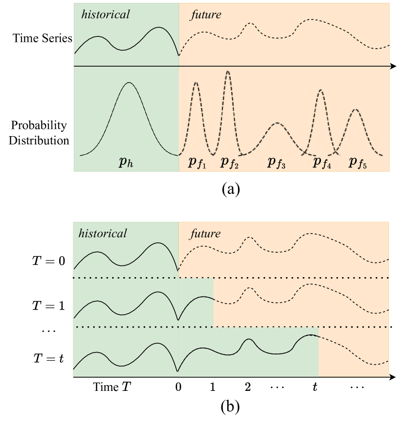
Figure 1: (a). The temporal drift problem in non-stationary time series. The raw time series data is multivariate in reality. As our focus is on the distribution of the future data rather than the historical data, we assume that the historical data follows one distribution $p_{h}$, although it is possible for it to follow multiple distributions. For the future data, the distribution will changes over time, i.e., $p_{f_{1}}\neq p_{f_{2}}\neq p_{f_{3}}\neq p_{f_{3}}\neq p_{f_{4}}\neq p_{f_{5}}\neq p_{h}.$ (b). Data identity change. With the time goes by, the future data will become historical data.

Spatial-temporal traffic flow forecasting is a key component of intelligent transportation systems (ITS) and has received significant attentions in recent years [1, 2, 3, 4, 5, 6]. Most deep learning-based traffic flow forecasting methods train models on historical data and make predictions on future data without modifying the trained model [7, 8, 9, 10]. However, the performance of those models is usually unsatisfactory due to the non-stationarity of time series data, i.e., temporal drift between the historical and future data [11, 12] (see Figure 1(a)). This temporal drift could stem from changes in upstream processes, sensors, materials, natural drift, or variable relation shifts, etc. To solve the temporal drift problem, some works [12, 13] aim to learn distribution-aware knowledge to aid in model training by assuming that future data follow a different distribution from the historical data. However, it is challenging to assume the availability of the distribution for future data, as it often changes over time, as illustrated in Figure 1(a). Moreover, those methods do not take into consideration the relativity of data identity. That is, the definition of history and future in time series data is relative, as the historical data accrues over time, as shown in Figure 1(b).

To handle those problems faced in spatial-temporal traffic flow forecasting, we study the Online Test-Time Adaptation (OTTA) techniques [14, 15, 16]. OTTA techniques are widely adopted in computer vision (CV) community to address the distribution shift issue by continuously updating and refining the model during the testing phase, based on the feedback and new data encountered during deployment [17, 18, 19, 20]. This adaptive process allows the model to learn and adjust its predictions in real-time, improving its performance and generalization to new data. Though OTTA has been studied in the CV community, to the best of our knowledge, there is no work for spatial-temporal traffic flow forecasting and in this paper, we will give the first try on it. There are some OTTA methods [17, 18, 19, 20] proposed to solve CV problems, but directly applying them to solve spatial-temporal traffic flow forecasting problem may not give satisfactory performance as they do not consider the complex spatial and temporal correlations present in spatial-temporal data and the distribution shift problem that occurs over time. Furthermore, as mentioned above, the relativity of data identity property (see Figure 1(b)) in time series data is also a crucial distinction from CV problems, which is defined as follows: at time $t+1$, we can observe the true label of data $\mathbf{x}_{t}$. Thus, after we make predictions on data $\mathbf{x}_{t}$ at time $t$, we can utilize the ground-truth label information $\mathbf{y}_{t}$ at time $t+1$ to update the model, which is not taken into consideration in existing OTTA methods.

To apply OTTA techniques to the spatial-temporal traffic flow forecasting problem, there are several challenges. Firstly, simply fine-tuning the trained model on spatial-temporal data streams may impair the performance of the model, as we only have access to one data point at a time. Secondly, spatial-temporal data often suffer from the distribution shift problem [12, 13], meaning that the data distribution tends to change over time (see Figure 1(a)). Thirdly, spatial-temporal data is typically composed of multiple time series variables with different levels of temporal drift and the relationship between different time series variables is complicated [8, 21], making the problem more complex. Therefore, applying OTTA to spatial-temporal data is a non-trivial problem and requires further studies.

To address above problems, we propose the Adaptive Double Correction by Series Decomposition (ADCSD) method, which first decomposes the output of the trained model into seasonal and trend-cyclical parts and then corrects them by two separate modules. Specifically, to solve the first issue discussed in the previous paragraph, inspired by Fast Weight Layers (FWLs) [22], instead of fine-tuning the whole trained model, we attach a lite network after the trained model and fine-tune the lite network. To tackle the second issue, we first take the idea of decomposition [23], a standard time series analysis method, to decompose the series into seasonal and trend-cyclical parts and then adopt two modules to correct them, respectively. Benefiting from that such decomposition can ravel out the entangled temporal patterns and highlight the inherent properties of time series [24], we can easily correct the temporal drift between the future data and historical data. Then we add the original output of the trained model with the corrected seasonal and trend-cyclical parts to obtain the final corrected output to conquer the temporal drift problem. For the third issue mentioned above, we design two adaptive vectors to implicitly involve the interaction of spatial information between time series variables and balance the weight between the original output and corrected seasonal and trend-cyclical parts to fit different time series variables with different levels of temporal drift. In summary, our contributions are as follows.

• To the best of our knowledge, we are the first to apply OTTA to spatial-temporal traffic flow forecasting problems.

• To deal with the temporal drift problem, we propose the ADCSD method, which can be used by various spatial-temporal traffic flow deep models in a plug-and-play manner to improve their performance.

• Extensive experiments on both graph-based and grid-based traffic flow forecasting datasets demonstrate the effectiveness of the proposed ADCSD method.

II Related Work

II-A Spatial-Temporal Traffic Flow Forecasting

Spatial-temporal traffic flow forecasting, which combines both spatial and temporal information to predict how the traffic flow will change over time and space, has attracted much attention in recent years [25, 26, 27, 6, 28, 29]. To perform reliable and accurate traffic flow forecasting, many models have been proposed [7, 8, 30, 10]. For example, Attention based Spatial-Temporal Graph Convolutional Networks (ASTGCN) [7] that consists of three independent components to respectively model three temporal properties of traffic flows, i.e., recent, daily-periodic and weekly-periodic dependencies, Adaptive Graph Convolutional Recurrent Network (AGCRN) [8] that can capture fine-grained spatial and temporal correlations in traffic series automatically based on two module (i.e., Node Adaptive Parameter Learning module and Data Adaptive Graph Generation module) and recurrent networks, Attention based Spatial-Temporal Graph Neural Network (ASTGNN) [30] that consists of a novel self-attention mechanism to capture the temporal dynamics of traffic data and a dynamic graph convolution module to capture the spatial correlations in a dynamic manner, Propagation Delay-aware Dynamic Long-range Transformer (PDFormer) [10] that consists of a spatial self-attention module to capture the dynamic spatial dependencies and two graph masking matrices to highlight spatial dependencies from short- and long-range views, etc. However, all of those methods train models on the historical data and make predictions on the future data without modifying the trained model. Thus, the trained model usually cannot give satisfactory performance due to the non-stationary of time series data, i.e., temporal drift between the historical and future data [11, 12]. Some works attempt to solve this problem [12, 31, 32, 33, 13, 34, 35]. For example, Du et al. [12] propose Adaptive RNNs (AdaRNN) that first introduces a temporal distribution characterization (TDC) algorithm to split the training data into several diverse periods and then adopts a temporal distribution matching (TDM) algorithm to dynamically reduce the distribution divergence. Kim et al. [33] propose Reversible Instance Normalization (RevIN) which is a generally applicable normalization-and-denormalization method with learnable affine transformation and can remove and restore the statistical information of a time-series instance. Duan et al. [13] propose Hyper TimeSeries Forecasting (HTSF) that exploits the hyper layers to learn the best characterization of the distribution shifts and generate model parameters for the main layers to make accurate predictions. Wang et al. [34] propose Koopman Neural Forecaster (KNF) that based on Koopman theory for time-series data with temporal distributional shifts can capture the global behaviors and evolve over time to adapt to local changing distributions. However, the assumption that the future data follows one distribution is not realistic. Besides, those models are deployed with fixed learned parameters at test time, which cannot adapt to the changing data distributions. In this work, we draw inspiration from the setting of online test-time adaptation [14] and fine-tune the trained model during the testing phase to adapt to the future data distribution, which is in line with the characteristics of spatial-temporal data. To the best of our knowledge, we are the first to study the OTTA for spatial-temporal traffic flow forecasting to solve the temporal drift problem.

II-B Online Test-Time Adaptation

Online Test-Time Adaptation (OTTA), which only can access the trained model and unlabelled test data, is to improve the performance of the model during inference [36, 37, 38]. Typically, during the training of machine learning models, we use offline datasets for training and adjust the model based on the training data. However, when the model is deployed in real-world scenarios, it may encounter new and unseen data distributions or face changing environments. This can lead to a degradation in model performance. OTTA addresses this issue by continuously updating and refining the model during the testing phase, based on the feedback and new data encountered during deployment. This adaptive process allows the model to learn and adjust its predictions in a real-time manner to improve its performance and generalization to new data. During past years, many (online) test-time adaptation methods have been proposed, such as Fully Test-Time Adaptation by Entropy Minimization (TENT) [17] that optimizes the model to improve the confidence measured by the entropy of its predictions, Test-Time Training with Masked Autoencoders (TTT-MAE) [18] that use masked autoencoders for the one-sample learning problem, NOn-i.i.d. TEst-time adaptation scheme (NOTE) [19] that adopts instance-aware batch normalization for out-of-distribution samples and prediction-balanced reservoir sampling to simulate an i.i.d. data stream from a non-i.i.d. stream in a class-balanced manner, Laplacian Adjusted Maximum-likelihood Estimation (LAME) [39] that aims at providing a correction to the output probabilities of a classifier, etc. However, all of those methods focus on computer vision problems and do not deal with spatial-temporal traffic flow problems. Different from computer vision data, there are spatial and temporal relationships in spatial-temporal data and we should take into consider when we study the OTTA setting for spatial-temporal data, which is what the proposed ADCSD method does.

III Methodology

In this section, we first formalize the OTTA setting for spatial-temporal traffic flow forecasting, and then present the proposed ADCSD method to learn under the OTTA setting.

III-A Problem Settings

We consider the OTTA of spatial-temporal traffic flow forecasting problem. Specifically, we have access to a history model $f$ trained on the historical data and future test data $\mathcal{X}=\{\mathbf{x}_{t},\mathbf{y}_{t}\}_{t=1}^{n}$, where $n$ is the total number of future test data, $\mathbf{x}_{t}\in\mathbb{R}^{N\times T\times C}$ is the traffic flow data of $N$ traffic nodes at $T$ time slices with $C$ features, and $\mathbf{y}_{t}\in\mathbb{R}^{N\times T^{\prime}\times C}$ is the corresponding label. For the OTTA of spatial-temporal traffic flow forecasting problem, we can first access data $\mathbf{x}_{t}$ at time $t$ and need to make prediction for $\mathbf{x}_{t}$. Then at time $t+1$, we have access to the true label $\mathbf{y}_{t}$ of data $\mathbf{x}_{t}$ since we can observe it after time $t$ and can utilize this labeled data to update the model. In other words, at each time, we first need to make a prediction for this data and then can utilize the labeled data to update the model. In the following, we will describe our method that utilizes the labeled data to update the model.

III-B Overview

Since there usually are temporal drift between time series data, it is necessary to correct the output of a model trained on the historical data to perform well on the future data. To achieve this, we propose the ADCSD method. Specifically, inspired by Fast Weight Layers (FWLs) [22], instead of fine-tuning the whole trained model, we attach a lite network behind the trained model and only fine-tune the lite network. In addition, based on series decomposition [23], the proposed ADCSD method can separate the series data into trend-cyclical and seasonal parts to deeply analyze the pattern of series data and correct them by two modules. Finally, two adaptive vectors are introduced to implicitly model spatial interactions between traffic nodes and balance the weight between the original output and corrected seasonal and trend-cyclical parts to fit that different traffic nodes have different levels of temporal drift. The overall framework is shown in Figure 2. In the following sections, we introduce all the components one by one.

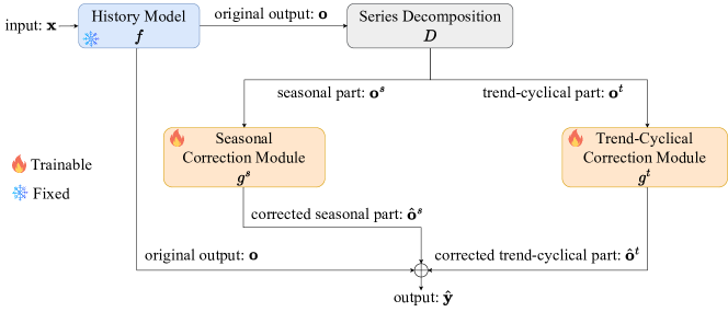
Figure 2: The framework of the proposed ADCSD method.

III-C Series Decomposition

For the OTTA of spatial-temporal traffic flow forecasting, we have access to a history model $f$ trained on the historical data and future data $\mathcal{X}$ need to be predicted. To correct the output of the history model, we take the idea of series decomposition [23], which can separate time series data into trend-cyclical and seasonal parts to learn complex temporal patterns in long-term forecasting. Specifically, for future data $\mathbf{x}$, we first obtain the output $\mathbf{o}$ of the history model $f$ as

$$\mathbf{o}=f(\mathbf{x}).$$ (1)

Then, to correct the output, we first decompose the output into seasonal and trend-cyclical parts by series decomposition. In detail, we first obtain the trend-cyclical part $\mathbf{o}^{t}$ of the original output via moving average as

$$\mathbf{o}^{t}=\text{AvgPool}(\text{Padding}(\mathbf{o})),$$

where $\text{AvgPool}(\cdot)$ denotes the average pooling operation on the time dimension and $\text{Padding}(\cdot)$ denotes the padding operation that is used to keep the length unchanged. Then the seasonal part $\mathbf{o}^{s}$ is equal to the difference between the original output and the trend-cyclical part, i.e.,

$$\mathbf{o}^{s}=\mathbf{o}-\mathbf{o}^{t}.$$

In short, we use the following equation to denote the series decomposition as

$$\mathbf{o}^{s},\mathbf{o}^{t}=D(\mathbf{o}).$$ (2)

After the series decomposition, we can break down the task of correcting the original output into correcting its seasonal and trend-cyclical parts, respectively, which facilitates the overall correction process.

III-D Correction Modules

To overcome the temporal drift problem, two correction modules are adopted to correct the seasonal and trend-cyclical parts, respectively. Specifically, for the seasonal part, the correction module is defined as

$$\hat{\mathbf{o}}^{s}=g^{s}(\mathbf{o}^{s}),$$ (3)

where $\hat{\mathbf{o}}^{s}$ is the corrected seasonal part and $g^{s}$ denotes the seasonal correction module. The seasonal correction module used in our work is a neural network of two fully-connected layers with layer normalization [40] and Gaussian Error Linear Unit (GELU) [41] activation function in the middle. Similarly, for the trend-cyclical part, the correction module is defined as

$$\hat{\mathbf{o}}^{t}=g^{t}(\mathbf{o}^{t}),$$ (4)

where $\hat{\mathbf{o}}^{t}$ is the corrected trend-cyclical part and $g^{t}$ denotes the trend-cyclical correction module. The trend-cyclical correction module has the same architecture as the seasonal correction module. With the integration of these two correction modules, the proposed ADCSD method enables the adaptation of the output to effectively align with the distribution of future data. By dynamically adjusting the model’s predictions based on the characteristics of the incoming data, we can enhance its ability to accurately capture the evolving patterns and trends present in the spatial-temporal domain. This adaptability ensures that our method remains robust and performs well when the data distribution changes over time.

III-E Adaptive Combination

Previous works [3, 8, 10] have shown that the relationship between different nodes is dynamic but not static. However, the mechanisms they employed to model the interaction of spatial information between nodes, such as graph neural networks or spatial attentions, are relatively heavyweight due to matrix multiplications involved. Moreover, since different nodes may have different levels of temporal drift and a shared module has difficulty in learning the different levels of temporal drift among different time series. To address these challenges, we adopt a lightweight approach that includes the introduction of two adaptive vectors. These vectors serve to implicitly incorporate the interaction of spatial information between traffic nodes and assign varying weights to different nodes in the corrected seasonal and trend-cyclical components, respectively, when combining them with the original output. Formally, let $\bm{\lambda}^{s}\in\mathbb{R}^{N}$ denote the seasonal adaptive vector and $\bm{\lambda}^{t}\in\mathbb{R}^{N}$ denote the trend-cyclical adaptive vector. The final output $\hat{\mathbf{y}}$ of our method is given as:

$$\hat{\mathbf{y}}=\mathbf{o}+\bm{\lambda}^{s}\hat{\mathbf{o}}^{s}+\bm{\lambda}^{t}\hat{\mathbf{o}}^{t}.$$ (5)

By utilizing those two trainable vectors, we are able to learn different weights for different nodes for the corrected seasonal and trend-cyclical parts, respectively, when combining them with the original output. Finally, the objective function of the proposed ADCSD method is formulated as:

$$\min_{g^{s},g^{t},\bm{\lambda}^{s},\bm{\lambda}^{t}}\ell(\mathbf{y},\hat{\mathbf{y}}),$$ (6)

where $\ell$ denotes the loss function such as the square loss. Note that parameters of the history model $f$ are fixed and we only update the parameters in correction modules $g^{s}$ and $g^{t}$ and adaptive vectors $\bm{\lambda}^{s}$ and $\bm{\lambda}^{t}$. The entire algorithm of the proposed ADCSD method is given in Algorithm 1.

Algorithm 1 Adaptive Double Correction by Series Decomposition

0:  history model $f$, future data $\mathcal{X}$;

1:  Randomly initialize $g^{s}$ and $g^{t}$;

2:  Initialize $\bm{\lambda}^{s}$ and $\bm{\lambda}^{t}$ as $\mathbf{0}$;

3:  for $t=1,\cdots,n$ do

4:     Compute the original output using Eq. (1);

5:     Decompose the original output into seasonal and trend-cyclical parts using Eq. (2);

6:     Correct the seasonal and trend-cyclical parts respectively using Eqs. (3) and (4);

7:     Compute the final output $\hat{\mathbf{y}}_{t}$ using Eq. (5);

8:     Update the parameters of $g^{s}$, $g^{t}$, $\bm{\lambda}^{s}$ and $\bm{\lambda}^{t}$ by minimizing problem (6);

9:  end for

III-F Analysis

For parameter efficiency, the proposed ADCSD method attaches a lite network including $g^{s}$ and $g^{t}$ behind the trained model and fine-tune the lite network. Here we provide some analyses to give insights into this method.

Let $\mathcal{X}=\{\mathbf{x}_{t},\mathbf{y}_{t}\}_{t=1}^{n}$ denotes the future traffic flow data, where $\mathbf{x}_{t}\in\mathbb{R}^{N\times T\times C}$ and $\mathbf{y}_{t}\in\mathbb{R}^{N\times T^{\prime}\times C}$. $f$ is the model trained on the historical data and the parameters are fixed during the testing phase. Let us consider two models. The output of model 1 is formulated as:

$$\hat{\mathbf{y}}=f(\mathbf{x}),$$ (7)

and that of model 2 is

$$\tilde{\mathbf{y}}=f(\mathbf{x})+g(f(\mathbf{x})),$$ (8)

where $g$ is the attached lite network. Hence, model 2 is just the proposed ADCSD method. We choose the square loss as the loss function for those two models and the loss function is defined as

$$\ell(\mathbf{y},\hat{\mathbf{y}})=\frac{1}{NT^{\prime}C}\sum_{i=1}^{NT^{\prime}C}(y_{i}-\hat{y}_{i})^{2},$$ (9)

where $y_{i}$ is the $i$-th component of $\mathbf{y}$ and $\hat{y}_{i}$ is the $i$-th component of $\hat{\mathbf{y}}$. For training losses of those two models, we have the following result.

Theorem 1.

We can find suitable function $g$ satisfying that the training loss of model 2 is lower than model 1, that is, we have

$$\ell(\mathbf{y},\tilde{\mathbf{y}})<\ell(\mathbf{y},\hat{\mathbf{y}}).$$ (10)

Proof.

Let $\ell(\mathbf{y},\hat{\mathbf{y}})=\frac{1}{NT^{\prime}C}\sum_{i=1}^{NT^{\prime}C}(y_{i}-\hat{y}_{i})^{2}=\frac{1}{NT^{\prime}C}\sum_{i=1}^{NT^{\prime}C}(y_{i}-f_{i}(\mathbf{x}))^{2}$, where $y_{i}$ is the $i$-th component of $\mathbf{y}$, $\hat{y}_{i}$ is the $i$-th component of $\hat{\mathbf{y}}$, and $f_{i}$ is the $i$-th component of function $f$. Similarly, $\ell(\mathbf{y},\tilde{\mathbf{y}})=\frac{1}{NT^{\prime}C}\sum_{i=1}^{NT^{\prime}C}(y_{i}-\tilde{y}_{i})^{2}=\frac{1}{NT^{\prime}C}\sum_{i=1}^{NT^{\prime}C}(y_{i}-f_{i}(\mathbf{x})-g_{i}(f(\mathbf{x})))^{2}$, where $\tilde{y}_{i}$ is the $i$-th component of $\tilde{\mathbf{y}}$, and $g_{i}$ is the $i$-th component of function $g$. Then we have

$$\begin{split}&NT^{\prime}C[\ell(\mathbf{y},\hat{\mathbf{y}})-\ell(\mathbf{y},\tilde{\mathbf{y}})]\\ =&\sum[(y_{i}-f_{i}(\mathbf{x}))^{2}-(y_{i}-f_{i}(\mathbf{x})-g_{i}(f(\mathbf{x})))^{2}]\\ =&\sum[y_{i}^{2}-2y_{i}f_{i}(\mathbf{x})+f^{2}_{i}(\mathbf{x})-(y_{i}^{2}+f^{2}_{i}(\mathbf{x})+g_{i}^{2}(f(\mathbf{x}))\\ &-2y_{i}f_{i}(\mathbf{x})-2y_{i}g_{i}(f(\mathbf{x}))+2f_{i}(\mathbf{x})g_{i}(f(\mathbf{x})))]\\ =&\sum[2y_{i}g_{i}(f(\mathbf{x}))-g_{i}^{2}(f(\mathbf{x}))-2f_{i}(\mathbf{x})g_{i}(f(\mathbf{x}))]\\ =&\sum g_{i}(f(\mathbf{x}))[2y_{i}-f_{i}(\mathbf{x})-g_{i}(f(\mathbf{x}))].\end{split}$$

Let $g_{i}(f(\mathbf{x}))=G_{i}$ and $2y_{i}-f_{i}(\mathbf{x})=C$, where $C$ is a constant since $g_{i}$ and $f_{i}$ are fixed for any given $i$. Then above equation becomes a function of $G_{i}$, i.e.,

$$G_{i}(C-G_{i}).$$

It is a conic and has two roots $G_{i}=0$ and $G_{i}=C$. By choosing suitable $G_{i}\in(0,C)$ or $(C,0)$, we can always have $\sum G_{i}(C-G_{i})>0$, which implies $\ell(\mathbf{y},\hat{\mathbf{y}})-\ell(\mathbf{y},\tilde{\mathbf{y}})>0$. ∎

Remark 1.

Theorem 1 implies that for a fixed model, attaching a lite trainable network will incur a lower training loss than that without the lite network. From the perspective of the model capacity, model 1 is a reduced version of model 2 by setting the parameters of the attached network to be zero and hence model 2 has a larger capacity than model 1, making model 2 possess a large chance to have a lower training loss. This conclusion is further verified in our experiments (i.e., Section IV-D).

To provide a theoretical analysis of the necessity of adding the original output to the final output. Let us consider the third model without the original output. Thus, the output of model 3 is formulated:

$$\bar{\mathbf{y}}=g(f(\mathbf{x})).$$ (11)

This model adopts the same loss function as models 1 and 2. For training losses of models 2 and 3, we have the following result.

Theorem 2.

We can find suitable function $g$ satisfying that the training loss of model 2 is lower than model 3, that is

$$\ell(\mathbf{y},\tilde{\mathbf{y}})<\ell(\mathbf{y},\bar{\mathbf{y}}).$$ (12)

Proof.

Let $\ell(\mathbf{y},\bar{\mathbf{y}})=\frac{1}{NT^{\prime}C}\sum_{i=1}^{NT^{\prime}C}(y_{i}-\bar{y}_{i})^{2}=\frac{1}{NT^{\prime}C}\sum_{i=1}^{NT^{\prime}C}(y_{i}-g_{i}(f(\mathbf{x})))^{2}$, where $y_{i}$ is the $i$-th component of $\mathbf{y}$, $\bar{y}_{i}$ is the $i$-th component of $\bar{\mathbf{y}}$, and $g_{i}$ is the $i$-th component of the function $g$. Similarly, $\ell(\mathbf{y},\tilde{\mathbf{y}})=\frac{1}{NT^{\prime}C}\sum_{i=1}^{NT^{\prime}C}(y_{i}-\tilde{y}_{i})^{2}=\frac{1}{NT^{\prime}C}\sum_{i=1}^{NT^{\prime}C}(y_{i}-f_{i}(\mathbf{x})-g_{i}(f(\mathbf{x})))^{2}$, where $\bar{y}_{i}$ is the $i$-th component of $\bar{\mathbf{y}}$, and $f_{i}$ is the $i$-th component of the function $f$. Then, in order to prove

$$\ell(\mathbf{y},\tilde{\mathbf{y}})<\ell(\mathbf{y},\bar{\mathbf{y}}).$$

We only need to prove

$$\ell(\mathbf{y},\bar{\mathbf{y}})-\ell(\mathbf{y},\tilde{\mathbf{y}})>0.$$

Then, we have

$$\small\begin{split}{}&NT^{\prime}C[\ell(\mathbf{y},\bar{\mathbf{y}})-\ell(\mathbf{y},\tilde{\mathbf{y}})]\\ =&\sum[(y_{i}-g_{i}(f(\mathbf{x})))^{2}-(y_{i}-f_{i}(\mathbf{x})-g_{i}(f(\mathbf{x})))^{2}]\\ =&\sum[y_{i}^{2}-2y_{i}g_{i}(f(\mathbf{x}))+g_{i}^{2}(f(\mathbf{x}))-(y_{i}^{2}+f^{2}_{i}(\mathbf{x})+g_{i}^{2}(f(\mathbf{x}))\\ &-2y_{i}f_{i}(\mathbf{x})-2y_{i}g_{i}(f(\mathbf{x}))+2f_{i}(\mathbf{x})g_{i}(f(\mathbf{x})))]\\ =&\sum[2y_{i}f_{i}(\mathbf{x})-f_{i}^{2}(\mathbf{x})-2f_{i}(\mathbf{x})g_{i}(f(\mathbf{x}))]\\ =&\sum f_{i}(\mathbf{x})[-f_{i}(\mathbf{x})+2y_{i}-2g_{i}(f(\mathbf{x}))].\end{split}$$

Since $y_{i}$ and $f_{i}(\cdot)$ are fixed for any given $i$, by choosing $g$, we can make $f_{i}(\mathbf{x})$ and $[-f_{i}(\mathbf{x})+2y_{i}-2g_{i}(f(\mathbf{x}))$ have the same symbol, i.e.,

$$f_{i}(\mathbf{x})[-f_{i}(\mathbf{x})+2y_{i}-2g_{i}(f(\mathbf{x}))]>0.$$

Thus, we have $\sum f_{i}(\mathbf{x})[-f_{i}(\mathbf{x})+2y_{i}-2g_{i}(f(\mathbf{x}))]>0$, which demonstrates $\ell(\mathbf{y},\bar{\mathbf{y}})-\ell(\mathbf{y},\tilde{\mathbf{y}})>0$. ∎

Remark 2.

Theorem 2 proves the importance and necessity of adding the original output, which is also demonstrated in our experiments (i.e., Section IV-D).

IV Experiments

IV-A Datasets

TABLE I: Statistics of Datasets.

Datasets	#Nodes	#Time Interval	#Input Window	#Output Window	Train:Val:Test	Time Range
PeMS07	883	5min	12	12	6:2:2	05/01/2017-08/31/2017
BayArea	699	5min	12	12	5:2:3	01/01/2019-12/30/2019
NYCTaxi	75 (15x5)	30min	6	6	7:1:2	01/01/2014-12/31/2014
T-Drive	1024 (32x32)	60min	6	6	7:1:2	02/01/2015-06/30/2015

We evaluate the proposed ADCSD method on four real-world public spatial-temporal traffic datasets, including two graph-based highway traffic datasets, i.e., PeMS07 [42], BayArea, and two grid-based citywide traffic datasets, i.e., NYCTaxi [43], T-Drive [44].

PeMS07 is collected from the Performance Measurement System (PeMS) of California Transportation Agencies (CalTrans) [45]. It is collected from 883 sensors installed in the California with observations of 4 months of data ranging from May 1 to August 31, 2017.

BayArea is also collected from PeMS of CalTrans. It is collected from 4096 sensors installed in the Bay Area with observations of 12 months of data ranging from January 1 to December 30, 2019. Then we discard the data of nodes with a missing rate greater than 0.1%, leaving only 699 nodes.

NYCTaxi is a dataset of taxi trips made in New York City. It is provided by the New York City Taxi and Limousine Commission (TLC). The data used in our paper spans from January 1 to December 31, 2014.

T-Drive is a dataset based on taxi GPS trajectories on Beijing, jointly released by Microsoft Asia Research Institute and Peking University. The data used in our paper spans from February 1 to June 30, 2015.

The graph-based datasets contain only the traffic flow data, and the grid-based datasets contain inflow and outflow data. More details about these datasets used in our paper are given in Table I. Note that the training and validation sets are regarded as historical data to train the model, and the test sets are regarded as future data.

IV-B Experimental Settings

IV-B1 Baselines

To validate the correctness and effectiveness of our method, we plug-and-play our method after several commonly used traffic flow traffic forecasting models, including ASTGCN [7], AGCRN [8] and PDFormer [10]. To the best of our knowledge, there is no comparable method for OTTA of spatial-temporal traffic flow forecasting. Thus, we reimplement several OTTA methods used in computer vision area for spatial-temporal traffic flow forecasting, including TENT [17] and TTT-MAE [18].

IV-B2 Implementation details

All the baseline models (i.e, ASTGCN, AGCRN and PDFormer) are implemented based on the LibCity library [46]. The seasonal and trend-cyclical correction modules have the same architecture, i.e., two fully connected layers with Layer Normalization [40] and Gaussian Error Linear Unit (GELU) [41] activation function in the middle. For training the history models, we follow the optimization details in their original paper. The optimal history model is determined based on the performance in the validation set. For testing phase, we optimize the correction modules with the Adam [47] optimizer with an initial learning rate of $10^{-4}$. Both the epoch and batch size are set to one to follow the online learning setting. All the experiments are conducted on Tesla A100 GPUs.

IV-B3 Evaluation Metrics

We use three metrics in the experiments: (1) Mean Absolute Error (MAE), (2) Mean Absolute Percentage Error (MAPE), and (3) Root Mean Squared Error (RMSE). Missing values are excluded when calculating these metrics. When we test the models on the grid-based datasets, we filter the samples with flow values below 10, consistent with [10].

IV-C Main Results

TABLE II: Performance on the graph-based datasets. A lower MSE, MAPE, or MAE indicates better performance, and the best results are highlighted in bold.

	Fine-tune method	PeMS07			BayArea
		MAE	MAPE(%)	RMSE	MAE	MAPE(%)	RMSE
ASTGCN	Test	23.708	10.170	36.903	19.201	10.531	31.678
	TENT [17]	33.196	18.407	50.396	21.857	13.057	33.861
	TTT-MAE [18]	32.306	15.635	46.456	20.757	12.154	32.697
	ADCSD	22.910	9.975	35.740	17.380	9.536	29.111
AGCRN	Test	20.700	8.980	34.338	17.169	9.609	30.632
	TENT [17]	54.461	36.299	81.075	53.596	39.067	76.288
	TTT-MAE [18]	31.565	15.838	45.101	22.484	13.731	35.292
	ADCSD	20.211	8.623	33.389	15.507	8.542	27.706
PDFormer	Test	19.802	8.565	32.820	14.883	7.673	27.866
	TENT [17]	23.020	11.483	35.369	20.823	14.907	31.790
	TTT-MAE [18]	20.051	8.706	33.012	15.409	8.430	27.978
	ADCSD	19.627	8.393	32.607	14.667	7.617	27.531

IV-C1 Graph-based Datasets

The comparison results with baselines of different models on the graph-based datasets are shown in Table II. Based on this table, we can make the following observations. (1) OTTA from CV cannot be reused directly: The performance of OTTA methods proposed in the computer vision area (i.e., TENT and TTT-MAE) are inferior to the original trained model (i.e., the Test method), which means these methods do not work in the spatial-temporal traffic flow forecasting problem. Thus, it is necessary to design new algorithm according to the characteristics of traffic flow data when applying OTTA to spatial-temporal traffic flow forecasting. (2) Fine-tuning not always works: The performance of TENT drops dramatically compared with the original trained model, which indicates fine-tuning all the parameters of the trained model is not a good choice for the online spatial-temporal traffic flow forecasting problem. (3) Effectiveness of ADCSD: Our proposed method ADCSD can further improve the performance of the trained models and achieve the best results on all datasets, which demonstrates the effectiveness and stability of our method. The incorporation of learnable components enables the proposed ADCSD method to gradually adapt and learn towards the future data distribution, thereby alleviating the issue of temporal drift.

TABLE III: Performance on the grid-based datasets. A lower MSE, MAPE, or MAE indicates better performance, and the best results are highlighted in bold.

		NYCTaxi						T-Drive
	Fine-tune Method	inflow			outflow			inflow			outflow
		MAE	MAPE(%)	RMSE	MAE	MAPE(%)	RMSE	MAE	MAPE(%)	RMSE	MAE	MAPE(%)	RMSE
ASTGCN	Test	25.302	23.405	43.228	21.720	22.515	37.758	41.578	32.410	76.801	41.376	32.385	76.365
	TENT [17]	26.915	27.290	43.592	24.436	29.276	39.502	54.139	45.236	95.186	54.154	45.689	95.185
	TTT-MAE [18]	25.469	23.840	43.414	22.242	24.024	38.061	43.278	35.354	78.464	43.053	35.277	78.072
	ADCSD	25.117	23.280	42.941	21.480	22.487	37.315	41.499	32.328	76.675	41.248	32.299	76.166
AGCRN	Test	18.299	16.445	31.948	15.754	16.211	27.383	21.374	16.478	41.066	21.395	16.459	41.081
	TENT [17]	41.357	42.575	67.217	38.109	45.765	64.413	73.054	60.799	126.561	72.923	60.353	126.684
	TTT-MAE [18]	20.675	19.105	35.302	18.052	18.929	30.755	28.572	22.574	52.056	28.588	22.523	52.121
	ADCSD	18.114	16.232	31.673	15.569	16.001	27.102	21.242	16.389	40.856	21.271	16.366	40.897
PDFormer	Test	17.150	15.320	30.185	14.778	15.055	25.903	21.481	17.504	38.889	21.515	17.507	38.914
	TENT [17]	24.256	24.304	40.333	21.265	24.858	35.357	45.906	35.253	80.966	45.734	35.034	80.766
	TTT-MAE [18]	17.221	15.437	30.163	14.902	15.204	25.998	22.164	18.187	39.515	22.194	18.193	39.547
	ADCSD	16.987	15.181	29.928	14.595	14.912	25.460	21.308	17.283	38.664	21.337	17.274	38.694

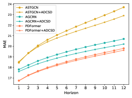
(a) MAE

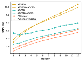
(b) MAPE

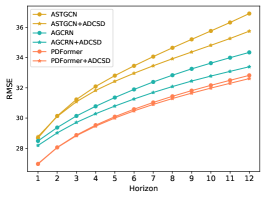
(c) RMSE

Figure 3: Prediction performance comparison at each horizon on the PeMS07 dataset.

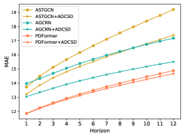
(a) MAE

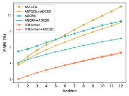
(b) MAPE

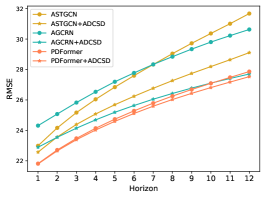
(c) RMSE

Figure 4: Prediction performance comparison at each horizon on the BayArea dataset.

Figure 3 further shows the prediction performance at each horizon on PeMS07. With our method attached behind, the performance of the trained models is further improved for almost all horizons, which indicates our method balances short-term and long-term prediction well. Furthermore, our method can achieve more improvement for long-term prediction compared with short-term prediction. This is because, with a longer prediction horizon, the data is more likely to drift away; thus our ADCSD shows its more correction ability from adaptively weighting the seasonal and trend-cyclical corrections. Figure 4 shows the prediction performance at each horizon on the BayArea dataset. Similar to the results on the PeMS07 dataset (see Figure 3), the performance of the trained models improve for almost all horizons with the incorporation of our method, which indicates our method balances short-term and long-term prediction well. In addition, compared to short-term prediction, our method is capable of achieving large improvement in long-term forecasting, which is similar to the phenomenon on the PeMS07 dataset (see Figure 3). Furthermore, our approach can achieve significant performance improvements when the performance of the original model is not so good.

IV-C2 Grid-based Datasets

The comparison results with different baselines in the grid-based datasets are shown in Table III. It can be seen from this table that there are the same experimental phenomena as on the graph-based datasets (i.e., Table II), but a slight difference. That is, no matter the performance of the original trained model is good or bad, our method has a stable and relatively obvious improvement, which is different from the phenomenon on the graph-based datasets that there is a higher improvement on models with poor performance and less improvement on models with good performance.

IV-D Ablation Study

To verify the effectiveness of each component in the proposed ADCSD model, we conduct a comprehensive ablation study on both graph-based and grid-based datasets.

IV-D1 Graph-based Datasets

Table IV shows ablation study of the graph-based datasets. The model M0 with only the original output $\mathbf{o}$ denotes the results of the model trained on the historical data without any modification. M5 denotes our method. M6 denotes no decomposition on time series. Based on these results, we can conclude the following: (1) Original output matters: According to the results between M1 and M2 ($+\mathbf{o}$), there is a significant decrease in performance when the original output is absent. This suggests that the original output plays a crucial role in achieving accurate predictions. (2) Adaptive vectors matter: By comparing M2 and M5 ($+\bm{\lambda}^{s},\bm{\lambda}^{t}$), we can see that the absence of adaptive vectors leads to a decrease in performance. This finding highlights the importance of adaptive vectors as a critical component of our method. That is because different nodes have different levels of temporal drift and it’s necessary to assign different weights to different nodes. (3) Decomposition matters: By comparing M5 and M6, we can see that the absence of decomposing time series leads to a decrease in performance, which indicates the decomposing strategy is helpful. Comparing M3-M5 with M0, we observe that correcting the seasonal or the trend-cyclical part separately can improve the performance, but combining both parts leads to a more significant enhancement in performance, which demonstrates both these two parts are crucial for the performance improvement of our method.

TABLE IV: Ablation study on the graph-based datasets.

	Method	$\mathbf{o}$	$\hat{\mathbf{o}}^{s}$	$\hat{\mathbf{o}}^{t}$	$\bm{\lambda}^{s}$	$\bm{\lambda}^{t}$	PeMS07			BayArea
							MAE	MAPE(%)	RMSE	MAE	MAPE(%)	RMSE
ASTGCN	M0	✓					23.708	10.170	36.903	19.201	10.531	31.678
	M1		✓	✓			30.277	20.902	48.528	21.158	15.264	33.164
	M2	✓	✓	✓			23.604	11.752	36.351	18.020	10.333	29.422
	M3	✓	✓		✓		23.329	10.193	36.213	18.220	10.432	30.022
	M4	✓		✓		✓	22.976	9.954	35.822	17.404	9.553	29.135
	M5	✓	✓	✓	✓	✓	22.910	9.975	35.740	17.380	9.536	29.111
	M6	$\hat{\mathbf{y}}=\mathbf{o}+\bm{\lambda}\hat{\mathbf{o}}$					23.077	10.045	36.034	18.031	9.763	29.899
AGCRN	M0	✓					20.700	8.980	34.338	17.169	9.609	30.632
	M1		✓	✓			28.495	22.191	45.410	19.076	14.359	30.887
	M2	✓	✓	✓			21.358	9.952	34.764	17.279	10.509	28.530
	M3	✓	✓		✓		20.433	8.784	33.723	16.181	9.273	28.634
	M4	✓		✓		✓	20.257	8.635	33.443	15.514	8.548	27.727
	M5	✓	✓	✓	✓	✓	20.211	8.623	33.389	15.507	8.542	27.706
	M6	$\hat{\mathbf{y}}=\mathbf{o}+\bm{\lambda}\hat{\mathbf{o}}$					20.404	8.681	33.777	16.033	9.025	28.334
PDFormer	M0	✓					19.802	8.565	32.820	14.883	7.673	27.866
	M1		✓	✓			24.346	17.619	37.270	17.219	10.399	29.526
	M2	✓	✓	✓			20.053	9.141	32.855	15.567	8.419	27.707
	M3	✓	✓		✓		19.715	8.474	32.689	14.786	7.699	27.717
	M4	✓		✓		✓	19.654	8.447	32.634	14.670	7.618	27.535
	M5	✓	✓	✓	✓	✓	19.627	8.393	32.607	14.667	7.617	27.531
	M6	$\hat{\mathbf{y}}=\mathbf{o}+\bm{\lambda}\hat{\mathbf{o}}$					19.717	8.448	32.688	14.677	7.620	27.633

TABLE V: Ablation study on the grid-based datasets.

							NYCTaxi						T-Drive
	Method	$\mathbf{o}$	$\hat{\mathbf{o}}^{s}$	$\hat{\mathbf{o}}^{t}$	$\bm{\lambda}^{s}$	$\bm{\lambda}^{t}$	inflow			outflow			inflow			outflow
							MAE	MAPE(%)	RMSE	MAE	MAPE(%)	RMSE	MAE	MAPE(%)	RMSE	MAE	MAPE(%)	RMSE
ASTGCN	M0	✓					25.302	23.405	43.228	21.720	22.515	37.758	41.578	32.410	76.801	41.376	32.385	76.365
	M1		✓	✓			31.368	31.479	57.114	28.392	31.418	51.594	72.957	65.586	140.727	68.760	45.872	130.298
	M2	✓	✓	✓			25.401	24.403	42.942	22.802	26.713	37.940	42.843	37.484	77.629	47.784	49.342	81.590
	M3	✓	✓		✓		25.204	23.339	43.164	21.563	22.521	37.611	41.529	32.395	76.740	41.313	32.388	76.283
	M4	✓		✓		✓	25.133	23.252	42.991	21.547	22.523	37.446	41.523	32.348	76.694	41.294	32.322	76.207
	M5	✓	✓	✓	✓	✓	25.117	23.280	42.941	21.480	22.487	37.315	41.499	32.328	76.675	41.248	32.299	76.166
	M6	$\hat{\mathbf{y}}=\mathbf{o}+\bm{\lambda}\hat{\mathbf{o}}$					25.131	23.316	42.941	21.559	22.586	37.428	41.503	32.388	76.786	41.332	32.315	76.223
AGCRN	M0	✓					18.299	16.445	31.948	15.754	16.211	27.383	21.374	16.478	41.066	21.395	16.459	41.081
	M1		✓	✓			25.553	25.020	48.699	21.324	25.699	37.104	59.871	53.029	109.597	61.660	36.773	136.090
	M2	✓	✓	✓			18.611	17.605	31.971	16.551	18.166	28.632	33.591	49.569	52.663	29.340	36.276	52.176
	M3	✓	✓		✓		18.195	16.289	31.807	15.649	16.077	27.210	21.285	16.411	40.983	21.307	16.393	41.003
	M4	✓		✓		✓	18.125	16.270	31.679	15.591	16.018	27.138	21.263	16.411	40.879	21.306	16.397	40.940
	M5	✓	✓	✓	✓	✓	18.114	16.232	31.673	15.569	16.001	27.102	21.242	16.389	40.856	21.271	16.366	40.897
	M6	$\hat{\mathbf{y}}=\mathbf{o}+\bm{\lambda}\hat{\mathbf{o}}$					18.114	16.326	31.691	15.621	16.129	27.112	21.304	16.447	41.053	21.338	16.406	41.092
PDFormer	M0	✓					17.150	15.320	30.185	14.778	15.055	25.903	21.481	17.504	38.889	21.515	17.507	38.914
	M1		✓	✓			30.361	28.484	66.836	24.893	27.800	55.012	76.860	51.039	174.795	74.451	47.152	164.612
	M2	✓	✓	✓			18.901	18.371	32.556	16.835	19.531	28.490	26.191	21.729	46.951	31.702	29.496	54.644
	M3	✓	✓		✓		17.069	15.274	30.034	14.731	15.035	25.727	21.395	17.411	38.821	21.417	17.403	38.832
	M4	✓		✓		✓	16.999	15.189	29.941	14.608	14.919	25.487	21.343	17.327	38.674	21.379	17.324	38.709
	M5	✓	✓	✓	✓	✓	16.987	15.181	29.928	14.595	14.912	25.460	21.308	17.283	38.664	21.337	17.274	38.694
	M6	$\hat{\mathbf{y}}=\mathbf{o}+\bm{\lambda}\hat{\mathbf{o}}$					17.001	15.201	30.020	14.673	14.976	25.653	21.412	17.529	38.715	21.412	17.493	38.701

IV-D2 Grid-based Datasets

Experimental results of ablation study on the grid-based datasets are shown in Table V. The phenomena are similar to the results on the graph-based dataset (see Table IV). That is, (1) Original output matters: The original output plays a crucial role in achieving accurate predictions. (2) Adaptive vectors matter: The adaptive vectors are a critical component of our method. (3) Decomposition matters: The decomposing strategy is helpful. Both the seasonal and trend-cyclical parts are crucial to the performance improvement of our method.

TABLE VI: Computational cost on the NYCTaxi dataset.

Method	ASTGCN		AGCRN		PDFormer
	# Parameters	# Time	# Parameters	# Time	# Parameters	# Time
Test	-	43s	-	35s	-	63s
TENT [17]	72542	133s	750330	127s	531628	307s
TTT-MAE [18]	72542	144s	750330	128s	531628	344s
ADCSD	231834	97s	231834	76s	231834	132s

IV-E Computational Cost

To evaluate the computational cost, we compare the parameter numbers and testing time of our method with TENT and TTT-MAE on the NYCTaxi dataset in Table VI. In terms of the training time, our method runs faster than all compared baseline methods and only slightly slower than the direct test method, which demonstrates the efficiency of our method. Furthermore, the training parameters of our method are less than OTTA baselines when the trained model is AGCRN or PDFormer. That is because the training parameters of baselines are related to the trained model. The more parameters of the trained model, the more parameters baselines are required, while the parameters of our method are fixed and kept at a small value.

V Conclusion

In this paper, to tackle the temporal drift problem in spatial-temporal traffic flow forecasting, we conduct the first study to apply OTTA to the spatial-temporal traffic flow forecasting problem. In order to adapt to the characteristics of traffic flow data, we propose the ADCSD model, which first decomposes the output of a trained model into seasonal and trend-cyclical parts and then corrects them by two separate modules during the testing phase using the latest observed data. Based on this operation, the model trained on the historical data can better adapt to future data. The proposed method is a lite network that can be universally attached with main-stream traffic flow forecasting deep models as a plug-and-play component, and it could significantly improve their performance. Applying OTTA to spatial-temporal traffic flow forecasting to solve the temporal drift problem is practical since it fits the characteristics of time series data, and we hope more researchers can pay attention to this practical setting. In our future study, we are interested in applying the proposed ADCSD model to more applications in intelligent transportation.

References

- [1] X. Liu, X. Qin, M. Zhou, H. Sun, and S. Han, “Community-based dandelion algorithm-enabled feature selection and broad learning system for traffic flow prediction,” IEEE Trans. Intell. Transp. Syst., pp. 1–14, 2023.
- [2] Y. Lv, Y. Duan, W. Kang, Z. Li, and F.-Y. Wang, “Traffic flow prediction with big data: A deep learning approach,” IEEE Trans. Intell. Transp. Syst., vol. 16, no. 2, pp. 865–873, 2014.
- [3] L. Zhao, Y. Song, C. Zhang, Y. Liu, P. Wang, T. Lin, M. Deng, and H. Li, “T-gcn: A temporal graph convolutional network for traffic prediction,” IEEE Trans. Intell. Transp. Syst., vol. 21, no. 9, pp. 3848–3858, 2019.
- [4] D. A. Tedjopurnomo, Z. Bao, B. Zheng, F. M. Choudhury, and A. K. Qin, “A survey on modern deep neural network for traffic prediction: Trends, methods and challenges,” IEEE Trans. Knowl. Data Eng., vol. 34, no. 4, pp. 1544–1561, 2020.
- [5] W. Jiang and J. Luo, “Graph neural network for traffic forecasting: A survey,” Expert Syst. Appl., vol. 207, p. 117921, 2022.
- [6] A. M. Nagy and V. Simon, “Survey on traffic prediction in smart cities,” Pervasive Mob. Comput., vol. 50, pp. 148–163, 2018.
- [7] S. Guo, Y. Lin, N. Feng, C. Song, and H. Wan, “Attention based spatial-temporal graph convolutional networks for traffic flow forecasting,” in Proc. AAAI Conf. Artif. Intell., vol. 33, no. 01, 2019, pp. 922–929.
- [8] L. Bai, L. Yao, C. Li, X. Wang, and C. Wang, “Adaptive graph convolutional recurrent network for traffic forecasting,” Proc. Adv. Neural Inf. Process. Syst. (NeurIPS), vol. 33, pp. 17 804–17 815, 2020.
- [9] G. Woo, C. Liu, D. Sahoo, A. Kumar, and S. Hoi, “Cost: Contrastive learning of disentangled seasonal-trend representations for time series forecasting,” in Proc. Int. Conf. Learn. Represent. (ICLR), 2022.
- [10] J. Jiang, C. Han, W. X. Zhao, and J. Wang, “Pdformer: Propagation delay-aware dynamic long-range transformer for traffic flow prediction,” in Proc. AAAI Conf. Artif. Intell., 2023.
- [11] V. Kuznetsov and M. Mohri, “Generalization bounds for time series prediction with non-stationary processes,” in Proc. Algorithmic Learning Theory (ALT), 2014, pp. 260–274.
- [12] Y. Du, J. Wang, W. Feng, S. Pan, T. Qin, R. Xu, and C. Wang, “Adarnn: Adaptive learning and forecasting of time series,” in Proc. Conf. Inf. Know. Mana. (CIKM), 2021, pp. 402–411.
- [13] W. Duan, X. He, L. Zhou, L. Thiele, and H. Rao, “Combating distribution shift for accurate time series forecasting via hypernetworks,” in Proc. Int. Conf. Para. Dist. Syst. (ICPADS). IEEE, 2023, pp. 900–907.
- [14] J. Liang, R. He, and T. Tan, “A comprehensive survey on test-time adaptation under distribution shifts,” Preprint arXiv:2303.15361, 2023.
- [15] Y. Sun, X. Wang, Z. Liu, J. Miller, A. Efros, and M. Hardt, “Test-time training with self-supervision for generalization under distribution shifts,” in Proc. Int. Conf. Mach. Learn. (ICML). PMLR, 2020, pp. 9229–9248.
- [16] S. Niu, J. Wu, Y. Zhang, Y. Chen, S. Zheng, P. Zhao, and M. Tan, “Efficient test-time model adaptation without forgetting,” in Proc. Int. Conf. Mach. Learn. (ICML). PMLR, 2022, pp. 16 888–16 905.
- [17] D. Wang, E. Shelhamer, S. Liu, B. Olshausen, and T. Darrell, “Tent: Fully test-time adaptation by entropy minimization,” in Proc. Int. Conf. Learn. Represent. (ICLR), 2021.
- [18] Y. Gandelsman, Y. Sun, X. Chen, and A. Efros, “Test-time training with masked autoencoders,” Proc. Adv. Neural Inf. Process. Syst. (NeurIPS), vol. 35, pp. 29 374–29 385, 2022.
- [19] T. Gong, J. Jeong, T. Kim, Y. Kim, J. Shin, and S.-J. Lee, “Note: Robust continual test-time adaptation against temporal correlation,” Proc. Adv. Neural Inf. Process. Syst. (NeurIPS), vol. 35, pp. 27 253–27 266, 2022.
- [20] Q. Wang, O. Fink, L. Van Gool, and D. Dai, “Continual test-time domain adaptation,” in Proc. IEEE/CVF Conf. Comput. Vis. Pattern Recognit. (CVPR), 2022, pp. 7201–7211.
- [21] C. Tian and W. K. Chan, “Spatial-temporal attention wavenet: A deep learning framework for traffic prediction considering spatial-temporal dependencies,” IET Intell. Transp. Syst., vol. 15, no. 4, pp. 549–561, 2021.
- [22] K. Clark, K. Guu, M.-W. Chang, P. Pasupat, G. Hinton, and M. Norouzi, “Meta-learning fast weight language models,” Preprint arXiv:2212.02475, 2022.
- [23] R. B. Cleveland, W. S. Cleveland, J. E. McRae, and I. Terpenning, “Stl: A seasonal-trend decomposition,” J. Off. Stat., vol. 6, no. 1, pp. 3–73, 1990.
- [24] R. J. Hyndman and G. Athanasopoulos, Forecasting: principles and practice. OTexts, 2018.
- [25] Z. Li, H. Yan, C. Zhang, and F. Tsung, “Long-short term spatiotemporal tensor prediction for passenger flow profile,” IEEE Robot. Autom. Lett., vol. 5, no. 4, pp. 5010–5017, 2020.
- [26] F. Amato, F. Guignard, S. Robert, and M. Kanevski, “A novel framework for spatio-temporal prediction of environmental data using deep learning,” Sci Rep, vol. 10, no. 1, p. 22243, 2020.
- [27] D. Liu, J. Wang, S. Shang, and P. Han, “Msdr: Multi-step dependency relation networks for spatial temporal forecasting,” in Proc. SIGKDD Conf. Know. Disc. & Data Mining, 2022, pp. 1042–1050.
- [28] N. Jones, “How machine learning could help to improve climate forecasts,” Nature, vol. 548, no. 7668, 2017.
- [29] A. Longo, M. Zappatore, M. Bochicchio, and S. B. Navathe, “Crowd-sourced data collection for urban monitoring via mobile sensors,” ACM Trans. Internet. Technol., vol. 18, no. 1, pp. 1–21, 2017.
- [30] S. Guo, Y. Lin, H. Wan, X. Li, and G. Cong, “Learning dynamics and heterogeneity of spatial-temporal graph data for traffic forecasting,” IEEE Trans. Knowl. Data Eng., vol. 34, no. 11, pp. 5415–5428, 2021.
- [31] X. You, M. Zhang, D. Ding, F. Feng, and Y. Huang, “Learning to learn the future: Modeling concept drifts in time series prediction,” in Proc. Conf. Inf. Know. Mana. (CIKM), 2021, pp. 2434–2443.
- [32] S. O. Arik, N. C. Yoder, and T. Pfister, “Self-adaptive forecasting for improved deep learning on non-stationary time-series,” Preprint arXiv:2202.02403, 2022.
- [33] T. Kim, J. Kim, Y. Tae, C. Park, J.-H. Choi, and J. Choo, “Reversible instance normalization for accurate time-series forecasting against distribution shift,” in Proc. Int. Conf. Learn. Represent. (ICLR), 2022.
- [34] R. Wang, Y. Dong, S. O. Arik, and R. Yu, “Koopman neural operator forecaster for time-series with temporal distributional shifts,” in Proc. Int. Conf. Learn. Represent. (ICLR), 2023.
- [35] G. Bai, C. Ling, and L. Zhao, “Temporal domain generalization with drift-aware dynamic neural networks,” in Proc. Int. Conf. Learn. Represent. (ICLR), 2023.
- [36] X. Hu, G. Uzunbas, S. Chen, R. Wang, A. Shah, R. Nevatia, and S.-N. Lim, “Mixnorm: Test-time adaptation through online normalization estimation,” Preprint arXiv:2110.11478, 2021.
- [37] F. Azimi, S. Palacio, F. Raue, J. Hees, L. Bertinetto, and A. Dengel, “Self-supervised test-time adaptation on video data,” in Proc. IEEE/CVF Int. Conf. Comput. Vis. (ICCV), 2022, pp. 3439–3448.
- [38] J. Hong, L. Lyu, J. Zhou, and M. Spranger, “Mecta: Memory-economic continual test-time model adaptation,” in Proc. Int. Conf. Learn. Represent. (ICLR), 2023.
- [39] M. Boudiaf, R. Mueller, I. Ben Ayed, and L. Bertinetto, “Parameter-free online test-time adaptation,” in Proc. IEEE/CVF Conf. Comput. Vis. Pattern Recognit. (CVPR), 2022, pp. 8344–8353.
- [40] J. L. Ba, J. R. Kiros, and G. E. Hinton, “Layer normalization,” Preprint arXiv:1607.06450, 2016.
- [41] D. Hendrycks and K. Gimpel, “Gaussian error linear units (gelus),” Preprint arXiv:1606.08415, 2016.
- [42] C. Song, Y. Lin, S. Guo, and H. Wan, “Spatial-temporal synchronous graph convolutional networks: A new framework for spatial-temporal network data forecasting,” in Proc. AAAI Conf. Artif. Intell., vol. 34, no. 01, 2020, pp. 914–921.
- [43] L. Liu, J. Zhen, G. Li, G. Zhan, Z. He, B. Du, and L. Lin, “Dynamic spatial-temporal representation learning for traffic flow prediction,” IEEE Trans. Intell. Transp. Syst., vol. 22, no. 11, pp. 7169–7183, 2020.
- [44] Z. Pan, Y. Liang, W. Wang, Y. Yu, Y. Zheng, and J. Zhang, “Urban traffic prediction from spatio-temporal data using deep meta learning,” in Proc. SIGKDD Conf. Know. Disc. & Data Mining, 2019, pp. 1720–1730.
- [45] C. Chen, K. Petty, A. Skabardonis, P. Varaiya, and Z. Jia, “Freeway performance measurement system: mining loop detector data,” Transp. Res. Record, vol. 1748, no. 1, pp. 96–102, 2001.
- [46] J. Wang, J. Jiang, W. Jiang, C. Li, and W. X. Zhao, “Libcity: An open library for traffic prediction,” in Proc. ACM SIGSPATIAL Conf., 2021, pp. 145–148.
- [47] D. P. Kingma and J. Ba, “Adam: A method for stochastic optimization,” Preprint arXiv:1412.6980, 2014.