Robust Calibration For Improved Weather Prediction Under Distributional Shift

Abstract

In this paper, we present results on improving out-of-domain weather prediction and uncertainty estimation as part of the Shifts Challenge on Robustness and Uncertainty under Real-World Distributional Shift challenge. We find that by leveraging a mixture of experts in conjunction with an advanced data augmentation technique borrowed from the computer vision domain, in conjunction with robust post-hoc calibration of predictive uncertainties, we can potentially achieve more accurate and better-calibrated results with deep neural networks than with boosted tree models for tabular data. We quantify our predictions using several metrics and propose several future lines of inquiry and experimentation to boost performance.

1 Introduction

Machine learning is increasingly being applied across several domains, finding ever new applications in the real world, in fields ranging from astrophysics (Gilda et al., 2018; Gilda, 2023b, a; Dainotti et al., 2019; Gilda et al., 2021c, d, e; Narayanan et al., 2021; Gilda, 2019b), to recommendations systems (Aher and Lobo, 2013; Doshi et al., 2018; Portugal et al., 2018), to drug discovery (Lavecchia, 2015; Vamathevan et al., 2019; Zhang et al., 2017). A key assumption held by several of these models is that training and test data are independent and identically distributed (IID); this assumption rarely holds up to scrutiny in the real-world, where the models must process unseen and unpredictable distributions. This leads to several machine learning models providing unsatisfactory performance in production. The development of models that are robust to distributional shifts, therefore, is an important goal to work towards.

A prime exemplar for a field where distributional shifts are abundant over time is weather prediction. Weather prediction requires that models provide consistently satisfactory performance across both as a function of space (latitude, longitude, climate) and time (of day, month, year). Due to geographical and population constraints, the distribution of weather recording services is non-uniform in nature. While there have been several works in the field of weather prediction, the Shifts Challenge on Robustness and Uncertainty under Real-World Distributional Shift presents a unique opportunity to develop and apply models that are robust to such effects and also yield sensible uncertainty estimates. We present here an empirical study on the effects of regularization, calibration, and data augmentation in a multi-domain training environment.

Our main contributions are thus. First, we leverage a mixture density network (MDN, Bishop, 1994; Choi et al., 2017; Gilda et al., 2021b, 2020) with $\beta-$likelihoods and demonstrate competitive performance relative to two commonly used boosted-tree models, NGBoost (Duan et al., 2020) and CatBoost (Prokhorenkova et al., 2019). Second, we demonstrate the necessity of regularization while training the MDN. Specifically, we use moment exchange (MoEx, Li et al., 2021), a data augmentation method originally developed for use in computer vision (CV), to regularize our MDN successfully. Third, we demonstrate the necessity of calibrating predictions, and utilize a state-of-the-art post-hoc calibration method (CRUDE, Zelikman et al., 2020) to that end. Fourth, we illustrate that the inverse variance weighing method, commonly used to combine predictions from members of an ensemble, improves predicted means but results in poorly calibrated uncertainties. Finally, we demonstrate, for the first time with a tabular dataset, the improvement in predicted negative log likelihood (NLL) resulting from robust, domain-aware calibration (Wald et al., 2021).

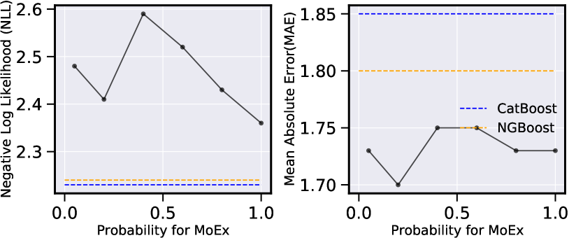
Figure 1: Impact of varying the probability parameter p in MoEx. p is the probability that a given sample will be augmented. Left: Negative log likelihood of robust, post-hoc predictions on TEST vs. p and mean absolute error. Right: Mean absolute error instead of NLL. For both plots, lower is better. We denote by dashed orange and blue lines the respective predicted metrics from NGBoost and CatBoost (see last lines in Tables 2 and 3, respectively).

2 Data

We employ the Weather Prediction dataset developed by Yandex Research for the Shifts Challenge. This dataset comprises several meteorological features from three major global weather prediction models, as well as air temperatures 2 metres above ground (fact_temperature), for a diverse set of latitudes and longitudes. The goal of this competition is to predict air temperature at 2 meters above ground, given all available weather station measurements and multiple weather forecast model predictions. While the training data has information about location on earth and the timestamp when predictions from the 3 global forecasting systems were made, these meta-data are assumed to be missing for the test set.

There are two specific set of feature categories that make up this dataset: weather-related features and meteorological features. Weather related features consist of sun evaluation at the current location, climate values of temperature, pressure and topography. Meteorological parameters are details based on pressure and surface level data from the weather prediction models. There are five climate types associated with the data: Tropical, Dry, Mild Temperate, Snow and Polar. The data are split into training, development and evaluation sets based on the climate and time of year, in order to provide a clear distributional shift in the weather data. The development set is first sub-divided into ID-development and OoD-development (in-distribution an out of distribution, respectively), and is designed to simulate the evaluation set. In this paper, we only use the first two datasets as these were the only ones released during the first phase of the competition. The training data consists of features with climate types as Tropical, Dry and Mild Temperature. This data is recorded from the $1^{st}$ of September 2018, to the $8^{th}$ of April, 2019. dev-ID has the same climate types and time of year (first and last thirds of the year) as the training data, whereas dev-OoD consists of samples only with the climate type Snow, and during the middle third of the year. The evaluation dataset, of course, has been shifted based on climate and time. It consists of features with Snow and Polar climate types, recorded from the $14^{th}$ May, 2019 to the $8^{th}$ of July,2019. The training, dev-ID and dev-OoD datasets show a clear distributional shift, presenting a challenge to develop models robust to these shifts and competent at generalisation to OoD data in the real world.

3 Method

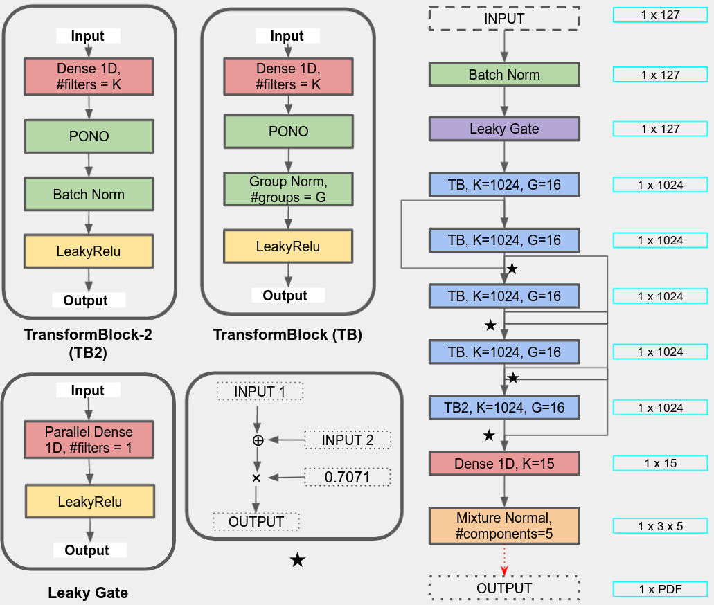
Figure 2: Architecture of the mixture density network (MDN, Bishop, 1994; Choi et al., 2017). PONO is the positional normalization layer Li et al. (2019), and the use of LeakyGate is inspired by Fiedler (2021). We model the output variable fact_temperature conditioned on the input variables using a mixture of 5 $\beta$ distributions.

1. We divide the given training dataset T_ALL with $\sim$3.1 million samples into six disjoint datasets ($\texttt{T\_E}1$, $\texttt{T\_E}2$, $\texttt{T\_E}3$, $\texttt{T\_E}4$, $\texttt{T\_E}5$, and $\texttt{T\_E}6$) based on climate and week_of_year. We use the ID part of the development dataset as our validation data V_ALL, and the OoD part as the test set TEST. We divide the former it into $\texttt{V\_E}1$, $\texttt{V\_E}2$, $\texttt{V\_E}3$, $\texttt{V\_E}4$, $\texttt{V\_E}5$, and $\texttt{V\_E}6$. The Es stand for environment, to highlight the fact that each of the six datasets come from a different domain/environment. From each of these 14 datasets (7 training and 7 validation), as well as from TEST, we drop the first six columns as these are to be treated as meta-data and not expected to be present in the final evaluation dataset.

2. We now have seven unique sets of training-validation splits upon which we we train separate models. We scale each of these separately. We standardize the input features (to mean of 0 and standard deviation of 1) of the training datasets ($\texttt{T\_E}1$ through $\texttt{T\_E}6$, and T_ALL), and then re-scale them to lie between 0 and 1. We use the derived statistics to re-scale $\texttt{V\_E}1$ through $\texttt{V\_E}6$, and V_ALL as well as the respective copies of the test set TEST. We similarly normalize the six output columns of fact_temperature, and then follow this up by min-max scaling them such that the training set values lie between 0.1 and 0.9. This is because of our models, the MDN (visualized in Figure 2) uses a $\beta$-likelihood for the output variable, which requires it to lie between 0 and 1. We leave a little buffer zone of 0.1 on each size to allow for OoD predictions.

3. We choose the hyperparameters for NGBoost and CatBoost by trial-and-error. We use these two models as they allow to derive both aleatoric and epistemic uncertainties easily. For each type of model, we create 10 models with different seeds, and average the predictions from each such that the final mean on a test sample is the mean of the 10 predicted means, the final aleatoric uncertainty is the mean of the 10 predicted aleatoric uncertainties, and the final epistemic uncertainty is the variance of the 10 predicted means.

4. For the MDN, we use 5 mixture components, negative log-likelihood (NLL) as the loss function, LAMB (You et al., 2019) as the optimizer, and a batch size of 512. We use a cosine decay learning rate scheduler (Smith, 2017) varying between $1e-3$ and $1e-4$, with 2 cycles each of length 15 epochs. We save and revert to model weights which result in the lowest loss values on the respective validation sets.

5. For the MDN, we leverage moment exchange (MoEx, Li et al., 2021) to augment training data online. MoEx uses two hyperparameters: p, the probability that a given sample will be augmented, and $\lambda$, the weight of a sample in a binary mixture of itself with another randomly selected sample (see original paper for details). We pick $p=0.20$ and draw lambda from a peaked $\beta$ distribution, such that it is more often than note close to 0.5 ($\lambda\sim\beta(100,100)$). In addition we use gradient centralization (GC, Yong et al., 2020) and stochastic weight averaging (SWA, Izmailov et al., 2018) to smooth the loss landscape and improve generalization.

6. Next, we combine the six sets of predictions from each of the individual training sets ($\texttt{T\_E}1$ through $\texttt{T\_E}6$) by inverse variance scaling.

7. We post-hoc calibrate all predicted aleatoric uncertainties using CRUDE (Zelikman et al., 2020), a state-of-the-art method for regression problems.

8. When the training set is T_ALL, we also calibrate the predicted aleatoric uncertainties on a per-domain basis (Wald et al., 2021). Specifically, after training a model on T_ALL, instead of using V_ALL as the calibration set, we instead use $\texttt{V\_E}1$ through $\texttt{V\_E}6$ as individual calibration sets. For each of the six runs, we store the Gaussian NLL (Chung et al., 2021) derived from the calibrated aleatoric uncertainties on the respective validation/calibration sets, then find the $\texttt{V\_E}i$ with the minimum NLL – this is the calibration set with respect to which post-hoc calibration will result in maximum gain.

9. Finally, to test the sensitivity of MDN with MoEx on the probability of augmentation p, we run experiments with $p=0.05,0.40,0.60,0.80,1.00$; see Figure 1.

For tracking our experiments and logging all metrics, we leverage Weights & Biases (Biewald, 2020).

Table 1: Relative performance of MDN+MoEx on the OoD test set (TEST), when trained individually on training datasets from the six environments ($\texttt{T\_E}1$ through $\texttt{T\_E}6$), when ensembling these results using inverse variance scaling, and when trianing on the combined dataset T_ALL. The first two lines in each field correspond to raw and calibrated predictions. For the last cell with T_ALL, the last line corresponds to robustly calibrated predictions. ‘M.T.’ stands for mild temperate. For ‘Inverse Variance’, the second row is not the results of calibration via CRUDE, but the inverse variance weighted means of the means and standard deviations from the calibrated predictions from the six domains (i.e., a weighted average of the second rows in the top six cells).

Domain	Dataset	MAE ($\downarrow$)	RMSE ($\downarrow$)	BE ($|\downarrow|$)	IS ($|\downarrow|$)	ACE ($|\downarrow|$)	NLL ($\downarrow$)
M.T. Early	$\texttt{T\_E}1$	2.32	3.11	-0.40	0.04	-0.23	3.00
		2.32	3.11	-0.42	0.05	-0.29	3.46
M.T. Late	$\texttt{T\_E}2$	2.02	2.69	-0.44	0.04	-0.25	3.09
		2.03	2.70	-0.49	0.04	-0.23	2.97
Dry Early	$\texttt{T\_E}3$	2.38	3.28	0.51	0.04	-0.30	3.6
		2.38	3.27	0.50	0.03	-0.24	3.1
Dry Late	$\texttt{T\_E}4$	2.05	2.99	-0.01	0.03	-0.19	2.80
		2.06	3.08	0.19	0.03	-0.17	2.69
Tropical Early	$\texttt{T\_E}5$	3.06	3.90	1.87	0.06	-0.21	3.47
		3.09	3.93	1.93	0.07	-0.30	4.84
Tropical Late	$\texttt{T\_E}6$	2.66	3.48	0.21	0.05	-0.26	3.61
		2.65	3.47	0.13	0.06	-0.30	4.08
	Inverse Variance	1.81	2.41	0.14	0.04	-0.44	7.39
		1.85	2.48	0.25	0.05	-0.45	8.50
All	T_ALL	1.74	2.33	-0.15	0.03	-0.08	2.26
		1.74	2.33	-0.12	0.03	-0.18	2.50
		1.73	2.33	0.12	0.03	-0.17	2.48

4 Results

We compare all predictions using six metrics: mean absolute error (MAE), root mean squared error (RMSE), bias error (BE), interval sharpness (IS, Gneiting and Raftery, 2007; Bracher et al., 2021; Gilda et al., 2021b, 2020), average calibration error (ACE Gneiting and Raftery, 2007; Bracher et al., 2021; Gilda et al., 2021b, 2020), and Gaussian negative log likelihood (NLL, Chung et al., 2021). For experiments with MDN as the model, we show results in Table 1. With NGBoost and CatBoost as the models, we show results in Tables 2 and 3, respectively. A few observations become apparent:

1. The variance in metrics when trained on individual domains is quite high. In a real-life scenario of domain generalization, when it is difficult or even impossible to say which one of the training environments at hand might be the most similar to a given test environment, such high variance is undesirable.

2. While inverse variance ensembling – one of the most common methods of ensembling predictions – might improve deterministic metrics (MAE, RMSE, MAE), they invariably deteriorate the probabilistic ones (ACE and NLL).

3. In most cases, calibration improves predictions. In the handful of cases where it results in worse performance ($\texttt{T\_E}5$ and $\texttt{T\_E}6$ cells in Tables 1, 2 and 3, and ‘inverse variance’ cell in Table 1), this can be attributed to the domain shift between the source and target domains. $\texttt{T\_E}5$ and $\texttt{T\_E}6$ datasets are from the tropical environment and are ‘far away’, semantically, from T_TEST which is in snowy climes. Consequently, post-hoc calibrating predictions from datasets that are already poor representatives of a test set does more harm than good.

4. From Table 4, first rows of all cells, we see that the MDN’s performance is mostly agnostic to the choice of the MoEx hyperparameter $p$ (judging by say MAE and NLL), except for high values of $p$ (see the $p=1.00$ cell). However, calibratiion – even more so, robust calibration – removes, to a large extent, the variance in performance, a desirable quality in domain generalization (see second and third rows of all cells). This strengthens further our case that both calibration, and when in a multi-environment setting, robust calibration, should be an indispensable tool in a researcher’s toolkit when making probabilistic predictions.

5. From Figure 1 we make two observations. First is that while (robustly calibrated) MAE with the MDN is lower than the (robustly calibrated) MAE from at all values of $p$, the opposite is true for NLL; we relegate further exploration of this to future work. Second, results based on the dataset under consideration suggest that $p=1$ is a good estimate for the MoEx hyperparameter, provided it that predictions are followed by robust calibration.

5 Future Work

This article represents only intermediate results based on the training and development sets available at the time of writing. As the immediate next step we will make predictions on the recently open-sourced evaluation dataset, and compare our results with those of the winners of the competition. We will also experiment with other neural network and boosted tree architectures, such as deep evidential regression (Meinert and Lavin, 2021), XGBoost (Chen and Guestrin, 2016), and LightGBM (Ke et al., 2017). We will experiment with methods to ensemble predictions from different architectures; recent work has shown that such a hybrid ensemble can provide superior predictions than either machine learning- or deep learning-based models alone (Gorishniy et al., 2021). For a fairer comparison, we will also extensively optimize the hyperparameters of all models under consideration. In addition, we will investigate potential performance improvements by preprocessing the input data to increasing its SNR (Gilda and Slepian, 2019; Gilda, 2019a) .Finally, we will experiment with other domains of training besides supervised, such as domain adaptation (Ganin and Lempitsky, 2014; Gilda et al., 2021a), imbalanced risk minimization (IRM, Arjovsky et al., 2019), and feature calibration (Park et al., 2021).

Appendix A Tables

Table 2: Same as Table 1, but using NGBoost as the predictor.

Domain	Dataset	MAE ($\downarrow$)	RMSE ($\downarrow$)	BE ($|\downarrow|$)	IS ($|\downarrow|$)	ACE ($|\downarrow|$)	NLL ($\downarrow$)
M.T. Early	$\texttt{T\_E}1$	2.09	2.77	-0.90	0.03	-0.06	2.35
		2.01	2.68	-0.66	0.03	-0.00	2.31
M.T. Late	$\texttt{T\_E}2$	1.92	2.57	-0.62	0.03	-0.06	2.29
		1.88	2.52	-0.46	0.03	-0.02	2.25
Dry Early	$\texttt{T\_E}3$	2.12	2.85	-0.80	0.03	-0.03	2.41
		2.08	2.80	-0.64	0.03	0.02	2.38
Dry Late	$\texttt{T\_E}4$	1.96	2.61	-0.38	0.03	-0.03	2.31
		1.93	2.58	-0.20	0.03	0.01	2.29
Tropical Early	$\texttt{T\_E}5$	4.31	5.56	3.57	0.11	-0.17	2.89
		4.51	5.82	3.84	0.11	-0.16	2.91
Tropical Late	$\texttt{T\_E}6$	4.44	5.65	3.72	0.11	-0.08	2.89
		4.60	5.85	3.92	0.11	-0.02	2.91
	Inverse Variance	1.85	2.49	-0.20	0.04	-0.35	3.72
		1.84	2.48	-0.04	0.04	-0.32	3.41
All	T_ALL	1.81	2.44	-0.28	0.03	-0.02	2.23
		1.79	2.42	-0.09	0.03	0.01	2.22
		1.80	2.46	0.51	0.03	0.00	2.24

Table 3: Same as Table 1, but using CatBoost as the predictor.

Domain	Dataset	MAE ($\downarrow$)	RMSE ($\downarrow$)	BE ($|\downarrow|$)	IS ($|\downarrow|$)	ACE ($|\downarrow|$)	NLL ($\downarrow$)
M.T. Early	$\texttt{T\_E}1$	1.74	2.34	-0.19	0.03	-0.02	2.21
		1.73	2.33	-0.05	0.03	-0.01	2.21
M.T. Late	$\texttt{T\_E}2$	1.83	2.47	-0.30	0.03	-0.04	2.24
		1.81	2.45	-0.17	0.03	-0.04	2.24
Dry Early	$\texttt{T\_E}3$	1.80	2.40	-0.19	0.03	-0.03	2.27
		1.79	2.39	-0.12	0.03	-0.01	2.25
Dry Late	$\texttt{T\_E}4$	1.87	2.51	-0.48	0.03	-0.05	2.29
		1.85	2.49	-0.36	0.03	-0.03	2.27
Tropical Early	$\texttt{T\_E}5$	2.34	3.13	0.57	0.08	-0.24	3.21
		2.36	3.18	0.77	0.08	-0.21	3.09
Tropical Late	$\texttt{T\_E}6$	2.22	2.97	0.28	0.07	-0.22	3.04
		2.24	3.01	0.54	0.07	-0.20	2.99
	Inverse Variance	1.83	2.45	0.01	0.05	-0.41	5.59
		1.82	2.44	0.16	0.05	-0.40	5.30
All	T_ALL	1.88	2.56	-0.41	0.03	-0.02	2.24
		1.86	2.53	-0.27	0.03	-0.03	2.24
		1.85	2.52	-0.19	0.03	-0.02	2.23

Table 4: Performance of the MDN with MoEx augmentation at different values of the probability parameter p. We assume a $\lambda\sim 0.5$ throughout. Training set is T_ALL, validation set is V_ALL. In each cell, the first row contains metrics from raw predictions on TEST, second row from CRUDE-calibrated predictions using V_ALL as the calibration set, and the final row contains metrics when we leverage robust (per-domain) calibration as described in Section 3.

Probability (p)	MAE ($\downarrow$)	RMSE ($\downarrow$)	BE ($|\downarrow|$)	IS ($|\downarrow|$)	ACE ($|\downarrow|$)	NLL ($\downarrow$)
0.05	1.74	2.33	-0.15	0.03	-0.08	2.26
	1.74	2.33	-0.12	0.03	-0.18	2.50
	1.73	2.33	0.12	0.03	-0.17	2.48
0.20	1.72	2.29	-0.21	0.03	-0.10	2.27
	1.71	2.28	-0.11	0.03	-0.14	2.37
	1.70	2.29	0.16	0.03	-0.15	2.41
0.40	1.78	2.36	-0.32	0.03	-0.13	2.40
	1.76	2.35	-0.21	0.03	-0.17	2.51
	1.75	2.34	-0.12	0.03	-0.19	2.59
0.60	1.76	2.35	-0.07	0.03	-0.11	2.34
	1.76	2.35	-0.12	0.03	-0.16	2.45
	1.75	2.35	0.02	0.03	-0.17	2.52
0.80	1.73	2.33	-0.07	0.02	-0.10	2.30
	1.73	2.33	0.07	0.03	-0.15	2.41
	1.73	2.34	0.10	0.03	-0.15	2.43
1.00	1.79	2.38	-0.51	0.03	-0.06	2.27
	1.75	2.35	-0.31	0.03	-0.13	2.37
	1.73	2.33	-0.15	0.03	-0.12	2.36

References

- Aher and Lobo [2013] Sunita B Aher and LMRJ Lobo. Combination of machine learning algorithms for recommendation of courses in e-learning system based on historical data. Knowledge-Based Systems, 51:1–14, 2013.
- Arjovsky et al. [2019] Martin Arjovsky, Leon Bottou, Ishaan Gulrajani, and David Lopez-Paz. Invariant Risk Minimization. arXiv e-prints, art. arXiv:1907.02893, jul 2019.
- Biewald [2020] Lukas Biewald. Experiment tracking with weights and biases, 2020. URL https://www.wandb.com/. Software available from wandb.com.
- Bishop [1994] Christopher M Bishop. Mixture density networks, 1994.
- Bracher et al. [2021] Johannes Bracher, Evan L Ray, Tilmann Gneiting, and Nicholas G Reich. Evaluating epidemic forecasts in an interval format. PLOS Computational Biology, 17(2):e1008618, 2021.
- Chen and Guestrin [2016] Tianqi Chen and Carlos Guestrin. Xgboost. Proceedings of the 22nd ACM SIGKDD International Conference on Knowledge Discovery and Data Mining, Aug 2016. doi: 10.1145/2939672.2939785. URL http://dx.doi.org/10.1145/2939672.2939785.
- Choi et al. [2017] Sungjoon Choi, Kyungjae Lee, Sungbin Lim, and Songhwai Oh. Uncertainty-aware learning from demonstration using mixture density networks with sampling-free variance modeling, 2017.
- Chung et al. [2021] Youngseog Chung, Ian Char, Han Guo, Jeff Schneider, and Willie Neiswanger. Uncertainty toolbox: an open-source library for assessing, visualizing, and improving uncertainty quantification. arXiv preprint arXiv:2109.10254, 2021.
- Dainotti et al. [2019] Maria Dainotti, Vahe Petrosian, Malgorzata Bogdan, Blazej Miasojedow, Shigehiro Nagataki, Trevor Hastie, Zooey Nuyngen, Sankalp Gilda, Xavier Hernandez, and Dominika Krol. Gamma-ray Bursts as distance indicators through a machine learning approach. arXiv e-prints, art. arXiv:1907.05074, jul 2019. doi: 10.48550/arXiv.1907.05074.
- Doshi et al. [2018] Zeel Doshi, Subhash Nadkarni, Rashi Agrawal, and Neepa Shah. Agroconsultant: intelligent crop recommendation system using machine learning algorithms. In 2018 Fourth International Conference on Computing Communication Control and Automation (ICCUBEA), pages 1–6. IEEE, 2018.
- Duan et al. [2020] Tony Duan, Anand Avati, Daisy Yi Ding, Khanh K. Thai, Sanjay Basu, Andrew Y. Ng, and Alejandro Schuler. Ngboost: Natural gradient boosting for probabilistic prediction, 2020.
- Fiedler [2021] James Fiedler. Simple modifications to improve tabular neural networks, 2021.
- Ganin and Lempitsky [2014] Yaroslav Ganin and Victor Lempitsky. Unsupervised Domain Adaptation by Backpropagation. arXiv e-prints, art. arXiv:1409.7495, sep 2014.
- Gilda [2019a] Sankalp Gilda. Adaptive Kalman Filter-based Wavelet Shrinkage Denoising of Stellar Spectra. In American Astronomical Society Meeting Abstracts #233, volume 233 of American Astronomical Society Meeting Abstracts, page 420.08, jan 2019a.
- Gilda [2019b] Sankalp Gilda. Feature Selection for Better Spectral Characterization or: How I Learned to Start Worrying and Love Ensembles. In Peter J. Teuben, Marc W. Pound, Brian A. Thomas, and Elizabeth M. Warner, editors, Astronomical Data Analysis Software and Systems XXVII, volume 523 of Astronomical Society of the Pacific Conference Series, page 67, oct 2019b. doi: 10.48550/arXiv.1902.07215.
- Gilda [2023a] Sankalp Gilda. Beyond mirkwood: Enhancing SED Modeling with Conformal Predictions. arXiv e-prints, art. arXiv:2312.14212, dec 2023a. doi: 10.48550/arXiv.2312.14212.
- Gilda [2023b] Sankalp Gilda. deep-REMAP: Parameterization of Stellar Spectra Using Regularized Multi-Task Learning. arXiv e-prints, art. arXiv:2311.03738, nov 2023b. doi: 10.48550/arXiv.2311.03738.
- Gilda and Slepian [2019] Sankalp Gilda and Zachary Slepian. Automatic Kalman-filter-based wavelet shrinkage denoising of 1D stellar spectra. Monthly Notices of the Royal Astronomical Society, 490(4):5249–5269, 09 2019. ISSN 0035-8711. doi: 10.1093/mnras/stz2577. URL https://doi.org/10.1093/mnras/stz2577.
- Gilda et al. [2018] Sankalp Gilda, Jian Ge, and MARVELS. Parameterization of MARVELS Spectra Using Deep Learning. In American Astronomical Society Meeting Abstracts #231, volume 231 of American Astronomical Society Meeting Abstracts, page 349.02, jan 2018.
- Gilda et al. [2020] Sankalp Gilda, Yuan-Sen Ting, Kanoa Withington, Matthew Wilson, Simon Prunet, William Mahoney, Sebastien Fabbro, Stark C. Draper, and Andrew Sheinis. Astronomical Image Quality Prediction based on Environmental and Telescope Operating Conditions. arXiv e-prints, art. arXiv:2011.03132, nov 2020. doi: 10.48550/arXiv.2011.03132.
- Gilda et al. [2021a] Sankalp Gilda, Antoine de Mathelin, Sabine Bellstedt, and Guillaume Richard. Unsupervised Domain Adaptation for Constraining Star Formation Histories. arXiv e-prints, art. arXiv:2112.14072, dec 2021a. doi: 10.48550/arXiv.2112.14072.
- Gilda et al. [2021b] Sankalp Gilda, Stark C Draper, Sébastien Fabbro, William Mahoney, Simon Prunet, Kanoa Withington, Matthew Wilson, Yuan-Sen Ting, and Andrew Sheinis. Uncertainty-aware learning for improvements in image quality of the Canada–France–Hawaii Telescope. Monthly Notices of the Royal Astronomical Society, 510(1):870–902, 11 2021b. ISSN 0035-8711. doi: 10.1093/mnras/stab3243. URL https://doi.org/10.1093/mnras/stab3243.
- Gilda et al. [2021c] Sankalp Gilda, Sidney Lower, and Desika Narayanan. Mirkwood: fast and accurate sed modeling using machine learning. The Astrophysical Journal, 916(1):43, 2021c.
- Gilda et al. [2021d] Sankalp Gilda, Sidney Lower, and Desika Narayanan. SED Analysis using Machine Learning Algorithms. In American Astronomical Society Meeting Abstracts, volume 53 of American Astronomical Society Meeting Abstracts, page 119.03, jun 2021d.
- Gilda et al. [2021e] Sankalp Gilda, Sidney Lower, and Desika Narayanan. mirkwood: SED modeling using machine learning. Astrophysics Source Code Library, record ascl:2102.017, feb 2021e.
- Gneiting and Raftery [2007] Tilmann Gneiting and Adrian E Raftery. Strictly proper scoring rules, prediction, and estimation. Journal of the American statistical Association, 102(477):359–378, 2007.
- Gorishniy et al. [2021] Yury Gorishniy, Ivan Rubachev, Valentin Khrulkov, and Artem Babenko. Revisiting deep learning models for tabular data, 2021.
- Izmailov et al. [2018] Pavel Izmailov, Dmitrii Podoprikhin, Timur Garipov, Dmitry Vetrov, and Andrew Gordon Wilson. Averaging weights leads to wider optima and better generalization. arXiv preprint arXiv:1803.05407, 2018.
- Ke et al. [2017] Guolin Ke, Qi Meng, Thomas Finley, Taifeng Wang, Wei Chen, Weidong Ma, Qiwei Ye, and Tie-Yan Liu. Lightgbm: A highly efficient gradient boosting decision tree. Advances in neural information processing systems, 30, 2017.
- Lavecchia [2015] Antonio Lavecchia. Machine-learning approaches in drug discovery: methods and applications. Drug discovery today, 20(3):318–331, 2015.
- Li et al. [2019] Boyi Li, Felix Wu, Kilian Q Weinberger, and Serge Belongie. Positional normalization. In Advances in Neural Information Processing Systems, pages 1620–1632, 2019.
- Li et al. [2021] Boyi Li, Felix Wu, Ser-Nam Lim, Serge Belongie, and Kilian Q Weinberger. On feature normalization and data augmentation. In Proceedings of the IEEE/CVF Conference on Computer Vision and Pattern Recognition, pages 12383–12392, 2021.
- Meinert and Lavin [2021] Nis Meinert and Alexander Lavin. Multivariate deep evidential regression. arXiv preprint arXiv:2104.06135, 2021.
- Narayanan et al. [2021] Desika Narayanan, Sankalp Gilda, and Sidney Lower. SED Fitting in the Modern Era: Fast and Accurate Machine-Learning Assisted Software. HST Proposal. Cycle 29, ID. #16626, jun 2021.
- Park et al. [2021] Dongmin Park, Hwanjun Song, MinSeok Kim, and Jae-Gil Lee. Task-agnostic undesirable feature deactivation using out-of-distribution data. Advances in Neural Information Processing Systems, 34, 2021.
- Portugal et al. [2018] Ivens Portugal, Paulo Alencar, and Donald Cowan. The use of machine learning algorithms in recommender systems: A systematic review. Expert Systems with Applications, 97:205–227, 2018.
- Prokhorenkova et al. [2019] Liudmila Prokhorenkova, Gleb Gusev, Aleksandr Vorobev, Anna Veronika Dorogush, and Andrey Gulin. Catboost: unbiased boosting with categorical features, 2019.
- Smith [2017] Leslie N. Smith. Cyclical learning rates for training neural networks. In 2017 IEEE Winter Conference on Applications of Computer Vision (WACV), pages 464–472, 2017. doi: 10.1109/WACV.2017.58.
- Vamathevan et al. [2019] Jessica Vamathevan, Dominic Clark, Paul Czodrowski, Ian Dunham, Edgardo Ferran, George Lee, Bin Li, Anant Madabhushi, Parantu Shah, Michaela Spitzer, et al. Applications of machine learning in drug discovery and development. Nature reviews Drug discovery, 18(6):463–477, 2019.
- Wald et al. [2021] Yoav Wald, Amir Feder, Daniel Greenfeld, and Uri Shalit. On Calibration and Out-of-domain Generalization. arXiv e-prints, art. arXiv:2102.10395, feb 2021.
- Yong et al. [2020] Hongwei Yong, Jianqiang Huang, Xiansheng Hua, and Lei Zhang. Gradient centralization: A new optimization technique for deep neural networks, 2020.
- You et al. [2019] Yang You, Jing Li, Sashank Reddi, Jonathan Hseu, Sanjiv Kumar, Srinadh Bhojanapalli, Xiaodan Song, James Demmel, Kurt Keutzer, and Cho-Jui Hsieh. Large Batch Optimization for Deep Learning: Training BERT in 76 minutes. arXiv e-prints, art. arXiv:1904.00962, apr 2019.
- Zelikman et al. [2020] Eric Zelikman, Christopher Healy, Sharon Zhou, and Anand Avati. CRUDE: Calibrating Regression Uncertainty Distributions Empirically. arXiv e-prints, art. arXiv:2005.12496, may 2020.
- Zhang et al. [2017] Lu Zhang, Jianjun Tan, Dan Han, and Hao Zhu. From machine learning to deep learning: progress in machine intelligence for rational drug discovery. Drug discovery today, 22(11):1680–1685, 2017.