Stable approximation of Helmholtz solutions in the ball using evanescent plane waves

Abstract

The goal of this paper is to show that evanescent plane waves are much better at numerically approximating Helmholtz solutions than classical propagative plane waves. By generalizing the Jacobi–Anger identity to complex-valued directions, we first prove that any solution of the Helmholtz equation on a three-dimensional ball can be written as a continuous superposition of evanescent plane waves in a stable way. We then propose a practical numerical recipe to select discrete approximation sets of evanescent plane waves, which exhibits considerable improvements over standard propagative plane wave schemes in numerical experiments. We show that all this is not possible for propagative plane waves: they cannot stably represent general Helmholtz solutions, and any approximation based on discrete sets of propagative plane waves is doomed to have exponentially large coefficients and thus to be numerically unstable. This paper is motivated by applications to Trefftz-type Galerkin schemes and extends the recent results in [Parolin, Huybrechs and Moiola, M2AN, 2023] from two to three space dimensions.

Keywords: Helmholtz equation, Plane wave, Evanescent plane wave, Trefftz method, Stable approximation, Sampling, Herglotz representation, Jacobi–Anger identity

AMS subject classification: 35J05, 41A30, 42C15, 44A15

1 Introduction

The homogeneous Helmholtz equation

$$-\Delta u-\kappa^{2}u=0,$$ (1.1)

where $\kappa>0$ is a real parameter called wavenumber, finds extensive application in diverse scientific and engineering fields, including acoustics, electromagnetics, elasticity, and quantum mechanics. Linked to the scalar wave equation, it characterizes the spatial dependence of time-harmonic solutions.

In high-frequency settings where the wavelength $\lambda=2\pi/\kappa$ is much smaller than the domain scale, approximating Helmholtz solutions is complex and computationally expensive, as their oscillatory nature demands numerous degrees of freedom (DOFs) for accuracy. Trefftz methods [12] are a class of numerical schemes that use particular solutions of the PDE as spanning elements, thereby reducing the number of DOFs required compared to polynomial spaces. Propagative plane waves (PPWs) $\mathbf{x}\mapsto e^{i\kappa\mathbf{d}\cdot\mathbf{x}}$, where $\mathbf{d}\in\mathbb{R}^{n}$ with $\mathbf{d}\cdot\mathbf{d}=1$, form an appealing family of Trefftz basis functions as they offer efficient implementation due to the possibility for closed-form integration on flat sub-manifolds [12, sect. 4.1]. However, ill-conditioning emerges in linear systems for high-resolution Trefftz spaces, leading to strong numerical instability and stalled convergence when using floating-point arithmetic. As a result, the convergence predicted by the approximation theory [12, sect. 4.3] cannot be achieved in practice.

Recent results in 2D

The study in [20] makes advances in the analysis of PPW instability. Using recent progress in frame approximation theory [2, 3], this work argues that, in floating-point arithmetic and in presence of ill-conditioning, to obtain accurate approximations it is not enough to prove the existence of a discrete function with small approximation error, but a representation with bounded coefficients is needed. It turns out that large coefficients are unavoidable when considering approximations in the form of linear combinations of PPWs if the Helmholtz solution contains high-frequency Fourier modes [20, Th. 4.3].

The work [20] then proposes a remedy. For accurate, bounded-coefficient approximations, the key idea is to enrich the approximation sets with evanescent plane waves (EPWs). These Helmholtz solutions allow for simple and cost-effective implementations, maintaining the form $\mathbf{x}\mapsto e^{i\kappa\mathbf{d}\cdot\mathbf{x}}$ with a complex-valued direction $\mathbf{d}\in\mathbb{C}^{n}$ satisfying $\mathbf{d}\cdot\mathbf{d}=1$. Such a wave oscillates with period shorter than the Helmholtz wavelength $\lambda$ in the propagation direction $\Re(\mathbf{d})$, and decays exponentially in the orthogonal evanescent direction $\Im(\mathbf{d})$. Modal analysis reveals that EPWs effectively approximate high Fourier modes, filling the gap left by PPWs. This is backed by [20, Th. 6.7], which establishes that any Helmholtz solution on the unit disk can be uniquely expressed as a continuous superposition of EPWs. The operator that maps the associated density to the Helmholtz solution is called Herglotz transform [20, Def. 6.6] and admits a continuous inverse, so that the density is bounded in a weighted $L^{2}$ norm, indicating a form of stability at the continuous level. For applications, the difficulty then lies in identifying effective EPW sets with moderate size that retain both accuracy and stability. The construction in [20, sect. 7], based on [6, 11, 16], proposes a simple recipe that exhibits a significant improvement over conventional PPW methods in numerical experiments.

Extension to 3D

This paper presents the challenging extension of [20] to the 3D setting and is mainly based on the Master thesis of the first author [10]. It focuses on spherical domains in order to yield explicit theoretical results via modal analysis. Up to rescaling the wavenumber $\kappa$, we consider the Helmholtz equation posed on the open unit ball $B_{1}:=\{\mathbf{x}\in\mathbb{R}^{3}:|\mathbf{x}|<1\}$.

In section 2, we define and study 3D EPWs. A first non-trivial challenge is the parametrization of the complex direction set $\{\mathbf{d}\in\mathbb{C}^{3}:\mathbf{d}\cdot\mathbf{d}=1\}$. Our approach involves defining a complex-valued reference direction and then consider its rigid-body rotations via Euler angles. We then prove a new generalized Jacobi–Anger identity for complex-valued directions in Theorem 2.10, i.e. the Fourier expansion of EPWs on the spherical wave basis. This requires extending the Ferrers functions (appearing in the definition of spherical harmonics) to arguments outside the usual domain $[-1,1]$, and the use of Wigner D-matrices. We discuss EPW modal analysis revealing that EPWs effectively encompass high Fourier regimes, unlike the propagative case.

Section 3 introduces a notion of “stable continuous approximation”, which essentially entails approximating Helmholtz solutions by continuous superpositions of the elements of a given Bessel family (indexed by a continuous parameter); stability follows from the boundedness of the associated density. Analogously to what was done in 2D, we then prove in Theorem 3.9 that the EPW family provides such a stable continuous approximation. We call “Herglotz transform” the isomorphism mapping densities to Helmholtz solutions. In fact, in the parlance of frame theory, EPWs are shown to form a continuous frame for the Helmholtz solution space. In contrast, PPWs cannot provide such stable continuous approximations, as proved in Theorem 3.14.

Section 4 presents the corresponding notion of “stable discrete approximation” with finite expansions associated to bounded coefficients. A sampling-based scheme relying on regularized Singular Value Decomposition and oversampling is then presented. We prove in Corollary 4.3 that this scheme yields accurate numerical solutions in finite-precision arithmetic, provided the approximation set enjoys the stable discrete approximation property and suitable sampling points are chosen. Theorem 4.5 shows that PPWs are unstable: some Helmholtz solutions can be approximated by linear combinations of PPWs only if exponentially large coefficients are present.

Section 5 presents a numerical recipe that mirrors [20, sect. 7], drawing inspiration from optimal sampling techniques [6]. In practice, it selects an EPW basis by sampling the parametric domain according to an explicit probability density function. While such a construction exhibits experimentally the desired properties, a full proof that it satisfies the stable discrete approximation requirements is yet to be established.

Section 6 showcases several numerical experiments supporting the choice of using EPWs for approximating Helmholtz solution in 3D. Our EPW sets significantly outperform standard PPW schemes, and also behave well on different geometries, despite being grounded in unit ball analysis. Additionally, they appear to maintain near-optimality: the DOF budget required to approximate the first $N$ modes scales linearly with $N$, for a fixed level of accuracy. These results provide strong evidence of the potential of the proposed numerical approach for EPW approximations and Trefftz methods.

Table 1 summarizes the symbols used throughout the paper.

$\kappa,\lambda$	wavenumber and wavelength	§1
$B_{1},\mathbb{S}^{2}$	unit ball and sphere in $\mathbb{R}^{3}$	§1, (2.5)
$\Theta,Y$	parameter domains	Def. 2.1
$\bm{\theta},\psi,\zeta,z,\mathbf{y}$	EPW parameters	Def. 2.1
$R_{\bm{\theta},\psi},R_{y}(\theta),R_{z}(\theta)$	rotation matrices	Def. 2.1
$\textup{EW}_{\mathbf{y}}$	evanescent plane wave	(2.2)
$\mathbf{d}_{\uparrow}(z),\mathbf{d}(\mathbf{y})$	EPW direction vectors	(2.3)
$\textup{PW}_{\bm{\theta}},\mathbf{d}(\bm{\theta})$	propagative plane wave and direction	(2.4), (2.5)
$\mathcal{I}$	spherical wave index set	§2.2
$\mathsf{P}_{\ell}^{m}$	Ferrers functions, Legendre polynomials	(2.7)
$Y_{\ell}^{m},\gamma_{\ell}^{m}$	spherical harmonics	(2.8)
$J_{\ell},j_{\ell}$	Bessel and spherical Bessel functions	§2.2
$\tilde{b}_{\ell}^{m},b_{\ell}^{m},\beta_{\ell}^{m}$	spherical waves and normalization	(2.10)
$\mathcal{B},\|\cdot\|_{\mathcal{B}},(\cdot,\cdot)_{\mathcal{B}}$	Helmholtz solution space	(2.3)
$P_{\ell}^{m}$	associated Legendre functions	(2.20)
$D_{\ell}(\bm{\theta},\psi),d_{\ell}(\theta)$	Wigner D- and d-matrices	(2.27), (2.28)
$\mathbf{D}_{\ell}^{m}(\bm{\theta},\psi),\mathbf{P}_{\ell}(\zeta)$	Wigner matrix columns, Jacobi–Anger coefficients	§2.4
$\widehat{\textup{EW}}_{\ell}^{m},b_{\ell}[\mathbf{y}],\tilde{b}_{\ell}[\mathbf{y}],\widehat{\textup{EW}}_{\ell}$	modal expansion coefficients	§2.4
$(X,\mu),\bm{\Phi}_{X},\bm{\mathrm{T}}_{\!X}^{\scaleto{\textup{\,}\mathstrut}{5pt}}$	measure space, Bessel family, synthesis operator	§3.1
$C_{\textup{cs}},\eta$	stable continuous approx. bound and tolerance	Def. 3.1
$\sigma,\nu,w$	measures and density on $\mathbb{S}^{2}$ and $Y$	(3.2)
$a_{\ell}^{m},\tilde{a}_{\ell}^{m},\alpha_{\ell},\mathcal{A},\|\cdot\|_{\mathcal{A}}$	Herglotz densities, normalization and space	Def. 3.2
$\tau_{\ell},\tau_{\pm}$	Jacobi–Anger coefficients and bounds	(3.4), (3.10)
$\bm{\mathrm{T}}_{Y}^{\scaleto{\textup{EW}\mathstrut}{5pt}}$	Herglotz transform	(3.11)
$\bm{\mathrm{T}}_{\Theta}^{\scaleto{\textup{PW}\mathstrut}{5pt}}$	PPW continuous synthesis operator	(3.14)
$\Phi_{P},\mathrm{T}_{\!P\,}^{\scaleto{\textup{\,}\mathstrut}{5pt}}$	discrete approximation set, synthesis operator	(4.1)
$C_{\textup{ds}},\eta,s_{\textup{ds}}$	stable discrete approx. bound, tolerance, exponent	Def. 4.1
$\gamma,\mathbf{x}_{s},w_{s},S$	Dirichlet trace, sampling nodes, weights, number	§4.2
$A,\mathbf{b},\bm{\xi}$	sampling matrix, load and solution vectors	§4.2
$\Sigma,\sigma_{p},\sigma_{\max}$	sampling matrix singular values	§4.2
$\epsilon$	regularization parameter	§4.2
$\Sigma_{\epsilon},A_{S,\epsilon},\bm{\xi}_{S,\epsilon},^{\dagger}$	regularized matrices and vector, pseudoinverse	§4.2
$\mathcal{E}$	relative residual	(4.7)
$\mathrm{T}_{\!P\,}^{\scaleto{\textup{PW}\mathstrut}{5pt}}$	PPW discrete synthesis operator	(4.8)
$K,K_{\mathbf{y}}$	reproducing kernel, sampling functionals	Prop. 5.1
$L,\mathcal{A}_{L},\mathcal{B}_{L},N(L)$	truncation parameter, truncated spaces, dimension	Def. 5.3
$\mu_{N},\rho_{N},\widehat{\rho}_{N},\Upsilon_{N}$	Christoffel, probability density, cumulative funct.s	(5.1–5.2–5.3)
$\mathbf{z}_{p},\mathbf{y}_{p},(\widehat{\theta}_{p,1},\widehat{\theta}_{p,2})$	sampling point in hypercube, in $Y$, in $\Theta$	§5.3
$P$	cardinality of the approximation set	(5.6)
$\Psi_{L,P},\Phi_{L,P}$	sampling-functional and EPW approximating sets	(5.6)
$\widetilde{\Upsilon}_{N}$	approximated cumulative function	(5.8)
$Q,\Gamma(\cdot,\cdot)$	(normalized) upper incomplete Gamma function	(5.8),(5.9)
$\widehat{u}_{\ell}^{m},Q_{1}$	random Fourier coefficients, unit cube	§6.2–6.3

Table 1: List of the symbols used in the paper.

2 Evanescent plane waves

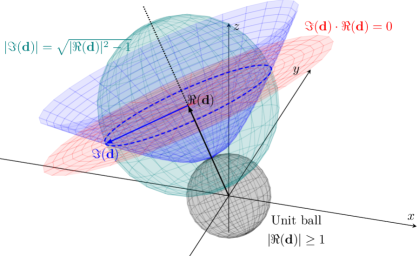
Figure 2.1: Geometrical representation of the constraints in (2.1). The black dotted line (which originates on the boundary of the unit ball) and the blue hyperboloid depict respectively the real and imaginary parts of elements in the set $\{\mathbf{d}=R_{\bm{\theta},\psi}\,\mathbf{d}_{\uparrow}\left(1+\zeta/2\kappa\right),(\psi,\zeta)\in[0,2\pi)\times[0,+\infty)\}$ for fixed $\bm{\theta}\in\Theta$, see (2.3).

We start by introducing and studying evanescent plane waves (EPWs) in 3D. These waves satisfy the Helmholtz equation (1.1) and generalize the well-known propagative plane waves (PPWs) while preserving their simple exponential form. This section also presents the modal analysis tools that are later used to analyse approximation properties of both types of plane waves. In particular, we extend the classical Jacobi–Anger expansion to complex propagation directions, and use this to compute the coefficients of the spherical-wave expansion of any EPW.

2.1 Definition

A plane wave $\mathbf{x}\mapsto e^{i\kappa\mathbf{d}\cdot\mathbf{x}}$ satisfies the homogeneous Helmholtz equation (1.1) if and only if the direction vector $\mathbf{d}=(\textup{d}_{1},\textup{d}_{2},\textup{d}_{3})\in\mathbb{C}^{3}$ fulfills the constraint $\mathbf{d}\cdot\mathbf{d}=\sum_{i=1}^{3}\textup{d}_{i}^{2}=1$, or equivalently

$$\left|\Re\left(\mathbf{d}\right)\right|^{2}-\left|\Im\left(\mathbf{d}\right)\right|^{2}=1,\quad\text{(a)}\qquad\qquad\qquad\Re\left(\mathbf{d}\right)\cdot\Im\left(\mathbf{d}\right)=0.\quad\text{(b)}$$ (2.1)

Hence, $\Re\left(\mathbf{d}\right)$ is required only to have a modulus larger than $1$, and $\Im\left(\mathbf{d}\right)$ must lie on the circle of radius of $(\left|\Re\left(\mathbf{d}\right)\right|^{2}-1)^{1/2}$ in the plane orthogonal to $\Re\left(\mathbf{d}\right)$, see Figure 2.1. We parametrize the set $\{\mathbf{d}\in\mathbb{C}^{3}:\mathbf{d}\cdot\mathbf{d}=1\}$ by fixing a reference complex direction vector $\mathbf{d}_{\uparrow}$ that meets conditions (2.1), and then considering all its possible rigid-body rotations in space. For instance, if we let $\Re\left(\mathbf{d}_{\uparrow}\right)$ be aligned with the $z$-axis, we can pick $\Im\left(\mathbf{d}_{\uparrow}\right)$ aligned with the $x$-axis so that (2.1b) is satisfied, and then (2.1a) simplifies to $\Re\left(\textup{d}_{\uparrow,3}\right)^{2}-\Im\left(\textup{d}_{\uparrow,1}\right)^{2}=1$. Assuming $\textup{d}_{\uparrow,1}\geq 0$ and $\textup{d}_{\uparrow,3}\geq 0$, and setting $z:=\Re\left(\textup{d}_{\uparrow,3}\right)\geq 1$, we get $\Im\left(\textup{d}_{\uparrow,1}\right)=(z^{2}-1)^{1/2}$. This prompts us to propose the following definition and parametrization of an evanescent plane wave.

Definition 2.1 (Evanescent plane wave).

Let $\bm{\theta}:=(\theta_{1},\theta_{2})\in\Theta:=[0,\pi]\times[0,2\pi)$, $\psi\in[0,2\pi)$ be the Euler angles and $R_{\bm{\theta},\psi}:=R_{z}(\theta_{2})R_{y}(\theta_{1})R_{z}(\psi)$ the associated rotation matrix, where

$$R_{y}(\theta):=\begin{bmatrix}\cos{(\theta)}&0&\sin{(\theta)}\\ 0&1&0\\ -\sin{(\theta)}&0&\cos{(\theta)}\end{bmatrix},\qquad R_{z}(\theta):=\begin{bmatrix}\cos{(\theta)}&-\sin{(\theta)}&0\\ \sin{(\theta)}&\cos{(\theta)}&0\\ 0&0&1\end{bmatrix}.$$

For any $\mathbf{y}:=(\bm{\theta},\psi,\zeta)\in Y:=\Theta\times[0,2\pi)\times[0,+\infty)$, we let

$$\textup{EW}_{\mathbf{y}}(\mathbf{x}):=e^{i\kappa\mathbf{d}(\mathbf{y})\cdot\mathbf{x}}\qquad\forall\mathbf{x}\in\mathbb{R}^{3},$$ (2.2)

where the wave complex direction is given by

$$\mathbf{d}(\mathbf{y}):=R_{\bm{\theta},\psi}\,\mathbf{d}_{\uparrow}\left(1+\zeta/2\kappa\right)\in\mathbb{C}^{3},\qquad\text{and}\qquad\mathbf{d}_{\uparrow}(z):=\left(i\sqrt{z^{2}-1},0,z\right)\in\mathbb{C}^{3}\quad\forall z\geq 1.$$ (2.3)

Remark 2.2.

We parametrize $\mathbf{d}(\mathbf{y})$ in (2.3) with three angles $\theta_{1},\theta_{2},\psi$ and with $\zeta\geq 0$, while $\mathbf{d}_{\uparrow}$ is parametrized by $z\geq 1$, related to $\zeta$ by $z=1+\zeta/2\kappa$. This choice, although not immediately apparent, leads to simpler results in the subsequent analysis.

Assuming $\zeta=0$ in (2.2), for any $(\bm{\theta},\psi)\in\Theta\times[0,2\pi)$, we recover the standard definition of a propagative plane wave. For any $\bm{\theta}\in\Theta$, we let

$$\textup{PW}_{\bm{\theta}}(\mathbf{x}):=\textup{EW}_{(\bm{\theta},0,0)}(\mathbf{x})=e^{i\kappa\mathbf{d}(\bm{\theta})\cdot\mathbf{x}}\qquad\forall\mathbf{x}\in\mathbb{R}^{3},$$ (2.4)

where the wave propagation direction is given by

$$\mathbf{d}(\bm{\theta}):=\left(\sin\theta_{1}\cos\theta_{2},\>\sin\theta_{1}\sin\theta_{2},\>\cos\theta_{1}\right)\in\mathbb{S}^{2}:=\{\mathbf{x}\in\mathbb{R}^{3}:|\mathbf{x}|=1\}\subset\mathbb{R}^{3}.$$ (2.5)

Here, $\mathbf{d}(\bm{\theta})$ does not depend on $\psi$, as $\mathbf{d}_{\uparrow}(1)=(0,0,1)$ is invariant under the rotation $R_{z}(\psi)$.

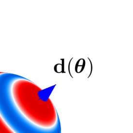
(a) ​​​​​​​​​​​​​$\psi=\cdot\,$, $\zeta=0$

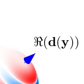
(b) ​​​​​​​​​​​​​$\psi=\pi$, $\zeta=2$

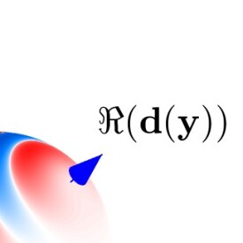
(c) ​​​​​​​​​​​​​$\psi=0$, $\zeta=2$

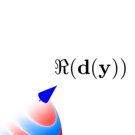
(d) ​​​​​​​​​​​$\psi=\pi$, $\zeta=20$

Figure 2.2: Real part of some EPWs in (2.2) restricted to $\partial B_{1}$. The blue arrow denotes $\Re\left(\mathbf{d}(\mathbf{y})\right)$ direction, i.e. $\mathbf{d}(\bm{\theta})$ in (2.5), while the red arrow represents $\Im\left(\mathbf{d}(\mathbf{y})\right)$ direction, i.e. $\mathbf{d}^{\bot}(\bm{\theta},\psi)$, that is the first column of the rotation matrix $R_{\bm{\theta},\psi}$. We set $\theta_{1}=\theta_{2}=\pi/4$ and wavenumber $\kappa=16$.

Since the direction vector $\mathbf{d}(\mathbf{y})$ in (2.3) is complex valued, the wave behavior can become unclear. A more explicit expression of the EPW (2.2) is

$$\textup{EW}_{\mathbf{y}}(\mathbf{x})=e^{i\kappa\Re(\mathbf{d}(\mathbf{y}))\cdot\mathbf{x}}e^{-\kappa\Im(\mathbf{d}(\mathbf{y}))\cdot\mathbf{x}}=e^{i\left(\frac{\zeta}{2}+\kappa\right)\mathbf{d}(\bm{\theta})\cdot\mathbf{x}}e^{-\left(\zeta\left(\frac{\zeta}{4}+\kappa\right)\right)^{1/2}\mathbf{d}^{\bot}(\bm{\theta},\psi)\cdot\mathbf{x}},$$ (2.6)

where $\mathbf{d}(\bm{\theta})$ is defined in (2.5) and we denote with $\mathbf{d}^{\bot}(\bm{\theta},\psi)$ the first column of the matrix $R_{\bm{\theta},\psi}$. The wave oscillates with apparent wavenumber $\zeta/2+\kappa\geq\kappa$ in the propagation direction $\mathbf{d}(\bm{\theta})$, parallel to $\Re\left(\mathbf{d}(\mathbf{y})\right)$. Additionally, the wave decays exponentially in the direction $\mathbf{d}^{\bot}(\bm{\theta},\psi)$, which is orthogonal to $\mathbf{d}(\bm{\theta})$ and parallel to $\Im\left(\mathbf{d}(\mathbf{y})\right)$. This justifies naming the new parameters $(\psi,\zeta)\in[0,2\pi)\times[0,+\infty)$, which control the imaginary part of the complex direction $\mathbf{d}(\mathbf{y})$ in (2.3), evanescence parameters. Some EPWs are represented in Figure 2.2.

2.2 Spherical waves

For spherical domains, an explicit orthonormal basis for the Helmholtz solution space is given by acoustic Fourier modes, the so-called spherical waves. To define them, we briefly review some special functions.

For conciseness, we introduce the index set $\mathcal{I}:=\{(\ell,m)\in\mathbb{Z}^{2}:0\leq|m|\leq\ell\}$. Following [19, eqs. (14.7.10) and (14.9.3)], the Ferrers functions are defined, for all $(\ell,m)\in\mathcal{I}$ and $|x|\leq 1$, as

$$\mathsf{P}_{\ell}^{m}(x):=\frac{(-1)^{m}}{2^{\ell}\ell!}(1-x^{2})^{\frac{m}{2}}\frac{\textup{d}^{\ell+m}}{\textup{d}x^{\ell+m}}(x^{2}-1)^{\ell},\!\!\qquad\!\!\text{so that}\!\!\qquad\!\!\mathsf{P}_{\ell}^{-m}(x)=(-1)^{m}\frac{(\ell-m)!}{(\ell+m)!}\mathsf{P}_{\ell}^{m}(x).$$ (2.7)

In particular, $\mathsf{P}_{\ell}:=\mathsf{P}_{\ell}^{0}$ are simply called Legendre polynomials of degree $\ell$. Following [19, eq. (14.30.1)], for every $(\theta,\varphi)\in\Theta$ and $(\ell,m)\in\mathcal{I}$, the spherical harmonics are defined as

$$Y_{\ell}^{m}(\theta,\varphi):=\gamma_{\ell}^{m}e^{im\varphi}\mathsf{P}_{\ell}^{m}(\cos{\theta}),\qquad\text{where}\qquad\gamma_{\ell}^{m}:=\left[\frac{2\ell+1}{4\pi}\frac{(\ell-m)!}{(\ell+m)!}\right]^{1/2}$$ (2.8)

is a normalization constant, such that $\|Y_{\ell}^{m}\|_{L^{2}(\mathbb{S}^{2})}=1$. With a little abuse of notation, we also write $Y_{\ell}^{m}(\mathbf{x})$ in place of $Y_{\ell}^{m}(\theta,\varphi)$, for $\mathbf{x}=(\sin\theta\cos\varphi,\sin\theta\sin\varphi,\cos\theta)\in\mathbb{S}^{2}$. These functions constitute an orthonormal basis of $L^{2}(\mathbb{S}^{2})$. The Condon–Shortley convention is used, i.e. the phase factor of $(-1)^{m}$ is included in (2.7) rather than in $\gamma_{\ell}^{m}$. Finally, for every $r>0$, we denote with $j_{\ell}(r):=\sqrt{\pi/2r}J_{\ell+1/2}(r)$ the spherical Bessel functions [19, eq. (10.47.3)], where $J_{\ell}(r)$ are the usual Bessel functions [19, eq. (10.2.2)].

We are now ready to define the spherical waves. For normalization purposes, let us introduce the following $\kappa$-dependent Hermitian product and associated norm:

$$(u,v)_{\mathcal{B}}:=(u,v)_{L^{2}(B_{1})}+\kappa^{-2}(\nabla u,\nabla v)_{L^{2}(B_{1})^{3}},\qquad\|u\|^{2}_{\mathcal{B}}:=(u,u)_{\mathcal{B}}\qquad\forall u,v\in H^{1}(B_{1}).$$ (2.9)

(a) Propagative: $\ell=2m=\kappa/2=8$

(b) Grazing: $\ell=2m=\kappa=16$

(c) Evanescent: $\ell=2m=3\kappa=48$

Figure 2.3: Real part of some spherical waves $b_{\ell}^{m}$ on $\partial\{B_{1}\setminus\{\mathbf{x}\in\mathbb{R}^{3}:\mathbf{x}>0\}\}$. With increasing order $\ell$, these functions concentrates progressively closer to the boundary $\partial B_{1}$.

Definition 2.3 (Spherical waves).

We define, for any $(\ell,m)\in\mathcal{I}$

$$b_{\ell}^{m}:=\beta_{\ell}\tilde{b}_{\ell}^{m},\qquad\text{where}\qquad\tilde{b}_{\ell}^{m}(\mathbf{x}):=j_{\ell}(\kappa|\mathbf{x}|)Y_{\ell}^{m}(\mathbf{x}/|\mathbf{x}|)\quad\forall\mathbf{x}\in B_{1},\qquad\beta_{\ell}:=\|\tilde{b}_{\ell}^{m}\|^{-1}_{\mathcal{B}}.$$ (2.10)

Furthermore, we introduce the space $\mathcal{B}:=\overline{\textup{span}\{b_{\ell}^{m}\}_{(\ell,m)\in\mathcal{I}}}^{\|\cdot\|_{\mathcal{B}}}\subsetneq H^{1}(B_{1})$.

Thanks to [18, eq. (2.4.23)] and [19, eq. (10.47.1)] it is clear that the spherical waves satisfy the Helmholtz equation (1.1). Although $b_{\ell}^{m}$ depends on the two indices $(\ell,m)\in\mathcal{I}$, the normalization factor $\beta_{\ell}$ is independent of $m$, as shown later in Lemma 2.5.

Following common terminology, we refer to spherical waves with mode number $\ell<\kappa$ (resp. $\ell\gg\kappa$) as propagative (resp. evanescent) modes; their ‘energy’ is distributed throughout the unit ball (resp. concentrated near the unit sphere). Lastly, waves with $\ell\approx\kappa$ are called grazing modes. Figure 2.3 illustrates the behavior of several functions $b_{\ell}^{m}$ on the boundary of the unit ball without the first octant. Below, we report the results obtained in [10, Lem. 1.2 and 1.3].

Lemma 2.4.

The space $(\mathcal{B},\!\|\cdot\|_{\mathcal{B}})$ is a Hilbert space and the family $\{b_{\ell}^{m}\}_{(\ell,m)\in\mathcal{I}}$ is a Hilbert basis:

$$(b_{\ell}^{m},b_{q}^{n})_{\mathcal{B}}=\delta_{\ell,q}\delta_{m,n}\quad\forall(\ell,m),(q,n)\in\mathcal{I},\qquad\text{and}\qquad u=\sum_{(\ell,m)\in\mathcal{I}}(u,b_{\ell}^{m})_{\mathcal{B}}\,b_{\ell}^{m}\quad\forall u\in\mathcal{B}.$$

Moreover, $u\in H^{1}(B_{1})$ satisfies the Helmholtz equation (1.1) if and only if $u\in\mathcal{B}$.

The upcoming analysis uses the asymptotics of the normalization coefficient $\beta_{\ell}$, which grows super-exponentially with $\ell$ after a pre-asymptotic regime up to $\ell\approx\kappa$.

Lemma 2.5.

We have for all $\ell\geq 0$

$$\beta_{\ell}=\sqrt{\frac{2\kappa}{\pi}}\left[(1+{\ell}/{\kappa^{2}})J^{2}_{\ell+\frac{1}{2}}(\kappa)-(J_{\ell-\frac{1}{2}}(\kappa)+J_{\ell+\frac{1}{2}}(\kappa)/\kappa)J_{\ell+\frac{3}{2}}(\kappa)\right]^{-\frac{1}{2}}\underset{\ell\rightarrow\infty}{\sim}2^{\frac{3}{2}}\kappa\left(\frac{2}{e\kappa}\right)^{\ell}\ell^{\ell+\frac{1}{2}}.$$ (2.11)

Proof.

Since $b_{\ell}^{m}$ solves the Helmholtz equation (1.1), the expansion in (2.11) stems from

$$\beta_{\ell}^{-2}=\|\tilde{b}_{\ell}^{m}\|^{2}_{\mathcal{B}}=2\|\tilde{b}_{\ell}^{m}\|^{2}_{L^{2}(B_{1})}+\kappa^{-2}(\partial_{\mathbf{n}}\tilde{b}_{\ell}^{m},\tilde{b}_{\ell}^{m})_{L^{2}(\partial B_{1})},$$ (2.12)

and, using [19, eqs. (10.22.5) and (10.51.2)],

$$\|\tilde{b}_{\ell}^{m}\|^{2}_{L^{2}(B_{1})}=\int_{0}^{1}\!\!j^{2}_{\ell}(\kappa r)r^{2}\textup{d}r=\frac{\pi}{2\kappa}\int_{0}^{1}\!\!J^{2}_{\ell+\frac{1}{2}}(\kappa r)r\textup{d}r=\frac{\pi}{4\kappa}\left(J^{2}_{\ell+\frac{1}{2}}(\kappa)-J_{\ell-\frac{1}{2}}(\kappa)J_{\ell+\frac{3}{2}}(\kappa)\right),$$ (2.13)

$$(\partial_{\mathbf{n}}\tilde{b}_{\ell}^{m},\tilde{b}_{\ell}^{m})_{L^{2}(\partial B_{1})}=\kappa j^{\prime}_{\ell}(\kappa)j_{\ell}(\kappa)=\ell j^{2}_{\ell}(\kappa)-\kappa j_{\ell}(\kappa)j_{\ell+1}(\kappa)=\frac{\pi}{2\kappa}\left(\ell J^{2}_{\ell+\frac{1}{2}}(\kappa)-\kappa J_{\ell+\frac{1}{2}}(\kappa)J_{\ell+\frac{3}{2}}(\kappa)\right).$$ (2.14)

The proof of the asymptotic behavior consists in showing that we have as $\ell\rightarrow\infty$

$$\|\tilde{b}_{\ell}^{m}\|^{2}_{L^{2}(B_{1})}\sim\frac{1}{16}\left(\frac{e\kappa}{2}\right)^{2\ell}\ell^{-2\left(\ell+\frac{3}{2}\right)},\qquad\text{and}\qquad(\partial_{\mathbf{n}}\tilde{b}_{\ell}^{m},\tilde{b}_{\ell}^{m})_{L^{2}(\partial B_{1})}\sim\frac{1}{8}\left(\frac{e\kappa}{2}\right)^{2\ell}\ell^{-2\left(\ell+\frac{1}{2}\right)}.$$

Hence, thanks to (2.12), the dominant term in $\|\tilde{b}_{\ell}^{m}\|_{\mathcal{B}}$ in the limit $\ell\rightarrow\infty$ is the boundary one.

Let us consider the $L^{2}(B_{1})$ norm. From (2.13) and since [19, eq. (10.19.1)] holds, namely

$$J_{\ell}(r)\sim\frac{1}{\sqrt{2\pi\ell}}\left(\frac{er}{2\ell}\right)^{\ell}\qquad\text{as}\,\,\,\ell\rightarrow\infty,$$ (2.15)

we get as $\ell\rightarrow\infty$

$$\|\tilde{b}_{\ell}^{m}\|^{2}_{L^{2}(B_{1})}\sim\frac{1}{8\kappa}\left(\frac{e\kappa}{2}\right)^{2\ell+1}\left(\ell+\frac{1}{2}\right)^{-2(\ell+1)}\Bigg{[}1-\frac{\left(\ell+\frac{1}{2}\right)^{2(\ell+1)}}{\left(\ell-\frac{1}{2}\right)^{\ell}\left(\ell+\frac{3}{2}\right)^{\ell+2}}\Bigg{]}.$$ (2.16)

Moreover, since for every $x,y,z\in\mathbb{R}$

$$(\ell+x)^{y\ell+z}\sim\ell^{y\ell+z}\exp\bigg{\{}{xy+\frac{x(2z-xy)}{2\ell}}\bigg{\}}\sim\ell^{y\ell+z}e^{xy}\qquad\text{as}\,\,\,\ell\rightarrow\infty,$$ (2.17)

the term inside the square brackets in (2.16) is equivalent to $\ell^{-1}$ at infinity.

Consider now the term $(\partial_{\mathbf{n}}\tilde{b}_{\ell}^{m},\tilde{b}_{\ell}^{m})_{L^{2}(\partial B_{1})}$ in (2.12). From (2.14) and (2.15), we get as $\ell\rightarrow\infty$

$$(\partial_{\mathbf{n}}\tilde{b}_{\ell}^{m},\tilde{b}_{\ell}^{m})_{L^{2}(\partial B_{1})}\sim\frac{1}{4\kappa}\left(\frac{e\kappa}{2}\right)^{2\ell+1}\left(\ell+\frac{1}{2}\right)^{-2(\ell+1)}\left[\ell-\frac{e\kappa^{2}}{2}\frac{\left(\ell+\frac{1}{2}\right)^{\ell+1}}{\left(\ell+\frac{3}{2}\right)^{\ell+2}}\right],$$

and, thanks to (2.17), it is readily checked that the second term inside the square brackets is dominated by the first one, since it is equivalent to $\kappa^{2}/2\ell$ at infinity. ∎

2.3 Complex-direction Jacobi–Anger identity

The explicit series expansion of PPWs in the spherical wave basis is given by the Jacobi–Anger identity [17, eq. (14)], namely

$$\textup{PW}_{\bm{\theta}}(\mathbf{x})=4\pi\sum_{\ell=0}^{\infty}i^{\ell}\sum_{m=-\ell}^{\ell}\overline{Y_{\ell}^{m}\left(\bm{\theta}\right)}j_{\ell}(\kappa|\mathbf{x}|)Y_{\ell}^{m}(\mathbf{x}/|\mathbf{x}|)\qquad\forall\mathbf{x}\in B_{1},\,\forall\bm{\theta}\in\Theta.$$ (2.18)

The goal of this section is to obtain a similar expansion for EPWs, i.e. for complex-valued directions $\mathbf{d}(\mathbf{y})$, which to the best of our knowledge is not available in the literature. This generalization is not trivial and requires additional definitions and lemmas.

Associated Legendre functions

Following [8, sect. 3.2, eq. (6)], we adopt the convention

$$(w^{2}-1)^{m/2}:=\mathcal{P}\left[(w+1)^{m/2}\right]\,\mathcal{P}\left[(w-1)^{m/2}\right]\qquad\forall m\in\mathbb{Z},\,\forall w\in\mathbb{C},$$ (2.19)

where $\mathcal{P}[\,\,\cdot\,\,]$ indicates the standard principal branch. For odd $m$, (2.19) allows to eliminate the branch cut along the imaginary axis simply by mirroring the function values from the right-half of the complex plane to the left-half (see [10, sect. 4.2]). Following [19, eqs. (14.7.14) and (14.9.13)], the associated Legendre functions are defined, for every $(\ell,m)\in\mathcal{I}$ and $w\in\mathbb{C}$, as

$$P_{\ell}^{m}(w):=\frac{1}{2^{\ell}\ell!}(w^{2}-1)^{\frac{m}{2}}\frac{\textup{d}^{\ell+m}}{\textup{d}w^{\ell+m}}(w^{2}-1)^{\ell},\!\!\qquad\!\!\text{so that}\!\!\qquad\!\!P_{\ell}^{-m}(w)=\frac{(\ell-m)!}{(\ell+m)!}P_{\ell}^{m}(w).$$ (2.20)

For every odd $m$, $P_{\ell}^{m}$ is a single-valued function on the complex plane with a branch cut along the interval $(-1,1)$, where it is continuous from above; otherwise, if $m$ is even, $P_{\ell}^{m}$ is a polynomial of degree $\ell$. Notably, $P_{\ell}(w):=P_{\ell}^{0}(w)=\mathsf{P}_{\ell}(w)$ for all $w\in\mathbb{C}$. From [19, eq. (14.23.1)], it follows:

$$\lim_{\epsilon\searrow 0}P_{\ell}^{m}(x\pm i\epsilon)=(\pm 1)^{m}P_{\ell}^{m}(x)=i^{\mp m}\mathsf{P}_{\ell}^{m}(x)\qquad\forall x\in(-1,1).$$ (2.21)

The next lemma extends the identity [7, eq. (2.46)] to complex values of $t$:

$$e^{irt}=\sum_{\ell=0}^{\infty}i^{\ell}(2\ell+1)j_{\ell}(r)\mathsf{P}_{\ell}(t)\qquad\forall r\geq 0,\,\forall t\in[-1,1].$$ (2.22)

Lemma 2.6.

Let $\ell\geq 0$. We have for every $0\leq m\leq\ell$ and $w\in\mathbb{C}$

$$P_{\ell}^{m}(w)=\frac{(\ell+m)!}{2^{\ell}\ell!}\sum_{k=0}^{\ell-m}\binom{\ell}{k}\binom{\ell}{m+k}\left(w-1\right)^{\ell-\left(m/2+k\right)}\left(w+1\right)^{m/2+k}.$$ (2.23)

In particular, due to (2.20), $P_{\ell}^{m}(z)\geq 0$ for every real $z\geq 1$ and $(\ell,m)\in\mathcal{I}$. Moreover,

$$e^{irw}=\sum_{\ell=0}^{\infty}i^{\ell}(2\ell+1)j_{\ell}(r)P_{\ell}(w)\qquad\forall r\geq 0,\,\forall w\in\mathbb{C}.$$ (2.24)

Proof.

It can be readily seen that

$$\frac{\textup{d}^{\ell+m}}{\textup{d}w^{\ell+m}}(w^{2}-1)^{\ell} =\sum_{k=0}^{\ell+m}\binom{\ell+m}{k}\left(\frac{\textup{d}^{k}}{\textup{d}w^{k}}(w-1)^{\ell}\right)\left(\frac{\textup{d}^{\ell+m-k}}{\textup{d}w^{\ell+m-k}}(w+1)^{\ell}\right)$$

$$=\sum_{k=m}^{\ell}\binom{\ell+m}{k}\left(\frac{\ell!}{(\ell-k)!}(w-1)^{\ell-k}\right)\left(\frac{\ell!}{(k-m)!}(w+1)^{k-m}\right)$$

$$=\frac{(w-1)^{\ell}}{(w+1)^{m}}\sum_{k=m}^{\ell}\frac{(\ell+m)!}{k!(\ell+m-k)!}\frac{\ell!}{(\ell-k)!}\frac{\ell!}{(k-m)!}\left(\frac{w+1}{w-1}\right)^{k}$$

$$=(\ell+m)!(w-1)^{\ell-m}\sum_{k=0}^{\ell-m}\binom{\ell}{k}\binom{\ell}{m+k}\left(\frac{w+1}{w-1}\right)^{k}.$$

Therefore, thanks to the definitions (2.19) and (2.20), the expansion (2.23) follows.

Let $R>1$ and $B_{R}:=\{w\in\mathbb{C}:|w|<R\}$. We want to check that the right-hand side in (2.24) is well-defined for every $r\geq 0$ and $w\in B_{R}$. Due to (2.15) and (2.17), it is enough to prove

$$\sum_{\ell=0}^{\infty}\left(\frac{er}{2\ell+1}\right)^{\ell}\left|P_{\ell}(w)\right|<\infty\qquad\forall r\geq 0,\,\forall w\in B_{R}.$$ (2.25)

Thanks to (2.23), $P_{\ell}=P_{\ell}^{0}$, and the Vandermonde identity [25, eq. (1)], it follows

$$|P_{\ell}(w)|\leq\frac{1}{2^{\ell}}\sum_{k=0}^{\ell}\binom{\ell}{k}^{2}|w-1|^{\ell-k}|w+1|^{k}\leq\sum_{k=0}^{\ell}\binom{\ell}{k}^{2}\left(\frac{R+1}{2}\right)^{\ell}=\binom{2\ell}{\ell}\left(\frac{R+1}{2}\right)^{\ell},$$

and therefore, for every $r\geq 0$ and $w\in B_{R}$, the series (2.25) is dominated by

$$\sum_{\ell=0}^{\infty}c_{\ell},\qquad\text{where}\qquad c_{\ell}:=\binom{2\ell}{\ell}\left[\frac{er(R+1)}{4\ell+2}\right]^{\ell}.$$ (2.26)

The series (2.26) is convergent, as confirmed by the ratio test: in fact, from (2.17), we have

$$\frac{c_{\ell+1}}{c_{\ell}}\sim\left(\frac{\ell+1/2}{\ell+3/2}\right)^{\ell+1}\frac{er(R+1)}{\ell+1}\sim\frac{r(R+1)}{\ell}\qquad\text{as }\ell\rightarrow\infty.$$

Thus, the right-hand side of (2.24) is well-defined for every $r\geq 0$ and $w\in B_{R}$. The functions $w\mapsto e^{irw}$ and $w\mapsto P_{\ell}(w)$ are analytic on $B_{R}$ and, since identity (2.22) holds, that is (2.24) with $w\in[-1,1]$, it follows that (2.24) also holds for every $r\geq 0$ and $w\in B_{R}$ due to [1, Th. 3.2.6]. As $R>1$ is arbitrary, (2.24) is valid for every $w\in\mathbb{C}$. ∎

Wigner matrices, rotations of spherical harmonics and addition theorem

The next definition aligns with [22, eq. (34)] and [9, eq. (1)], albeit with a distinction: we invert the angle signs to ensure consistency with the notation of PPW directions in (2.5).

Definition 2.7 (Wigner matrices).

Let $(\bm{\theta},\psi)\in\Theta\times[0,2\pi)$ be the Euler angles and $\ell\geq 0$. The Wigner D-matrix is the unitary matrix $D_{\ell}(\bm{\theta},\psi)=(D_{\ell}^{m,m^{\prime}}\!(\bm{\theta},\psi))_{m,m^{\prime}}\!\in\mathbb{C}^{(2\ell+1)\times(2\ell+1)}$, where

$$D_{\ell}^{m,m^{\prime}}(\bm{\theta},\psi):=e^{im^{\prime}\theta_{2}}d_{\ell}^{\,m,m^{\prime}}(\theta_{1})e^{im\psi}\qquad\forall\,|m|,|m^{\prime}|\leq\ell.$$ (2.27)

In turn, $d_{\ell}(\theta):=(d_{\ell}^{\,m,m^{\prime}}\!(\theta))_{m,m^{\prime}}\!\in\mathbb{R}^{(2\ell+1)\times(2\ell+1)}$ is called Wigner d-matrix and its entries are:

$$d_{\ell}^{\,m,m^{\prime}}(\theta):=\sum_{k=k_{\textup{min}}}^{k_{\textup{max}}}w_{\ell,k}^{m,m^{\prime}}\left(\cos{\frac{\theta}{2}}\right)^{2(\ell-k)+m^{\prime}-m}\left(\sin{\frac{\theta}{2}}\right)^{2k+m-m^{\prime}}\qquad\forall\,|m|,|m^{\prime}|\leq\ell,$$ (2.28)

where

$$w_{\ell,k}^{m,m^{\prime}}:=\frac{(-1)^{k}\left[(\ell+m)!(\ell-m)!(\ell+m^{\prime})!(\ell-m^{\prime})!\right]^{1/2}}{(\ell-m-k)!(\ell+m^{\prime}-k)!(k+m-m^{\prime})!\,k!},$$

with $k_{\textup{min}}:=\max\{0,m^{\prime}-m\}$ and $k_{\textup{max}}:=\max\{\ell-m,\ell+m^{\prime}\}$.

The Wigner D-matrix $D_{\ell}(\bm{\theta},\psi)$ is used to express the image of any spherical harmonic of degree $\ell$ under the rotation $R_{\bm{\theta},\psi}$ as a linear combination of spherical harmonics of the same degree. In fact the expansion formula [26, sect. 4.1, eq. (5)] holds, namely

$$Y_{\ell}^{m}(\mathbf{x})=\sum_{m^{\prime}=-\ell}^{\ell}\overline{D_{\ell}^{m,m^{\prime}}(\bm{\theta},\psi)}Y_{\ell}^{m^{\prime}}(R_{\bm{\theta},\psi}\mathbf{x})\qquad\forall\mathbf{x}\in\mathbb{S}^{2},\,\forall(\ell,m)\in\mathcal{I}.$$ (2.29)

We finally establish a generalized Legendre addition theorem, extending e.g. [7, eq. (2.30)].

Lemma 2.8.

For any $\ell\geq 0$, $\mathbf{x}\in\mathbb{S}^{2}$ and $\mathbf{y}=(\bm{\theta},\psi,\zeta)\in Y$ we have

$$\sum_{{m}=-\ell}^{\ell}\sum_{{m^{\prime}}=-\ell}^{\ell}\overline{D_{\ell}^{m^{\prime},m}(\bm{\theta},\psi)}\gamma_{\ell}^{m^{\prime}}i^{-m^{\prime}}P_{\ell}^{m^{\prime}}\left(1+{\zeta}/{2\kappa}\right)Y_{\ell}^{m}(\mathbf{x})=\frac{2\ell+1}{4\pi}P_{\ell}(\mathbf{d}(\mathbf{y})\cdot\mathbf{x}),$$ (2.30)

Proof.

Let $\mathbf{x}=(\sin{\theta}\cos{\varphi},\sin{\theta}\sin{\varphi},\cos{\theta})\in\mathbb{S}^{2}$ with $(\theta,\varphi)\in\Theta$ and let $\mathbf{y}=(\bm{\theta},\psi,\zeta)\in Y$ with $z=1+\zeta/2\kappa$. We need to establish that

$$\sum_{m=-\ell}^{\ell}\gamma_{\ell}^{m}i^{-m}P_{\ell}^{m}(z)Y_{\ell}^{m}(\mathbf{x})=\frac{2\ell+1}{4\pi}P_{\ell}(\mathbf{d}_{\uparrow}(z)\cdot\mathbf{x}),$$ (2.31)

from which the result follows using (2.29) and $\mathbf{d}(\mathbf{y})=R_{\bm{\theta},\psi}\mathbf{d_{\uparrow}}(z)$ from (2.3). On the one hand,

$$P_{\ell}\left(z\cos\theta+i\sqrt{z^{2}-1}\sin\theta\cos\varphi\right)=P_{\ell}\left(\mathbf{d}_{\uparrow}(z)\cdot\mathbf{x}\right).$$

On the other hand, thanks to (2.7), (2.8), and (2.20),

$$\frac{4\pi}{2\ell+1}\!\sum_{m=-\ell}^{\ell}(\gamma_{\ell}^{m})^{2}i^{-m}P_{\ell}^{m}(z)\mathsf{P}_{\ell}^{m}(\cos\theta)e^{im\varphi}=\!\!\sum_{m=-\ell}^{\ell}\frac{(\ell-m)!}{(\ell+m)!}i^{-m}P_{\ell}^{m}(z)\mathsf{P}_{\ell}^{m}(\cos\theta)e^{im\varphi}$$

$$=\sum_{m=0}^{\ell}\frac{(\ell-m)!}{(\ell+m)!}i^{-m}P_{\ell}^{m}(z)\mathsf{P}_{\ell}^{m}(\cos\theta)e^{im\varphi}+\sum_{m=1}^{\ell}\frac{(\ell-m)!}{(\ell+m)!}i^{-m}P_{\ell}^{m}(z)\mathsf{P}_{\ell}^{m}(\cos\theta)e^{-im\varphi}$$

$$=P_{\ell}(z)\mathsf{P}_{\ell}(\cos\theta)+2\sum_{m=1}^{\ell}\frac{(\ell-m)!}{(\ell+m)!}i^{-m}P_{\ell}^{m}(z)\mathsf{P}_{\ell}^{m}(\cos\theta)\cos(m\varphi).$$

From (2.21) and the branch cut convention (2.19) we get

$$\lim_{\epsilon\searrow 0} \bigg{[}P_{\ell}(z)P_{\ell}(\cos\theta-i\epsilon)+2\sum_{m=1}^{\ell}\frac{(\ell-m)!}{(\ell+m)!}(-1)^{m}P_{\ell}^{m}(z)P_{\ell}^{m}(\cos\theta-i\epsilon)\cos(m\varphi)\bigg{]}$$

$$=P_{\ell}(z)\mathsf{P}_{\ell}(\cos\theta)+2\sum_{m=1}^{\ell}\frac{(\ell-m)!}{(\ell+m)!}i^{-m}P_{\ell}^{m}(z)\mathsf{P}_{\ell}^{m}(\cos\theta)\cos(m\varphi),\,\,\,$$

$$\lim_{\epsilon\searrow 0} \bigg{[}P_{\ell}\left(z(\cos\theta-i\epsilon)-\sqrt{z^{2}-1}\sqrt{(\cos\theta-i\epsilon)^{2}-1}\cos\varphi\right)\bigg{]}\!=\!P_{\ell}\left(z\cos\theta+i\sqrt{z^{2}-1}\sin\theta\cos\varphi\right).$$

Due to [19, eqs. (14.7.16) and (14.28.1)], the arguments of the two limits coincide. Thanks to the previous computations made in this proof, the equality of the limits leads to (2.31). ∎

Remark 2.9.

To clarify, [19, eq. (14.28.1)] only states that the equality between the limit arguments holds when $\theta\in[0,\pi/2)$. Consequently, identities (2.30) are established solely in this case. The limitation likely arises because [19] does not adopt the convention (2.19) in the definition of the associated Legendre functions. Thus, [19, eq. (14.28.1)] is applicable only to values with positive real part. Nevertheless, since all terms in (2.30) are analytic in $(0,\pi)$ as functions of $\theta$ (making explicit the dependence of $\mathbf{x}$ on $\theta$), these identities can be easily extended to this interval due to [1, Th. 3.2.6]. Furthermore, they hold if $\mathbf{x}=(0,0,1)$, namely $\theta=\pi$: in fact $\mathsf{P}_{\ell}^{m}(-1)=(-1)^{\ell}\delta_{0,m}$ and, due to [19, eq. (14.7.17)], $P_{\ell}(-z)=(-1)^{\ell}P_{\ell}(z)$ for every $z\geq 1$.

Generalized Jacobi–Anger identity

Theorem 2.10.

EPWs admit the following modal expansion: for any $\mathbf{x}\in B_{1}$, $\mathbf{y}=(\bm{\theta},\psi,\zeta)\in Y$,

$$\textup{EW}_{\mathbf{y}}(\mathbf{x})=4\pi\sum_{\ell=0}^{\infty}i^{\ell}\!\!\sum_{{m}=-\ell}^{\ell}\left[\sum_{{m^{\prime}}=-\ell}^{\ell}\overline{D_{\ell}^{m^{\prime},m}(\bm{\theta},\psi)}\gamma_{\ell}^{m^{\prime}}i^{-m^{\prime}}P_{\ell}^{m^{\prime}}\!\!\left(1+\frac{\zeta}{2\kappa}\right)\right]j_{\ell}(\kappa|\mathbf{x}|)Y_{\ell}^{m}(\mathbf{x}/|\mathbf{x}|).$$ (2.32)

Proof.

The result follows from applying (2.30) after using (2.24) to obtain

$$\textup{EW}_{\mathbf{y}}(\mathbf{x}):=e^{i\kappa\mathbf{d}(\mathbf{y})\cdot\mathbf{x}}=\sum_{\ell=0}^{\infty}i^{\ell}(2\ell+1)j_{\ell}(\kappa|\mathbf{x}|)P_{\ell}\big{(}\mathbf{d}(\mathbf{y})\cdot\mathbf{x}/|\mathbf{x}|\big{)}\qquad\forall\mathbf{x}\in B_{1},\ \forall\mathbf{y}\in Y.\qed$$

Remark 2.11.

Thanks to (2.27), [22, eq. (35)] and the Wigner d-matrix symmetry properties [26, sect. 4.4, eq. (1)], it holds

$$D_{\ell}^{0,m}(\bm{\theta},\psi)=\sqrt{\frac{(\ell-m)!}{(\ell+m)!}}\,e^{im\theta_{2}}\mathsf{P}_{\ell}^{m}(\cos\theta_{1})\qquad\forall(\bm{\theta},\psi)\in\Theta\times[0,2\pi),\,\forall(\ell,m)\in\mathcal{I},$$ (2.33)

and moreover $P_{\ell}^{m}(1)=\delta_{0,m}$ due to (2.20). Hence, assuming $\zeta=0$ in (2.32), we recover the Jacobi–Anger expansion (2.18) for PPWs for any $(\bm{\theta},\psi)\in\Theta\times[0,2\pi)$.

2.4 Modal analysis of plane waves

The Jacobi–Anger identity (2.32) plays a crucial role in the upcoming analysis. As we develop below, this modal expansion with respect to the $b_{\ell}^{m}$ basis also offers direct insights on the approximation properties of EPWs, hinting at why such waves are better suited for approximating less regular Helmholtz solutions compared to PPWs.

$\widehat{\textup{EW}}_{\ell}^{m}\!\!\left(\frac{\pi}{4},\cdot,0\right)$	$\widehat{\textup{EW}}_{\ell}^{m}\!\!\left(\frac{\pi}{4},\frac{\pi}{2},60\right)$	$\widehat{\textup{EW}}_{\ell}^{m}\!\!\left(\frac{\pi}{4},\frac{3\pi}{2},60\right)$	$\widehat{\textup{EW}}_{\ell}^{m}\!\!\left(\frac{\pi}{4},\frac{\pi}{4},120\right)$	$\widehat{\textup{EW}}_{\ell}^{m}\!\!\left(\frac{\pi}{4},\frac{7\pi}{4},120\right)$	$\widehat{\textup{EW}}_{\ell}^{m}\!\!\left(\frac{\pi}{4},0,180\right)$

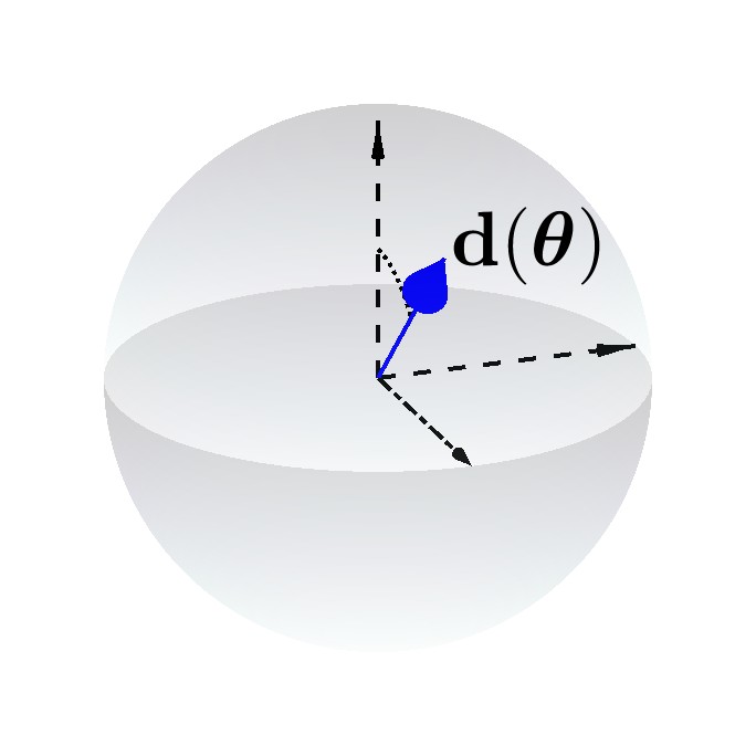
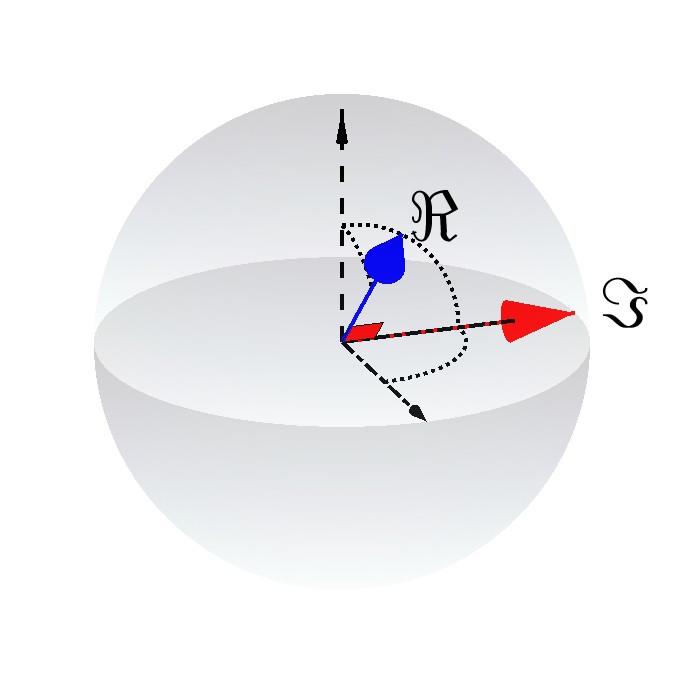
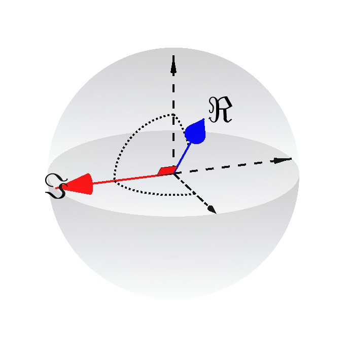
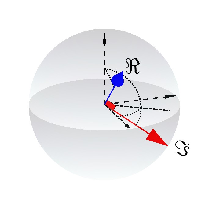
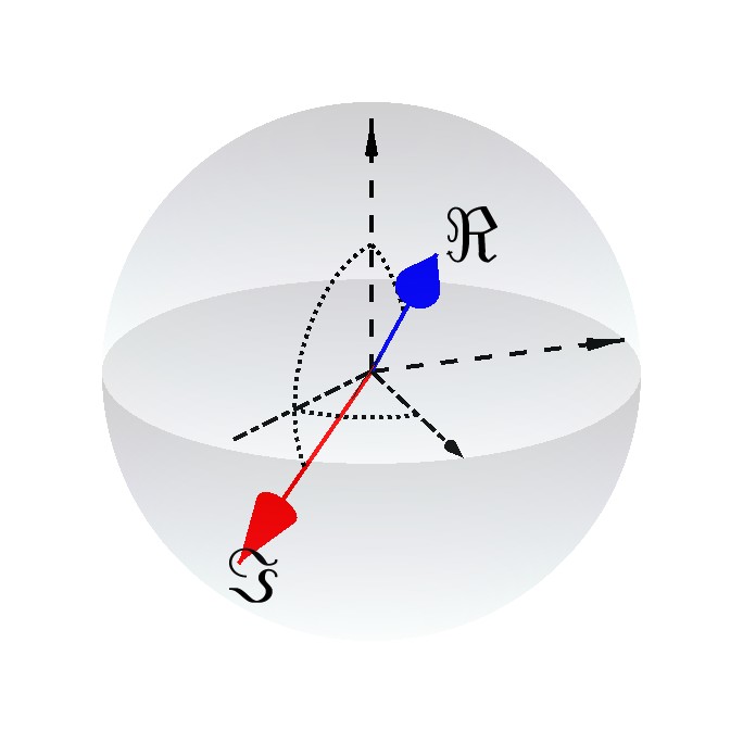
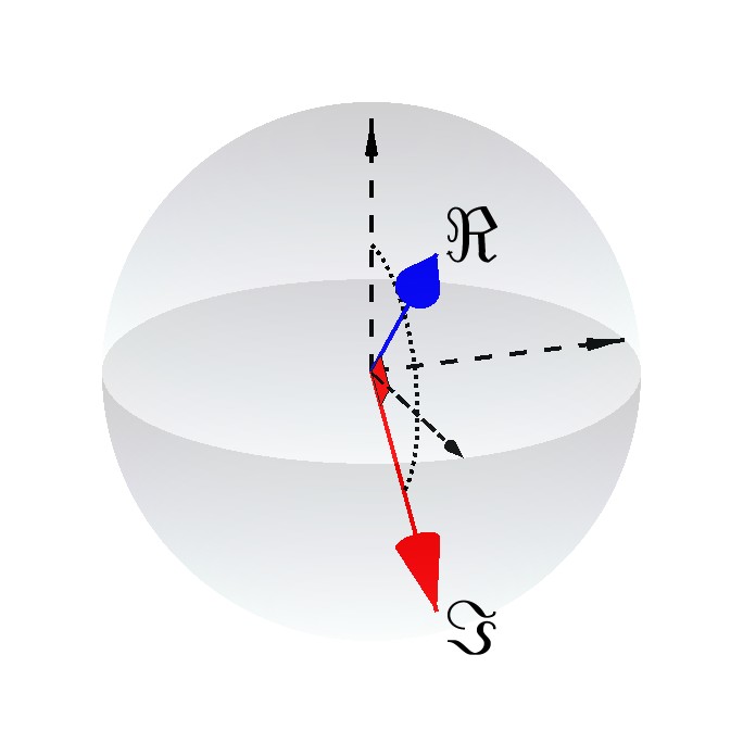
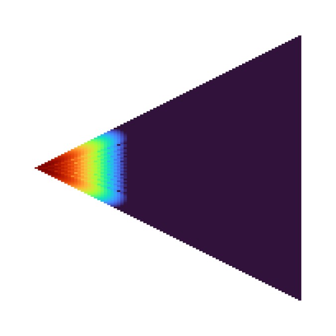
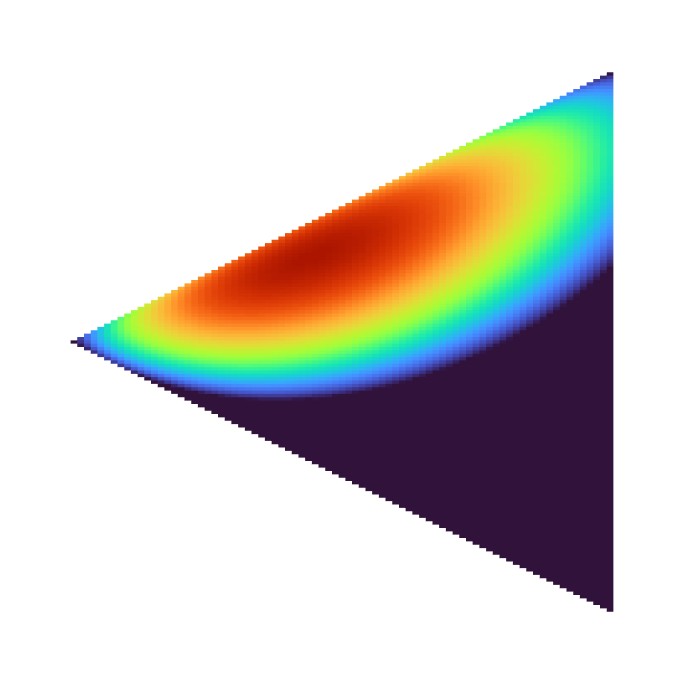
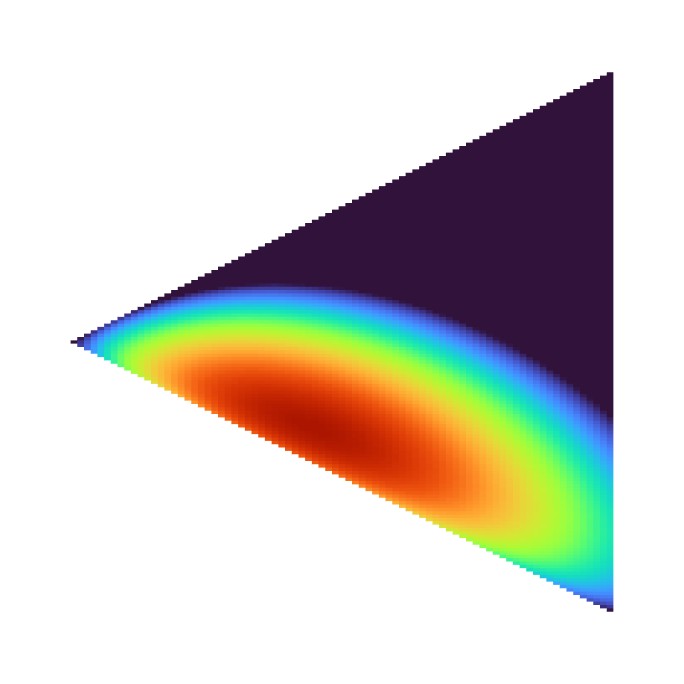
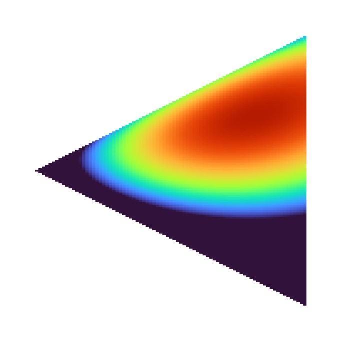
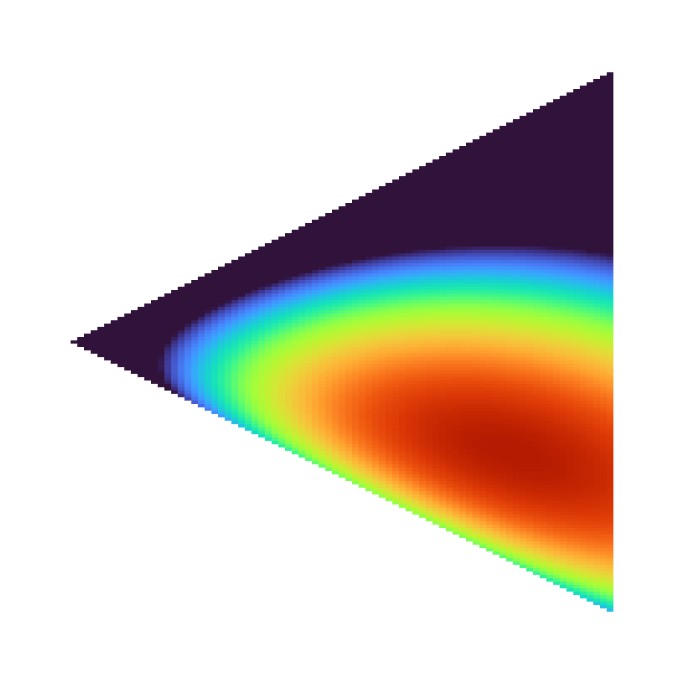
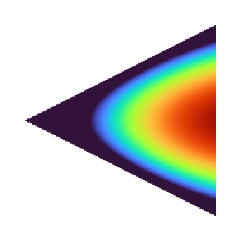
Figure 2.4: Modal analysis of EPWs. For each wave: (top) representations of both real and imaginary components of direction vectors $\mathbf{d}(\mathbf{y})$ with fixed angle $\theta_{2}=0$; (bottom) related distributions of the coefficients $\widehat{\textup{EW}}_{\ell}^{m}\!(\theta_{1},\psi,\zeta)$ in (2.36). To mitigate the numerical cancellation issue of Wigner’s formula (2.28), we rely on [9] using [10, eq. (4.26)]. The index $\ell$ varies on the abscissa within the range $0\leq\ell\leq 80$, while the index $m$ varies on the ordinate within the range $0\leq|m|\leq\ell$, forming a triangle. The coefficients have been suitably normalized using a normalization factor described in the subsequent sections, see (5.6), which depends solely on $\zeta$. Wavenumber $\kappa=6$. More plots of this kind can be seen in [10, sect. 4.4].

For conciseness, we use the notation $\mathbf{D}^{m}_{\ell}(\bm{\theta},\psi)$, for $0\leq|m|\leq\ell$, to represent the columns of the Wigner D-matrix $D_{\ell}(\bm{\theta},\psi)$ in (2.27) and we let

$$\mathbf{P}_{\ell}(\zeta):=\big{(}\gamma_{\ell}^{m}i^{m}P_{\ell}^{m}(1+\zeta/2\kappa)\big{)}_{m=-\ell}^{\ell}\in\mathbb{C}^{2\ell+1}\qquad\forall\ell\geq 0.$$ (2.34)

Recalling (2.10), the Jacobi–Anger expansion (2.32) can be written as

$$\textup{EW}_{\mathbf{y}}(\mathbf{x})=\sum_{\ell=0}^{\infty}\sum_{{m}=-\ell}^{\ell}\left[4\pi i^{\ell}\beta_{\ell}^{-1}\overline{\mathbf{D}^{m}_{\ell}(\bm{\theta},\psi)\cdot\mathbf{P}_{\ell}(\zeta)}\right]b_{\ell}^{m}(\mathbf{x})\qquad\forall\mathbf{x}\in B_{1},\forall\mathbf{y}\in Y.$$ (2.35)

The moduli of the coefficients in the above modal expansion, namely

$$\widehat{\textup{EW}}_{\ell}^{m}\!(\theta_{1},\psi,\zeta)\!:=\!\left|\left(\textup{EW}_{\mathbf{y}},b_{\ell}^{m}\right)_{\mathcal{B}}\right|\!=\!\frac{4\pi}{\beta_{\ell}}\left|\sum_{m^{\prime}=-\ell}^{\ell}\!\!\gamma_{\ell}^{m^{\prime}}i^{-m^{\prime}}\!d_{\ell}^{\,m^{\prime},m}(\theta_{1})e^{-im^{\prime}\psi}P_{\ell}^{m^{\prime}}\!\!\left(1+\frac{\zeta}{2\kappa}\right)\right|,$$ (2.36)

are depicted in Figure 2.4. We also define, for any $\ell\geq 0$ and $\mathbf{y}=(\bm{\theta},\psi,\zeta)\in Y$,

$$b_{\ell}[\mathbf{y}]:=\widehat{\textup{EW}}_{\ell}^{-1}(\zeta)\,\tilde{b}_{\ell}[\mathbf{y}],\quad\text{where}\quad\tilde{b}_{\ell}[\mathbf{y}]:=\sum_{m=-\ell}^{\ell}\left(\textup{EW}_{\mathbf{y}},b_{\ell}^{m}\right)_{\mathcal{B}}b_{\ell}^{m},\quad\widehat{\textup{EW}}_{\ell}(\zeta):=\big{\|}\tilde{b}_{\ell}[\mathbf{y}]\big{\|}_{\mathcal{B}}.$$ (2.37)

In fact, thanks to (2.37), we can expand the EPWs as

$$\textup{EW}_{\mathbf{y}}=\sum_{\ell=0}^{\infty}\sum_{m=-\ell}^{\ell}\left(\textup{EW}_{\mathbf{y}},b_{\ell}^{m}\right)_{\mathcal{B}}b_{\ell}^{m}=\sum_{\ell=0}^{\infty}\tilde{b}_{\ell}[\mathbf{y}]=\sum_{\ell=0}^{\infty}\widehat{\textup{EW}}_{\ell}(\zeta)\,b_{\ell}[\mathbf{y}],$$

where $b_{\ell}[\mathbf{y}]\in\text{span}\{b_{\ell}^{m}\}_{m=-\ell}^{\ell}$ are orthonormal and

$$\widehat{\textup{EW}}_{\ell}(\zeta)=\,\left(\sum_{m=-\ell}^{\ell}\left|\left(\textup{EW}_{\mathbf{y}},b_{\ell}^{m}\right)_{\mathcal{B}}\right|^{2}\right)^{1/2}=\left(\sum_{m=-\ell}^{\ell}\left[\widehat{\textup{EW}}_{\ell}^{m}\!(\theta_{1},\psi,\zeta)\right]^{2}\right)^{1/2}=\,\frac{4\pi}{\beta_{\ell}}\left|\mathbf{P}_{\ell}(\zeta)\right|.$$ (2.38)

The last equality in (2.38) holds due to (2.36) and the unitarity condition [26, sect. 4.1, eq. (6)]. Figure 2.5 shows the coefficient distribution (2.38) for various values of $\zeta$.

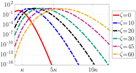
Figure 2.5: Modal analysis of EPWs: distributions of the coefficients (2.38) for various values of the evanescence parameter $\zeta$. For each $\zeta$, this involves computing the $\ell^{2}$-norms along the vertical segments of the coefficient distribution triangles, such as those in Figure 2.4. As $\zeta$ increases, higher-$\ell$ Fourier modes can be encompassed, transitioning away from the propagative case represented by $\zeta=0$. The coefficients have been suitably normalized using a normalization factor described in the subsequent sections, see (5.6). Wavenumber $\kappa=6$.

Remark 2.12.

Assuming $\zeta=0$, the functions $b_{\ell}\left[\mathbf{y}\right]$ coincide, up to the multiplicative constant $i^{\ell}$, with the spherical waves $b_{\ell}^{0}$ rotated according to the PPW angles $\bm{\theta}\in\Theta$. This is readily checked thanks to (2.8) and (2.10), along with the identities (2.29) and (2.33).

If we consider PPWs and thus assume $\zeta=0$, the coefficients (2.36) are independent of $\psi$. For any $\bm{\theta}\in\Theta$, the PPW coefficients decay super-exponentially fast in the evanescent-mode regime $\ell\gg\kappa$. This is visible in the leftmost triangle of Figure 2.4 and in the continuous line in Figure 2.5. Consequently, any PPW approximation of Helmholtz solutions with a high-$\ell$ Fourier modal content will require exponentially large coefficients and cancellation to capture these modes, resulting in numerical instability. This assertion is made precise later in Lemma 3.13 and Lemma 4.4.

On the contrary, by tuning the evanescence parameters $\psi$ and $\zeta$, the Fourier modal content of the EPWs can be shifted to higher Fourier regimes. Specifically, raising $\zeta$ enables us to reach higher degrees (larger values of $\ell$), while varying $\psi$ allows us to cover different orders $m$. As a consequence we expect EPWs with large $\zeta$ to be able to approximate high Fourier modes with relatively small coefficients, curing the numerical instability experienced with PPWs. However, accurately selecting the evanescence parameters $\psi$ and $\zeta$ to build reasonably sized approximation spaces remains a significant challenge. We will tackle this issue in the following sections.

3 Stable continuous approximation

PPWs and EPWs families are naturally indexed by continuous sets, the parametric domains $\Theta$ and $Y$ in Definition 2.1. Although in applications a finite discrete subset is selected, it is fruitful to first analyse the properties of the continuous set of plane waves. This is the purpose of this section which first introduces the notion of stable continuous approximation. We then present the Herglotz density space, showing its close link with the Helmholtz solution space through the Jacobi–Anger identity (2.35). This connection leads to the definition of the Herglotz transform, an integral operator enabling the representation of any Helmholtz solution in the unit ball as a continuous superposition of EPWs. This continuous representation is proven to be stable, as opposed to PPWs, which fail to produce such a result due to their inability to stably represent evanescent spherical modes, i.e. solutions dominated by high-order Fourier modes.

3.1 The concept of stable continuous approximation

Let $(X,\mu)$ be a $\sigma$-finite measure space and denote by $L^{2}_{\mu}(X)$ the corresponding Lebesgue space. Following [5, sect. 5.6], we define a Bessel family in the Hilbert space $\mathcal{B}$ as a set

$$\mathbf{\Phi}_{X}:=\{\phi_{x}\}_{x\in X}\subset\mathcal{B},\qquad\text{such that}\qquad\int_{X}|\left(u,\phi_{x}\right)_{\mathcal{B}}|^{2}\textup{d}\mu(x)\leq B\|u\|^{2}_{\mathcal{B}}\qquad\forall u\in\mathcal{B},$$

for some $B>0$. For any such $\mathbf{\Phi}_{X}$, the synthesis operator can be defined as:

$$\bm{\mathrm{T}}_{\!X}^{\scaleto{\textup{\,}\mathstrut}{5pt}}:L_{\mu}^{2}(X)\rightarrow\mathcal{B},\quad v\mapsto\int_{X}v(x)\phi_{x}\textup{d}\mu(x).$$

Definition 3.1 (Stable continuous approximation).

The Bessel family $\mathbf{\Phi}_{X}$ is said to be a stable continuous approximation for $\mathcal{B}$ if, for any tolerance $\eta>0$, there exists a stability constant $C_{\textup{cs}}\geq 0$ such that

$$\forall u\in\mathcal{B},\ \exists v\in L_{\mu}^{2}(X):\quad\left\|u-\bm{\mathrm{T}}_{\!X}^{\scaleto{\textup{\,}\mathstrut}{5pt}}v\right\|_{\mathcal{B}}\leq\eta\|u\|_{\mathcal{B}},\quad\text{and}\quad\|v\|_{L^{2}_{\mu}(X)}\leq C_{\textup{cs}}\|u\|_{\mathcal{B}}.$$ (3.1)

A stable continuous approximation allows approximating any Helmholtz solution to a given accuracy as an expansion $\bm{\mathrm{T}}_{\!X}^{\scaleto{\textup{\,}\mathstrut}{5pt}}v$, where the density $v$ has a bounded norm in $L_{\mu}^{2}(X)$.

3.2 Herglotz density space

We consider the space $L_{\nu}^{2}(Y)$ on the EPW parametric domain $Y$, with the positive measure $\nu$ given by

$$\textup{d}\nu(\mathbf{y}):=\textup{d}\sigma(\bm{\theta})\,\textup{d}\psi\,w(\zeta)\textup{d}\zeta,\qquad\text{where}\qquad w(\zeta):=\zeta^{1/2}e^{-\zeta}\quad\forall\zeta\in[0,+\infty),$$ (3.2)

and $\sigma$ is the standard measure on $\mathbb{S}^{2}$. The $L_{\nu}^{2}$ Hermitian product and the associated norm are

$$(v,u)_{\mathcal{A}}:=\int_{Y}v(\mathbf{y})\overline{u(\mathbf{y})}\textup{d}\nu(\mathbf{y}),\qquad\|v\|^{2}_{\mathcal{A}}:=(v,v)_{\mathcal{A}}\qquad\qquad\forall v,u\in L_{\nu}^{2}(Y).$$

Let us define a proper subspace of $L_{\nu}^{2}(Y)$, denoted by $\mathcal{A}$ and named space of Herglotz densities.

Definition 3.2 (Herglotz densities).

We define, for any $(\ell,m)\in\mathcal{I}$

$$a_{\ell}^{m}:=\alpha_{\ell}\tilde{a}_{\ell}^{m},\quad\text{where}\quad\tilde{a}_{\ell}^{m}(\mathbf{y}):=\mathbf{D}^{m}_{\ell}(\bm{\theta},\psi)\cdot\mathbf{P}_{\ell}(\zeta)\quad\forall\mathbf{y}=(\bm{\theta},\psi,\zeta)\in Y,\quad\alpha_{\ell}:=\|\tilde{a}_{\ell}^{m}\|^{-1}_{\mathcal{A}},$$ (3.3)

where $\mathbf{D}^{m}_{\ell}(\bm{\theta},\psi)$ and $\mathbf{P}_{\ell}(\zeta)$ are defined in (2.34), and $\mathcal{A}:=\overline{\textup{span}\{a_{\ell}^{m}\}_{(\ell,m)\in\mathcal{I}}}^{\|\cdot\|_{\mathcal{A}}}\subsetneq L_{\nu}^{2}(Y)$.

Just like the spherical waves (2.10), the Herglotz densities also depend on $(\ell,m)\in\mathcal{I}$, while the normalization coefficient $\alpha_{\ell}$ is independent of $m$, as will be clarified later (see Lemma 3.6). The wavenumber $\kappa$ appears explicitly in the definition (2.34) of $\mathbf{P}_{\ell}(\zeta)$, hence each $a_{\ell}^{m}$ depends on it. Several plots of the functions $a_{\ell}^{m}$ can be seen in [10, Fig. 5.1].

Lemma 3.3.

​The space $(\mathcal{A},\!\|\cdot\|_{\mathcal{A}})$ is a Hilbert space and the family $\{a_{\ell}^{m}\}_{\!(\ell,m)\in\mathcal{I}}$ is a Hilbert basis:

$$(a_{\ell}^{m},a_{q}^{n})_{\mathcal{A}}=\delta_{\ell,q}\delta_{m,n}\quad\forall(\ell,m),(q,n)\in\mathcal{I},\qquad\text{and}\qquad v=\sum_{(\ell,m)\in\mathcal{I}}(v,a_{\ell}^{m})_{\mathcal{A}}\,a_{\ell}^{m}\quad\forall v\in\mathcal{A}.$$

Using Definition 3.2, the Jacobi–Anger expansion (2.35) takes the simple form

$$\textup{EW}_{\mathbf{y}}(\mathbf{x})=\sum_{(\ell,m)\in\mathcal{I}}\tau_{\ell}\,\overline{a_{\ell}^{m}(\mathbf{y})}\,b_{\ell}^{m}(\mathbf{x}),\qquad\text{where}\qquad\tau_{\ell}:=4\pi i^{\ell}(\alpha_{\ell}\beta_{\ell})^{-1}\qquad\forall\ell\geq 0.$$ (3.4)

The formula (3.4) holds a crucial role as it establishes a link between the spherical wave basis (2.10) of the space $\mathcal{B}$ and the Herglotz-density basis (3.3) of the space $\mathcal{A}$ through EPWs in (2.2).

The behavior of $\tau_{\ell}$ for large $\ell$ will intervene in the upcoming analysis. To study this, we start with a lemma useful to analyze the asymptotic behavior of the normalization coefficients $\alpha_{\ell}$.

Lemma 3.4.

We have for all $(\ell,m)\in\mathcal{I}$ and $z\geq 1$

$$(z-1)^{\ell}\leq\frac{\sqrt{\pi}(\ell-m)!P_{\ell}^{m}(z)}{2^{\ell}\Gamma\left(\ell+1/2\right)}\leq(z+1)^{\ell}.$$ (3.5)

Proof.

Due to (2.20), $(\ell+m)!P_{\ell}^{-m}(z)=(\ell-m)!P_{\ell}^{m}(z)$ for every $(\ell,m)\in\mathcal{I}$, allowing us to assume $m\geq 0$ from here on. Thanks to (2.23) and [19, eq. (5.5.5)], it readily follows:

$$A_{\ell}^{m}(z):=\frac{\sqrt{\pi}(\ell-m)!P_{\ell}^{m}(z)}{2^{\ell}\Gamma\left(\ell+1/2\right)}=\binom{2\ell}{\ell+m}^{-1}\left(z-1\right)^{\ell}\sum_{k=0}^{\ell-m}\binom{\ell}{k}\binom{\ell}{m+k}\left(\frac{z+1}{z-1}\right)^{m/2+k}.$$

Thanks to the Vandermonde identity [25, eq. (1)] and $\binom{a}{b}=\binom{a}{a-b}$, we derive:

$$A_{\ell}^{m}(z) \leq\binom{2\ell}{\ell+m}^{-1}\!\left(\frac{z+1}{z-1}\right)^{\ell-m/2}\!\!\!(z-1)^{\ell}\sum_{k=0}^{\ell-m}\binom{\ell}{k}\binom{\ell}{m+k}=\left(\frac{z-1}{z+1}\right)^{m/2}\!\!\!(z+1)^{\ell}\leq(z+1)^{\ell},$$

$$A_{\ell}^{m}(z) \geq\binom{2\ell}{\ell+m}^{-1}(z-1)^{\ell}\sum_{k=0}^{\ell-m}\binom{\ell}{k}\binom{\ell}{m+k}=(z-1)^{\ell}.\qed$$

Remark 3.5.

Numerical evidence suggests that a sharper upper bound in (3.5) is $z^{\ell}$.

After a pre-asymptotic regime up to $\ell\approx\kappa$, the coefficients $\alpha_{\ell}$ exhibit super-exponential decay with respect to $\ell$. The specific asymptotic behavior is detailed in the next lemma.

Lemma 3.6.

For a constant $c(\kappa)$ only depending on $\kappa$, we have

$$\alpha_{\ell}\sim c(\kappa)\left(\frac{e\kappa}{2}\right)^{\ell}\ell^{-\left(\ell+\frac{1}{2}\right)}\qquad\text{as}\ \ell\rightarrow\infty.$$ (3.6)

Proof.

We have that

$$\|\tilde{a}_{\ell}^{m}\|^{2}_{\mathcal{A}} =\int_{Y}|\mathbf{D}^{m}_{\ell}(\bm{\theta},\psi)\cdot\mathbf{P}_{\ell}(\zeta)|^{2}\textup{d}\nu(\mathbf{y})$$

$$=\sum_{m^{\prime}=-\ell}^{\ell}\int_{\Theta}\int_{0}^{2\pi}\left|D_{\ell}^{m^{\prime},m}(\bm{\theta},\psi)\right|^{2}\textup{d}\sigma(\bm{\theta})\textup{d}\psi\int_{0}^{+\infty}\left[\gamma_{\ell}^{m^{\prime}}P_{\ell}^{m^{\prime}}\left(1+\zeta/2\kappa\right)\right]^{2}w(\zeta)\textup{d}\zeta$$

$$=\frac{8\pi^{2}}{2\ell+1}\sum_{m^{\prime}=-\ell}^{\ell}\int_{0}^{+\infty}\left[\gamma_{\ell}^{m^{\prime}}P_{\ell}^{m^{\prime}}\left(1+\zeta/2\kappa\right)\right]^{2}\zeta^{1/2}e^{-\zeta}\textup{d}\zeta.$$ (3.7)

In what follows, we study the integral in (3.7), henceforth denoted by $B_{\ell}^{m^{\prime}}$. Thanks to (3.5):

$$B_{\ell}^{m^{\prime}} \geq\left(\frac{2^{\ell}\gamma_{\ell}^{m^{\prime}}\Gamma(\ell+1/2)}{\sqrt{\pi}(\ell-m^{\prime})!}\right)^{2}\int_{0}^{+\infty}\left(\frac{\zeta}{2\kappa}\right)^{2\ell}\zeta^{1/2}e^{-\zeta}\textup{d}\zeta$$

$$=\frac{1}{4\pi^{2}\kappa^{2\ell}}\frac{(2\ell+1)\Gamma^{\,2}(\ell+1/2)}{(\ell+m^{\prime})!(\ell-m^{\prime})!}\,\Gamma\left(2\ell+\frac{3}{2}\right)=:C_{\ell}^{m^{\prime}},$$ (3.8)

and analogously

$$B_{\ell}^{m^{\prime}} \leq\left(\frac{2^{\ell}\gamma_{\ell}^{m^{\prime}}\Gamma(\ell+1/2)}{\sqrt{\pi}(\ell-m^{\prime})!}\right)^{2}\int_{0}^{+\infty}\left(\frac{\zeta}{2\kappa}+2\right)^{2\ell}\zeta^{1/2}e^{-\zeta}\textup{d}\zeta$$

$$=\left(\frac{2^{\ell}\gamma_{\ell}^{m^{\prime}}\Gamma(\ell+1/2)}{\sqrt{\pi}(\ell-m^{\prime})!}\right)^{2}\int_{4\kappa}^{+\infty}\left(\frac{\eta}{2\kappa}\right)^{2\ell}(\eta-4\kappa)^{1/2}e^{-(\eta-4\kappa)}\textup{d}\eta$$

$$<\frac{2\ell+1}{4\pi^{2}}\frac{2^{2\ell}\Gamma^{\,2}(\ell+1/2)}{(\ell+m^{\prime})!(\ell-m^{\prime})!}\int_{0}^{+\infty}\left(\frac{\eta}{2\kappa}\right)^{2\ell}\eta^{1/2}e^{-\eta}e^{4\kappa}\textup{d}\eta$$

$$=\frac{e^{4\kappa}}{4\pi^{2}\kappa^{2\ell}}\frac{(2\ell+1)\Gamma^{\,2}(\ell+1/2)}{(\ell+m^{\prime})!(\ell-m^{\prime})!}\,\Gamma\left(2\ell+\frac{3}{2}\right)=e^{4\kappa}C_{\ell}^{m^{\prime}},$$ (3.9)

where $\eta=\zeta+4\kappa$. Using (2.17) and [19, eq. (5.11.3)], it is easily checked that as $\ell\rightarrow+\infty$

$$\Gamma\left(2\ell+3/2\right) \sim\sqrt{2\pi}e^{-\left(2\ell+3/2\right)}\left(2\ell+3/2\right)^{2\ell+1}\sim\sqrt{2\pi}e^{-2\ell}\left(2\ell\right)^{2\ell+1},$$

$$\Gamma^{\,2}\left(\ell+1/2\right) \sim 2\pi e^{-(2\ell+1)}\left(\ell+1/2\right)^{2\ell}\sim 2\pi e^{-2\ell}\ell^{2\ell},$$

$$(\ell+m^{\prime})!(\ell-m^{\prime})! \sim 2\pi e^{-2(\ell+1)}(\ell+m^{\prime}+1)^{\ell+m^{\prime}+1/2}(\ell-m^{\prime}+1)^{\ell-m^{\prime}+1/2}\sim 2\pi e^{-2\ell}\ell^{2\ell+1},$$

where $|m^{\prime}|\leq\ell$ is fixed, and hence

$$\frac{(2\ell+1)\Gamma^{\,2}(\ell+1/2)}{(\ell+m^{\prime})!(\ell-m^{\prime})!}\Gamma\left(2\ell+\frac{3}{2}\right)\sim 2\sqrt{2\pi}e^{-2\ell}(2\ell)^{2\ell+1}\qquad\text{as }\ell\rightarrow+\infty.$$

By combining (3.8) and (3.9), it follows that, as $\ell\rightarrow+\infty$, there exists a constant $c_{1}(\kappa)$, only dependent on the wavenumber $\kappa$, such that

$$C_{\ell}^{m^{\prime}}\sim\frac{\sqrt{2}}{\pi\sqrt{\pi}}\left(\frac{2}{e\kappa}\right)^{2\ell}\ell^{2\ell+1}\qquad\Rightarrow\qquad B_{\ell}^{m^{\prime}}\sim c_{1}(\kappa)\left(\frac{2}{e\kappa}\right)^{2\ell}\ell^{2\ell+1}.$$

Moreover, also $\|\tilde{a}_{\ell}^{m}\|^{2}_{\mathcal{A}}$ has the same behavior as $B_{\ell}^{m^{\prime}}$ at infinity: in fact, thanks to (3.7), we have

$$\|\tilde{a}_{\ell}^{m}\|^{2}_{\mathcal{A}} \sim\frac{4\pi^{2}}{\ell}\sum_{m^{\prime}=-\ell}^{\ell}c_{1}(\kappa)\left(\frac{2}{e\kappa}\right)^{2\ell}\ell^{2\ell+1}\sim c_{2}(\kappa)\left(\frac{2}{e\kappa}\right)^{2\ell}\ell^{2\ell+1},$$

for some constant $c_{2}(\kappa)$ only dependent on $\kappa$; the claimed result (3.6) follows from (3.3). ∎

From the asymptotics provided in Lemma 2.5 and Lemma 3.6, we can deduce the next result.

Corollary 3.7.

The coefficients $\tau_{\ell}$ in (3.4) are uniformly bounded in $\ell$, namely

$$\tau_{-}:=\inf_{\ell\geq 0}|\tau_{\ell}|>0\qquad\text{and}\qquad\tau_{+}:=\sup_{\ell\geq 0}|\tau_{\ell}|<\infty.$$ (3.10)

Figure 3.1: Dependence of $|\tau_{\ell}|$ on the mode number $\ell$ for various wavenumber $\kappa$.

Figure 3.2: Dependence of $\tau_{\pm}$ defined in (3.10) on the wavenumber $\kappa$.

The behavior of $|\tau_{\ell}|$ is shown in Figure 3.1 for different wavenumbers $\kappa$. This plot aligns with the results in (3.10), displaying a flat asymptotic behavior for larger values of $\ell$. Moreover, the values $\tau_{\pm}$ depend on the wavenumber $\kappa$, as shown in Figure 3.2.

3.3 Herglotz integral representation

Introducing the Herglotz transform $\bm{\mathrm{T}}_{Y}^{\scaleto{\textup{EW}\mathstrut}{5pt}}$, we can represent any Helmholtz solution in $\mathcal{B}$ as a linear combination of EPWs, each weighted by an element of $\mathcal{A}$. This integral operator is well-defined on $\mathcal{A}$ thanks to the following result.

Lemma 3.8.

$\{\textup{EW}_{\mathbf{y}}\}_{\mathbf{y}\in Y}$ is a Bessel family for $\mathcal{B}$, where the optimal Bessel bound is $B=\tau_{+}^{2}$.

Proof.

This can be seen directly from Lemma 3.3 and the Jacobi–Anger identity (3.4):

$$\int_{Y}|(u,\textup{EW}_{\mathbf{y}})_{\mathcal{B}}|^{2}\textup{d}\nu(\mathbf{y})=\sum_{(\ell,m)\in\mathcal{I}}|\tau_{\ell}|^{2}|(u,b_{\ell}^{m})_{\mathcal{B}}|^{2}\leq\tau_{+}^{2}\|u\|^{2}_{\mathcal{B}}\qquad\forall u\in\mathcal{B}.\qed$$

The synthesis operator $\bm{\mathrm{T}}_{Y}^{\scaleto{\textup{EW}\mathstrut}{5pt}}$ associated to the EPW family is defined, for any $v\in L_{\nu}^{2}(Y)$, by

$$\boxed{\left(\bm{\mathrm{T}}_{Y}^{\scaleto{\textup{EW}\mathstrut}{5pt}}v\right)(\mathbf{x}):=\int_{Y}v(\mathbf{y})\textup{EW}_{\mathbf{y}}(\mathbf{x})\textup{d}\nu(\mathbf{y})\qquad\forall\mathbf{x}\in B_{1}.}$$ (3.11)

The following theorem, extension to 3D of [20, Th. 6.7], shows that for any Helmholtz solution $u\in\mathcal{B}$ there exists a unique corresponding Herglotz density $v\in\mathcal{A}$ such that $u=\bm{\mathrm{T}}_{Y}^{\scaleto{\textup{EW}\mathstrut}{5pt}}v$ and justifies the use of the term ‘transform’ associated to $\bm{\mathrm{T}}_{Y}^{\scaleto{\textup{EW}\mathstrut}{5pt}}$.

Theorem 3.9.

The operator $\bm{\mathrm{T}}_{Y}^{\scaleto{\textup{EW}\mathstrut}{5pt}}$ is bounded and invertible from $\mathcal{A}$ to $\mathcal{B}$:

$$\bm{\mathrm{T}}_{Y}^{\scaleto{\textup{EW}\mathstrut}{5pt}}\!:\mathcal{A}\rightarrow\mathcal{B},\;\;v\mapsto\!\!\!\!\!\sum_{(\ell,m)\in\mathcal{I}}\!\!\!\tau_{\ell}(v,a_{\ell}^{m})_{\mathcal{A}}b_{\ell}^{m},\quad\text{and}\quad\tau_{-}\|v\|_{\mathcal{A}}\leq\left\|\bm{\mathrm{T}}_{Y}^{\scaleto{\textup{EW}\mathstrut}{5pt}}v\right\|_{\mathcal{B}}\leq\tau_{+}\|v\|_{\mathcal{A}}\;\;\forall v\in\mathcal{A}.$$ (3.12)

In particular, $\bm{\mathrm{T}}_{Y}^{\scaleto{\textup{EW}\mathstrut}{5pt}}$ is diagonal on the space bases, namely $\bm{\mathrm{T}}_{Y}^{\scaleto{\textup{EW}\mathstrut}{5pt}}a_{\ell}^{m}=\tau_{\ell}\,b_{\ell}^{m}$ for all $(\ell,m)\in\mathcal{I}$.

Proof.

Thanks to the Jacobi–Anger identity (3.4), for any $v\in\mathcal{A}$ and $\mathbf{x}\in B_{1}$ we have

$$(\bm{\mathrm{T}}_{Y}^{\scaleto{\textup{EW}\mathstrut}{5pt}}v)(\mathbf{x})=\sum_{(\ell,m)\in\mathcal{I}}\tau_{\ell}\int_{Y}b_{\ell}^{m}(\mathbf{x})\overline{a_{\ell}^{m}(\mathbf{y})}v(\mathbf{y})w(\mathbf{y})\textup{d}\mathbf{y}=\sum_{(\ell,m)\in\mathcal{I}}\tau_{\ell}(v,a_{\ell}^{m})_{\mathcal{A}}\,b_{\ell}^{m}(\mathbf{x}),$$

and so (3.12) follows from (3.10). Moreover, it can be readily checked that the inverse is

$$\left(\bm{\mathrm{T}}_{Y}^{\scaleto{\textup{EW}\mathstrut}{5pt}}\right)^{-1}u=\sum_{(\ell,m)\in\mathcal{I}}\tau_{\ell}^{-1}(u,b_{\ell}^{m})_{\mathcal{B}}\,a_{\ell}^{m}\qquad\forall u\in\mathcal{B}.\qed$$

As a direct consequence of the isomorphism property of $\bm{\mathrm{T}}_{Y}$, EPWs allow stable continuous approximation of Helmholtz solutions. In fact, a stronger property holds: all Helmholtz solutions in $\mathcal{B}$ are continuous superpositions of EPW, and the bounding constant $C_{\textup{cs}}$ in (3.1) is independent of the tolerance $\eta$. Although stated at the continuous level, such a property lays the foundation for stable discrete expansions, as we will see in more detail in section 5.

Corollary 3.10.

The Bessel family $\{\textup{EW}_{\mathbf{y}}\}_{\mathbf{y}\in Y}$ is a stable continuous approximation for $\mathcal{B}$.

Adopting the point of view of Frame Theory (for a reference, see [5]), another consequence of Theorem 3.9 is that EPWs form a continuous frame for the Helmholtz solution space $\mathcal{B}$. For more details on these aspects, see [10, sect. 5.2] (see also [20, sect. 6.2]). In particular for the proof of the next theorem, see [10, Th. 5.13].

Theorem 3.11.

The Bessel family $\{\textup{EW}_{\mathbf{y}}\}_{\mathbf{y}\in Y}$ is a continuous frame for $\mathcal{B}$, namely: for any $u\in\mathcal{B}$, $\mathbf{y}\mapsto(u,\textup{EW}_{\mathbf{y}})_{\mathcal{B}}$ is measurable in $Y$, and

$$\tau_{-}^{2}\|u\|_{\mathcal{B}}^{2}\leq\int_{Y}|(u,\textup{EW}_{\mathbf{y}})_{\mathcal{B}}|^{2}\textup{d}\nu(\mathbf{y})\leq\tau_{+}^{2}\|u\|_{\mathcal{B}}^{2}.$$ (3.13)

3.4 Propagative plane waves are not a stable continuous approximation

We show that PPWs are not a stable continuous approximation for the Helmholtz solution space.

Lemma 3.12.

$\{\textup{PW}_{\bm{\theta}}\}_{\bm{\theta}\in\Theta}$ is a Bessel family for $\mathcal{B}$.

Proof.

From (2.4) and (2.9), it can be easily seen that $\|\textup{PW}_{\bm{\theta}}\|^{2}_{\mathcal{B}}=2|B_{1}|=8\pi/3$. Hence, we have

$$\int_{\Theta}|(u,\textup{PW}_{\bm{\theta}})_{\mathcal{B}}|^{2}\textup{d}\sigma(\bm{\theta})\leq\int_{\Theta}\|u\|_{\mathcal{B}}^{2}\|\textup{PW}_{\bm{\theta}}\|_{\mathcal{B}}^{2}\,\textup{d}\sigma(\bm{\theta})=|\mathbb{S}^{2}|\frac{8\pi}{3}\|u\|_{\mathcal{B}}^{2}=\frac{32\pi^{2}}{3}\|u\|^{2}_{\mathcal{B}}\qquad\forall u\in\mathcal{B}.\qed$$

We can therefore define the synthesis operator associated with PPWs: for any $v\in L^{2}(\mathbb{S}^{2})$,

$$\left(\bm{\mathrm{T}}_{\Theta}^{\scaleto{\textup{PW}\mathstrut}{5pt}}v\right)(\mathbf{x}):=\int_{\Theta}v(\bm{\theta})\textup{PW}_{\bm{\theta}}(\mathbf{x})\textup{d}\sigma(\bm{\theta})\qquad\forall\mathbf{x}\in B_{1}.$$ (3.14)

Such continuous superpositions of PPWs $\bm{\mathrm{T}}_{\Theta}^{\scaleto{\textup{PW}\mathstrut}{5pt}}v\in C^{\infty}(\mathbb{R}^{3})$ for some $v\in L^{2}(\mathbb{S}^{2})$ are Helmholtz solutions and known as Herglotz functions in the literature [7, eq. (3.43)]. However, not all $u\in\mathcal{B}$ can be expressed in the form (3.14) for some $v\in L^{2}(\mathbb{S}^{2})$, for instance PPWs themselves.

The next result shows that the two requirements in (3.1), i.e. accurate approximation and bounded density norm, are mutually exclusive. As soon as the spherical wave $b_{\ell}^{m}$ is accurately represented by PPWs, the density norm must increase super-exponentially fast in $\ell$ in virtue of Lemma 2.5. Hence, the Bessel family $\{\textup{PW}_{\bm{\theta}}\}_{\bm{\theta}\in\Theta}$ is not a stable continuous approximation for $\mathcal{B}$.

Lemma 3.13.

Let $(\ell,m)\in\mathcal{I}$ and $0<\eta\leq 1$ be given. For a given $v\in L^{2}(\mathbb{S}^{2})$,

$$\text{if}\qquad\left\|b_{\ell}^{m}-\bm{\mathrm{T}}_{\Theta}^{\scaleto{\textup{PW}\mathstrut}{5pt}}v\right\|_{\mathcal{B}}\leq\eta\|b_{\ell}^{m}\|_{\mathcal{B}}\qquad\text{then}\qquad\|v\|_{L^{2}(\mathbb{S}^{2})}\geq\left(1-\eta\right)\frac{\beta_{\ell}}{4\pi}\|b_{\ell}^{m}\|_{\mathcal{B}}.$$ (3.15)

Proof.

Let $v\in L^{2}(\mathbb{S}^{2})$. Using the classical Jacobi–Anger identity (2.18), we obtain

$$\left(\bm{\mathrm{T}}_{\Theta}^{\scaleto{\textup{PW}\mathstrut}{5pt}}v\right)(\mathbf{x})=4\pi\int_{\Theta}v(\bm{\theta})\sum_{q=0}^{\infty}i^{q}\sum_{n=-q}^{q}\overline{Y_{q}^{n}\left(\bm{\theta}\right)}\,\tilde{b}_{q}^{n}(\mathbf{x})\textup{d}\sigma(\bm{\theta})=\sum_{(q,n)\in\mathcal{I}}c_{q}^{n}\tilde{b}_{q}^{n}(\mathbf{x}),$$ (3.16)

where, since $\|Y_{q}^{n}\|_{L^{2}(\mathbb{S}^{2})}=1$ for any $(q,n)\in\mathcal{I}$, the coefficients

$$c_{q}^{n}:=4\pi i^{q}\left(v,Y_{q}^{n}\right)_{L^{2}(\mathbb{S}^{2})}\qquad\text{satisfy}\qquad|c_{q}^{n}|\leq 4\pi\|v\|_{L^{2}(\mathbb{S}^{2})}\qquad\forall(q,n)\in\mathcal{I}.$$ (3.17)

From (3.16), it follows:

$$\left\|b_{\ell}^{m}-\bm{\mathrm{T}}_{\Theta}^{\scaleto{\textup{PW}\mathstrut}{5pt}}v\right\|^{2}_{\mathcal{B}}=\sum_{(q,n)\in\mathcal{I}}\left|\delta_{\ell,q}\delta_{m,n}\!-c_{q}^{n}\beta^{-1}_{q}\right|^{2}\leq\eta^{2}\quad\Rightarrow\quad\left|\delta_{\ell,q}\delta_{m,n}\!-c_{q}^{n}\beta^{-1}_{\ell}\right|\leq\eta\quad\forall(q,n)\in\mathcal{I}.$$

Due to (3.17), for $(q,n)=(\ell,m)$, this reads

$$\eta\geq\left|1-c_{\ell}^{m}\beta^{-1}_{\ell}\right|\geq 1-|c_{\ell}^{m}|\beta^{-1}_{\ell}\geq 1-4\pi\beta^{-1}_{\ell}\|v\|_{L^{2}(\mathbb{S}^{2})},$$

which can be written as (3.15), recalling that $\|b_{\ell}^{m}\|_{\mathcal{B}}=1$. ∎

Theorem 3.14.

The Bessel family $\{\textup{PW}_{\bm{\theta}}\}_{\bm{\theta}\in\Theta}$ is not a stable continuous approximation for $\mathcal{B}$.

4 Stable discrete approximation

After having considered integral, or continuous, approximations, this section introduces the complementary notion of stable discrete approximation. A practical numerical scheme based on sampled Dirichlet data for the approximation of Helmholtz solutions in the ball is analysed. Already introduced in [10, sect. 2.2] (see also [20, sect. 3.2]), it relies on regularized SVD and oversampling following the recommendations of [2, 3]. This procedure is proved to yield accurate solutions in finite-precision arithmetic, provided the approximation set has the stable discrete approximation property and appropriate sampling points have been chosen. We show that PPWs are inherently unstable also in the discrete setting. The EPW sets constructed later in section 5 are empirically shown in section 6 to satisfy the discrete stability notion presented here.

4.1 The concept of stable discrete approximation

Let us first review the definition of stable discrete approximation proposed in [10, Def. 2.1] and [20, Def. 3.1]. We consider a sequence $\{\Phi_{P}\}_{P\in\mathbb{N}}$ of finite approximation set $\Phi_{P}:=\{\phi_{p}\}_{p}\subset\mathcal{B}$. For each $P\in\mathbb{N}$, we define the synthesis operator associated with $\Phi_{P}$ by

$$\mathrm{T}_{\!P\,}^{\scaleto{\textup{\,}\mathstrut}{5pt}}\!:\mathbb{C}^{|\Phi_{P}|}\rightarrow\mathcal{B},\ \bm{\mu}=(\mu_{p})_{p}\mapsto\sum\nolimits_{p}\mu_{p}\phi_{p}.$$ (4.1)

In sections 4.2 and 4.3, we consider general finite approximation sets $\Phi_{P}$, while sections 4.4 and 5 are specifically devoted to PPW and EPW approximation sets, respectively.

Definition 4.1 (Stable discrete approximation).

The sequence of approximation sets $\{\Phi_{P}\}_{P\in\mathbb{N}}$ is said to be a stable discrete approximation for $\mathcal{B}$ if, for any tolerance $\eta>0$, there exist a stability exponent $s_{\textup{ds}}\geq 0$, a stability constant $C_{\textup{ds}}\geq 0$ such that

$$\forall u\in\mathcal{B},\ \exists P\in\mathbb{N},\ \bm{\mu}\in\mathbb{C}^{|\Phi_{P}|}:\quad\left\|u-\mathrm{T}_{\!P\,}^{\scaleto{\textup{\,}\mathstrut}{5pt}}\bm{\mu}\right\|_{\mathcal{B}}\leq\eta\|u\|_{\mathcal{B}},\quad\text{and}\quad\|\bm{\mu}\|_{\ell^{2}}\leq C_{\textup{ds}}|\Phi_{P}|^{s_{\textup{ds}}}\|u\|_{\mathcal{B}}.$$ (4.2)

This definition serves as the discrete counterpart to the concept of stable continuous approximation in (3.1). With a sequence of stable discrete approximation sets, we can accurately approximate any Helmholtz solution in the form of a finite expansion $\mathrm{T}_{\!P\,}^{\scaleto{\textup{\,}\mathstrut}{5pt}}\bm{\mu}$, where the coefficients $\bm{\mu}$ have a bounded $\ell^{2}$-norm, except for some algebraic growth. Due to the Hölder inequality, the $\ell^{2}$-norm in (4.2) can be replaced by any discrete $\ell^{p}$-norm, possibly changing the exponent $s_{\textup{ds}}$.

4.2 Regularized boundary sampling method

We now outline a practical approach for computing the expansion coefficients using a sampling-type strategy, following [2, 3] and in line with [13]. Let us consider the Helmholtz problem with Dirichlet boundary conditions: find $u\in H^{1}(B_{1})$ such that

$$\Delta u+\kappa^{2}u=0,\,\,\,\,\text{in}\,\,\,B_{1},\qquad\text{and}\qquad\gamma u=g,\,\,\,\,\text{on}\,\,\,\partial B_{1},$$

where $g\in H^{1/2}(\partial B_{1})$ and $\gamma$ is the Dirichlet trace operator; this problem is known to be well-posed if $\kappa^{2}$ is not an eigenvalue of the Dirichlet Laplacian. In all our numerical experiments, we aim to reconstruct a solution $u\in\mathcal{B}$ using its boundary trace $\gamma u$. Hence, for simplicity, we assume $u\in\mathcal{B}\cap C^{0}(\overline{B_{1}})$, allowing us to consider point evaluations of the Dirichlet trace.

So let $u\in\mathcal{B}\cap C^{0}(\overline{B_{1}})$ be our approximation target. Given a finite approximation set $\Phi_{P}\subset\mathcal{B}$, we seek a coefficient vector $\bm{\xi}\in\mathbb{C}^{|\Phi_{P}|}$ such that $\mathrm{T}_{\!P\,}^{\scaleto{\textup{\,}\mathstrut}{5pt}}\bm{\xi}\approx u$. The solution $u$ is supposed to be known at $S\geq|\Phi_{P}|$ sampling points $\{\mathbf{x}_{s}\}_{s=1}^{S}\subset\partial B_{1}$. We assume that, as the number of such sampling points increases, there is convergence of a cubature rule, namely that

$$\lim_{S\rightarrow\infty}\sum_{s=1}^{S}w_{s}v(\mathbf{x}_{s})=\int_{\partial B_{1}}v(\mathbf{x})\textup{d}\mathbf{x}\qquad\forall v\in C^{0}(\partial B_{1}),$$ (4.3)

where $\mathbf{w}_{S}=(w_{s})_{s}\in\mathbb{R}^{S}$ is a vector of positive weights associated with the point set $\{\mathbf{x}_{s}\}_{s=1}^{S}$. Introducing non-uniform weights is a slight modification from [20, sect. 3.2] that provides more generality. Unlike the two-dimensional case [20, eq. (3.6)], there is no obvious way to determine such a set. In the following numerical experiments, we use extremal systems of points and associated weights [15, 23, 24, 27], which satisfy the identity (4.3).

Defining the matrix $A=(A_{s,p})_{s,p}\in\mathbb{C}^{S\times|\Phi_{P}|}$ and the vector $\mathbf{b}=(b_{s})_{s}\in\mathbb{C}^{S}$ as follows

$$A_{s,p}:=w_{s}^{1/2}\phi_{p}(\mathbf{x}_{s}),\qquad\mathbf{b}_{s}:=w_{s}^{1/2}(\gamma u)(\mathbf{x}_{s}),\qquad 1\leq p\leq|\Phi_{P}|,\,\,\,1\leq s\leq S,$$ (4.4)

the sampling method consists in approximately solving the possibly overdetermined linear system

$$A\bm{\xi}=\mathbf{b}.$$ (4.5)

The matrix $A$ may often be ill-conditioned [12] as a result of the redundancy of the approximating functions, potentially leading to inaccurate numerical solutions. A corollary of ill-conditioning is non-uniqueness of the solution of the linear system in computer arithmetic. If all solutions may approximate $u$ with comparable accuracy, only those with small coefficient norm can be computed accurately in finite precision arithmetic in practice. To achieve this, we rely on the combination of oversampling and regularization techniques developed in [2, 3]. The regularized solution procedure is divided into the following steps:

• Firstly, the Singular Value Decomposition (SVD) $A=U\Sigma V^{*}$ of the matrix $A$ is performed. Let $\sigma_{p}$ denote the singular values of $A$ for $p=1,\ldots,|\Phi_{P}|$, assuming they are sorted in descending order. For clarity, we relabel the largest singular value as $\sigma_{\textup{max}}:=\sigma_{1}$.

• Then, the regularization involves discarding the relatively small singular values by setting them to zero. A threshold parameter $\epsilon\in(0,1]$ is selected, and the diagonal matrix $\Sigma$ is replaced by $\Sigma_{\epsilon}$ by zeroing all $\sigma_{p}$ such that $\sigma_{p}<\epsilon\sigma_{\textup{max}}$. This results in an approximate factorization of $A$, that is $A_{S,\epsilon}:=U\Sigma_{\epsilon}V^{*}$.

• Lastly, an approximate solution for the linear system in (4.5) is obtained by

  $$\bm{\xi}_{S,\epsilon}:=A^{\dagger}_{S,\epsilon}\mathbf{b}=V\Sigma_{\epsilon}^{\dagger}U^{*}\mathbf{b}.$$ (4.6)

  Here $\Sigma_{\epsilon}^{\dagger}\in\mathbb{R}^{|\Phi_{P}|\times S}$ denotes the pseudo-inverse of the matrix $\Sigma_{\epsilon}$, i.e. the diagonal matrix defined by $(\Sigma_{\epsilon}^{\dagger})_{j,j}=(\Sigma_{j,j})^{-1}$ if $\Sigma_{j,j}\geq\epsilon\sigma_{\textup{max}}$ and $(\Sigma_{\epsilon}^{\dagger})_{j,j}=0$ otherwise. To robustly compute $\bm{\xi}_{S,\epsilon}$, the products at the right-hand side of (4.6) should be evaluated from right to left to avoid mixing small and large values on the diagonal of $\Sigma_{\epsilon}^{\dagger}$.

4.3 Error estimates

Using regularization and oversampling ($S\geq|\Phi_{P}|$), accurate approximations can be achieved if the set sequence is a stable discrete approximation according to Definition 4.2, and (4.3) holds for the chosen sampling points and weights. This result is the main conclusion of [2, Th. 5.3] and [3, Th. 1.3 and 3.7], forming the basis of the investigation into stable discrete approximation sets for the solutions of the Helmholtz equation. We have the following results from [10, Prop. 2.4 and Cor. 2.5] (to which we refer for the proofs), which build on [20, Prop. 3.2 and Cor. 3.3] respectively.

Proposition 4.2.

Let $u\in\mathcal{B}\cap C^{0}(\overline{B_{1}})$ and $P\in\mathbb{N}$. Given some approximation set $\Phi_{P}=\{\phi_{p}\}_{p}$ such that $\phi_{p}\in\mathcal{B}\cap C^{0}(\overline{B_{1}})$ for any $p$, sampling point sets $\{\mathbf{x}_{s}\}_{s=1}^{S}\subset\partial B_{1}$ along with positive weights $\mathbf{w}_{S}\in\mathbb{R}^{S}$ satisfying (4.3), and some regularization parameter $\epsilon\in(0,1]$, let $\bm{\xi}_{S,\epsilon}\in\mathbb{C}^{|\Phi_{P}|}$ be the approximate solution of the linear system (4.5), as defined in (4.6). Then $\forall\bm{\mu}\in\mathbb{C}^{|\Phi_{P}|}$, $\exists S_{0}\in\mathbb{N}$ such that $\forall S\geq S_{0}$

$$\left\|\gamma(u-\mathrm{T}_{\!P\,}^{\scaleto{\textup{\,}\mathstrut}{5pt}}\bm{\xi}_{S,\epsilon})\right\|_{L^{2}(\partial B_{1})}\leq 3\left\|\gamma(u-\mathrm{T}_{\!P\,}^{\scaleto{\textup{\,}\mathstrut}{5pt}}\bm{\mu})\right\|_{L^{2}(\partial B_{1})}+\sqrt{2}\epsilon\sigma_{\textup{max}}\|\mathbf{w}_{S}\|^{1/2}_{\ell^{\infty}}\|\bm{\mu}\|_{\ell^{2}}.$$

Assume moreover that $\kappa^{2}$ is not an eigenvalue of the Dirichlet Laplacian in $B_{1}$. Then there exists a constant $C_{\textup{err}}>0$ independent of $u$ and $\Phi_{P}$ such that $\forall\bm{\mu}\in\mathbb{C}^{|\Phi_{P}|}$, $\exists S_{0}\in\mathbb{N}$ such that $\forall S\geq S_{0}$

$$\left\|u-\mathrm{T}_{\!P\,}^{\scaleto{\textup{\,}\mathstrut}{5pt}}\bm{\xi}_{S,\epsilon}\right\|_{L^{2}(B_{1})}\leq C_{\textup{err}}\left(\left\|u-\mathrm{T}_{\!P\,}^{\scaleto{\textup{\,}\mathstrut}{5pt}}\bm{\mu}\right\|_{\mathcal{B}}+\epsilon\sigma_{\textup{max}}\|\mathbf{w}_{S}\|^{1/2}_{\ell^{\infty}}\|\bm{\mu}\|_{\ell^{2}}\right).$$

Corollary 4.3.

Let $\delta>0$. Assume that the sequence of approximation sets $\{\Phi_{P}\}_{P\in\mathbb{N}}$ is stable in the sense of Definition 4.2 and that the sets $\{\mathbf{x}_{s}\}_{s=1}^{S}\subset\partial B_{1}$ of sampling points and the positive weight vectors $\mathbf{w}_{S}\in\mathbb{R}^{S}$, defined for any $S\in\mathbb{N}$, satisfy the cubature-convergence condition (4.3). Assume also that $\kappa^{2}$ is not a Dirichlet eigenvalue in $B_{1}$. Then, $\forall u\in\mathcal{B}\cap C^{0}(\overline{B_{1}})$, $\exists P\in\mathbb{N}$, $S_{0}\in\mathbb{N}$ and $\epsilon_{0}\in(0,1]$ such that $\forall S\geq S_{0}$ and $\epsilon\in(0,\epsilon_{0}]$

$$\|u-\mathrm{T}_{\!P\,}^{\scaleto{\textup{\,}\mathstrut}{5pt}}\bm{\xi}_{S,\epsilon}\|_{L^{2}(B_{1})}\leq\delta\|u\|_{\mathcal{B}},$$

where $\bm{\xi}_{S,\epsilon}\in\mathbb{C}^{|\Phi_{P}|}$ is defined in (4.6). The regularization parameter $\epsilon$ can be taken as large as

$$\epsilon_{0}=\delta\left(2C_{\textup{err}}C_{\textup{ds}}\sigma_{\textup{max}}|\Phi_{P}|^{s_{\textup{ds}}}\|\mathbf{w}_{S}\|^{1/2}_{\ell^{\infty}}\right)^{-1}.$$

The previous error bounds on $u-\mathrm{T}_{\!P\,}^{\scaleto{\textup{\,}\mathstrut}{5pt}}\bm{\xi}_{S,\epsilon}$ apply to the solution obtained by the sampling method using finite precision arithmetic. In particular, Corollary 4.3 shows that the vector $\bm{\xi}_{S,\epsilon}$, which is stably computable in floating-point arithmetic using the regularized SVD (4.6), yields an accurate approximation $\mathrm{T}_{\!P\,}^{\scaleto{\textup{\,}\mathstrut}{5pt}}\bm{\xi}_{S,\epsilon}$ of $u$. In contrast, rigorous best-approximation error bounds from the classical theory of approximation by PPWs, e.g. [17], are often not achievable numerically due to the need for large coefficients and cancellation which leads to numerical instability.

Lastly, to measure the approximation error, we introduce the following relative residual

$$\mathcal{E}=\mathcal{E}(u,\Phi_{P},S,\epsilon):=\frac{\|A\bm{\xi}_{S,\epsilon}-\mathbf{b}\|_{\ell^{2}}}{\|\mathbf{b}\|_{\ell^{2}}},$$ (4.7)

where $\bm{\xi}_{S,\epsilon}$ is the solution (4.6) of the regularized system. Following the argument of the proof of [10, Prop. 2.4], it can be shown that for sufficiently large $S$, the residual $\mathcal{E}$ in (4.7) satisfies, for a constant $\widetilde{C}$ independent of $u$, $\Phi_{P}$ and $S$,

$$\|u-\mathrm{T}_{\!P\,}^{\scaleto{\textup{\,}\mathstrut}{5pt}}\bm{\xi}_{S,\epsilon}\|_{L^{2}(B_{1})}\leq\widetilde{C}\|u\|_{\mathcal{B}}\,\mathcal{E}.$$

4.4 Propagative plane wave discrete instability

We consider any PPW approximation set of $P\in\mathbb{N}$ elements

$$\Phi_{P}:=\bigl{\{}P^{-1/2}\,\textup{PW}_{\mathbf{\bm{\theta}}_{p}}\bigr{\}}_{p=1}^{P},\qquad\text{with}\qquad\{\bm{\theta}_{p}\}_{p=1}^{P}\subset\Theta$$ (4.8)

and denote by $\mathrm{T}_{P}^{\scaleto{\textup{PW}\mathstrut}{5pt}}$ the corresponding synthesis operator (4.1). In practice, isotropic approximations are attained by using nearly-uniform directions, and in our numerical experiments we use the extremal systems [15, 23, 24, 27] due to their well-distributed nature. However, the next results are valid for any set.

Analogously to section 3.4, let us consider the problem of approximating a spherical wave $b_{\ell}^{m}$ for some $(\ell,m)\in\mathcal{I}$ using the PPW approximation sets (4.8). Likewise, the two conditions in (4.2), namely low error and small coefficients, are incompatible.

Lemma 4.4.

Let $(\ell,m)\in\mathcal{I}$, $0<\eta\leq 1$ and $P\in\mathbb{N}$ be given. For any PPW approximation set $\Phi_{P}$ as in (4.8), and every coefficient vector $\bm{\mu}\in\mathbb{C}^{P}$,

$$\text{if}\qquad\left\|b_{\ell}^{m}-\mathrm{T}_{P}^{\scaleto{\textup{PW}\mathstrut}{5pt}}\bm{\mu}\right\|_{\mathcal{B}}\leq\eta\|b_{\ell}^{m}\|_{\mathcal{B}}\qquad\text{then}\qquad\|\bm{\mu}\|_{\ell^{2}}\geq\left(1-\eta\right)\frac{\beta_{\ell}}{2\sqrt{\pi(2\ell+1)}}\|b_{\ell}^{m}\|_{\mathcal{B}}.$$ (4.9)

Proof.

Let $\bm{\mu}\in\mathbb{C}^{P}$. Using the standard Jacobi–Anger identity (2.18), we obtain

$$\left(\mathrm{T}_{P}^{\scaleto{\textup{PW}\mathstrut}{5pt}}\bm{\mu}\right)(\mathbf{x})=\frac{4\pi}{\sqrt{P}}\sum_{p=1}^{P}\mu_{p}\sum_{q=0}^{\infty}i^{q}\sum_{n=-q}^{q}\overline{Y_{q}^{n}(\mathbf{d}_{p})}\,\tilde{b}_{q}^{n}(\mathbf{x})=\sum_{(q,n)\in\mathcal{I}}c_{q}^{n}\tilde{b}_{q}^{n}(\mathbf{x}),$$ (4.10)

where, thanks to [18, eq. (2.4.106)], the coefficients

$$c_{q}^{n}:=\frac{4\pi i^{q}}{\sqrt{P}}\sum_{p=1}^{P}\mu_{p}\overline{Y_{q}^{n}(\mathbf{d}_{p})}\qquad\text{satisfy}\qquad|c_{q}^{n}|\leq 2\sqrt{\pi(2q+1)}\|\bm{\mu}\|_{\ell^{2}}\qquad\forall(q,n)\in\mathcal{I}.$$ (4.11)

From (4.10), it follows:

$$\left\|b_{\ell}^{m}-\mathrm{T}_{P}^{\scaleto{\textup{PW}\mathstrut}{5pt}}\bm{\mu}\right\|^{2}_{\mathcal{B}}=\sum_{(q,n)\in\mathcal{I}}\left|\delta_{\ell,q}\delta_{m,n}\!-c_{q}^{n}\beta^{-1}_{q}\right|^{2}\leq\eta^{2}\quad\Rightarrow\quad\left|\delta_{\ell,q}\delta_{m,n}\!-c_{q}^{n}\beta^{-1}_{\ell}\right|\leq\eta\quad\forall(q,n)\in\mathcal{I}.$$

Due to (4.11), for $(q,n)=(\ell,m)$, this reads

$$\eta\geq\left|1-c_{\ell}^{m}\beta^{-1}_{\ell}\right|\geq 1-|c_{\ell}^{m}|\beta^{-1}_{\ell}\geq 1-2\beta^{-1}_{\ell}\sqrt{\pi(2\ell+1)}\|\bm{\mu}\|_{\ell^{2}},$$

which can be written as (4.9), recalling that $\|b_{\ell}^{m}\|_{\mathcal{B}}=1$. ∎

Bound (4.9) states that in order to accurately approximate spherical waves $b_{\ell}^{m}$ using PPW expansions $\mathrm{T}_{P}^{\scaleto{\textup{PW}\mathstrut}{5pt}}\bm{\mu}$ with a specified accuracy $\eta>0$, the coefficient norms must increase super-exponentially fast in $\ell$ (recall that $\beta_{\ell}\sim(\frac{2\ell}{e\kappa})^{\ell}$ by Lemma 2.5). In this context, it is not possible to achieve both accuracy and stability. Similarly to [20, sect. 4.3], we condense this result in the following theorem.

Theorem 4.5.

There is no sequence of approximation sets made of PPWs that is a stable discrete approximation for the space of Helmholtz solutions in the ball.

5 Numerical recipe

We describe a method for the construction of EPW sets in practice. The core idea is to link the Helmholtz approximation problem to that of the corresponding Herglotz density. Following the approach in [20, sect. 7], we adapt the sampling technique from [6, 11] (referred to as coherence-optimal sampling) to our setting, generating sampling nodes in $Y$ to reconstruct the Herglotz density. Such a technique can also be interpreted as discretizing the integral representation (3.11), by constructing a cubature rule valid for finite-dimensional subspaces (see [16]). Section 6 shows numerically the effectiveness of the method, suggesting that our construction satisfies the stable discrete approximation property presented in the previous section.

5.1 Reproducing kernel property

A significant consequence of the continuous frame result from Theorem 3.11 is highlighted in the next proposition, sourced from [20, Prop. 6.12]; the proof can be found there. For a general reference on Reproducing Kernel Hilbert Spaces (RKHS), consult [21].

Proposition 5.1.

The space $\mathcal{A}$ has the reproducing kernel property. The reproducing kernel is

$$K(\mathbf{z},\mathbf{y})=K_{\mathbf{y}}(\mathbf{z})=\left(K_{\mathbf{y}},K_{\mathbf{z}}\right)_{\mathcal{A}}=\sum_{(\ell,m)\in\mathcal{I}}\overline{a_{\ell}^{m}(\mathbf{y})}a_{\ell}^{m}(\mathbf{z})\qquad\forall\mathbf{y},\mathbf{z}\in Y,$$

with pointwise convergence of the series and where $K_{\mathbf{y}}\in\mathcal{A}$ is the (unique) Riesz representation of the evaluation functional at $\mathbf{y}\in Y$, satisfying $v(\mathbf{y})=\left(v,K_{\mathbf{y}}\right)_{\mathcal{A}}$ for any $v\in\mathcal{A}$.

The reproducing kernel property ensures that the linear evaluation functional at any point in $Y$ is a continuous operator on $\mathcal{A}$ [21, Def. 1.2]. The interest of this property in our setting is clear in the following result, which is borrowed from [10, Cor. 5.15] and [20, Cor. 6.13], and stems directly from Proposition 5.1, Theorem 3.9, and the Jacobi–Anger identity (3.4).

Corollary 5.2.

The EPWs are the images under the Herglotz transform $\bm{\mathrm{T}}_{Y}^{\scaleto{\textup{EW}\mathstrut}{5pt}}$ of the Riesz representation of the evaluation functionals:

$$\textup{EW}_{\mathbf{y}}=\bm{\mathrm{T}}_{Y}^{\scaleto{\textup{EW}\mathstrut}{5pt}}K_{\mathbf{y}}\qquad\forall\mathbf{y}\in Y.$$

Hence, approximating a Helmholtz solution $u\in\mathcal{B}$ using EPWs is equivalent to approximating its Herglotz density $v=\left(\bm{\mathrm{T}}_{Y}^{\scaleto{\textup{EW}\mathstrut}{5pt}}\right)^{-1}u\in\mathcal{A}$ by an expansion of evaluation functionals:

$$v\approx\sum_{p=1}^{P}\mu_{p}K_{{\mathbf{y}}_{p}}\qquad\mathrel{\mathop{\vbox{\offinterlineskip\halign{\hfil#\hfil\cr\hphantom{$\scriptstyle\mspace{8.0mu}{\bm{\mathrm{T}}_{Y}^{\scaleto{\textup{EW}\mathstrut}{5pt}}}\mspace{8.0mu}$}\cr\rightarrowfill\cr\vrule height=0.0pt,width=20.00003pt\cr\leftarrowfill\cr\hphantom{$\scriptstyle\mspace{8.0mu}{\left(\bm{\mathrm{T}}_{Y}^{\scaleto{\textup{EW}\mathstrut}{5pt}}\right)^{-1}}\mspace{8.0mu}$}\cr\kern-1.29167pt\cr} }}\limits^{\bm{\mathrm{T}}_{Y}^{\scaleto{\textup{EW}\mathstrut}{5pt}}}_{\left(\bm{\mathrm{T}}_{Y}^{\scaleto{\textup{EW}\mathstrut}{5pt}}\right)^{-1}}}\qquad u\approx\sum_{p=1}^{P}\mu_{p}\textup{EW}_{{\mathbf{y}}_{p}}$$

for some coefficient vector $\bm{\mu}=\{\mu_{p}\}_{p=1}^{P}$. Section 6 provides numerical evidence that the procedure outlined in sections 5.2–5.3 allows to build such approximations (up to some normalization of the families $\{K_{{\mathbf{y}}_{p}}\}_{p}$ and $\{\textup{EW}_{{\mathbf{y}}_{p}}\}_{p}$).

5.2 Probability densities

Given a target solution $u\in\mathcal{B}$ and its corresponding Herglotz density $v:=\left(\bm{\mathrm{T}}_{Y}^{\scaleto{\textup{EW}\mathstrut}{5pt}}\right)^{-1}u\in\mathcal{A}$, the strategy for constructing finite-dimensional approximation sets involves the hierarchy of finite-dimensional subspaces formed by truncating the Hilbert bases $\{a_{\ell}^{m}\}_{(\ell,m)\in\mathcal{I}}$ and $\{b_{\ell}^{m}\}_{(\ell,m)\in\mathcal{I}}$.

Definition 5.3 (Truncated spaces).

For any $L\geq 0$, we define, respectively, the truncated Herglotz density space and the truncated Helmholtz solution space as

$$\mathcal{A}_{L}:=\textup{span}\{a_{\ell}^{m}\}_{(\ell,m)\in\mathcal{I}\,:\,\ell\,\leq\,L}\subsetneq\mathcal{A},\qquad\mathcal{B}_{L}:=\textup{span}\{b_{\ell}^{m}\}_{(\ell,m)\in\mathcal{I}\,:\,\ell\,\leq\,L}\subsetneq\mathcal{B}.$$

Moreover, we denote their dimension with $N=N(L):=\dim\mathcal{A}_{L}=\dim\mathcal{B}_{L}=(L+1)^{2}\in\mathbb{N}$.

Let us fix a truncation parameter $L\geq 0$. Our goal is to approximate with EPWs the projection $u_{L}\in\mathcal{B}_{L}$ (or equivalently $v_{L}=\left(\bm{\mathrm{T}}_{Y}^{\scaleto{\textup{EW}\mathstrut}{5pt}}\right)^{-1}u_{L}\in\mathcal{A}_{L}$). The key idea involves approximating $\mathcal{A}_{L}$ elements by constructing a set of $P$ sampling nodes $\{\mathbf{y}_{p}\}_{p=1}^{P}\subset Y$, following the distribution in [11, sect. 2.1], [6, sect. 2.2], and [16, sect. 2]. The probability density $\rho_{N}$ [6, eq. (2.6)] is defined (up to normalization) as the reciprocal of the $N\!$-term Christoffel function $\mu_{N}$, that is

$$\rho_{N}(\mathbf{y}):=\frac{w(\zeta)}{N\mu_{N}(\mathbf{y})},\!\!\qquad\!\!\text{where}\!\!\qquad\!\!\mu^{-1}_{N}(\mathbf{y}):=\sum_{\ell=0}^{L}\sum_{m=-\ell}^{\ell}\left|a_{\ell}^{m}(\mathbf{y})\right|^{2}=\sum_{\ell=0}^{L}\alpha_{\ell}^{2}\left|\mathbf{P}_{\ell}(\zeta)\right|^{2}\quad\forall\mathbf{y}\in Y.$$ (5.1)

Due to the Wigner D-matrix unitarity condition [26, sect. 4.1, eq. (6)], $\mu_{N}$ is independent of $\bm{\theta}$ and $\psi$. Hence, $\rho_{N}$ as a function of $\mathbf{y}=(\bm{\theta},\psi,\zeta)\in Y$ only depends on $\zeta$, and the sampling problem is one-dimensional, with $\zeta$ as the key parameter. The top row of Figure 5.1 illustrates the probability density functions

$$\widehat{\rho}_{N}(\zeta):=\int_{\Theta}\int_{0}^{2\pi}\rho_{N}(\bm{\theta},\psi,\zeta)\,\textup{d}\psi\textup{d}\sigma(\bm{\theta})\qquad\forall\zeta\in[0,+\infty),$$ (5.2)

with respect to the ratio $\zeta/\kappa$. The main mode of the densities $\widehat{\rho}_{N}$ is centered at $\zeta=0$, representing pure PPWs. As $\kappa$ grows, the peak at $\zeta=0$ gets higher, reflecting the increasing number of propagative modes, and the numerical support of the density gets larger (note the abscissas scaling). Eventually, the probability approaches zero exponentially as $\zeta\rightarrow\infty$. For $L\leq\kappa$, the densities form unimodal distributions, while they exhibit multimodal behavior for $L\gg\kappa$, introducing an extra mode for relatively large values of $\zeta$ (see the wide peak around $\zeta=5\kappa$ in the black curve). The associated cumulative distribution functions (bottom row of Figure 5.1) are defined as

$$\Upsilon_{N}(\zeta):=\int_{0}^{\zeta}\widehat{\rho}_{N}(\eta)\,\textup{d}\eta\qquad\forall\zeta\in[0,+\infty).$$ (5.3)

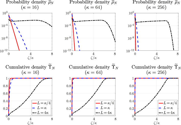
Figure 5.1: Sampling density functions $\widehat{\rho}_{N}$ in (5.2) (top) and $\widetilde{\Upsilon}_{N}$ in (5.8) (bottom) with respect to the $\kappa$-scaled evanescence parameter $\zeta$.

5.3 Inversion transform sampling

Similar to [20, sect. 8.1], $P\propto N(L)$ samples in $Y$ are generated via the Inversion Transform Sampling (ITS) technique suggested by [6, sect. 5.2]. We propose two alternative versions:

• The first one involves generating sampling sets in $[0,1]^{4}$ converging (in a suitable sense) to the uniform distribution $\mathcal{U}_{[0,1]^{4}}$ as $P$ goes to infinity, namely

  $$\{\mathbf{z}_{p}\}_{p=1}^{P},\qquad\text{with}\qquad\mathbf{z}_{p}=(z_{p,\theta_{1}},z_{p,\theta_{2}},z_{p,\psi},z_{p,\zeta})\in[0,1]^{4},\qquad p=1,...,P,$$

  and mapping them back to $Y$, to obtain sampling sets that converge to $\rho_{N}$ as $P\rightarrow\infty$, i.e.

  $$\{\mathbf{y}_{p}\}_{p=1}^{P},\qquad\text{with}\qquad\mathbf{y}_{p}=\left(\arccos{(1-2z_{p,\theta_{1}})},2\pi z_{p,\theta_{2}},2\pi z_{p,\psi},\Upsilon_{N}^{-1}(z_{p,\zeta})\right)\in Y.$$

• The second one exploits the fact that the parameters $\bm{\theta}=(\theta_{1},\theta_{2})$ should be distributed in such a way that the resulting points on the sphere converge to the uniform distribution $\mathcal{U}_{\mathbb{S}^{2}}$ as $P$ goes to infinity. This enables us to employ the spherical coordinates $\{(\widehat{\theta}_{p,1},\widehat{\theta}_{p,2})\}_{p=1}^{P}$ of nearly-uniform point sets on $\mathbb{S}^{2}$ (e.g. extremal systems [15, 23, 24, 27] in our numerical experiments) to determine the wave propagation directions, restricting the ITS technique to the evanescence parameters $(\psi,\zeta)$. Thus, we only need to generate sampling sets in $[0,1]^{2}$ that converge to the uniform distribution $\mathcal{U}_{[0,1]^{2}}$ as $P\rightarrow\infty$, i.e.

  $$\{\mathbf{z}_{p}\}_{p=1}^{P},\qquad\text{with}\qquad\mathbf{z}_{p}=(z_{p,\psi},z_{p,\zeta})\in[0,1]^{2},\qquad p=1,...,P.$$ (5.4)

  Then, we map them back to the evanescence domain $[0,2\pi)\times[0,+\infty)$, obtaining

  $$\{\mathbf{y}_{p}\}_{p=1}^{P},\qquad\text{with}\qquad\mathbf{y}_{p}=\left(\widehat{\theta}_{p,1},\widehat{\theta}_{p,2},2\pi z_{p,\psi},\Upsilon_{N}^{-1}(z_{p,\zeta})\right)\in Y.$$ (5.5)

Computing the inverse $\Upsilon_{N}^{-1}$ can be achieved through elementary root-finding methods. In our numerical experiments, we use the bisection method due to its simplicity and reliability.

$L=\kappa$			$L=4\kappa$

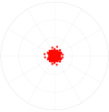
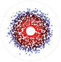
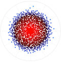
Figure 5.2: $P=N(L)$ samples for $L$ equal to $\kappa$ (left) and $4\kappa$ (right). For each value of $L$, on the left side we plot $\{(|\Re(\mathbf{d}(\mathbf{y}_{p}))|,\widehat{\theta}_{p,2})\}_{p=1}^{P}$, and on the right one $\{(|\Im(\mathbf{d}(\mathbf{y}_{p}))|,2\pi z_{p,\psi})\}_{p=1}^{P}$; see (2.6). The points are colored according to the square root of $\mu_{N}$ in (5.1). Wavenumber $\kappa=16$.

Sampling strategies

In analogy with [20, sect. 8.1], here we briefly review some sampling methods, which differ by how we generate the distribution $\{\mathbf{z}_{p}\}_{p=1}^{P}$ in $[0,1]^{n}$, for $n\in\{2,4\}$:

• Deterministic sampling: the samples are a Cartesian product of $n$ sets of equispaced points with equal number of points in each directions.

• Quasi-random sampling: the samples correspond to quasi-random low-discrepancy sequences, such as Sobol sequences [4, 14], for instance.

• Random sampling: the samples are generated randomly according to the product of $n$ uniform distributions $\mathcal{U}_{[0,1]}$.

In the following numerical experiments, we use a sampling strategy that combines quasi-random Sobol sequences [4, 14] and extremal point systems [15, 23, 24, 27], according to (5.4) and (5.5). Examples of EPW approximation sets constructed in this way are depicted in Figure 5.2. As anticipated, for smaller values of $L$, which correspond to the regime where PPWs provide a sufficient approximation, propagation vectors $\Re(\mathbf{d})$ group around $\mathbb{S}^{2}$ and evanescent vectors $\Im(\mathbf{d})$ cluster near the origin. When $L>\kappa$, the target space $\mathcal{B}_{L}$ includes Fourier modes with finer oscillations along $\partial B_{1}$ and strong radial decay away from $\partial B_{1}$, whose approximation requires EPWs with comparable properties so both $|\Re(\mathbf{d})|$ and $|\Im(\mathbf{d})|$ increase. This aligns with Figure 5.1 results.

Approximation sets

Two approximation sets can now be constructed, one consisting of sampling functionals in $\mathcal{A}$ and the other of EPWs in $\mathcal{B}$, namely

$$\Psi_{L,P}:=\,\,\Biggl{\{}\sqrt{\frac{\mu_{N}(\mathbf{y}_{p})}{P}}K_{\mathbf{y}_{p}}\Biggr{\}}_{p=1}^{P}\subset\mathcal{A}\qquad\mathrel{\mathop{\vbox{\offinterlineskip\halign{\hfil#\hfil\cr\hphantom{$\scriptstyle\mspace{8.0mu}{\bm{\mathrm{T}}_{Y}^{\scaleto{\textup{EW}\mathstrut}{5pt}}}\mspace{8.0mu}$}\cr\rightarrowfill\cr\vrule height=0.0pt,width=20.00003pt\cr\leftarrowfill\cr\hphantom{$\scriptstyle\mspace{8.0mu}{\left(\bm{\mathrm{T}}_{Y}^{\scaleto{\textup{EW}\mathstrut}{5pt}}\right)^{-1}}\mspace{8.0mu}$}\cr\kern-1.29167pt\cr} }}\limits^{\bm{\mathrm{T}}_{Y}^{\scaleto{\textup{EW}\mathstrut}{5pt}}}_{\left(\bm{\mathrm{T}}_{Y}^{\scaleto{\textup{EW}\mathstrut}{5pt}}\right)^{-1}}}\qquad\Phi_{L,P}:=\Biggl{\{}\sqrt{\frac{\mu_{N}(\mathbf{y}_{p})}{P}}\textup{EW}_{\mathbf{y}_{p}}\Biggr{\}}_{p=1}^{P}\subset\mathcal{B}.$$ (5.6)

Similarly to [20, Conj. 7.1], we conjecture that the evaluation functional sequence $\{\Psi_{L,P}\}_{L\geq 0,P\in\mathbb{N}}$ is a stable discrete approximation for the space of Herglotz densities $\mathcal{A}$, hence the EPW sequence $\{\Phi_{L,P}\}_{L\geq 0,P\in\mathbb{N}}$ is a stable discrete approximation for the space of Helmholtz solutions in the ball $\mathcal{B}$. This assertion is supported by the numerical results in section 6.

Cumulative density function approximation

The ITS technique requires to invert the cumulative density function $\Upsilon_{N}$. Although this can be easily done for every $(\bm{\theta},\psi)$, the numerical evaluation of the cumulative probability distribution (5.3) is cumbersome to implement, costly to run and numerically unstable. In fact, due to (2.34), (3.2), (3.7), and (5.1), we should compute:

$$\Upsilon_{N}(\zeta) =\int_{0}^{\zeta}\int_{\Theta}\int_{0}^{2\pi}\frac{w(\eta)}{N\mu_{N}(\bm{\theta},\psi,\eta)}\,\textup{d}\psi\textup{d}\sigma(\bm{\theta})\textup{d}\eta=2\pi|\mathbb{S}^{2}|\frac{1}{N}\sum_{\ell=0}^{L}\alpha_{\ell}^{2}\int_{0}^{\zeta}\left|\mathbf{P}_{\ell}(\eta)\right|^{2}w(\eta)\,\textup{d}\eta$$

$$=\frac{1}{N}\sum_{\ell=0}^{L}(2\ell+1)\frac{\sum_{m}\int_{0}^{\zeta}\left[\gamma_{\ell}^{m}P_{\ell}^{m}(\eta/2\kappa+1)\right]^{2}\eta^{1/2}e^{-\eta}\,\textup{d}\eta}{\sum_{m}\int_{0}^{\infty}\left[\gamma_{\ell}^{m}P_{\ell}^{m}(\eta/2\kappa+1)\right]^{2}\eta^{1/2}e^{-\eta}\,\textup{d}\eta}.$$ (5.7)

Our proposal is thus to rely on the following approximation:

$$\widetilde{\Upsilon}_{N}(\zeta):=1-\frac{1}{N}\sum_{\ell=0}^{L}(2\ell+1)\frac{Q\left(2\ell+3/2,2\kappa+\zeta\right)}{Q\left(2\ell+3/2,2\kappa\right)}\qquad\forall\zeta\in[0,+\infty),$$ (5.8)

where $Q$ is the normalized upper incomplete Gamma function [19, eq. (8.2.4)]. The approximation $\widetilde{\Upsilon}_{N}$ is obtained from (5.7) by reasoning similarly to (3.8)–(3.9): approximating $P_{\ell}^{m}$ with a monomial and controlling $\eta^{1/2}$ with $(\eta+2\kappa)^{1/2}$; the details are expounded in [10, sect. 6.3]. Compared to (5.7), this concise explicit expression is better suited for numerical evaluation. The function $\widetilde{\Upsilon}_{N}$ maintains the following essential properties: $0\leq\widetilde{\Upsilon}_{N}(\zeta)\leq 1$, $\widetilde{\Upsilon}_{N}(0)=0$ and $\lim_{\zeta\to\infty}\widetilde{\Upsilon}_{N}(\zeta)=1$. Some cumulative density functions $\widetilde{\Upsilon}_{N}$ are shown in the bottom row of Figure 5.1. When $\mathcal{A}_{L}$ only consists of elements related to the propagative regime ($L\leq\kappa$), the cumulative distributions $\widetilde{\Upsilon}_{N}$ resemble step functions, especially for large wavenumbers. However, for $L>\kappa$, these functions become more complex. Thus, while it is safe to choose only PPWs for $L\leq\kappa$, selecting EPWs becomes a non-trivial task for $L>\kappa$.

Normalization coefficient approximation

The normalization of the EPWs in $\Phi_{L,P}$ involves computing the $N\!$-term Christoffel function $\mu_{N}$, which, according to (5.1), depends on both the normalization coefficients $\alpha_{\ell}$ in (3.3) and $\mathbf{P}_{\ell}(\zeta)$ in (2.34). While the latter can be computed through recurrence relations [19, eqs. (14.7.15) and (14.10.3)], the former presents numerical challenges due to the integral in (3.7). Once again, we can address this issue by relying on [10, eq. (6.19)] and employing the approximation:

$$\alpha_{\ell}\approx\frac{\kappa^{\ell}}{e^{\kappa}}\left[\frac{2\sqrt{\pi}}{\ell!}\Gamma\left(\ell+\frac{1}{2}\right)\Gamma\left(2\ell+\frac{3}{2},2\kappa\right)\right]^{-1/2}\qquad\forall\ell\geq 0,$$ (5.9)

where we introduced the upper incomplete Gamma function [19, eq. (8.2.2)]. Alternatively, simpler normalization options are possible, such as using the $L^{\infty}$-norm on the unit ball.

Parameter tuning

The construction of the sets $\Phi_{L,P}$ requires choosing just two parameters, $L$ and $P$:

• $L$ is the Fourier truncation level. As $L$ increases, the accuracy of the approximation of $u$ by $u_{L}$, or similarly of $v=\left(\bm{\mathrm{T}}_{Y}^{\scaleto{\textup{EW}\mathstrut}{5pt}}\right)^{-1}u$ by $v_{L}$, improves.

• $P$ is the EPW approximation space dimension. When $L$ is fixed, increasing $P$ allows to enhance the accuracy of the approximation of $u_{L}$ (or $v_{L}$) by elements of $\Phi_{L,P}$ (or $\Psi_{L,P}$). The empirical evidence detailed in section 6 validates this conjecture, showing experimentally that $P$ should scale linearly with $N(L)$, with a moderate proportionality constant.

Regarding the additional parameters discussed in section 4.2, namely the number $S$ of sampling points on $\partial B_{1}$ and the SVD regularization parameter $\epsilon$, in our numerical experiments we choose $S=\lceil\sqrt{2P}\rceil^{2}$ and $\epsilon=10^{-14}$ respectively, in accordance with [10, sect. 6.1].

6 Numerical results

The numerical experiments presented in this section (see [10, Ch. 7] for more results) show the stability and accuracy achieved by the EPW sets constructed in the previous section. First, we consider the problem of the approximation of a spherical wave by either PPWs or EPWs, confirming in particular the instability result of Lemma 4.4 and showing the radical improvement offered by EPWs. Then, we explore the near-optimality of the EPW set by reconstructing random-expansion solutions and analyzing the error convergence. Numerical results on a cube show that our recipe is very effective also for non-spherical domains.

6.1 Plane wave stability

Let us examine the approximation of spherical waves by the PPW and EPW approximation sets introduced in (4.8) and (5.6), respectively. We will focus only on the case $m=0$, since the numerical results do not differ significantly varying the order $|m|\leq\ell$, as shown in [10, Fig. 3.4 and Fig. 7.1]. Once the approximation set is fixed, the same sampling matrix $A$, defined in (4.4), is used to approximate all the $b_{\ell}^{0}$ for $0\leq\ell\leq 5\kappa$.

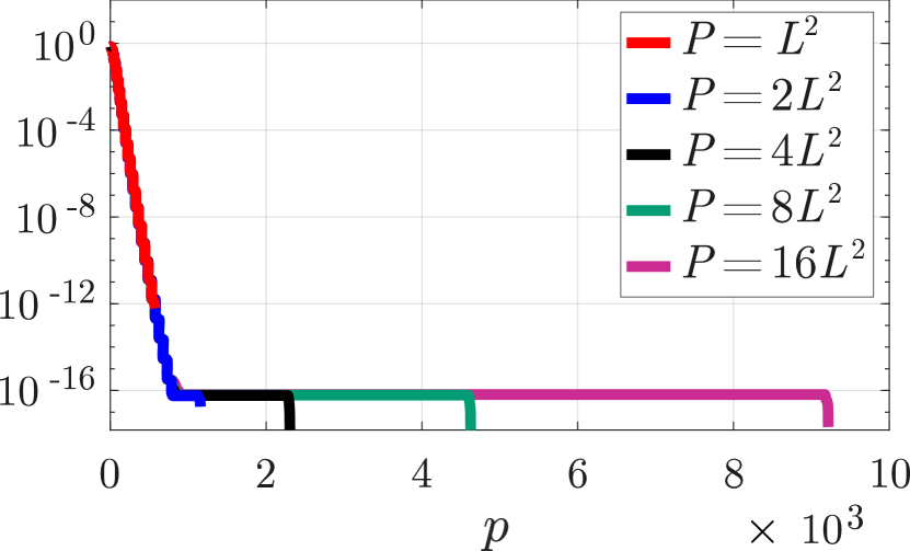
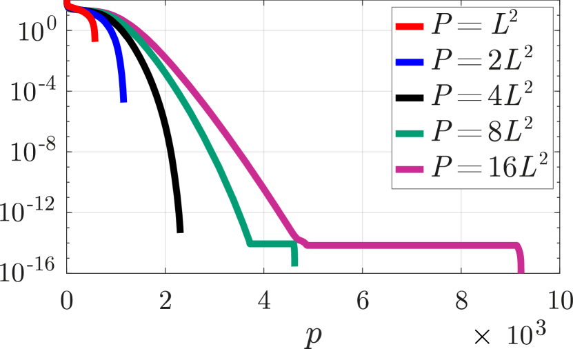
Figure 6.1: Singular values $\{\sigma_{p}\}_{p}$ of $A$ using PPWs (left) and EPWs (right). Wavenumber $\kappa=6$. Raising the number $P$ of waves, the $\epsilon$-rank of the matrix increases for EPWs but not for PPWs.

The matrix $A$ is known to be ill-conditioned: its condition number increases exponentially with the number of plane waves, a trend that can be inferred from Figure 6.1. This phenomenon is not unique to the sampling method and is observed in other experiments, see [12, sect. 4.3].

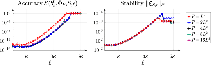
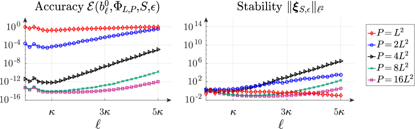
Figure 6.2: Accuracy $\mathcal{E}$ (4.7) (left) and stability $\|\bm{\xi}_{S,\epsilon}\|_{\ell^{2}}$ (right) of the approximation of spherical waves $b_{\ell}^{0}$ by both PPWs (top) and EPWs (bottom). Truncation at $L=4\kappa$ and wavenumber $\kappa=6$.

In this setting, more useful than the condition number is the concept of $\epsilon$-rank, i.e. the number of singular values of $A$ larger than $\epsilon\sigma_{\max}$, which corresponds to the dimension of the numerically achievable approximation space:

$$\epsilon\text{-rank of }A\,: =\#\{\sigma_{p}\geq\epsilon\sigma_{\max}\}=\mathrm{dim}\,\big{\{}\mathbf{b}\in\mathbb{C}^{S}\;|\;\exists\bm{\mu}\in\mathbb{C}^{|\Phi_{P}|},\ \mathbf{b}=A\bm{\mu},\ \|\bm{\mu}\|_{\ell^{2}}\leq\textstyle\frac{1}{\epsilon\sigma_{\max}}\|\mathbf{b}\|_{\ell^{2}}\big{\}}$$

$$=\mathrm{dim}\,\big{\{}u\in\operatorname{span}\Phi_{P}\;|\;\exists\bm{\mu}\in\mathbb{C}^{|\Phi_{P}|},\ u=\mathrm{T}_{P}^{\scaleto{\textup{PW}\mathstrut}{5pt}}\bm{\mu},\ \|\bm{\mu}\|_{\ell^{2}}\leq\textstyle\frac{1}{\epsilon\sigma_{\max}}\|\mathbf{b}(u)\|_{\ell^{2}}\big{\}},$$

where $\mathbf{b}(u)\in\mathbb{C}^{S}$ is the boundary sampling vector of $u$, as in (4.4).

The approximation results are shown in Figure 6.2. The left panels show the relative residual $\mathcal{E}$ in (4.7) as a measure of the approximation accuracy. On the right panels, the coefficient size $\|\bm{\xi}_{S,\epsilon}\|_{\ell^{2}}$ indicates the stability of the approximations.

Propagative plane waves

Let us focus on the PPW approximation sets $\Phi_{P}$ in (4.8).

Figure 6.1 shows that the $\epsilon$-rank of the matrix $A$ does not increase as $P$ is raised: more PPWs do not lead to the stable approximation of more Helmholtz solutions.

In Figure 6.2 (top), three distinct regimes are observed:

• For the propagative modes, i.e. for spherical waves with mode number $\ell\leq\kappa$, the approximation is accurate ($\mathcal{E}<10^{-13}$) and the size of the coefficients is moderate ($\|\bm{\xi}_{S,\epsilon}\|_{\ell^{2}}<10$).

• For mode numbers $\ell$ larger than the wavenumber $\kappa$, the norm of the coefficient vector grows exponentially in $\ell$ and the accuracy decreases proportionally.

• At a certain point (roughly between $\ell=4\kappa$ and $\ell=5\kappa$ in this numerical experiment), the exponential growth of the coefficients completely destroys the stability of the approximation and we are unable to approximate the target $b_{\ell}^{0}$ with any significant accuracy.

As in [20, sect. 4.4], increasing $P$ does not enhance accuracy beyond a certain threshold. Despite the matrix $A$ being extremely ill-conditioned, accuracy for propagative modes $\ell\leq\kappa$ reaches machine precision. On the other hand, evanescent modes with larger mode numbers $\ell\geq 4\kappa$ maintain an error of $\mathcal{O}(1)$, thanks to the simple regularization technique outlined in section 4.2. In line with Theorem 4.5, any regularization technique can mitigate but not eliminate the inherent instability of Trefftz methods employing PPWs. Even with regularization, achieving accurate approximation of evanescent modes within a given floating-point precision remains unattainable.

Evanescent plane waves

Now, let us consider the EPW approximation sets $\Phi_{L,P}$ in (5.6) instead. In Figure 6.2 (bottom), we fix the truncation parameter at $L=4\kappa$. With enough waves, i.e. $P$ large enough, all modes $\ell\leq L=4\kappa$ are approximated to near machine precision. This encompasses both propagative modes $\ell\leq\kappa$, which were already well-approximated using only PPWs, and evanescent modes $\kappa<\ell\leq L=4\kappa$, for which purely PPWs provided poor or no approximation. Moreover, higher-degree modes $L=4\kappa<\ell\leq 5\kappa$ are also accurately approximated. The coefficient norms $\|\bm{\xi}_{S,\epsilon}\|_{\ell^{2}}$ in the approximate expansions are moderate, differing from the propagative case. From Figure 6.1, one understands that if $P$ is large enough, the condition number of the matrix $A$ is comparable for both PPWs and EPWs. Improved accuracy for evanescent modes does not arise from better conditioning but from a higher $\epsilon$-rank: from less than $10^{3}$ for PPWs to around $5\times 10^{3}$ for EPWs in the case $P=16L^{2}$. Raising the truncation parameter $L$ allows to increase the $\epsilon$-rank of $A$: more solutions can be approximated with bounded coefficients by the EPWs.

6.2 Approximation of random-expansion solutions

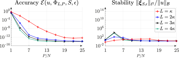
Figure 6.3: Accuracy $\mathcal{E}$ (4.7) (left) and stability $\|\bm{\xi}_{S,\epsilon}\|_{\ell^{2}}/\|u\|_{\mathcal{B}}$ (right) of the approximation of solution $u$ in (6.1) by $P$ EPWs. The horizontal axis represents the ratio $P/N(L)$, where $N(L)=(L+1)^{2}$ is the dimension of the space $\mathcal{B}_{L}$, to which $u$ belongs. Wavenumber $\kappa=6$.

We test the numerical procedure presented in section 5 by reconstructing a solution of the form

$$u:=\sum_{\ell=0}^{L}\sum_{m=-\ell}^{\ell}\widehat{u}_{\ell}^{m}[\max\{1,\ell-\kappa\}]^{-1}b_{\ell}^{m}\in\mathcal{B}_{L},$$ (6.1)

where the coefficients $\widehat{u}_{\ell}^{m}$ are independent, normally-distributed random numbers. This is a challenging scenario, as the coefficients of any element in $\mathcal{B}$ decay in modulus as $o(\ell^{-1})$ for large $\ell$.

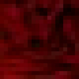
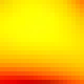
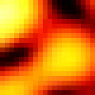
Figure 6.4: Absolute errors of the approximation of a solution $u$ in (6.1) with $\kappa=5$ and $L=5\kappa=25$, so that $u$ is defined by $N(L)=676$ random parameters. The error corresponds to the use of $P=4(L+1)^{2}=2704$ plane waves, either PPWs in $\Phi_{P}$ from (4.8) (left) or EPWs in $\Phi_{L,P}$ from (5.6) (right). Note the different ranges in the color scales. The absolute errors are plotted both on $B_{1}\cap\{\mathbf{x}=(x,y,z):xyz=0\}$ (top) and on the unit sphere $\partial B_{1}$ (bottom).

In Figure 6.3 we display the relative residual $\mathcal{E}$ and the coefficient size $\|\bm{\xi}_{S,\epsilon}\|_{\ell^{2}}/\|u\|_{\mathcal{B}}$ with respect to the ratio $P/N(L)$, that is the approximation set dimension divided by the dimension of the space of the possible solutions in (6.1). The numerical results suggest that the size of the approximation set $P$ should vary linearly with respect to $N(L)$: when $L$ is large enough (e.g. $L\geq 2\kappa$), the decays are largely independent of $L$. The $\Phi_{L,P}$ approximation sets (5.6) appear close to optimal, requiring only $\mathcal{O}(N)$ DOFs with a moderate proportionality constant to approximate $N$ spherical modes with reasonable accuracy. Here, for $L\geq 2\kappa$, $P=10N$ suffices to obtain $\mathcal{E}\leq 10^{-12}$.

Figure 6.4 shows the absolute errors resulting from approximating a solution of the form (6.1), with wavenumber $\kappa=5$ and truncation parameter $L=5\kappa=25$, by $P=4(L+1)^{2}=2704$ plane waves, whether they are PPWs or EPWs. For other plots of this kind see [10, sect. 7.2].

The error from PPWs is much larger than that from EPWs (around $8$ orders of magnitude in $L^{\infty}$-norm) and is mainly concentrated near the boundary. This happens because EPWs can effectively capture the higher Fourier modes of Helmholtz solutions, which PPWs cannot achieve.

The number of DOFs per wavelength $\lambda=2\pi/\kappa$ employed in each direction can be estimated by $\lambda\sqrt[3]{3P/4\pi}$, which is approximately $11$ in Figure 6.4. In low-order methods, a common rule of thumb is around $6\sim 10$ DOFs per wavelength for $1\sim 2$ digits of accuracy. Remarkably, thanks to the selected EPWs, merely a fraction above this count yields more than $8$ digits of accuracy.

6.3 Cubic domain

To conclude, we present some numerical results in a cubic domain to show that the approximation set we developed, based on the analysis of the unit ball $B_{1}$, perform well on other geometries as well. Additional results involving tetrahedrons can be found in [10, sect. 7.4]. Let $Q_{1}$ denote the cube with edges aligned to the Cartesian axes and inscribed within the unit sphere, and consider the problem of the approximation of the Helmholtz fundamental solution, namely

$$\mathbf{x}\mapsto\frac{1}{4\pi}\frac{e^{i\kappa|\mathbf{x}-\mathbf{s}|}}{|\mathbf{x}-\mathbf{s}|}\qquad\forall\mathbf{x}\in Q_{1},\qquad\text{where}\qquad\mathbf{s}\in\mathbb{R}^{3}\setminus\overline{Q_{1}}.$$ (6.2)

We exploit the approximation recipe of section 4.2 for the circumscribed ball, using equispaced Dirichlet data points on $\partial Q_{1}$ and solving an oversampled linear system with a regularized SVD. Specifically, using evenly spaced sampling points on $\partial Q_{1}$ allows us to select uniform weights in (4.4). The truncation parameter $L$ is computed from $P$ as $L:=\max\{\lceil\kappa\rceil,\lfloor\sqrt{P/10}\rfloor\}$, based on the numerical results of section 6.2. Moreover, the EPWs in (5.6) are normalized to have unit $L^{\infty}$-norm on $\partial Q_{1}$, this being the sole deviation from the sets used for spherical geometry.

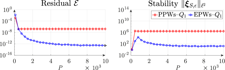
Figure 6.5: Residual $\mathcal{E}$ (4.7) (left) and stability $\|\bm{\xi}_{S,\epsilon}\|_{\ell^{2}}$ (right) of the approximation of the fundamental solution (6.2) in the cube $Q_{1}$ with $\mathbf{s}=(1/\sqrt{3}+2\lambda/3,0,0)$, so that $\textup{dist}(\mathbf{s},\partial Q_{1})=2\lambda/3$. The PPW and EPW approximation sets $\Phi_{P}$ and $\Phi_{L,P}$ are compared. We report the convergence for increasing size of the approximation set $P$. Wavenumber $\kappa=5$.

In Figure 6.5 we report the convergence of the plane wave approximations, either PPW or EPW, for increasing size of the approximation set $P$. When PPWs are employed, the residual of the linear system initially reduces swiftly with increasing $P$, but eventually plateaus, well before reaching machine precision, due to the rapid growth of the coefficients. Conversely, when using EPW approximation sets, the residual converges to machine precision and the coefficient size remains reasonable. In fact, by using EPWs, the truncation parameter $L$, and consequently the number of approximated modes, grows concurrently with $P$, providing an increasingly accurate approximation. In contrast, PPWs are only able to stably approximate propagative modes. Once this content is correctly captured, further increasing the discrete space dimension only brings instability, due to the impossibility of approximating high Fourier modes. Figure 6.6 shows the absolute errors in approximating a fundamental solution (6.2) by $P=2704$ plane waves, either PPWs or EPWs. For similar plots, refer to [10, sect. 7.4].

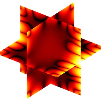
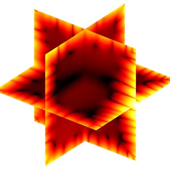
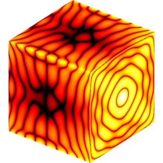
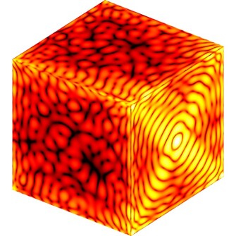
Figure 6.6: Absolute errors of the approximation of the fundamental solution (6.2) with $\kappa=5$ and $\mathbf{s}\in\mathbb{R}^{3}\setminus\overline{Q_{1}}$ so that $\textup{dist}(\mathbf{s},\partial Q_{1})=\lambda/3$. The solution is approximated using $P=2704$ plane waves, either PPWs in $\Phi_{P}$ from (4.8) (left) or EPWs in $\Phi_{L,P}$ from (5.6) (right). The absolute errors are plotted on both $Q_{1}\cap\{\mathbf{x}=(x,y,z):xyz=0\}$ (top) and the boundary $\partial Q_{1}$ (bottom).

These results highlight the potential of the proposed numerical method for plane wave approximations and Trefftz schemes, particularly since it is not optimized for cubic geometries (except for the $L^{\infty}$ normalization at the boundary). We are confident that our numerical recipe could be refined by defining rules tailored to the specific underlying geometries, thereby paving the way for even more effective approximation strategies.

7 Conclusions

This paper extends the analysis of plane wave approximation properties from 2D to 3D. As expected, also in 3D PPWs are not suited for stably approximating high-frequency Fourier modes, whose integral representation as a continuous superposition of PPWs features a density function that blows up with the mode number. This is reflected in large expansion coefficients associated with finite PPW sets and constitutes the fundamental source of numerical instability in standard plane-wave based Trefftz schemes. Conversely, any Helmholtz solution in the unit ball can be exactly represented as a continuous superposition of EPWs with a unique bounded density function. We propose a numerical recipe that carefully selects suitable finite EPW sets, leading to accurate and numerically stable discrete approximations. Future research aims to explore more diverse geometries and the use of EPWs in Trefftz Discontinuous Galerkin schemes.

References

- [1] Mark J. Ablowitz and Athanassios S. Fokas “Complex variables: introduction and applications. ed”, Cambridge Texts in Applied Mathematics Cambridge University Press, Cambridge, 2003 DOI: 10.1017/CBO9780511791246
- [2] Ben Adcock and Daan Huybrechs “Frames and numerical approximation” In SIAM Rev. 61.3, 2019, pp. 443–473 DOI: 10.1137/17M1114697
- [3] Ben Adcock and Daan Huybrechs “Frames and numerical approximation II: Generalized sampling” In J. Fourier Anal. Appl. 26.6, 2020, pp. Paper No. 87\bibrangessep34 DOI: 10.1007/s00041-020-09796-w
- [4] Paul Bratley and Bennett L Fox “Algorithm 659: Implementing Sobol’s quasirandom sequence generator” In ACM Trans. Math. Software 14.1 ACM New York, NY, USA, 1988, pp. 88–100
- [5] Ole Christensen “An introduction to frames and Riesz bases”, Applied and Numerical Harmonic Analysis Birkhäuser/Springer, [Cham], 2016 DOI: 10.1007/978-3-319-25613-9
- [6] Albert Cohen and Giovanni Migliorati “Optimal weighted least-squares methods” In SMAI J. Comput. Math. 3, 2017, pp. 181–203 DOI: 10.5802/smai-jcm.24
- [7] David Colton and Rainer Kress “Inverse acoustic and electromagnetic scattering theory” 93, Applied Mathematical Sciences Springer, New York, 2013 DOI: 10.1007/978-1-4614-4942-3
- [8] Arthur Erdélyi, Wilhelm Magnus, Fritz Oberhettinger and Francesco G. Tricomi “Higher transcendental functions. Vols. I, II” Based, in part, on notes left by Harry Bateman McGraw-Hill Book Co., Inc., New York-Toronto-London, 1953
- [9] X.. Feng, P. Wang, W. Yang and G.. Jin “High-precision evaluation of Wigner’s matrix by exact diagonalization” In Phys. Rev. E 92 American Physical Society, 2015, pp. 043307 DOI: 10.1103/PhysRevE.92.043307
- [10] Nicola Galante “Evanescent Plane Wave Approximation of Helmholtz Solutions in Spherical Domains” Master Thesis, University of Pavia, 2023 arXiv:2305.02175 [math.NA]
- [11] Jerrad Hampton and Alireza Doostan “Coherence motivated sampling and convergence analysis of least squares polynomial Chaos regression” In Comput. Methods Appl. Mech. Engrg. 290, 2015, pp. 73–97 DOI: 10.1016/j.cma.2015.02.006
- [12] Ralf Hiptmair, Andrea Moiola and Ilaria Perugia “A survey of Trefftz methods for the Helmholtz equation” In Building bridges: connections and challenges in modern approaches to numerical partial differential equations 114, Lect. Notes Comput. Sci. Eng. Springer, [Cham], 2016, pp. 237–278
- [13] Daan Huybrechs and Anda-Elena Olteanu “An oversampled collocation approach of the wave based method for Helmholtz problems” In Wave Motion 87, 2019, pp. 92–105 DOI: 10.1016/j.wavemoti.2018.06.001
- [14] Stephen Joe and Frances Y. Kuo “Remark on Algorithm 659: implementing Sobol’s quasirandom sequence generator” In ACM Trans. Math. Software 29.1, 2003, pp. 49–57 DOI: 10.1145/641876.641879
- [15] Jordi Marzo and Joaquim Ortega-Cerdà “Equidistribution of Fekete points on the sphere” In Constr. Approx. 32.3, 2010, pp. 513–521 DOI: 10.1007/s00365-009-9051-5
- [16] Giovanni Migliorati and Fabio Nobile “Stable high-order randomized cubature formulae in arbitrary dimension” In J. Approx. Theory 275, 2022, pp. Paper No. 105706\bibrangessep30 DOI: 10.1016/j.jat.2022.105706
- [17] A. Moiola, R. Hiptmair and I. Perugia “Plane wave approximation of homogeneous Helmholtz solutions” In Z. Angew. Math. Phys. 62.5, 2011, pp. 809–837 DOI: 10.1007/s00033-011-0147-y
- [18] Jean-Claude Nédélec “Acoustic and electromagnetic equations” Integral representations for harmonic problems 144, Applied Mathematical Sciences Springer-Verlag, New York, 2001 DOI: 10.1007/978-1-4757-4393-7
- [19] “NIST Digital Library of Mathematical Functions” F. W. J. Olver, A. B. Olde Daalhuis, D. W. Lozier, B. I. Schneider, R. F. Boisvert, C. W. Clark, B. R. Miller, B. V. Saunders, H. S. Cohl, and M. A. McClain, eds., Release 1.1.9 of 2023-03-15 URL: http://dlmf.nist.gov/
- [20] Emile Parolin, Daan Huybrechs and Andrea Moiola “Stable approximation of Helmholtz solutions in the disk by evanescent plane waves” In ESAIM Math. Model. Numer. Anal. 57.6, 2023, pp. 3499–3536 DOI: 10.1051/m2an/2023081
- [21] Vern I. Paulsen and Mrinal Raghupathi “An introduction to the theory of reproducing kernel Hilbert spaces” 152, Cambridge Studies in Advanced Mathematics Cambridge University Press, Cambridge, 2016 DOI: 10.1017/CBO9781316219232
- [22] J. Pendleton “Euler angle geometry, helicity basis vectors, and the Wigner D-function addition theorem” In American Journal of Physics 71.12 American Association of Physics Teachers, 2003, pp. 1280–1291 DOI: 10.1119/1.1615525
- [23] Manfred Reimer “Constructive theory of multivariate functions” Bibliographisches Institut, Man-nheim, 1990, pp. 280
- [24] Ian H. Sloan and Robert S. Womersley “Extremal systems of points and numerical integration on the sphere” In Adv. Comput. Math. 21.1-2, 2004, pp. 107–125 DOI: 10.1023/B:ACOM.0000016428.25905.da
- [25] Alan D. Sokal “How to generalize (and not to generalize) the Chu–Vandermonde identity” In The American Mathematical Monthly 127.1 Informa UK Limited, 2019, pp. 54–62 DOI: 10.1080/00029890.2020.1668707
- [26] D.. Varshalovich, A.. Moskalev and V.. Khersonskiı “Quantum theory of angular momentum” Irreducible tensors, spherical harmonics, vector coupling coefficients, symbols, Translated from the Russian World Scientific Publishing Co., Inc., Teaneck, NJ, 1988 DOI: 10.1142/0270
- [27] Robert S. Womersley and Ian H. Sloan “How good can polynomial interpolation on the sphere be?” In Adv. Comput. Math. 14.3, 2001, pp. 195–226 DOI: 10.1023/A:1016630227163