MX: Enhancing RISC-V’s Vector ISA for Ultra-Low Overhead, Energy-Efficient Matrix Multiplication

Abstract

Dense Matrix Multiplication (MatMul) is arguably one of the most ubiquitous compute-intensive kernels, spanning linear algebra, DSP, graphics, and machine learning applications. Thus, MatMul optimization is crucial not only in high-performance processors but also in embedded low-power platforms. Several Instruction Set Architectures (ISAs) have recently included matrix extensions to improve MatMul performance and efficiency at the cost of added matrix register files and units.

In this paper, we propose Matrix eXtension (MX), a lightweight approach that builds upon the open-source RISC-V Vector (RVV) ISA to boost MatMul energy efficiency. Instead of adding expensive dedicated hardware, MX uses the pre-existing vector register file and functional units to create a hybrid vector/matrix engine at a negligible area cost ($\mathbf{<3\%}$), which comes from a compact near-FPU tile buffer for higher data reuse, and no clock frequency overhead. We implement MX on a compact and highly energy-optimized RVV processor and evaluate it in both a Dual- and 64-Core cluster in a 12-nm technology node. MX boosts the Dual-Core’s energy efficiency by 10% for a double-precision 64x64x64 matrix multiplication with the same FPU utilization ($\mathbf{\approx 97\%}$) and by 25% on the 64-Core cluster for the same benchmark on 32-bit data, with a 56% performance gain.

I Introduction

The exponential growth of the computational requirements in Machine Learning (ML) and Artificial Intelligence (AI) applications is a major challenge for hardware architects. The rise of application-specific accelerators [1] and single instruction, multiple data (SIMD) programmable systems [2] demonstrates the need for novel architectures able to cope with the rising computational demand. Furthermore, AI/ML applications also found their way into edge computing, with benefits such as higher privacy, user personalization, and lower power consumption. However, edge-AI/ML systems have the additional challenge of balancing large computational demands against a very tight power envelope and minimal area footprint. The quest for energy efficiency and cost (i.e., area) minimization is even more pressing today since ML/AI computation at the edge does not only involve inference but also training in the so-called AI on Edge [3].

Matrix Multiplication (MatMul) is a cornerstone in ML and AI, and essential in scientific computing, graphics, and Digital Signal Processing (DSP). The importance of MatMul is testified by market-leading companies, such as Google, which developed the first Tensor-Processing Unit (TPU) in 2015 to accelerate matrix operations [4] and updated it in 2018 with an edge-oriented version achieving $4\text{\,}\mathrm{TOPS}$ within a $2\text{\,}\mathrm{W}$ power envelope [5]. As with other Domain-Specific Accelerators (DSAs) for specific neural-network tasks [6], the TPU is an added resource to which a general-purpose processor offloads the workload (for example, through a PCIe interface). This brings an area and power overhead that is not affordable in constrained systems at the edge, especially when they need to compute non-AI tasks as well. Moreover, an excessively specialized accelerator risks becoming useless when the ML/AI algorithm evolves.

Most proprietary Instruction Set Architectures (ISAs) offer dedicated matrix extensions, such as Arm’s Scalable Matrix Extension (SME), Intel Advanced Matrix Extension (AMX), and IBM Matrix-Multiply Assist (MMA). Unluckily, the micro-architectural details of the implementations remain company secrets. So far, the RISC-V open-source ISA features only a vector extension (RISC-V Vector (RVV)), even though researchers developed multiple unofficial AI/matrix extensions. Still, they add tightly coupled matrix units [7] or a new matrix register file [8] used only during matrix operations, which add area and power consumption.

RVV recently showed to be a valid solution to efficiently accelerate MatMul while keeping a well-known programming model to handle diverse data-parallel workloads, also in the embedded domain [9]. Vector processors execute multiple operations with one instruction, amortizing its fetch/decode cost. Moreover, they feature a Vector Register File (VRF) to buffer the vector elements, decreasing the accesses to memory without changing the computational balance for the architecture [10]. Even if the VRF helps decrease the power associated with the memory accesses, it is an additional block at the bottom of the memory hierarchy, one of the key drivers for performance and energy efficiency [11]. Its size can be way larger than the one of a scalar register file, and it is usually connected to multiple functional units in parallel, which leads to energy-hungry interconnects. Hence, the VRF access-related energy is usually non-negligible [12, 9].

With this paper, we present Matrix eXtension (MX), a non-intrusive ISA extension to RVV that creates a general-purpose hybrid matrix/vector architecture with minimal area impact and superior energy efficiency. To cut the power consumption, we reduce the expensive accesses to/from the VRF by featuring a software-transparent lightweight accumulator close to the processing units. MX does not add a matrix unit to the architecture but re-uses the already available processing resources to keep the area and energy overhead at its minimum and exploit the energy efficiency savings that come from the reduced VRF accesses.

To validate MX across multiple domains, we add MX to a constrained embedded Dual-Core cluster built upon the open-source energy-optimized RVV-based Spatz [9] vector processor and to a scaled-up MemPool architecture [13] with 64 Spatz processors and implement both systems in a competitive 12-nm technology. We provide a quantitative justification of the energy savings and a detailed power, performance, and area (PPA) analysis on matrix multiplications on different data precisions, finding that our matrix extension can boost not only energy efficiency but also performance.

With this paper, we present the following contributions:

• We define MX, a lightweight and non-intrusive ISA extension based on RVV 1.0 aimed at supporting memory and computational operations directly on matrices. MX reduces the power consumption of the architecture with similar or better performance by introducing a near-Floating Point Unit (FPU) tile buffer, a per-vector-element broadcast system, and minimal modifications to the Vector Load/Store Unit (VLSU).

• We provide a theoretical justification of the benefits that the ISA has on the power consumption when executing a matrix multiplication kernel, effectively reducing the expensive VRF accesses.

• We implement MX on a constrained Dual-Core and a complex 64-core clusters based on the energy-efficient RVV vector processor Spatz, and characterize MX’s impact on performance and PPA metrics in a 12-nm technology. For less than 3% area overhead, we get a maximum of 56% and 25% performance and energy efficiency gains, respectively.

II Analysis

In the following, we discuss the tiling of a General Matrix Multiply (GEMM) problem through a multi-level memory hierarchy. When C is a zero matrix, GEMM becomes a MatMul.

$$D_{M\times N}=A_{M\times K}\cdot B_{K\times N}+C_{M\times N}$$ (1)

For convenience, let us consider a memory hierarchy composed of a memory, a VRF, and a near-FPU buffer. The memory connects to the VRF, which is connected to a buffer that feeds the FPUs, as reported in Figure 1. The following analysis can be easily extended to memory hierarchies with a different number of levels.

II-A The tiling problem

The lower level of the hierarchy is usually not large enough to keep the input and output matrices all at once. Therefore, the matrices are divided into chunks (tiles), and the hardware works on one output tile at a time, and the outer product algorithm is often used to maximize parallelism. The number of elements transferred between two consecutive levels of the hierarchy impacts both performance and power consumption and depends on how the matrices are tiled. Usually, the number of transfers is partially encoded in the arithmetic intensity, i.e., the total number of operations divided by the total number of Bytes transferred between the memory and the core.

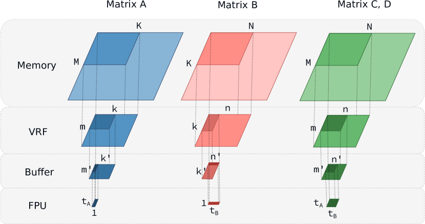
Figure 1: The tiling problem over a memory hierarchy composed of three levels, ending with the processing elements (FPUs).

In the following, we provide equations to fine-grain count how many memory accesses happen between each pair of consecutive levels of the hierarchy. Each equation contains four terms, which correspond to 1) the elements of matrix A, 2) the elements of matrix B, 3) the elements of matrix C (or D) from the upper level to the lower one (load/fetch), and 4) the elements of the matrix D from the lower level back to the upper one (store/write-back).

In the most generic scenario, without buffering the output tile in the VRF for more than $k$ updates, the number of elements moved between the memory and the VRF is:

$$\#Elm^{MEM}_{VRF}=\frac{N}{n}MK+\frac{M}{m}NK+\frac{K}{k}MN+\frac{K}{k}MN$$ (2)

Where the A, B, and D (C) matrices stored in memory have sizes $MK,NK,MN$, and we tile the problem between the memory and the VRF with tiles of size $mk,nk,mn$.

For each matrix tile, the number of elements exchanged between the VRF and the buffer is:

$$\#Elm^{VRF}_{BUF}=\frac{n}{n^{\prime}}mk+\frac{m}{m^{\prime}}nk+\frac{k}{k^{\prime}}mn+\frac{k}{k^{\prime}}mn$$ (3)

Where the tiles stored in the VRF have sizes $mk,nk,mn$, and we sub-tile the problem between the VRF and the buffer with sub-tiles of size $m^{\prime}k^{\prime},n^{\prime}k^{\prime},m^{\prime}n^{\prime}$.

For each matrix sub-tile, the number of elements exchanged between the buffer and the FPUs is:

$$\#Elm^{BUF}_{FPU}=\frac{n^{\prime}}{t_{B}}m^{\prime}k^{\prime}+\frac{m^{\prime}}{t_{A}}n^{\prime}k^{\prime}+k^{\prime}m^{\prime}n^{\prime}+k^{\prime}m^{\prime}n^{\prime}$$ (4)

Where the sub-tiles stored in the buffer have sizes $m^{\prime}k^{\prime},n^{\prime}k^{\prime},m^{\prime}n^{\prime}$, and we access $t_{A}$ and $t_{B}$ elements from tiles A and B, respectively.

II-B Total number of transfers

To get the total number of transfers between each pair of hierarchy levels, we need to take into account how many output tiles and sub-tiles we calculate throughout the program.

Memory and VRF

In the most generic case, we load the C (first iteration) and D (from the second iteration on) tiles from memory before consuming the input $mk,nk$-sized tiles, and we store the D tile back to memory after $k$ updates. Without inter-k-tile buffering in the VRF, we load $(\frac{K}{k})\frac{M}{m}\frac{N}{n}$ output tiles with size $mn$ from the memory to the VRF, and we store back the same amount. If we buffer the output tiles until they are completely calculated over the whole K dimension, the formula simplifies to $\frac{M}{m}\frac{N}{n}$. Instead, we load a total of $\frac{K}{k}\frac{M}{m}\frac{N}{n}$ input A and B tiles, with sizes $mk,nk$.

VRF and buffer

The $m^{\prime}n^{\prime}$ output sub-tiles of a tile are fetched for $(\frac{k}{k^{\prime}})\frac{m}{m^{\prime}}\frac{n}{n^{\prime}}$ times from the VRF before consuming the input $m^{\prime}k^{\prime},n^{\prime}k^{\prime}$-sized sub-tiles in the buffer, and written-back to the VRF for the same number of times if there is no inter-k-tile buffering in the buffer. Instead, the input A and B sub-tiles, with sizes $m^{\prime}k^{\prime},n^{\prime}k^{\prime}$, are loaded $\frac{K}{k}\frac{M}{m}\frac{N}{n}$ times. If we keep into account how many times each tile is loaded/stored from/to memory, these formulas become $(\frac{K}{k})(\frac{k}{k^{\prime}})\frac{M}{m^{\prime}}\frac{N}{n^{\prime}}$ for the sub-tiles fetch, the same amount for the sub-tiles writes-back, and $\frac{K}{k^{\prime}}\frac{M}{m^{\prime}}\frac{N}{n^{\prime}}$ for the A and B sub-tiles fetch.

We summarize all the transfers across the hierarchy in Table I.

Table I: Number of accesses between consecutive levels of the memory hierarchy.

Ref.	Metric	A ($\downarrow$)	B ($\downarrow$)	C, D ($\downarrow$)	D ($\uparrow$)
1)	$\mathrm{\#Elm^{MEM}_{VRF}}$	$\mathrm{\frac{N}{n}MK}$	$\mathrm{\frac{M}{m}NK}$	$\mathrm{\frac{K}{k}MN}$	$\mathrm{\frac{K}{k}MN}$
2)	$\mathrm{\#Elm^{VRF}_{BUF}}$	$\mathrm{\frac{N}{n^{\prime}}MK}$	$\mathrm{\frac{M}{m^{\prime}}NK}$	$\mathrm{\frac{k}{k^{\prime}}\frac{K}{k}MN}$	$\mathrm{\frac{k}{k^{\prime}}\frac{K}{k}MN}$
3)	$\mathrm{\#Elm^{BUF}_{FPU}}$	$\mathrm{\frac{N}{t_{B}}MK}$	$\mathrm{\frac{M}{t_{A}}NK}$	$\mathrm{k^{\prime}\frac{k}{k^{\prime}}\frac{K}{k}MN}$	$\mathrm{k^{\prime}\frac{k}{k^{\prime}}\frac{K}{k}MN}$

1. $\downarrow/\uparrow$ indicate transfers to a lower/higher level of the memory.

II-C Optimizations

Inter-k-buffering

If the output tile (sub-tile) is buffered in the VRF (buffer) until the whole K (k) dimension is traversed and the whole output tile (sub-tile) is ready, we can simplify the equations above. If the buffering happens in the VRF, $\frac{K}{k}=1$ in Table I Ref. 1), while if it happens in the buffer until the whole $K$ dimension, $\frac{K}{k}\frac{k}{k^{\prime}}=1$, in Table I Ref. 2) (if the buffering only happens until the whole $k$ dimension is traversed, $\frac{k}{k^{\prime}}=1$).

Inter-k-buffering is ultimately limited by the size of the lower memory level, which should be able to host the whole output tile (sub-tile) for the whole computation on the $K$ ($k$) dimension. Therefore, keeping the output tile in the buffer for the whole $K$ dimension requires that $m=m^{\prime},n=n^{\prime}$. On the other hand, relaxing this constraint, e.g. $m=m^{\prime},n=B\times n^{\prime}$, allows for fewer overall transfers between the memory and the VRF. In this case, the inter-k-buffering can be done only between the memory and the VRF.

C-tile reset

When C is a zero matrix, it’s possible to avoid loading it from memory and initialize the VRF with zeroes or reset the buffer. If we use inter-k-buffering and the zero initialization is applied to the VRF and the buffer, the third term of the equations related to the load/fetch of matrix C, D, becomes zero in Table I Ref. 1) and 2), respectively.

III MX Implementation

III-A ISA Extension

We implement MX in Spatz [9], an open-source, RVV-based, highly-optimized compact vector processor, targeting minimal area and power overhead. Thus, we do not add any dedicated matrix units or software-addressable registers, as shown in Figure 2. MX adds three configure instructions (msettile[m,n,k]), three memory instructions (mld.[a,b], mst.c), and two computation instructions (mx[f]macc). The first three instructions set up the sub-tile sizes $m^{\prime},n^{\prime},k^{\prime}$ on which the matrix instructions operate ($m^{\prime}k^{\prime}=vl$, $m^{\prime}n^{\prime}\leq vl$, and $vl$ is the vector length in elements). We enhance the VLSU to enable matrix load and store operations, which are composed of multiple unit- and non-unit-stride memory operations already supported by Spatz. The new memory instructions are introduced to load tiles from matrix A and B and to store the computed tile back to memory, while the two computational instructions perform a MatMul between the two $m^{\prime}k^{\prime}$ and $k^{\prime}n^{\prime}$ sub-tiles, storing the resulting $m^{\prime}n^{\prime}$ sub-tile in the VRF. Close to the FPUs, we introduce a tiny broadcast block consisting only of a register and some multiplexers to broadcast single elements from the A tile across multiple elements of tile B. This block increases the data reuse of tile A at a minimal cost. Finally, we implement a latch-based result tile buffer in the vector functional unit (VFU) to reduce energy consumption by minimizing VRF accesses by intermediate result accumulation, limiting the buffer size to $\frac{1}{8}$ of the VRF size (i.e., $BUF_{size}=256B$) to maintain low energy and area overhead. Since Spatz’s VLSU has four parallel memory ports and the buffer is constrained in size, $m^{\prime},n^{\prime},k^{\prime}\in\{4,8\}$.

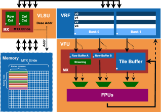
Figure 2: Spatz’s VLSU, VRF, and VFU with MX architectural schematic.

III-B MX Benefits

Table II summarizes the number of elements transferred between consecutive memory hierarchies for a baseline vector-only MatMul and a MX-ready MatMul . The baseline employs a traditional scalar-vector algorithm to load m scalar elements from the input matrix A and an n-long vector from matrix B. The MX-ready configuration loads A tiles with size $m^{\prime}k^{\prime}$ and B tiles with size $n^{\prime}k^{\prime}$. While the MX algorithm does not further sub-tile the tiles on $m$ or $k$ ($\textit{m'}=\textit{m}$ and $\textit{k'}=\textit{k}$), it sub-tiles along n such that $\textit{n}=B\times\textit{n'}$, where $B\in\{2,4\}$. In the following, we highlight the benefits brought by the MX algorithm.

Table II: Data Transfers: MX-ready vs Baseline.

Config	Metric	A ($\downarrow$)	B ($\downarrow$)	C, D ($\downarrow$)	D ($\uparrow$)
Baseline${}^{\mathrm{\ref{tnote:xrf}}}$	$\mathrm{\#Elm^{MEM}_{VRF}}$	$\mathrm{\frac{N}{n}MK}$	$\mathrm{\frac{M}{m}NK}$	$\mathrm{0}$	$\mathrm{MN}$
Baseline${}^{\mathrm{\ref{tnote:xrf}}}$	$\mathrm{\#Elm^{VRF}_{FPU}}$	$\mathrm{\frac{N}{F}MK}$	$\mathrm{MNK}$	$\mathrm{KMN}$	$\mathrm{KMN}$
MX	$\mathrm{\#Elm^{MEM}_{VRF}}$	$\mathrm{\frac{N}{B\times n^{\prime}}MK}$	$\mathrm{\frac{M}{m^{\prime}}NK}$	$\mathrm{0}$	$\mathrm{MN}$
MX	$\mathrm{\#Elm^{VRF}_{BUF}}$	$\mathrm{\frac{N}{n^{\prime}}MK}$	$\mathrm{\frac{M}{m^{\prime}}NK}$	$\mathrm{\frac{K}{k^{\prime}}MN}$	$\mathrm{\frac{K}{k^{\prime}}MN}$
MX	$\mathrm{\#Elm^{BUF}_{FPU}}$	$\mathrm{\frac{N}{F}MK}$	$\mathrm{\frac{M}{F}NK}$	$\mathrm{KMN}$	$\mathrm{KMN}$

1. Elements from A are loaded/fetched to/from the scalar register file;

2. F represents the number of FPUs;

3. $\downarrow/\uparrow$ indicate transfers to a lower/higher level of the memory.

III-B1 Matrix A operands

In the baseline approach, operands from matrix A are fetched as scalars from the scalar register file and individually forwarded to the vector unit. In contrast, the matrix algorithm retrieves multiple elements from A in a tiled-vector manner, improving the access pattern and enabling the data reuse of the A tile by means of the broadcast engine.

III-B2 Instruction count

In the baseline algorithm, each vector instruction is amortized over $vl$ operations. With MX, the total number of instructions fetched and decoded is lower, as each mxfmacc instruction is amortized over $m^{\prime}n^{\prime}k^{\prime}$ operations, $m^{\prime}k^{\prime}=vl$, and $n^{\prime}>1$. This boosts the SIMD ratio, i.e., the average number of operations per instruction.

III-B3 Tile window

The matrix algorithm exploits the k dimension to increase the size of the tile window when the dimensions M and N are limited. This is especially beneficial as the SIMD ratio is further improved by allowing each core to work on a larger output tile window in a multi-core environment when processing matrices with a limited $N$ dimension.

III-B4 Scalar-vector interactions

With the baseline algorithm, the scalar core must remain active to compute operand addresses and forward scalar operands to the Vector Processing Unit (VPU). In contrast, MX pushes the whole computation to the vector unit, freeing up the scalar core.

III-B5 Performance

The computing performance is significantly impacted by the number of data transfers between the memory and the VRF and the related latency. The MX-ready VLSU regularizes the memory accesses, which can reduce conflicts in both the interconnect and memory banks.

III-B6 Energy

In the VPU, the power consumption of the VRF normally constitutes a non-negligible portion of the overall energy usage. MX’s inexpensive broadcast engine and tile buffers enhance data reuse for the tiled matrix A and reduce the VRF access by a $\left(\frac{K}{k^{\prime}}\right)$ factor. Moreover, the reduced instruction count and more regular memory access pattern alleviate the pressure on the instruction and data memories, further improving the energy efficiency of the overall system.

IV Experiment Setup and Results

IV-A Computing Clusters and Methodology

We integrate the baseline and the MX-ready versions of the Spatz VPU into two floating-point-capable computing clusters: a $64$-bit constrained Dual-Core cluster for in-depth analysis of various tile and sub-tile configurations, and a $32$-bit large-scale 64-Core cluster for performance evaluation in a complex system.

IV-A1 Dual-Core Cluster

The Dual-Core cluster is a $64$-bit shared-L1-memory cluster, implemented with $128\text{\,}\mathrm{KiB}$ of Tightly Coupled Data Memory (TCDM) across $16$ Static Random-Access Memory (SRAM) banks. This cluster features $2$ Snitch cores, each controlling a Spatz instance equipped with $4$ double-precision FPUs and $2\text{\,}\mathrm{KiB}$ VRF each, supporting a vector length of $512\text{\,}\mathrm{bits}$. The peak achievable performance is $16\text{\,}\mathrm{D}\mathrm{P}\mathrm{-}\mathrm{FLOP}\mathrm{/}\mathrm{cycle}$.

IV-A2 64-Core MemPool Cluster

MemPool, a large-scale 32-bit shared-L1-memory cluster, scales up to $256$ RISC-V cores and includes $1\text{\,}\mathrm{MiB}$ of L1 TCDM [13]. The cluster is hierarchically organized into $4$ groups, each containing $16$ tiles. A fully connected logarithmic crossbar is employed between the cores and memories, achieving non-uniform memory access (NUMA) with a maximum latency of $5\text{\,}\mathrm{c}\mathrm{y}\mathrm{c}\mathrm{l}\mathrm{e}\mathrm{s}$. We equip each Spatz instance with $4$ $32$-bit FPUs and $2\text{\,}\mathrm{KiB}$ of VRFs each, supporting a vector length of $512\text{\,}\mathrm{bits}$, and pair each instance with a scalar Snitch core to form a Core Complex (CC). This cluster configuration, labeled MemPool${}_{$64$}$Spatz${}_{$4$}$, consists of $64$ CCs, one for each tile, and achieves a peak performance of $512\text{\,}\mathrm{S}\mathrm{P}\mathrm{-}\mathrm{FLOP}\mathrm{/}\mathrm{cycle}$, as detailed further in [9].

We implement our designs in GlobalFoundries’ $12\text{\,}\mathrm{nm}$ LPPLUS FinFET technology through Synopsys Fusion Compiler 2022.03 for synthesis and Place-and-Route (PnR). We analyze the PPA metrics of the MX-ready clusters at the post-PnR implementation stage and compare them to their respective non-MX baseline architectures. We calculate power consumption using Synopsys’ PrimeTime 2022.03 under typical operating conditions (TT/$0.80\text{\,}\mathrm{V}$/$25\text{\,}\mathrm{\SIUnitSymbolCelsius}$), with switching activities obtained from QuestaSim 2021.3 post-layout gate-level simulations and back-annotated parasitic information. In the used MatMul kernels, all the input and output matrices are kept in the L1 memory and each core of the cluster calculates one portion of the output matrix. The kernel executes in parallel across the entire cluster, partitioning the matrix equally among multiple cores. At the end of each parallel task, the cores are synchronized to ensure consistent write-back of the results.

IV-B Implementation Area and Frequency

The logic area breakdown of the clusters is presented in Table III. For the MX-ready Dual-Core cluster, the main area increase originates from the VFU (+5.3%) due to the near-FPU tile buffer and is followed by a slight increase in the VLSU (+$5.94\text{\,}\mathrm{k}\mathrm{G}\mathrm{E}$), which is related to supporting matrix loads/stores. The total area overhead of MX is negligible, amounting to an increase of $2.5\text{\,}\%$. The MemPool${}_{$64$}$Spatz${}_{$4$}$ cluster follows the same trend, resulting in a similar $2.89\text{\,}\%$ area overhead. MX does not affect the critical path of the two systems in analysis, which runs through Snitch to a TCDM bank. Thus, the MX-ready dual- and 64-core systems achieve 920 MHz and 720 MHz in the (SS/$0.72\text{\,}\mathrm{V}$/$125\text{\,}\mathrm{\SIUnitSymbolCelsius}$) corner, respectively, with no frequency degradation with respect to the baseline clusters.

Table III: Logic Area Breakdown in 12-nm technology.

	Dual-Core Cluster[kGE]			64-Core Cluster[MGE]
	Baseline	MX	Overhead	Baseline	MX	Overhead
Snitch	$47.82$	$48.01$	+$0.40$%	$1.50$	$1.47$	-$2.04$%
i-Cache	$149.67$	$149.56$	-$0.07$%	$4.96$	$4.95$	-$0.20$%
TCDMtnote:tcdm	$1191.89$	$1192.03$	+$0.01$%	$20.46$	$20.48$	+$0.09$%
VRF	$345.04$	$348.87$	+$1.11$%	$9.32$	$9.32$	$0.0$%
VFU	$1532.11$	$1613.39$	+$5.31$%	$12.91$	$13.97$	+$8.21$%
VLSU	$111.66$	$117.60$	+$5.32$%	$2.54$	$3.07$	+$20.87$%
Other	$570.63$	$575.97$	+$0.94$%	$7.28$	$7.39$	+$1.51$%
Total	$3948.82$	$4045.43$	+$2.45$%	$59.70$	$61.43$	+$2.89$%

1. Including Memory Banks and Interconnect Logic.

IV-C Performance, Power and Energy Efficiency

Table IV: The Summary of Kernel Information, Execution Performance and Energy Efficiency

Config	Mtx Size [M, N, K]	Tile Size [m, n, k]	Sub-Tile Size [m’, n’, k’]	Mem-VRF Transfers	Arithmetic Intensity [FLOP/B]	SIMD Ratio [FLOP/vinsn]	Utilization	Performance @ss_freq [GFLOPS]	Performance @tt_freq [GFLOPS]	Power @tt_freq [W]	En. Efficiency @tt_freq [GFLOPS/W]
Dual-Core Clustertnote:bold   tnote:dualcore
Baseline	64x64x64	8,16,1	-	53248	1.23	16.00	95.9%	14.13	15.34	0.21	71.49
Baseline	64x64x64	4,32,1	-	77824	0.84	32.00	97.8%	14.41	15.65	0.21	73.48
Baseline	32x32x32	8,16,1	-	7168	1.14	16.00	90.0%	13.26	14.40	0.20	70.95
Baseline	32x32x32	4,32,1	-	10240	0.80	32.00	93.3%	13.75	14.93	0.20	72.87
Baseline	16x16x16	8,16,1	-	1024	1.00	16.00	70.1%	10.33	11.22	0.16	71.69
Baseline	16x16x16	4,32,1	-	1408	0.73	32.00	64.7%	9.53	10.35	0.16	66.70
MX-ready	64x64x64	4,8,4	4,4,4	102400	0.64	34.73	94.1%	13.86	15.06	0.21	72.91
MX-ready	64x64x64	8,8,4	8,4,4	69632	0.94	63.22	95.6%	14.08	15.30	0.19	79.15
MX-ready	64x64x64	4,16,4	4,4,4	86016	0.76	36.76	96.4%	14.20	15.42	0.21	75.19
MX-ready	64x64x64	8,16,4	8,4,4	53248	1.23	66.59	97.2%	14.32	15.55	0.19	81.49
MX-ready	32x32x32	4,8,4	4,4,4	13312	0.62	34.29	88.4%	13.02	14.14	0.20	71.90
MX-ready	32x32x32	8,8,4	8,4,4	9216	0.89	62.48	89.7%	13.22	14.35	0.18	77.68
MX-ready	32x32x32	4,16,4	4,4,4	11264	0.73	36.21	92.7%	13.66	14.83	0.20	74.36
MX-ready	32x32x32	8,16,4	8,4,4	7168	1.14	65.68	93.5%	13.78	14.96	0.19	80.38
MX-ready	16x16x16	4,8,4	4,4,4	1792	0.57	33.45	63.1%	9.30	10.10	0.15	67.45
MX-ready	16x16x16	8,8,4	8,4,4	1280	0.80	61.09	66.1%	9.74	10.58	0.14	75.03
MX-ready	16x16x16	4,16,4	4,4,4	1536	0.67	35.20	71.6%	10.55	11.46	0.16	72.03
MX-ready	16x16x16	8,16,4	8,4,4	1024	1.00	64.00	70.3%	10.36	11.25	0.15	75.41
64-Core Clustertnote:64core
Baseline	256x256x256	8,32,1	-	2686976	3.12	32	94.5%	372.26	439.94	1.57	279.86
Baseline	128x128x128	8,32,1	-	344064	3.05	32	90.7%	357.34	422.31	1.57	268.64
Baseline	64x64x64	8,8,1	-	69632	1.88	8	50.4%	198.57	234.68	1.20	194.91
MX-ready	256x256x256	8,32,8	8,4,8	2686976	3.12	137.74	96.7%	380.74	449.97	1.46	307.35
MX-ready	128x128x128	8,32,8	8,4,8	344064	3.05	136.23	95.8%	377.27	445.86	1.46	304.55
MX-ready	64x64x64	8,8,8	8,4,8	69632	1.88	123.43	78.7%	309.99	366.35	1.50	244.24

1. In bold, we highlight the best metrics for both the Baseline and MX-ready Dual-Core Cluster execution across various matrix sizes.

2. Dual-Core Cluster: Double-Precision operations; $\mathrm{ss\_freq=920MHz;tt\_freq=1GHz}$.

3. 64-Core Cluster: Single-Precision operations; $\mathrm{ss\_freq=770MHz;tt\_freq=910MHz}$.

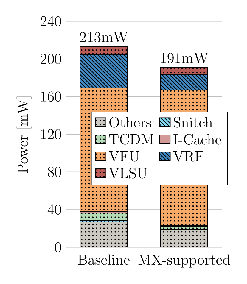
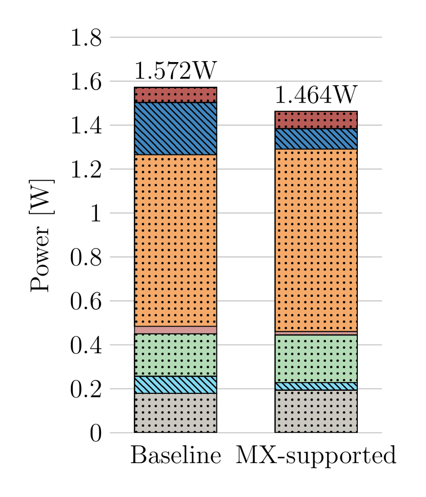
Figure 3: Power breakdown for Dual-Core (Left) and 64-Core clusters (Right) executing MatMul. Dual-Core: at TT@1GHz, executing non-MX (4 vectors, length 32) and MX-ready algorithms ($m^{\prime}=8,n^{\prime}=4,k^{\prime}=4,B=4$). 64-Core: at TT@910MHz, executing non-MX (8 vectors, length 32) and MX-ready algorithms ($m^{\prime}=8,n^{\prime}=4,k^{\prime}=8,B=8$).

IV-C1 Dual-Core Cluster

The upper part of Table IV summarizes the kernel information, execution performance, and energy efficiency for the Dual-Core cluster when executing a $64$-bit MatMul across various problem sizes and tile/sub-tile configurations, highlighting the rows where the kernel’s tile and sub-tile configurations achieve the best energy efficiency. The MX-ready cluster with a sub-tile size of ($8$, $4$, $4$) achieves performance similar to the best-performing execution on the baseline cluster with efficiency gains by +$10.9\text{\,}\%$ (16x16x16), +$10.3\text{\,}\%$ (32x32x32), and +$5.2\text{\,}\%$ (64x64x64).

We evaluate the baseline algorithm using two different output tile configurations with constant sizes. For small problems (16x16x16), the output tile size of $(8,16,1)$ yields higher FPU utilization. As discussed in Section II, although ($8$, $16$, $1$) has higher arithmetic intensity and fewer transfers between TCDM and VRF compared to ($4$, $32$, $1$), the latter configuration benefits from a $$2$\times$ increase in SIMD ratio, leading to better performance for larger problem sizes. For the MX-ready algorithm, the output tiles with larger $n$ and equal $n^{\prime}$ sub-tile dimensions consistently yield better performance and energy efficiency. This improvement is attributed to their higher arithmetic intensity and average SIMD ratio. A similar trend is observed for the energy efficiency when increasing the $m^{\prime}$ dimension of the sub-tile. Due to the higher arithmetic intensity, the power decreases when the output tile size changes from ($4$, $16$, $4$) to ($8$, $8$, $4$). However, the ($4$, $16$, $4$) configuration achieves higher performance thanks to more and shorter matrix result stores, which can be interleaved with computational instructions to hide latency.

The left part of Figure 3 presents the power breakdown of the Dual-Core cluster’s baseline and MX-ready execution of a 64x64x64 MatMul, with the most energy-efficient tile and sub-tile size in our benchmarks. MX reduces VRF access for the B tile and intermediate result storage, leading to a $53.5\text{\,}\%$ reduction in VRF power consumption. Although the sub-tile buffer integration results in a slight $9.4\text{\,}\%$ power increase in VFU, the overall VPU power decreases by $4.1\text{\,}\%$. We also observed a power decrease across the rest of the cluster components, including the Snitch core, instruction caches, and TCDM. This reduction is attributed to the higher SIMD ratio and tiled memory request pattern in MX-ready execution, which eliminates the multiple requests for scalar operands generated by the Snitch core in the baseline. As a result, the total power savings for the Dual-Core cluster achieved through MX amounts to $10.4\text{\,}\%$.

IV-C2 64-Core Cluster

Our benchmark results for various problem sizes on MemPool${}_{$64$}$Spatz${}_{$4$}$ are presented in the bottom section of Table IV. In such a large interconnected memory, contentions may occur when memory requests in the same tile access the same local bank or the same remote group in the same cycle. This generates stalls of the VLSU and increases the access latency. Although such contentions could be mitigated by allocating data structures in a local tile’s memory [14], this approach is hard to implement for MatMul, which inherently requires an extremely global data access pattern.

MX regular memory accesses alleviate contention and improve VLSU utilization by distributing vector element loads/stores across different banks and groups in a strided fashion, contrasting with the baseline where vector elements are fetched from continuous addresses within the same group by both scalar and vector core. This is even more evident with small matrices, where the initial vector load and final result store constitute a significant portion of the total runtime due to the inability to hide latency. FPU utilization increases from $50.4$% to $78.7$%, leading to a $56$% improvement in cluster performance.

Despite a power consumption increase due to the higher FPU utilization, the MX-ready cluster achieves $25\text{\,}\%$ better energy efficiency. Even though the baseline kernels already achieve near-peak utilization for matrix sizes of 128x128x128 and 256x256x256, with the same arithmetic intensity, MX still improves performance by $5.6\text{\,}\%$ and $2.3\text{\,}\%$, with energy efficiency gains by $13.4\text{\,}\%$ and $9.8\text{\,}\%$, respectively. The right side of Figure 3 presents the MemPool${}_{$64$}$Spatz${}_{$4$}$-related power breakdown comparison for a 256x256x256 MatMul. MX reduces the VRF power consumption by $60\text{\,}\%$, thanks to fewer accesses achieved by buffering intermediate results. The VFU power increases by only $6\text{\,}\%$, which comes from the sub-tile buffer and higher FPU utilization. Overall, MX leads to a $6.9\text{\,}\%$ cluster power reduction with near-peak FPU utilization.

These analyses on both small- and large-scale vector clusters demonstrate that MX significantly improves the energy efficiency by reducing the power consumption related to the VRF accesses. MX also pushes the FPU utilization closer to its peak with a negligible area overhead. A quantitative comparison of MX against [7, 8] is hard since none of them presents area or power results, and the effective MatMul speed-up is unclear [7].

V Conclusion

In this paper, we presented MX, an RVV-based ISA extension to support tiled matrix operations for energy-efficient MatMuls. With an embedded-device-friendly and extremely low footprint overhead, MX enhances the energy efficiency of MatMul by means of a small tile buffer near the FPUs, which minimizes the VRF accesses by storing and reusing both input and output matrix tiles. Moreover, MX reduces the number of instructions fetched by the scalar core, decreases the interaction between the scalar and vector cores, and regularizes the memory access pattern, further reducing power consumption. We characterized MX by implementing it on two multi-core clusters in a modern 12-nm technology node. With less than $3\text{\,}\%$ area overhead and no impact on the operating frequency, MX significantly boosts MatMul’s energy efficiency of a Dual-Core cluster by up to $10.9\text{\,}\%$. In a 64-Core cluster and 64x64 matrices, performance and energy efficiency improve by $56\text{\,}\%$ and $25\text{\,}\%$, respectively, further pushing the FPU utilization toward the theoretical peak.

References

- [1] B. Peccerillo, M. Mannino, A. Mondelli, and S. Bartolini, “A survey on hardware accelerators: Taxonomy, trends, challenges, and perspectives,” Journal of Systems Architecture, vol. 129, p. 102561, 2022.
- [2] H. Amiri and A. Shahbahrami, “Simd programming using Intel vector extensions,” J. of Parallel and Distr. Comp., vol. 135, pp. 83–100, 2020.
- [3] S. Deng, H. Zhao, W. Fang, J. Yin, S. Dustdar, and A. Y. Zomaya, “Edge intelligence: The confluence of edge computing and artificial intelligence,” IEEE Internet of Things Journal, vol. 7, no. 8, pp. 7457–7469, 2020.
- [4] N. Jouppi, C. Young, N. Patil, and D. Patterson, “Motivation for and evaluation of the first tensor processing unit,” IEEE Micro, vol. 38, no. 3, pp. 10–19, 2018.
- [5] C. AI, “Edge TPU performance benchmarks,” 2020. [Online]. Available: https://coral.ai/docs/edgetpu/benchmarks
- [6] Y.-H. Chen, T. Krishna, J. S. Emer, and V. Sze, “Eyeriss: An energy-efficient reconfigurable accelerator for deep convolutional neural networks,” IEEE Journal of Solid-State Circuits, vol. 52, no. 1, pp. 127–138, 2017.
- [7] V. Verma, T. Tracy II, and M. R. Stan, “EXTREM-EDGE - EXtensions To RISC-V for Energy-efficient ML inference at the EDGE of IoT,” Sust. Comp.: Informatics and Systems, vol. 35, p. 100742, 2022.
- [8] T-Head Semiconductor, RISC-V Matrix Multiplication Extension Specification, T-Head Semiconductor, 2023. [Online]. Available: https://github.com/T-head-Semi/riscv-matrix-extension-spec/releases/tag/v0.3.0
- [9] M. Cavalcante, D. Wüthrich, M. Perotti, S. Riedel, and L. Benini, “Spatz: A compact vector processing unit for high-performance and energy-efficient shared-L1 clusters,” in Proc. of the 41st ICCAD. San Diego, CA, USA: IEEE/ACM, Oct. 2022.
- [10] H. T. Kung, “Memory requirements for balanced computer architectures,” SIGARCH Comp. Arch. News, vol. 14, no. 2, p. 49–54, May 1986.
- [11] B. Dally, “Hardware for deep learning,” in Hot Chips, Stanford, CA, USA, Aug. 2023.
- [12] M. Perotti, M. Cavalcante, N. Wistoff, R. Andri, L. Cavigelli, and L. Benini, “A ‘New Ara’ for Vector Computing: an Open Source Highly Efficient RISC-V V 1.0 Vector Processor Design,” in Proceedings of the 33rd IEEE Int. Conf. on ASAP. Gothenburg, Sweden: IEEE, Jul. 2022.
- [13] S. Riedel, M. Cavalcante, R. Andri, and L. Benini, “MemPool: A scalable manycore architecture with a low-latency shared L1 memory,” IEEE Transactions on Computers, 2023, early access.
- [14] M. Bertuletti, Y. Zhang, A. Vanelli-Coralli, and L. Benini, “Efficient parallelization of 5G-PUSCH on a scalable RISC-V many-core processor,” in Proc. of the 2023 DATE Conf. Antwerp, Belgium: IEEE, Mar. 2023.