Task-Oriented Active Learning of Model Preconditions
for Inaccurate Dynamics Models

Abstract

When planning with an inaccurate dynamics model, a practical strategy is to restrict planning to regions of state-action space where the model is accurate: also known as a model precondition. Empirical real-world trajectory data is valuable for defining data-driven model preconditions regardless of the model form (analytical, simulator, learned, etc…). However, real-world data is often expensive and dangerous to collect. In order to achieve data efficiency, this paper presents an algorithm for actively selecting trajectories to learn a model precondition for an inaccurate pre-specified dynamics model. Our proposed techniques address challenges arising from the sequential nature of trajectories, and potential benefit of prioritizing task-relevant data. The experimental analysis shows how algorithmic properties affect performance in three planning scenarios: icy gridworld, simulated plant watering, and real-world plant watering. Results demonstrate an improvement of approximately 80% after only four real-world trajectories when using our proposed techniques. More material can be found on our project website: https://sites.google.com/view/active-mde.

I Introduction

Many planning and control frameworks used in robotics rely on dynamics models, whether analytical or learned, to reason about how the robot’s actions affect the state of the environment [1, 2]. However, robots deployed in the real world frequently encounter unstructured environments and complex interactions, e.g., with deformable objects, where assumptions of simplified dynamics break, making the models deviate from reality. In such situations, previous works [3, 4, 5, 6] show how predicting model deviation with a Model Deviation Estimator (MDE) can be a powerful tool to restrict model-based planners to planning in regions of state-action space where the model is reliable, which we call model preconditions. Although using model preconditions defined by MDEs can improve the reliability of plans computed with inaccurate models, training MDEs requires real-world data, which can be expensive or dangerous, e.g., robot welding or pouring water, and drastically increase the cost of exploration during training.

We illustrate the intuition of our problem setting and approach in Fig. 1. Given a dynamics model that is accurate in only some combinations of states and actions, the objective is to estimate model deviation in state-action space to define the model precondition. During each iteration, the robot collects data and updates its model precondition based on that data, which is a form of active learning. Although we can draw from existing active learning techniques in other robotics applications [7], collecting a useful MDE dataset is challenging because it needs to contain a diverse set of trajectories to both identify the limits of the model and reliably solve planning problems. Furthermore, model error in earlier states of a selected trajectory can lead the robot to be unable to gather data from the later states due to the sequential nature of the problem.

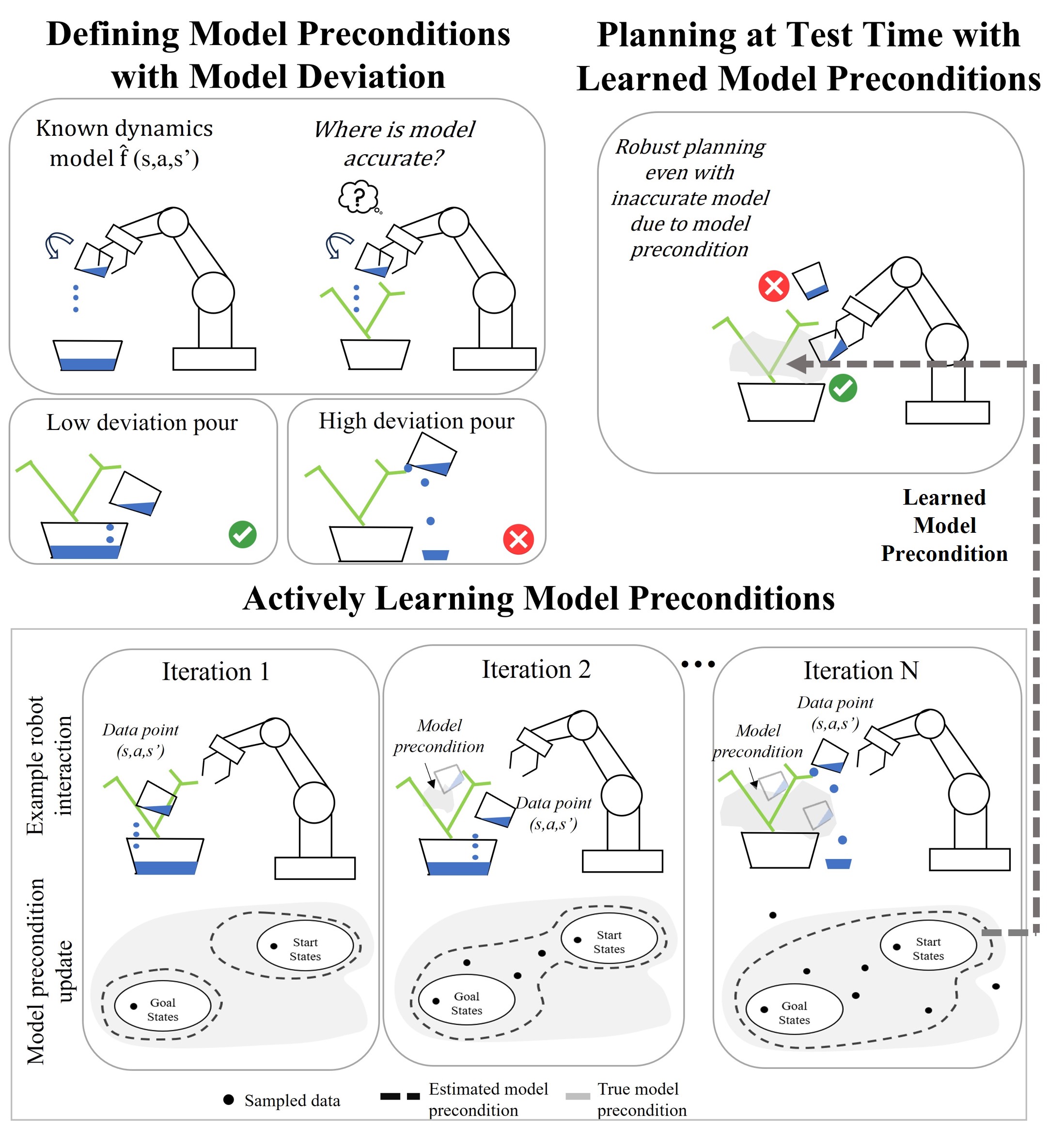
Figure 1: Illustrative example of using a planner and acquisition function to iteratively select informative trajectories to define where the model is accurate to compute plans to the goal. In this example, the known dynamics model on the upper left $(\hat{f}(s,a,s^{\prime}))$ reasons only about the containers but not about the plant. The problem is to define where the model is accurate enough to compute plans to the goal. The resulting learned model precondition is then used at test time to only perform actions in the model precondition.

To address these problems, we describe active learning techniques for efficiently selecting trajectories to train the MDE. We propose a task-oriented approach for generating trajectory candidates, as well as multi-step acquisition functions for selecting the trajectory and methods to compute a single utility value from the sequence of transitions in a trajectory. Our approach enables sample-efficient learning of an MDE for solving tasks from a given distribution. We analyze how variations on the active learning algorithm affect the dataset, and subsequently the quality of the model preconditions when executing plans at test time.

This paper makes the following contributions: (1) a novel problem formulation and approach for active learning of model preconditions defined by MDEs to improve the accuracy and robustness of plans for manipulation task with variable-accuracy models; (2) analysis of the effect of several different acquisition functions on trajectory selection during training and the resulting reliability of the plans executed at test time.

II Problem Statement

In this work, we actively learn model preconditions for planning with inaccurate dynamics models of the form $\hat{s}\leftarrow\hat{f}(s,a)$. We do not make additional assumptions on the implementation or source of the model (e.g. analytical model, simulator, learned model). A model precondition, denoted as $\mathrm{pre}(\hat{f})$, is a region for a given dynamics model where a planner may use $\hat{f}(s,a)$ to compute plans.

The planning problems in our setting are defined by sampling a start state and goal function $g(s)$ that outputs whether or not $s$ is a goal state. Goals are achieved by planning and executing a trajectory defined by actions $a_{1:T-1}$ and predicted states $\hat{s}_{1:T}$ such that $g(s_{T})$ holds. We assume that $\hat{f}(s,a)$ is sufficient for solving the planning problems. At test time, the planner uses the learned model precondition to reject transitions where $(s,a)\notin\mathrm{pre}(\hat{f})$.

The concrete form of model preconditions we use describes $(s,a,s^{\prime})$ transitions where the deviation between predicted states and next states $d(\hat{s},s^{\prime})$ stay within a threshold tolerance, $d_{\mathrm{max}}$, that the system can tolerate or correct. $d(s_{i},s_{j})$ is a distance function, such as Euclidean distance, that outputs a scalar. The constraint can then be defined as $\mathrm{pre}(s,a)=\{s,a\,|\,d(s^{\prime},\hat{f}(s,a))<d_{\mathrm{max}}\}$. Since $d(s^{\prime},\hat{f}(s,a))$ is impossible to compute without knowing $s^{\prime}$, we instead estimate $d(s^{\prime},\hat{f}(s,a))$ given $(s,a)$, denoted as $\hat{d}(s,a)$ to indicate that it is estimated for a state and action.

The active learning problem in this work is to select a set of (variable-length) trajectories to form a dataset $\mathcal{D}$ of $(s,a,s^{\prime})$ tuples on which an MDE is trained. Each trajectory is denoted by $\tau$, and we describe the set of candidate trajectories that different searches generate for the same problem as $\bm{\mathcal{T}}$. The agent may use the planner during training time and sample from the same distribution of planning problems that will be seen at test time, but not the same problems. We assume access to sufficiently accurate state estimation to compute meaningful deviations between all observed points on the trajectory.

III Related Work

Addressing the challenges of planning with inaccurate models is addressed by a variety of techniques such as adaptive control [8, 9], reasoning about uncertainty with probabilistic models [10, 11, 12], and learning dynamics models from data [13, 14, 15].These techniques come with inherent limitations. For instance, probabilistic dynamics models, while designed to mitigate undesirable effects of model deviation, are still susceptible to inaccuracy [16]. Furthermore, certain models, including simulators and many analytical models, lack the capacity to account for uncertainty. Despite these limitations, such models demonstrate practical utility in various planning tasks.

Our approach does not intend to replace learned or uncertain dynamics models, but rather to complement them to address persistent model inaccuracies. Other work has shown that estimating model deviations can be more data-efficient than learning a dynamics model with an equivalent amount of data, and lead to higher reliability when planning with models with limited capacity [4, 17, 3].

Active model precondition learning is similar to active skill precondition learning [18, 7], which also uses GPs to determine which action parameters to sample for successfully executed skills given the state and context. Active dynamics learning [19, 20] can address the additional challenge of sequential dependence of selecting informative points, but these works put strong assumptions on the form of the dynamics model, whereas we extend our scope to allow model preconditions over various types of models such as analytical models and simulators. Model preconditions are different but potentially more generalizable than skill preconditions since multiple model-based behaviours can be use the same model preconditions.

Real-world fluid manipulation particularly benefits from efficient exploration. Existing works tend to be conservative in action space by limiting pours to a small region, such as directly over a target container, which greatly limits the set of observable dynamics  [21, 22, 23]. Furthermore, other approaches are largely constrained to scenarios with simple dynamics [24, 25, 23, 26] where failure tends to be over-pouring or under-pouring. To our knowledge, this is the first experimental setup that uses a commonly-used 7 DOF manipulator to perform actions that often spill water into the workspace.

IV Learning a Model-Deviation Estimator

As defined in Section II, an MDE predicts the deviation $d(\hat{s},s^{\prime})$ for a particular model $\hat{f}(s,a)$ between a predicted state $\hat{s}$ and the true next state $s^{\prime}$. We denote the output of an MDE as $\hat{d}(s,a)$. We implement the MDE in this work using a Gaussian Process (GP) model with a Matérn kernel and heteroscedastic noise model, specifying a Gaussian distribution for the deviation with mean $\mu(\hat{d}(s,a))$ and standard deviation $\sigma(\hat{d}(s,a))$.

Data collected for the MDE is in the form of $(s,a,s^{\prime})$ tuples from executing action $a$ in the target environment (i.e., the real world) from state $s$, and then observing $s^{\prime}$. The input to the MDE is $(s,a)$ and the label is $d(\hat{f}(s,a),s^{\prime})$. A learned MDE then defines a model’s precondition as: $\mathrm{pre}(\hat{f})=\{(s,a)|P(\hat{d}(s,a)>d_{\mathrm{max}})<\delta\}$ for some small probability $\delta$. The constraint can be written as $\mu(s,a)+\beta\sigma(s,a)<d_{\mathrm{max}}$, where the higher $\beta$ is, the lower the risk tolerance. During the training phase, we induce additional exploratory behaviour by setting the prior mean of the GP to zero.

V Active Learning

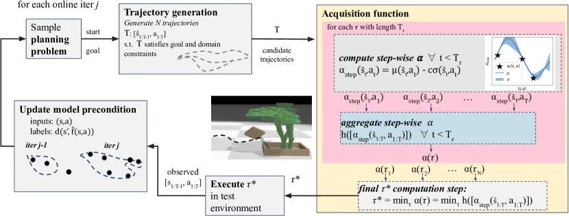
Figure 2: Overview of our method: Each iteration $j$ starts with sampling a planning problem and generating candidate trajectories that satisfy domain constraints and reach the goal. We outline the acquisition function computation for each trajectory in the pink box, including the step-wise acquisition function values, $\alpha_{\mathrm{step}}(s_{t},a_{t})$ for each state-action pair in the trajectory. These values are then aggregated by a function $h$ to yield the trajectory’s utility: $\alpha(\tau)$ . The final step is selecting and executing $\tau*$, in the test environment to collect the ground truth $[s_{[1:T_{\tau}]},a_{[1:T_{\tau}-1]}]$. The MDE is updated every $M$ trajectories.

The algorithm for actively learning MDEs is illustrated in Fig. 2. First, the agent samples a planning problem and then uses a motion planner to generate candidate trajectories. We use a rapidly exploring random tree (RRT) planner [27] to encourage a diverse set of solutions. Then, it selects a trajectory to execute that minimizes an acquisition function $\alpha(\tau)$. After a batch of $M$ executed trajectories, the robot updates the MDE using the observed $(s,a,s^{\prime})$ tuples, ideally expanding the model precondition region between the start and goal states as shown in Fig. 1.

At test time, the robot uses the final model deviation estimator trained on data $\mathcal{D}$ to find plans predicted to be robust using the constraint described in Section II.

V-A Acquisition Function

Now, we explain how we define the acquisition function $\alpha(\tau)$, which guides our selection of the trajectory to execute in each iteration: $\tau^{*}\leftarrow\mathrm{argmin}_{\tau\in\bm{\mathcal{T}}};\alpha(\tau)$. The procedure is illustrated in the rightmost box of Fig. 2.

Step-wise utilities: First, we compute utilities for each step in the trajectory, which is shown in the dotted box. Trajectories can vary in length, denoted as $T_{\tau}$, and are comprised of states and actions: $s_{1:T_{\tau}},a_{1:T_{\tau}-1}$. We denote the utility for each step $t$ as $\alpha_{\mathrm{step}}(s_{t},a_{t})$ and define it using a form inspired by Lower Confidence Bound: $\mu(x)-c\sigma(x)$ where $c$ controls exploration.

Aggregating individual step-wise utilities for a trajectory: As shown in the blue dotted box with $\alpha_{step}(s_{1:T_{\tau}},a_{1:T_{\tau}})$ as inputs, we next define a function $h$ to aggregate a sequence of single-step utilities in trajectories of different lengths,$\alpha_{\mathrm{step}}$, to a single trajectory utility, $\alpha(\tau)$.

The general form of a trajectory-based acquisition function using the lower confidence bound-based $\alpha_{\mathrm{step}}$ is thus:

$$\alpha(\tau)\leftarrow h([\mu(\hat{d}(s_{t},a_{t}))-c\sigma(\hat{d}(s_{t},a_{t}))]\;\forall t<T_{\tau})$$ (1)

To account for the fact that later transitions may not be reached when the trajectory is planned using an inaccurate dynamics model, we introduce $h_{\mathrm{max}}$ and $h_{\mathrm{sum}}$. $h_{\mathrm{max}}=\mathrm{max}_{t<T_{\tau}}\gamma^{t}\alpha_{\mathrm{step}}(s_{t},a_{t})$ and $h_{\mathrm{sum}}=\sum_{t<T_{\tau}}\gamma^{t}\alpha_{\mathrm{step}}(s_{t},a_{t})$. Multiplying each $\alpha_{\mathrm{step}}(s_{t},a_{t})$ by $\gamma^{t}$ approximates the idea that nearer steps are more useful in the trajectory.

V-B Candidate trajectory generation

The effectiveness of the acquisition function depends on the set of candidate trajectories it has to select between.

To set the risk tolerance during training, we propose a schedule for the MDE that gradually reduces risk tolerance as the robot accumulates more data. Since $\delta$ is determined by $\mu(s,a)+\beta\sigma(s,a)$, we can control $\delta$ by modifying $\beta$ using the inverse CDF of a Gaussian distribution: $\beta=\Phi^{-1}(1-\delta)$. At iteration $j$ out of $J$ total iterations, $\beta_{j}\leftarrow\frac{2k_{1}}{1+\mathrm{exp}\bigl{(}-k_{2}(j-\frac{J}{2})\bigr{)}}-k_{1}$ results in a transition from $-k_{1}$ to $k_{1}$ where a lower $k_{2}$ causes a smoother transition.

VI Experimental Setup

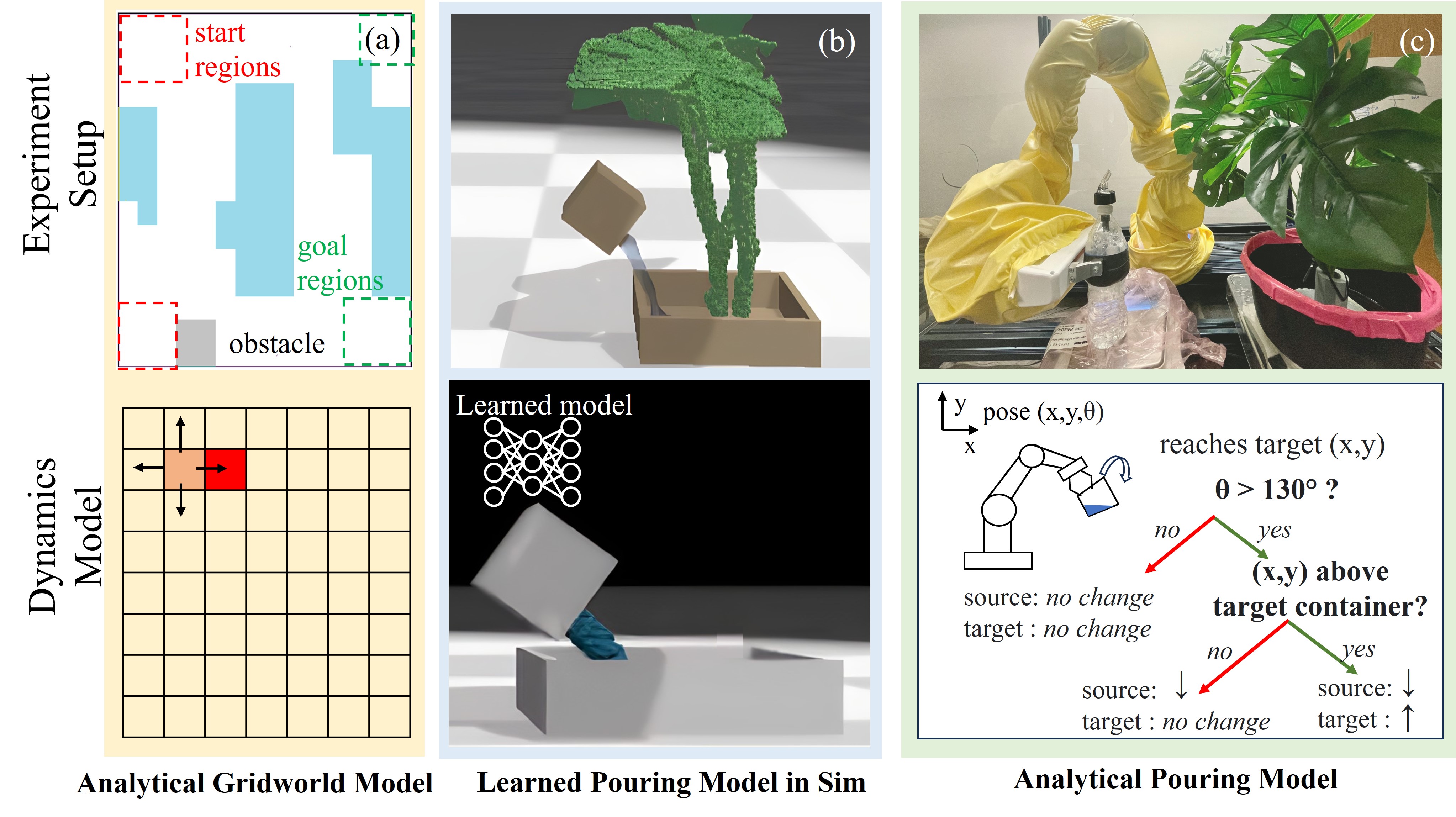
Figure 3: Scenarios and their corresponding dynamics models. (a) slippery grid world where movement may result in slipping backwards over ice (blue) or not moving (grey). The analytical dynamics model assumes unimpeded movement within grid bounds. (b) simulated plant watering using a learned dynamics model trained on a scenario without a plant (c) real-world plant watering with a rule-based analytical dynamics model.

The first scenario, Icy GridWorld (Fig. 3a), is a gridworld also used in [28] where the robot can move in four cardinal directions, but if it moves left or right over an icy state, it slips by moving two cells backwards. The robot cannot move through the obstacle. The dynamics model assumes the robot moves to the intended location. The start and goal state are selected randomly for each planning problem.

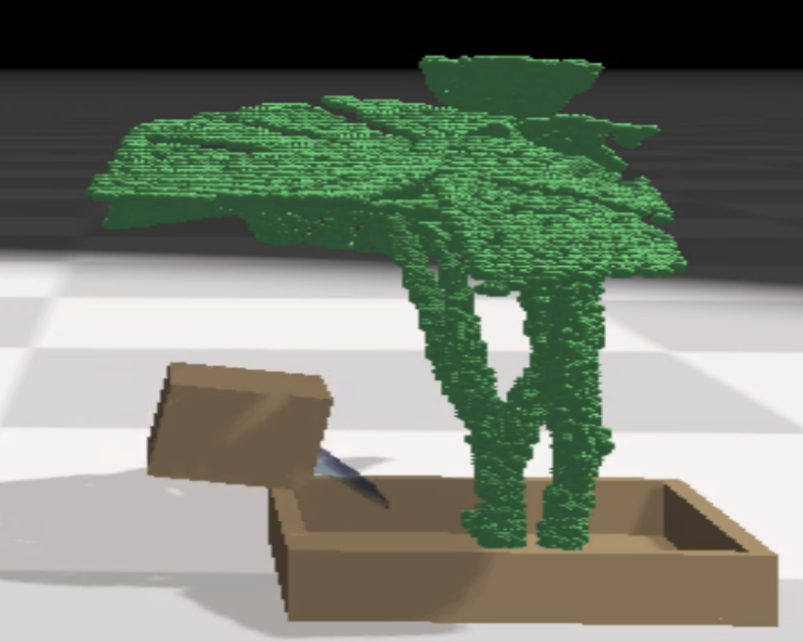
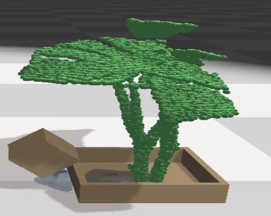
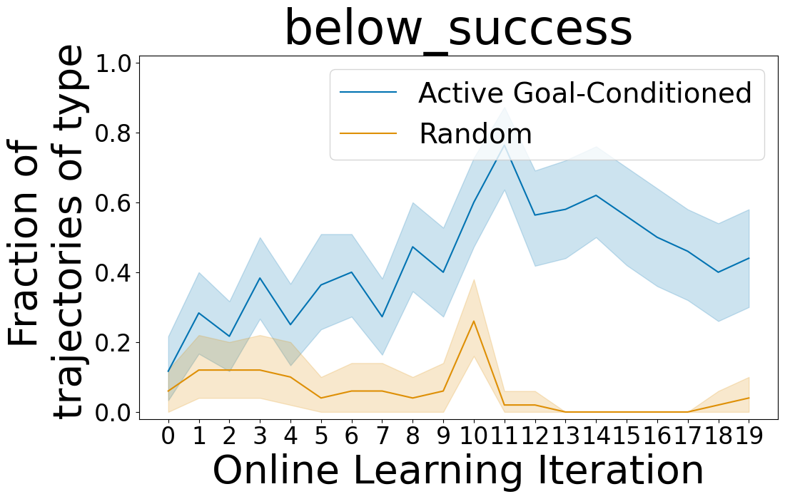
(a) below leaves success

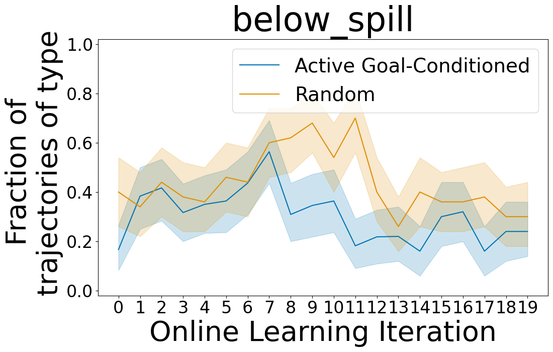
(b) below leaves and spills

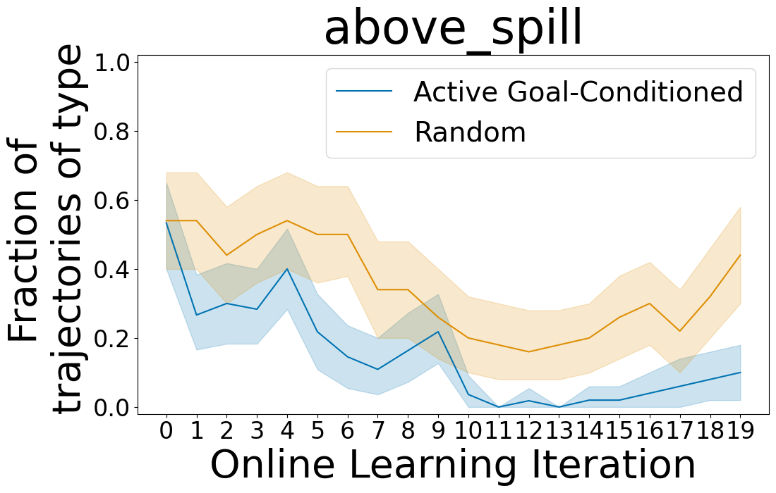
(c) above leaves and spills

Figure 4: Ratio of trajectory types executed during training (examples shown above) for our method and the Random ablation over training iterations.

The second scenario, Water Plant(sim) (Fig. 3b), is a plant-watering domain where the goal is to pour a specified amount of water from a source container into a target container without spilling more than 2%. The state space is the poses of both containers and their liquid volumes. The actions are specified as a target pose for the source container. The actions must satisfy constraints unrelated to the dynamics model including being collision-free according to an approximate collision checker, and either translating or rotating in one motion, but not both. The model is a neural network dynamics model trained in a simpler environment (shown in the bottom half of Fig. 3) with no plant and a wider source container. This scenario tests the algorithm’s ability to learn model preconditions caused by multiple sources of model error such as geometry mismatch, obstruction by leaves, and unexpected collisions. The start state is a random pose left of the target container.

Lastly, the third scenario, Water Plant(real) (Fig. 3c), is a real-world variation of the previous plant-watering domain. A measured pourer dispenses 15 mL of water when tilted above 130 degrees. The action space and state space representations are consistent with the simulated scenario, but we restrict the MDE input to only the desired pose to reduce dimensionality. This scenario demonstrates that reliable performance can be reached in a small number of trajectories (less than a dozen) in the real world where there is considerably more noise and variation. The analytical model we use assumes that 15 mL is dispensed for rotational actions above 130 degrees and that the poured water enters the target container if poured above the area of the container. The start state is fixed and the goal is for 15 mL to be in the target container without spilling more than 5 mL.

Evaluation methodology: On simulated domains, we perform an extensive evaluation on each variation using 10 seeds for 20 learning iterations. Water Plant(sim) uses four training trajectories per iteration, and the others use two per iteration. At test time, we evaluate the model preconditions for each iteration by using the model preconditions where $\hat{d}(s,a)<d_{\mathrm{max}}$ for each transition with 98% confidence. In the simulated scenarios, we sample 20 planning problems per iteration, and in the real-world scenario, we sample 5 per iteration. In Water Plant(real), we only evaluate the effect of using active learning and goal-conditioned candidate trajectories. $d_{\mathrm{max}}=0.1$ for all scenarios and represents the sum of all position distances over all objects. In both watering scenarios, the average volume deviation of both containers is added to the position error. For consistency, we scale the volume units between simulation and the real-world such that one unit is poured out.

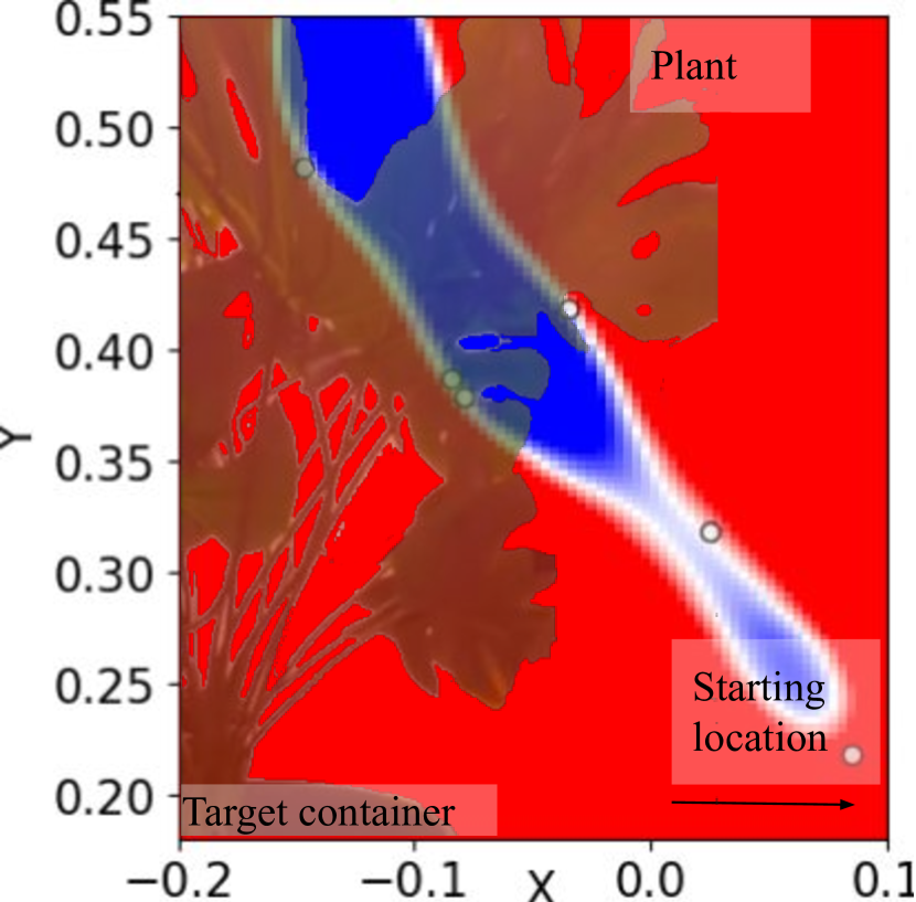
(a) Translation only

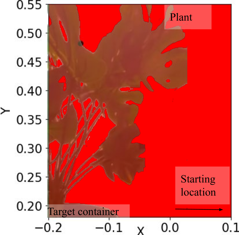
(b) Rotation only

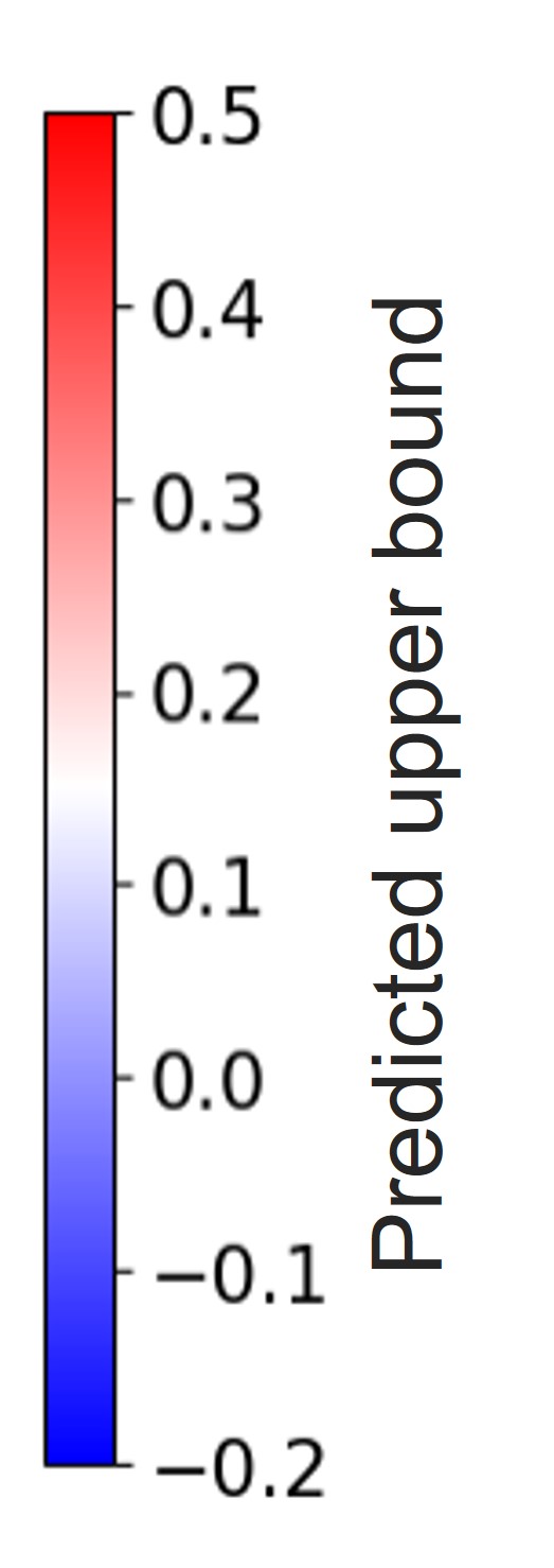
Key

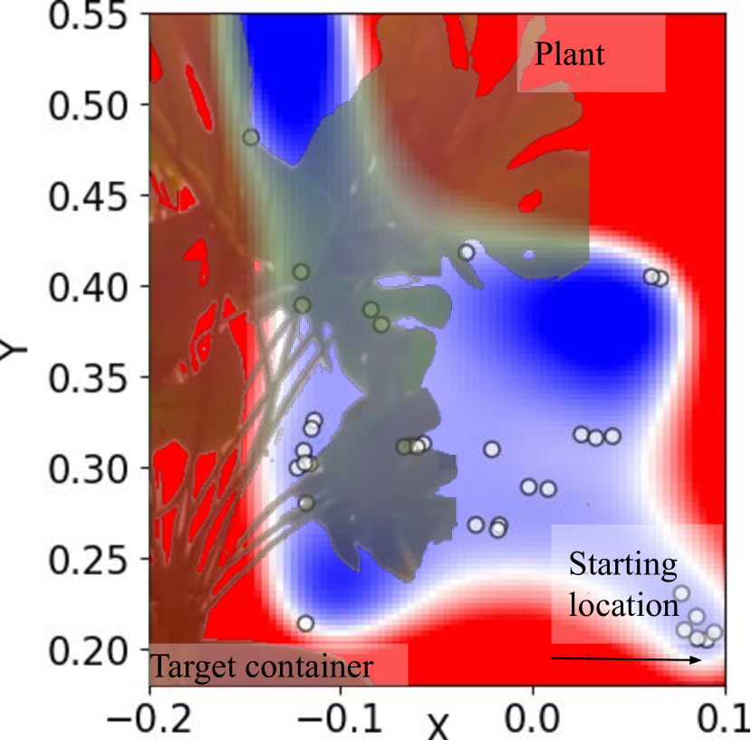
(c) Translation only

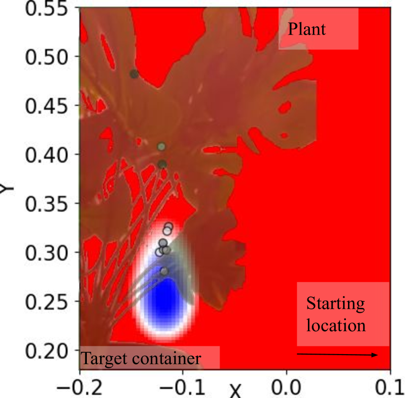
(d) Rotation only

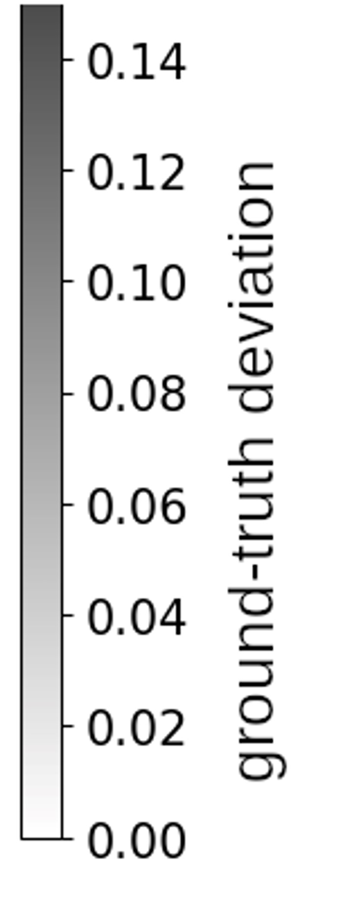
Figure 5: Example MDE with plant overlay over training iterations for translation-only actions and rotation-only actions that can result in pouring. Color scales indicate ground-truth deviation (right, top) and upper bound of the predicted deviation $\mu(\hat{d}(s,a))+\beta\hat{d}(\sigma(s,a))$ for $\beta=2$. $d_{\mathrm{max}}=0.1$, so the blue region indicates the model precondition.

The metrics that we evaluate are as follows. First, we evaluate model precondition accuracy on a cross-validation dataset of trajectories from the other seeds. We measure both the true negative rate (TNR) and the true positive rate (TPR) of whether an individual $(s,a,s^{\prime})$ data point is in the model precondition. A higher rate is better for both metrics, but the TNR is more important than the TPR because the model precondition only needs to cover enough state-action space to compute a plan. Second, we test whether the model precondition is sufficient to reliably compute plans by measuring the success rate of the planner within a fixed timeout of 5000 extensions. Finally, we evaluate the end-to-end success rate in achieving the goal, which measures the effect of using the estimated model preconditions over the entire trajectory.

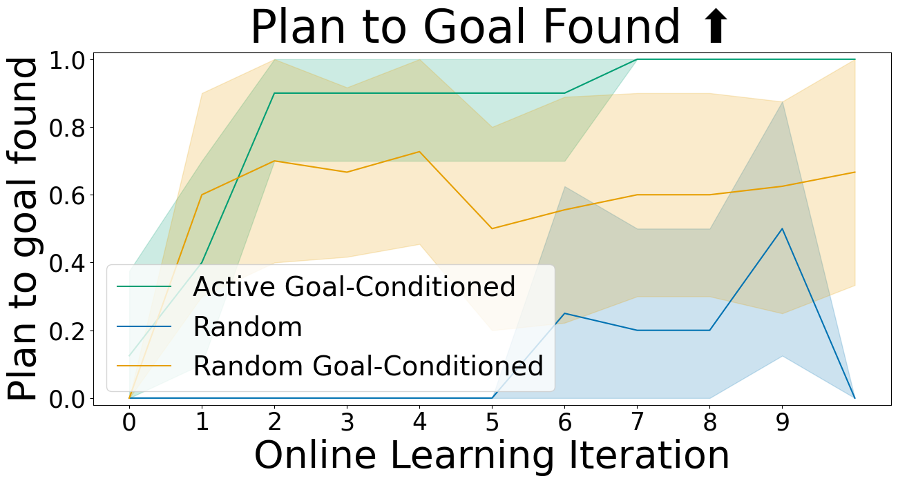
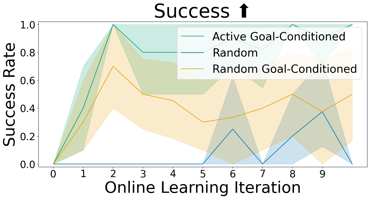
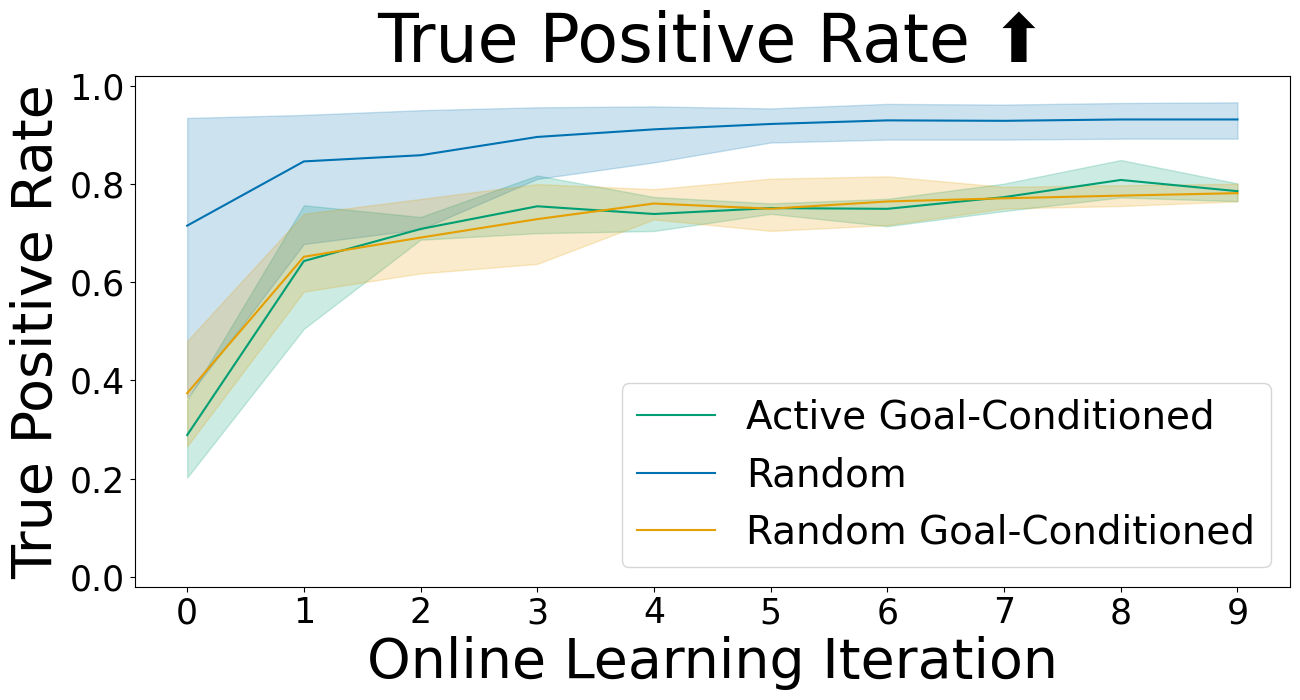
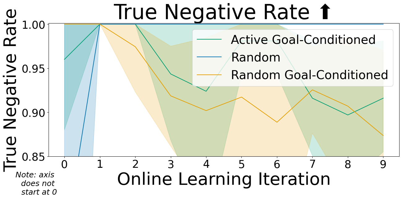
(a) Water Plant(real)

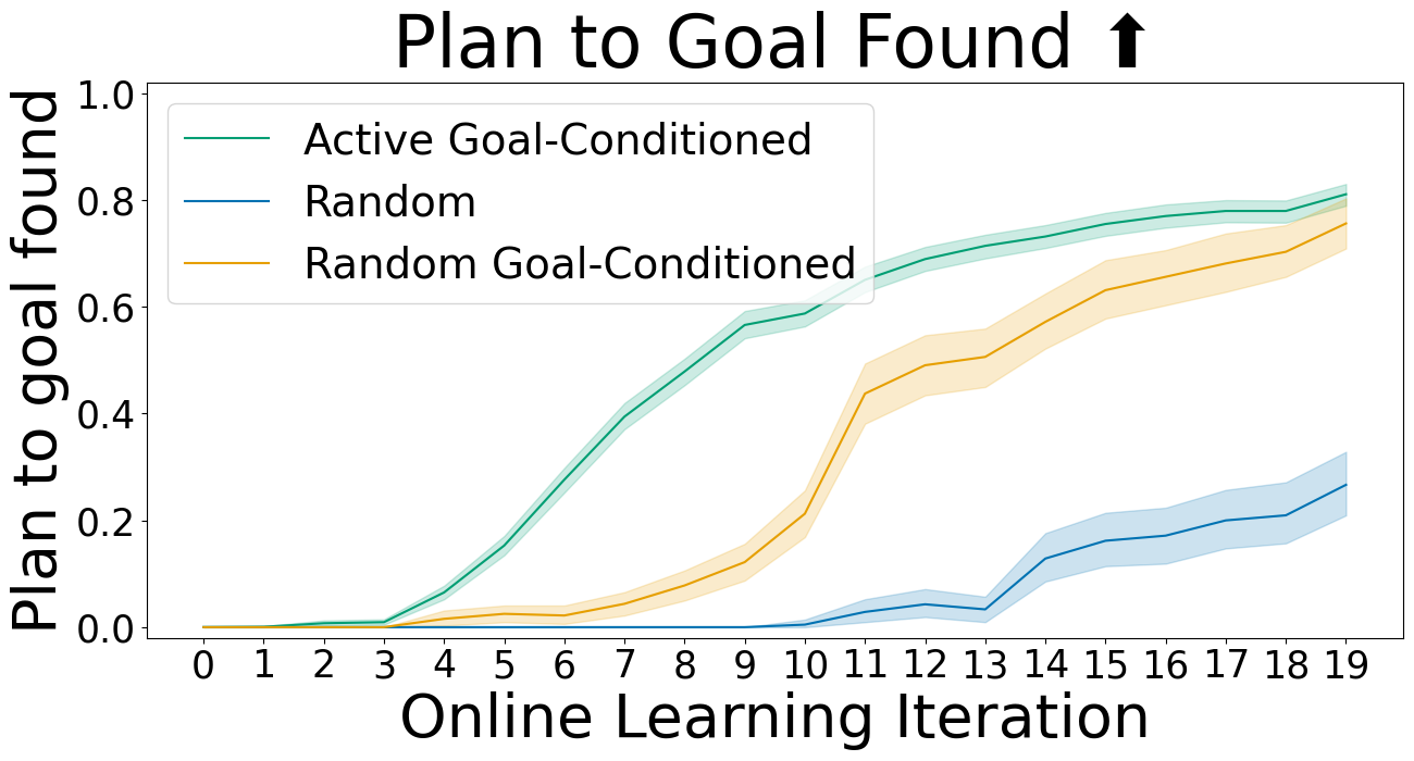
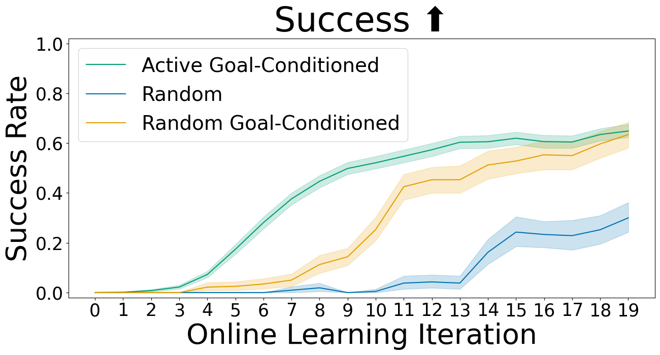
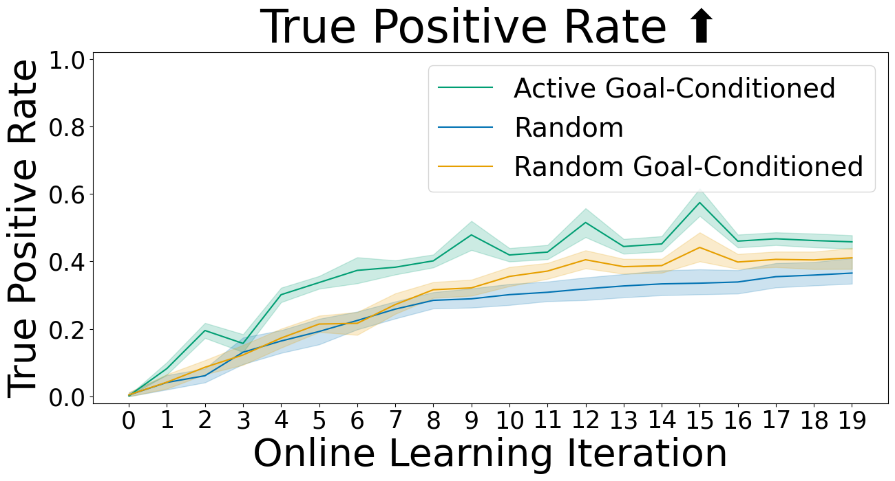
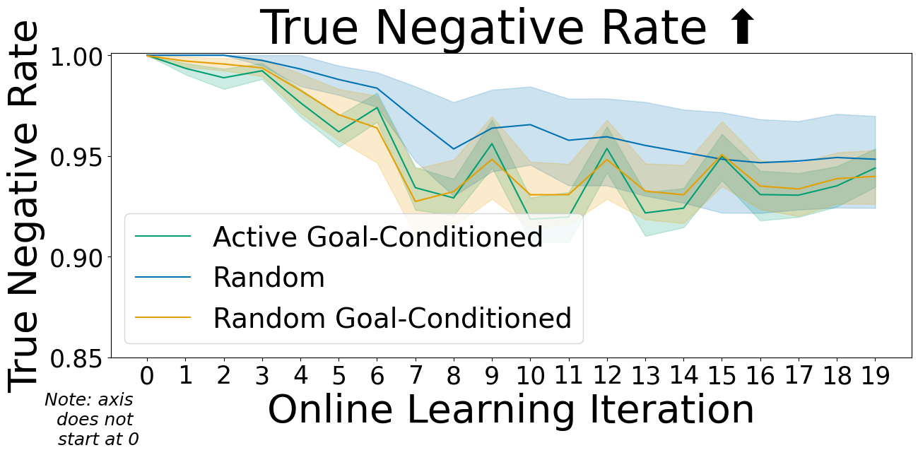
(b) Water Plant(sim)

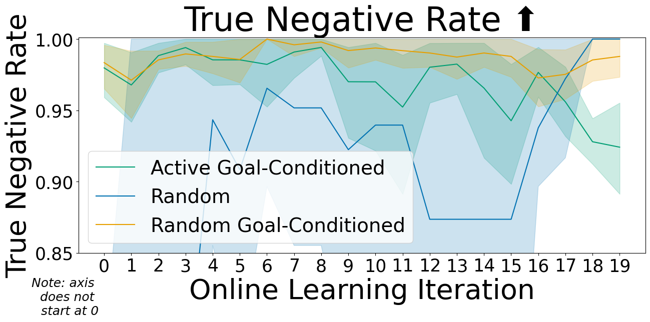
(c) Icy GridWorld

Figure 7: Success rate in computing a plan, success rate in reaching the goal, and model precondition accuracy over training iterations for three scenarios. These plots measure the effect of whether trajectories are selected actively, goal conditioned, or not goal conditioned on performance.

VII Results

We first show a qualitative analysis of the active learning to gain insights into the underlying characteristics of the algorithm. We then quantitatively evaluate the effects of different algorithmic variations using the metrics we previously described in Section VI.

Online learning analysis: Here, we analyze the qualities of the MDE dataset when using our active learning approach described in Section V (Active Goal-Conditioned) compared to selecting trajectories that do not reach the goal, but use the same samplers from the planner, which we call Random. The first row of Fig. 4 shows labels of trajectories selected during training to analyze the makeup of the MDE dataset. below_success is the label for pours below the leaves where all the water reaches the target, which is what would ideally be well represented in the dataset. Since data where the model is inaccurate is also necessary to quantify the limitations of the model, we also track the portion of the dataset that is below_spill. The final trajectory type we track is above_spill, which is the least useful because the water-container-leaf dynamics are typically high-deviation and unnecessary to complete tasks.

Fig. 4 shows a much faster increase in desirable below_success pours from Active Goal-Conditioned in iterations 0 to 9. We note that there is an increase in successful pours around iterations 10-12, which then decreases. As we show in the included video, this effect can be attributed to responses in both aleatoric and epistemic uncertainty, which affects the exploration bonus: $c\sigma(\hat{d}(s,a))$.

Model preconditions in Water Plant(real): Here, we visually analyze how regions of model preconditions change in the real-world pouring task. These regions are low dimensional so it can be visualized in 2D by splitting $\theta_{d}$ into two-cases: one for rotation-only actions, and one for translation-only actions. We show the model precondition by plotting $\hat{d}(s,a)$ over a region of $\mathcal{A}$ (Fig. 5). Aligned with our intuition of how model preconditions should evolve, the area of the model precondition expands as more data is collected. The boundary becomes more precise with more data points (Fig. 5). By iteration 5, the model precondition for rotational actions is in a region above the target container but below the leaves. Note that despite a low-deviation point at iteration 5 at (-0.12, 0.39), that area is not in the model precondition because there is a nearby point that is high-deviation.

VII-A Candidate Trajectory Set Generation

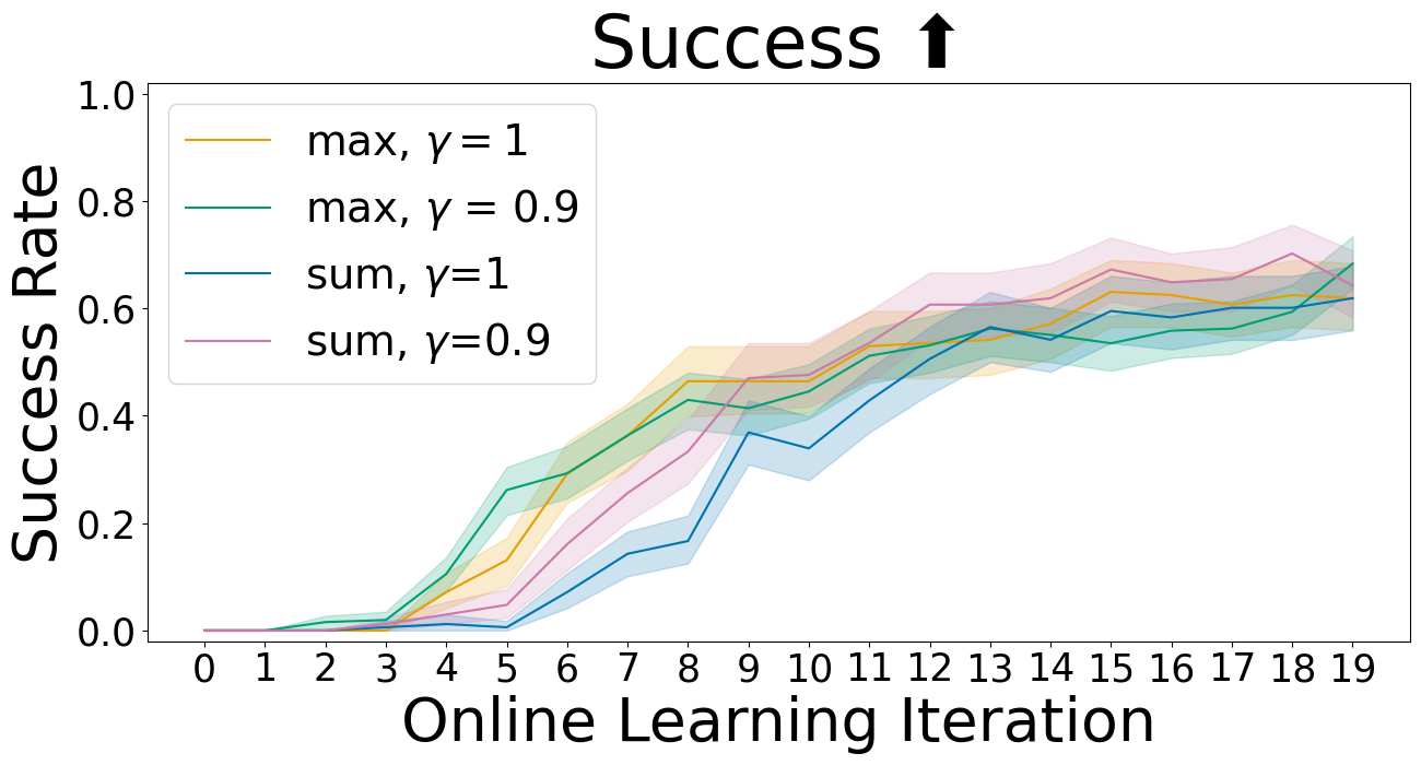
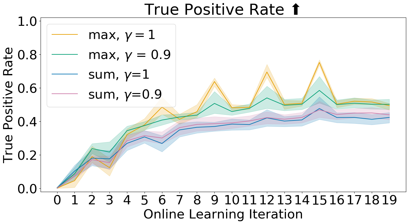
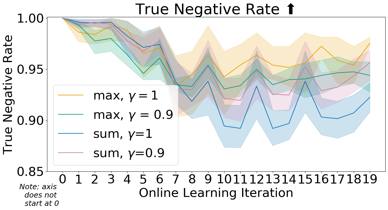
(a) Water Plant(sim)

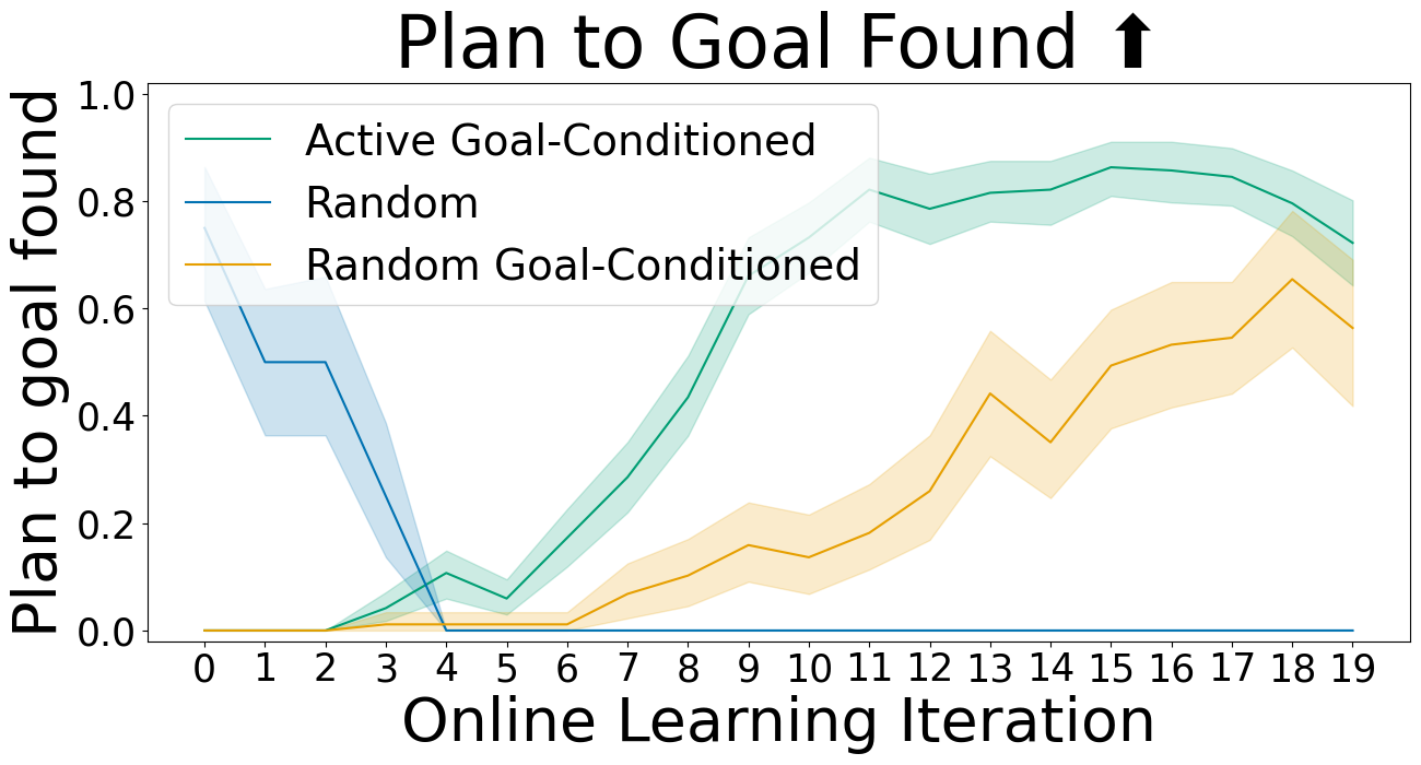
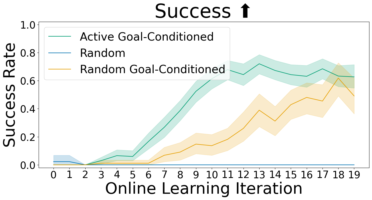
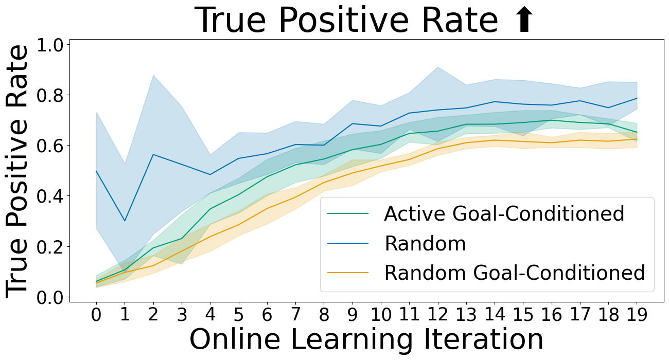
(b) Icy GridWorld

Figure 9: Success rate in computing a plan, success rate in reaching the goal, and model precondition accuracy over training iterations for three scenarios. These plots measure the effect of the aggregation function on performance.

We evaluate how different methods to generate $\bm{\mathcal{T}}$ affects performance metrics. We evaluate the impact of the acquisition function used in Active Goal-Conditioned over an ablation, Goal-Conditioned, that selects a trajectory to the goal randomly.

As shown in Fig. 7, we observe higher data efficiency when using Active Goal-Conditioned or Goal-Conditioned in all scenarios. In Water Plant(sim), we also see significantly higher data efficiency when using active learning in addition to conditioning on trajectories that reach the goal, indicated by higher performance after fewer iterations when using Active Goal-Conditioned over using Goal-Conditioned, which does not use the acquisition function. In Water Plant(real), we see a clear improvement when using goal-conditioning, and a modest improvement in success when using the acquisition function in later iterations. The improvement of Active Goal-Conditioned over Goal-Conditioned in finding plans to the goals is matched by a significant increase in the TPR, which is more significant in the simulated environments than in Water Plant(real). Active Goal-Conditioned shows an improvement in success rate reflected by a higher TNR. Earlier iterations in Icy GridWorld using Random have overly broad model preconditions, as seen by a high TPR, high success in finding goals, but low success in reaching them. Overall, we see a positive affect when using both goal-conditioning and our active learning method.

Notably, accuracy in identifying model preconditions is not necessarily indicative of high performance. As shown in the first row of Fig. 7, although Random has both a high TNR and high TPR, it never finds plans to the goal because of insufficient task-relevant data.

At test time, we observe minor differences in the risk-tolerance schedule by changing $\beta$, where slightly better results are observed when using a fixed $\delta$. We do observe some improvement in data-efficiency when intentionally adding more diversity to the candidate trajectories. Additional results for candidate trajectory generation methods can be found on our website.

VII-B Effect of acquisition function on performance

We analyze the impact of the aggregation function and discount factor on performance. We test $\gamma=0.9$ and compare to no discounting with $\gamma=1$. We observe an slight improvement in performance in both Icy GridWorld and Water Plant(sim) when using $\gamma=0.9$ and $h_{\mathrm{max}}$, which is consistent with our intuition that discounting can account for the dependence of later states on reaching earlier states. The improvement is smaller for Icy GridWorld and more apparent in the success rate in finding plans. Overall, we find that the choice of $\gamma$ and $h$ does not have a major impact on algorithmic performance, but there may be some benefit in using a discount factor, and exploring other forms of aggregation that account for metrics over all the step-wise acquisition function values.

VIII Conclusions

This paper formulates the problem of active learning of model preconditions then presents a novel class of techniques designed to generate and select candidate trajectories. We evaluate the performance of variations on our active learning approach on two simulated scenarios and one real-world task with learned models and analytical models. Our experimental results demonstrate the effect of algorithmic choices in candidate trajectory selection and acquisition function on data efficiency. This work enables empirical estimation of model preconditions with minimal data, a capability we plan to extend to high-dimensional deformable object scenarios where the use of model preconditions can be particularly beneficial.

References

- [1] C. J. Bates, I. Yildirim, J. B. Tenenbaum, and P. Battaglia, “Modeling human intuitions about liquid flow with particle-based simulation,” PLoS computational biology, vol. 15, no. 7, p. e1007210, 2019.
- [2] T. Pfaff, M. Fortunato, A. Sanchez-Gonzalez, and P. Battaglia, “Learning mesh-based simulation with graph networks,” in International Conference on Learning Representations, 2020.
- [3] P. Mitrano, D. McConachie, and D. Berenson, “Learning Where to Trust Unreliable Models in an Unstructured World for Deformable Object Manipulation,” Science Robotics, 2021.
- [4] D. McConachie, T. Power, P. Mitrano, and D. Berenson, “Learning When to Trust a Dynamics Model for Planning in Reduced State Spaces,” IEEE Robotics and Automation Letters, 2020.
- [5] T. Power and D. Berenson, “Keep it simple: Data-efficient learning for controlling complex systems with simple models,” IEEE Robotics and Automation Letters, vol. 6, no. 2, pp. 1184–1191, 2021.
- [6] A. L. LaGrassa and O. Kroemer, “Learning model preconditions for planning with multiple models,” in Conference on Robot Learning, pp. 491–500, PMLR, 2021.
- [7] Z. Wang, C. R. Garrett, L. P. Kaelbling, and T. Lozano-Pérez, “Learning compositional models of robot skills for task and motion planning,” The International Journal of Robotics Research, vol. 40, no. 6-7, pp. 866–894, 2021.
- [8] K. S. Narendra and J. Balakrishnan, “Adaptive control using multiple models,” IEEE transactions on automatic control, vol. 42, no. 2, pp. 171–187, 1997.
- [9] J. Fu, S. Levine, and P. Abbeel, “One-shot learning of manipulation skills with online dynamics adaptation and neural network priors,” in 2016 IEEE/RSJ International Conference on Intelligent Robots and Systems (IROS), pp. 4019–4026, IEEE, 2016.
- [10] E. Páll, A. Sieverling, and O. Brock, “Contingent contact-based motion planning,” in 2018 IEEE/RSJ International Conference on Intelligent Robots and Systems (IROS), pp. 6615–6621, IEEE, 2018.
- [11] L. P. Kaelbling and T. Lozano-Pérez, “Integrated task and motion planning in belief space,” The International Journal of Robotics Research, vol. 32, no. 9-10, pp. 1194–1227, 2013.
- [12] S. Levine and P. Abbeel, “Learning neural network policies with guided policy search under unknown dynamics,” Advances in neural information processing systems, vol. 27, 2014.
- [13] R. Takano, H. Oyama, and Y. Taya, “Robot skill learning with identification of preconditions and postconditions via level set estimation,” in 2022 IEEE/RSJ International Conference on Intelligent Robots and Systems (IROS), pp. 10943–10950, 2022.
- [14] A. Nagabandi, K. Konolige, S. Levine, and V. Kumar, “Deep dynamics models for learning dexterous manipulation,” in Conference on Robot Learning, pp. 1101–1112, PMLR, 2020.
- [15] D. Hafner, T. Lillicrap, I. Fischer, R. Villegas, D. Ha, H. Lee, and J. Davidson, “Learning latent dynamics for planning from pixels,” in International conference on machine learning, pp. 2555–2565, PMLR, 2019.
- [16] C. Guo, G. Pleiss, Y. Sun, and K. Q. Weinberger, “On calibration of modern neural networks,” in International conference on machine learning, pp. 1321–1330, PMLR, 2017.
- [17] H. Liu and G. M. Coghill, “A model-based approach to robot fault diagnosis,” in Applications and Innovations in Intelligent Systems XII: Proceedings of AI-2004, the Twenty-fourth SGAI International Conference on Innovative Techniques and Applications of Artificial Intelligence, pp. 137–150, Springer, 2005.
- [18] Z. Wang, C. R. Garrett, L. P. Kaelbling, and T. Lozano-Pérez, “Active Model Learning and Diverse Action Sampling for Task and Motion Planning,” in 2018 IEEE/RSJ International Conference on Intelligent Robots and Systems (IROS), pp. 4107–4114, Oct. 2018. ISSN: 2153-0866.
- [19] A. Capone, G. Noske, J. Umlauft, T. Beckers, A. Lederer, and S. Hirche, “Localized active learning of gaussian process state space models,” in Learning for Dynamics and Control, pp. 490–499, PMLR, 2020.
- [20] M. Buisson-Fenet, F. Solowjow, and S. Trimpe, “Actively learning gaussian process dynamics,” in Learning for dynamics and control, pp. 5–15, PMLR, 2020.
- [21] N. Correll, N. Arechiga, A. Bolger, M. Bollini, B. Charrow, A. Clayton, F. Dominguez, K. Donahue, S. Dyar, L. Johnson, et al., “Indoor robot gardening: design and implementation,” Intelligent Service Robotics, vol. 3, pp. 219–232, 2010.
- [22] J. Stückler and S. Behnke, “Adaptive tool-use strategies for anthropomorphic service robots,” in 2014 IEEE-RAS International Conference on Humanoid Robots, pp. 755–760, 2014.
- [23] C. Schenck and D. Fox, “Visual closed-loop control for pouring liquids,” in 2017 IEEE International Conference on Robotics and Automation (ICRA), pp. 2629–2636, IEEE, 2017.
- [24] M. Kennedy, K. Schmeckpeper, D. Thakur, C. Jiang, V. Kumar, and K. Daniilidis, “Autonomous precision pouring from unknown containers,” IEEE Robotics and Automation Letters, vol. 4, no. 3, pp. 2317–2324, 2019.
- [25] Y. Noda and K. Terashima, “Modeling and feedforward flow rate control of automatic pouring system with real ladle,” Journal of Robotics and Mechatronics, vol. 19, no. 2, pp. 205–211, 2007.
- [26] J. C. Vaz and P. Oh, “Model-based suppression control for liquid vessels carried by a humanoid robot while stair-climbing,” in 2020 IEEE 16th International Conference on Automation Science and Engineering (CASE), pp. 1540–1545, IEEE, 2020.
- [27] S. LaValle, “Rapidly-exploring random trees: A new tool for path planning,” Research Report 9811, 1998.
- [28] A. Vemula, Y. Oza, J. A. Bagnell, and M. Likhachev, “Planning and execution using inaccurate models with provable guarantees,” in Robotics: Science and Systems XVI, Virtual Event / Corvalis, Oregon, USA, July 12-16, 2020 (M. Toussaint, A. Bicchi, and T. Hermans, eds.), 2020.