Simultaneous Task Allocation and Planning for Multi-Robots
under Hierarchical Temporal Logic Specifications

Abstract

Past research into robotic planning with temporal logic specifications, notably Linear Temporal Logic (LTL), was largely based on singular formulas for individual or groups of robots. But with increasing task complexity, LTL formulas unavoidably grow lengthy, complicating interpretation and specification generation, and straining the computational capacities of the planners. By leveraging the intrinsic structure of tasks, we introduced a hierarchical structure to LTL specifications with requirements on syntax and semantics, and proved that they are more expressive than their flat counterparts. Second, we employ a search-based approach to synthesize plans for a multi-robot system, accomplishing simultaneous task allocation and planning. The search space is approximated by loosely interconnected sub-spaces, with each sub-space corresponding to one LTL specification. The search is predominantly confined to a single sub-space, transitioning to another sub-space under certain conditions, determined by the decomposition of automatons. Moreover, multiple heuristics are formulated to expedite the search significantly. A theoretical analysis concerning completeness and optimality is conducted under mild assumptions. When compared with existing methods on service tasks, our method outperforms in terms of execution times with comparable solution quality. Finally, scalability is evaluated by testing a group of 30 robots and achieving reasonable runtimes.

I Introduction

In the field of multi-robot systems, two primary challenges are consistently at the forefront of research interest: (1) task allocation [1], determining which robot should perform which task, and (2) planning [2], the strategy for executing these assigned tasks. Traditionally, these problems have been tackled separately by researchers from various fields. To simplify these complex issues, certain assumptions or simplifications are often employed, such as the assumption of effective low-level controllers for task allocation or the use of pre-defined tasks in motion planning. These approaches, however, address only portions of the whole problem. Over the past two decades, numerous methods have emerged that address these issues by combining task allocation and motion planning. Our work aligns with this integrative approach, but distinguishes itself by focusing on tasks defined by temporal logic specifications.

Formal methods, characterized by their mathematical rigor, are essential for specifying, developing, analyzing, and verifying software and hardware systems [3]. The recent trend of utilizing formal specifications, such as Linear Temporal Logic (LTL) [4] and Signal Temporal Logic (STL) [5], as high-level task specifications for multi-robots has garnered significant attention. This is because temporal logic specifications can encapsulate not just conventional point-to-point Boolean goals but also complex temporal requirements. While offering an expressive framework for task descriptions, temporal logic specifications also introduce computational challenges for solvers due to their complexity. Take LTL for an example, which is also the formal language we focus on in this work. A typical method for tackling these specifications involves translating the formula into an automaton, a graphic representation. As demonstrated in [6], converting a specification into an automaton that involves the tasks of collecting 5 keys and subsequently opening of 5 doors took about half an hour. A similar problem was observed in our simulations, where an automaton could not be generated within an hour. This issue stems from the usage of the “flat” form of LTL, that is, putting all requirements on the behavior of robots into a single LTL formula. These flat formulas tend to become cumbersome and difficult to interpret for complex tasks. However, one key observation is that in robotics, tasks often have a loose connection and can be broken down into smaller components. Studies also suggest that humans prefer hierarchical task specification, which improves interpretability of planning and execution, making it easier to identify ongoing work and conveniently adjust unfeasible parts without affecting other components [7, 8]. Inspired by this, we propose a hierarchical form of LTL specifications for task specification, along with a planning algorithm.

Consider a mobile manipulation task where multiple robots are tasked with picking and placing three items $a,b$ and $c$ in any order. The “flat” specifications is

$$\phi\,=\, \Diamond(a_{1}\wedge\Diamond a_{2})\wedge\Diamond(b_{1}\wedge\Diamond b_{2})\wedge\Diamond(c_{1}\wedge\Diamond c_{2}),$$

where sub-formula $\Diamond(x_{1}\wedge\Diamond x_{2})$ denotes the event of first picking item $x$ somewhere and then placing it somewhere else. Note that this formula does not explicitly state which robot should pick and place which item. Nevertheless, this formula is less interpretable by users by arranging all sub-formulas side by side. Furthermore, its corresponding automaton, specifically, Nondeterministic B$\ddot{\text{u}}$chi Automaton (NBA), has 27 states and 216 transitions, which is unexpectedly large for a task of this complexity. We propose to take advantage of the task’s inherent hierarchical structure, that is, manipulating each item in any order. A two-level hierarchical form is

$$L_{1}:\quad \phi\;\,=\Diamond\phi_{1}\wedge\Diamond\phi_{2}\wedge\Diamond\phi_{3}$$

$$L_{2}:\quad \phi_{1}=\Diamond(a_{1}\wedge\Diamond a_{2})$$

$$\phi_{2}=\Diamond(b_{1}\wedge\Diamond b_{2})$$

$$\phi_{3}=\Diamond(c_{1}\wedge\Diamond c_{2}),$$

which has 4 specifications, one per row, and their automatons have 17 states and 45 transitions in total. The hierarchical formalism decomposes a flat LTL formula into a hierarchical structure of multiple formulas, whose syntax and semantics will be detailed in Sec. IV. This representation effectively reduces the length of each individual formula, leading to more manageable automaton sizes and consequently improving interpretability.

In this work, we first establish syntax rules for hierarchical specifications and also provide a framework for semantic interpretation. To this aim, considering the context of multiple specifications, we introduce the concept of state-specification plan, which pairs the state of each robot with a specific specification it seeks to fulfill at a given time. Utilizing this concept, we devise an algorithm to check the satisfaction of a set of hierarchical LTL specifications given a state-specification plan. We have proved that the hierarchical form possesses greater expressiveness compared to the flat form. Next, we propose a planning algorithm with formal guarantees of completeness or optimality under mild assumptions. We draw inspiration from the bottom-up approach of [9], which involves searching within a product graph that combines the environment and task space. This method’s advantage is its ability to simultaneously handle task allocation and planning (STAP), ensuring the feasibility of the plan for each robot. In this respect, our work is also closely related to the field of Task and Motion Planning (TAMP) as discussed in [10], where task and motion planning are seamlessly integrated.

To adapt [9] for hierarchical LTL specifications, we approximate the entire search space as a set of loosely interconnected sub-spaces, each corresponding to an individual LTL specification in the hierarchical LTL specifications. The search process primarily occurs within a single sub-space, with transitions to adjacent sub-spaces happening under specific conditions determined by the decomposition of the automatons. Under certain assumptions regarding the state-specification plan, we demonstrate that our planning algorithm is sound, complete, and optimal. Additionally, we introduce several heuristics to expedite the search process. These include minimizing the loose connections between sub-spaces and leveraging task-level progress to guide the search. Extensive simulations on robot service tasks were conducted to evaluate our methods. Comparisons between our approaches with and without heuristics highlight a balance between computational time and solution quality. When compared with work [9], our method shows significant improvements in computational time. Notably, for complex tasks, Schillinger et al. [9]’s method failed to produce solutions within a one-hour timeout. In scalability tests, our method demonstrated the ability to generate sub-optimal solutions in approximately three minutes for intricate tasks involving up to 30 robots. Note that the flat version of these tasks could not be solved using graph-theoretic methods due to the inability to generate an automaton within a one-hour timeout. For ease of reference, a glossary of key notations is provided in Tab. I.

Contributions The contributions of our work are outlined as follows:

1. We introduce a hierarchical form of LTL along with syntax and semantics, and prove it is more expressive than the flat form;

2. A search-based planning algorithm is developed, facilitating simultaneous task allocation and planning. This planner is, to the best of our knowledge, the first to offer both completeness and optimality for hierarchical LTL specifications;

3. We devise multiple heuristics to expedite the search process;

4. Under mild assumptions, we perform theoretical analyses to validate the completeness and optimality of our approach;

5. We conduct extensive comparative simulations focusing on service tasks to showcase the efficiency and scalability of our proposed method.

II Related Work

II-A Multi-robots Planning under Temporal Logic Specifications

In the existing body of research on optimal control synthesis from LTL specifications, two primary approaches are present in handling LTL tasks for multi-robot systems. One approach, as seen in works [11, 12, 13], involves assigning LTL tasks locally to individual robots within the team. The other approach assigns a global LTL specification to the entire team, which encapsulates the collective behavior of all robots. In scenarios where global LTL specifications are used, these specifications can either explicitly assign tasks to individual robots [14, 15, 16, 17, 18, 19, 20, 21, 22, 23], or the tasks may not be explicitly designated to specific robots [24, 25, 26, 27], similar to our problem in this work.

Note that, apart from the study [28] that was developed concurrently, which investigated hierarchical LTL based on this work, all other relevant research concentrates on using flat LTL specifications to describe the desired behaviors in multi-robot systems. To address the complexity of specifying collective behaviors in multi-robot systems, various extensions of temporal logic have been introduced: Sahin et al. [29] developed Counting Temporal Logic (CTL), a tool designed to express the collective behavior of multiple robots. Djeumou et al. [30], Yan et al. [31] utilized Graph Temporal Logic (GTL) and Swarm Signal Temporal Logic (SwarmSTL) respectively. These logics are particularly effective for specifying swarm characteristics like centroid positioning and density distribution. Leahy et al. [32] introduced Capability Temporal Logic (CaTL) to encapsulate the diverse capabilities of robots.

As temporal logic formulas are used to tackle complex tasks involving multiple robots and intricate workspaces, they inevitably become lengthy and complicated. Some attempts have been made to simplify this, such as merging multiple atomic propositions into one using logical operators [20, 23], or combining multiple sub-formulas into one formula using logical operators [16, 15, 29]. Despite these efforts, we still categorize these as the flat form. Notably, temporal operators, the primary feature distinguishing LTL from propositional logic, only appear on one side, either for the integration of merged propositions or inside the sub-formulas. Previous works [25, 29, 32, 33, 34, 35] have defined propositions involving more than one robot to encapsulate collaborative tasks. In our study, we introduce composite propositions that encompass more than one sub-formula and can be combined using temporal operators.

Global temporal logic specifications that do not explicitly assign tasks to robots generally require decomposition to derive the necessary task allocation. This decomposition can be accomplished in three primary ways: The most common method, utilized in works such as [9, 22, 36, 37, 38, 33, 39], involves decomposing a global specification into multiple tasks, which leverages the transition relations within the automaton, which is the graphical representation of an LTL formula. As demonstrated in [25, 29], the second approach builds on Bounded Model Checking (BMC) methods [40] to create a Boolean Satisfaction or Integer Linear Programming (ILP) model, which simultaneously addresses task allocation and implicit task decomposition in a unified formulation. Another method, proposed by [41], directly interacts with the syntax tree of LTL formulas, which segments the global specification into smaller, more manageable sub-specifications.

The works most closely related to our study are [9, 42, 43, 44, 28]. Schillinger et al. [9, 42] approach STAP by breaking down temporal logic tasks into a series of independent tasks, each of which can be completed by a single robot. Faruq et al. [43] build upon this idea, incorporating environmental uncertainties and potential failures into the planning process. Robinson et al. [44] expand this concept further into a multi-objective setting, integrating various conflicting objectives such as cost and success probability into a Markov Decision Process (MDP). Our work aligns with these studies but also presents key differences: (i) While the aforementioned studies focus on flat LTL specifications, our work considers a hierarchical set of LTL specifications. Our simulations demonstrate that we can resolve tasks which are unsolvable by these earlier methods. (ii) In the mentioned studies, temporally dependent tasks are assigned to single robots, and tasks between robots are independent thus robot can execute their tasks in parallel. In contrast, our approach also assigns tasks with temporal dependencies to different robots, thus robots may depend on others, adding a layer of complexity to the STAP problem. In our another work [28], developed around the same time, we implemented a hierarchical approach that initially focused on task allocation followed by planning. This method, however, was unable to achieve STAP. Additionally, the planning algorithm introduced in [28] does not provide formal assurances of either completeness or optimality.

II-B Task Allocation and Planning

In the realm of multi-robot systems, an important area of study is integrated task assignment and path planning. The primary objective is to create collision-free paths for robots, enabling them to accomplish a variety of reach-avoid tasks pending assignment. This field is often associated with the unlabeled version of multi-agent path planning (MAPF), as discussed by [45]. Various formulations have been proposed, including those by [46, 47, 48, 49, 50], to name a few. Chen et al. [48] focus on simultaneous task assignment and path planning for Multi-agent Pickup and Delivery (MAPD) in warehouse settings, where the goal is to efficiently manage agents transporting packages. Aggarwal et al. [49] tackle the combined challenge of task allocation and path planning, where an operator must assign multiple tasks to each vehicle in a fleet, ensuring collision-free travel and minimizing total travel costs. Ma and Koenig [50] explore this issue for teams of agents, each assigned the same number of targets as there are agents in the team. Our work differs from these studies in several key aspects: (i) We do not assume a predefined set of point-to-point navigation tasks. Instead, tasks, which may include navigation and manipulation, are implicitly defined within the temporal logic specifications. This requires the decomposition of tasks from these specifications. (ii) The presence of logical and temporal constraints between tasks adds complexity to our problem. (iii) In our scenario, a single robot might be assigned multiple tasks, while others might remain stationary. This contrasts with scenarios where each robot is assigned exactly one task in works mentioned above. As a result, improved solutions can be achieved through better allocation as opposed to relying on pre-defined allocations.

Another relevant field is Task and Motion Planning (TAMP), which aims to identify a sequence of symbolic actions and corresponding motion plans. An extensive review of TAMP can be found in [10, 51]. TAMP typically focuses on single-robot scenarios. In this work, we concentrate on multi-robot cases, as the aspect of task allocation is not applicable to a single robot. The primary focus in multi-robot TAMP is on the pick-up and placement of multiple objects by multiple manipulators, with the objective of determining which manipulator should pick up which objects and in what manner. One approach within this category employs search-based methods. This includes Conflict Based Search (CBS) [52], Monte-Carlo Tree Search (MCTS) [53], search in hyper-graphs [54], and search based on satisfiability modulo theories (SMT) solvers [55]. Another approach utilizes optimization-based methods. For example, Toussaint [56] proposed the logic-geometric program (LGP), which integrates continuous motion planning and discrete task specifications into optimization problems. Similarly, Envall et al. [57] implicitly assign actions based on the solution to a nonlinear optimization problem. Our work diverges from multi-robot TAMP in two main ways: (i) While TAMP studies mainly focus on pick-and-place manipulation tasks in tabletop environments, our work extends to longer-horizon tasks that take place throughout an entire office building. (ii) Most TAMP studies do not consider logical or temporal constraints, with only a handful addressing dependency constraints that emerge from handover operations. Our approach incorporates these constraints, adding complexity to task planning and execution.

II-C Hierarchical Task Models

Hierarchical reasoning enhances human understanding of the world [7, 8]. In classical AI planning, researchers have crafted various task models reflecting hierarchical structures by employing procedural domain control knowledge [58]. These models have proven to be superior to flat models in terms of interpretability and efficiency, largely due to the significant reduction in the search space for a plan. Hierarchical Task Network (HTN) [59], a commonly used task model in classical AI, exemplifies this. It presents a hierarchy of tasks, each of which can be executed if it’s primitive, or broken down into finer sub-tasks if it’s complex. The planning process begins with decomposing the initial task network and continues until all compound tasks are decomposed, leading to a solution. The resulting plan comprises a set of primitive tasks applicable to the initial world state. Owing to its expressive capacity, HTN has been implemented in the robotic planning [60]. There are other hierarchical models such as AND/OR graphs [61] and sequential/parallel graphs [62].

Research combining hierarchical task models with LTL includes studies that use LTL to express temporally extended preferences over tasks and sub-tasks in HTN [63], as well as research into the expressive power of HTN in combination with LTL [64]. However, despite the widespread use of hierarchical task models in classical AI planning, it’s intriguing to note the lack of specification hierarchy in temporal logic robotic planning. Our work differs from these studies as we follow an inverse direction; instead of integrating LTL into HTN to express the goal of the planning problem, we incorporate HTN into LTL, allowing for hierarchical structures within multiple LTL formulas, making them more capable of expressing complex tasks than a single flat LTL formula.

Notation	Description	Notation	Description
$\pi$	atomic propositions	$\sigma$	infinite word over the alphabet
$\bigcirc$	next operator	${\mathcal{B}}(\phi)$	NBA of specification $\phi$
$\Diamond$	eventual operator	${\mathcal{Q}}_{\mathcal{B}}$	set of automaton states
$\square$	global operator	${\mathcal{Q}}_{\mathcal{B}}^{0}$	set of initial automaton states
$\mathcal{U}$	until operator	$\Sigma=2^{{\mathcal{A}}{\mathcal{P}}}$	alphabet
$\phi$	specification	$\to_{\mathcal{B}}$	transition relation in ${\mathcal{B}}$
${\mathcal{A}}{\mathcal{P}}$	set of atomic propositions	${\mathcal{Q}}_{\mathcal{B}}^{F}$	set of final automaton states
${\mathcal{T}}(r)$	transition system of robot $r$	$\rho_{\mathcal{B}}$	infinite run
${\mathcal{S}}_{r}$	states of robot $r$	${\mathcal{L}}_{\mathcal{B}}$	accepted language of ${\mathcal{B}}$
$s_{r}^{0}$	initial state of robot $r$	${\mathcal{P}}(r,\phi)$	PBA of robot $r$ and specification $\phi$
$\to_{r}$	transition relation of robot $r$	${\mathcal{Q}}_{\mathcal{P}}$	set of product states
${\mathcal{A}}{\mathcal{P}}_{r}$	atomic proposition of robot $r$	${\mathcal{Q}}_{\mathcal{P}}^{0}$	set of initial product states
$L_{r}$	observation function of robot $r$	$\to_{\mathcal{P}}$	transition relation in ${\mathcal{P}}$
$\phi(k,i)$	$i$-th specification at $k$-th level	${\mathcal{Q}}_{\mathcal{P}}^{F}$	set of final states
${\mathcal{G}}_{h}=({\mathcal{V}}_{h},{\mathcal{E}}_{h})$	specification hierarchy graph	$c_{\mathcal{P}}$	cost function in ${\mathcal{P}}$
$\Phi^{k}$	set of specifications at the $k$-th level	$\tau=\tau^{0}\ldots\tau^{h}$	state-specification plan
$\Phi^{K}$	set of specifications at the lowest level	${\mathcal{D}}_{\mathcal{B}}(\phi)$	decomposition set of specification $\phi$
$\Phi^{acc}$	set of satisfied specifications up to certain time	${\mathcal{P}}(\phi)$	product team model associated with specification $\phi$
$\zeta_{\text{in}}$	in-spec switch transition	${\mathcal{P}}$	hierarchical team models
$\zeta_{\text{inter}}^{1}$	type I inter-spec switch transition	$\zeta_{\text{inter}}^{2}$	type II inter-spec switch transition
$v=(r,\phi,\mathbf{s},\mathbf{q})$	search state	$\Lambda=v_{0}\ldots v_{n}$	search path
$\Lambda^{\prime}=\Lambda_{1}\ldots\Lambda_{l}$	search path after removing all switch states	${\mathcal{R}}_{k}$	active robots of the $k$-th path segment

TABLE I: Summary of notations.

III Preliminaries

Notation: Let $\mathbb{N}$ denote the set of all integers, $[K]=\{1,\ldots,K\}$ denote the set of integers from 1 to $K$ and $|\cdot|$ denote the cardinality of a set.

In this section, we formally describe Linear Temporal Logic (LTL) by presenting its syntax and semantics. Also, we briefly review preliminaries of automata-based LTL model checking.

Linear Temporal Logic [65] is a type of formal logic whose basic ingredients are a set of atomic propositions $\mathcal{AP}$, the boolean operators, conjunction $\wedge$ and negation $\neg$, and temporal operators, next $\bigcirc$ and until $\mathcal{U}$. LTL formulas over $\mathcal{AP}$ abide by the grammar

$$\phi::=\text{true}~{}|~{}\pi~{}|~{}\phi_{1}\wedge\phi_{2}~{}|~{}\neg\phi~{}|~{}\bigcirc\phi~{}|~{}\phi_{1}~{}\mathcal{U}~{}\phi_{2}.$$ (1)

For brevity, we abstain from deriving other Boolean and temporal operators, e.g., disjunction $\vee$, implication $\Rightarrow$, always $\square$, eventually $\lozenge$, which can be found in [65].

An infinite word $\sigma$ over the alphabet $2^{\mathcal{AP}}$ is defined as an infinite sequence $\sigma=\pi^{0}\pi^{1}\ldots\in(2^{\mathcal{AP}})^{\omega}$, where $\omega$ denotes an infinite repetition and $\pi^{k}\in 2^{\mathcal{AP}}$, $\forall k\in\mathbb{N}$. The language $\texttt{Words}(\phi)=\left\{\sigma|\sigma\models\phi\right\}$ is defined as the set of words that satisfy the LTL formula $\phi$, where $\models\subseteq(2^{\mathcal{AP}})^{\omega}\times\phi$ is the satisfaction relation. An LTL formula $\phi$ can be translated into a Nondeterministic B$\ddot{\text{u}}$chi Automaton defined as follows [66]:

Definition III.1 (NBA)

A Nondeterministic B$\ddot{\text{u}}$chi Automaton (NBA) ${\mathcal{B}}$ of an LTL formula $\phi$ over $2^{\mathcal{AP}}$ is defined as a tuple ${\mathcal{B}}(\phi)=\left({\mathcal{Q}}_{{\mathcal{B}}},{\mathcal{Q}}_{{\mathcal{B}}}^{0},\Sigma,\rightarrow_{{\mathcal{B}}},\mathcal{Q}_{\mathcal{B}}^{F}\right)$, where

• ${\mathcal{Q}}_{{\mathcal{B}}}$ is the set of states;

• ${\mathcal{Q}}_{{\mathcal{B}}}^{0}\subseteq{\mathcal{Q}}_{{\mathcal{B}}}$ is a set of initial states;

• $\Sigma=2^{\mathcal{AP}}$ is an alphabet;

• $\rightarrow_{{\mathcal{B}}}\,\subseteq\,{\mathcal{Q}}_{{\mathcal{B}}}\times\Sigma\times{\mathcal{Q}}_{{\mathcal{B}}}$ is the transition relation;

• ${\mathcal{Q}}_{{\mathcal{B}}}^{F}\subseteq{\mathcal{Q}}_{{\mathcal{B}}}$ is a set of accepting/final states.

An infinite run $\rho_{{\mathcal{B}}}$ of ${\mathcal{B}}$ over an infinite word $\sigma=\pi_{0}\pi_{1}\pi_{2}\dots$, $\pi_{k}\in\Sigma=2^{\mathcal{AP}}$, $\forall k\in\mathbb{N}$, is a sequence $\rho_{{\mathcal{B}}}=q_{{\mathcal{B}}}^{0}q_{{\mathcal{B}}}^{1}q_{{\mathcal{B}}}^{2}\dots$ such that $q_{{\mathcal{B}}}^{0}\in{\mathcal{Q}}_{{\mathcal{B}}}^{0}$ and $(q_{{\mathcal{B}}}^{k},\pi_{k},q_{{\mathcal{B}}}^{k+1})\in\rightarrow_{{\mathcal{B}}}$, $\forall k\in\mathbb{N}$. An infinite run $\rho_{{\mathcal{B}}}$ is called accepting if $\texttt{Inf}(\rho_{{\mathcal{B}}})\cap{\mathcal{Q}}_{{\mathcal{B}}}^{F}\neq\varnothing$, where $\texttt{Inf}(\rho_{{\mathcal{B}}})$ represents the set of states that appear in $\rho_{{\mathcal{B}}}$ infinitely often. The words $\sigma$ that produce an accepting run of ${\mathcal{B}}$ constitute the accepted language of ${\mathcal{B}}$, denoted by ${\mathcal{L}}_{{\mathcal{B}}}$. Then Baier and Katoen [65] prove that the accepted language of ${\mathcal{B}}$ is equivalent to the words of $\phi$, i.e., ${\mathcal{L}}_{{\mathcal{B}}}=\texttt{Words}(\phi)$.

The dynamics of robot $r$ is captured by a Transition System (TS) defined as follows:

Definition III.2 (TS)

A Transition System for robot $r$ is a tuple ${\mathcal{T}}(r)=\{{\mathcal{S}}_{r},s_{r}^{0},\to_{r},{\mathcal{A}}{\mathcal{P}}_{r},L_{r}\}$ where:

• ${\mathcal{S}}_{r}=\{s_{r}\}$ is the set of discrete states of robot $r$;

• $s_{r}^{0}$ is the initial state of robot $r$;

• $\to_{r}\,\subseteq\,{\mathcal{S}}_{r}\times{\mathcal{S}}_{r}$ is the transition relation;

• $\mathcal{AP}_{r}$ is the set of atomic propositions related to robot $r$;

• $L_{r}:{\mathcal{S}}_{r}\rightarrow 2^{\mathcal{AP}_{r}}$ is the observation (labeling) function that returns a subset of atomic propositions that are satisfied, i.e., $L_{r}(s_{r})\subseteq\mathcal{AP}_{r}$.

Given the transition system ${\mathcal{T}}(r)$ of robot $r$ and the NBA ${\mathcal{B}}$ of LTL formula $\phi$, we can define the Product B$\ddot{\text{u}}$chi Automaton (PBA) ${\mathcal{P}}(r,\phi)={\mathcal{T}}(r)\times{\mathcal{B}}(\phi)$ as follows [65]:

Definition III.3 (PBA)

For a robot $r$ and an LTL formula $\phi$, the Product B$\ddot{\text{u}}$chi Automaton is defined by the tuple ${\mathcal{P}}(r,\phi)=(\mathcal{Q}_{\mathcal{P}},\mathcal{Q}_{\mathcal{P}}^{0},\longrightarrow_{{\mathcal{P}}},\mathcal{Q}_{\mathcal{P}}^{F})$, where

• $\mathcal{Q}_{\mathcal{P}}={\mathcal{S}}_{r}\times\mathcal{Q}_{{\mathcal{B}}}$ is the set of product states;

• $\mathcal{Q}_{\mathcal{P}}^{0}=\{s_{r}^{0}\}\times\mathcal{Q}_{\mathcal{B}}^{0}$ is a set of initial states;

• $\longrightarrow_{{\mathcal{P}}}\subseteq\mathcal{Q}_{\mathcal{P}}\times\mathcal{Q}_{\mathcal{P}}$ is the transition relation defined by the rule: $\frac{(s_{r}\rightarrow_{r}s^{\prime}_{r})\wedge(q\xrightarrow{L_{r}\left(s_{r}\right)}_{{\mathcal{B}}}q^{\prime})}{q_{{\mathcal{P}}}=\left(s_{r},q\right)\longrightarrow_{\mathcal{P}}q_{{\mathcal{P}}}^{\prime}=\left(s^{\prime}_{r},q^{\prime}\right)}$. The transition from the state $q_{\mathcal{P}}\in\mathcal{Q}_{\mathcal{P}}$ to $q_{\mathcal{P}}^{\prime}\in\mathcal{Q}_{\mathcal{P}}$, is denoted by $(q_{\mathcal{P}},q_{\mathcal{P}}^{\prime})\in\longrightarrow_{\mathcal{P}}$, or $q_{\mathcal{P}}\longrightarrow_{\mathcal{P}}q_{\mathcal{P}}^{\prime}$;

• $\mathcal{Q}_{\mathcal{P}}^{F}={\mathcal{S}}_{r}\times\mathcal{Q}_{\mathcal{B}}^{F}$ is a set of accepting/final states;

IV Hierarchical LTL Specifications

First, we present the syntax of hierarchical LTL. Following this, we propose the interpretation of semantics of hierarchical LTL specifications, along with the analysis of the expressiveness.

IV-A Syntax of Hierarchical LTL Specifications

The hierarchical variant of LTL is rooted in the concept of the composite proposition.

Definition IV.1 (Composite proposition)

A composite proposition is an LTL formula, excluding the atomic proposition, that conforms to the grammar rules in (1), i.e.,

$$\phi::=\phi_{1}\wedge\phi_{2}~{}|~{}\neg\phi_{1}~{}|~{}\bigcirc\phi_{1}~{}|~{}\phi_{1}~{}\mathcal{U}~{}\phi_{2},$$ (2)

where $\phi_{1}$ and $\phi_{2}$ are LTL formulas, and $\phi_{1}\not\in{\mathcal{A}}{\mathcal{P}},\phi_{2}\not\in{\mathcal{A}}{\mathcal{P}}$.

Syntactically, composite propositions enhance atomic propositions by integrating both temporal and logic operators. Specifications such as $\bigcirc\phi$, $\phi_{1}\,\mathcal{U}\,\phi_{2}$, and $\Diamond\phi$ serve as instances of composite propositions. Before we define hierarchical LTL formally, we utilize the following running example to help explain the concept.

Example 1 (Hierarchical LTL)

Consider the hierarchical LTL specifications as follows:

$$L_{1}:\quad \phi({1},{1})=\neg\phi({2},{1})\,\mathcal{U}\,\phi({2},{2})$$

$$L_{2}:\quad \phi({2},{1})=\Diamond a$$

$$\phi({2},{2})=\Diamond b,$$

which contains 3 specifications, one per row. $\square$

The hierarchical LTL specifications are divided into several levels, denoted by $K$, each of which can include multiple specifications. From the top level down, we denote the $i$-th specification at level $k\in[K]$ as $\phi({k},{i})$. Except for the specifications on the top level, for any specification $\phi({k},{i})$ at level $k>1$, there is a unique composite proposition that is solely present in one specification $\phi({k-1},{j})$, such that the satisfaction of $\phi({k},{i})$ implies the satisfaction of the corresponding composite proposition in $\phi({k-1},{j})$. We also slightly bend the notation to use $\phi({k},{i})$ to denote this composite proposition at the upper level $k-1$. In this manner, $\phi({k},{i})$ represents not only the $i$-th specification at level $k$, but falso the corresponding composite proposition at level $k-1$. In this work, when $\phi({k},{i})$ appears at the right side in a certain formula, we consider it as a composite proposition. On the other hand, when it appears at the left side as a standalone formula, we refer to it as a specification. For instance, in Ex. 1, $\phi({2},{1})$ is a specification at level 2 but is a composite proposition at level 1. Moreover, let $\Phi^{k},k\in[K]$ denote the set of specifications at level $k$.

In this work, we focus on a particular subset of LTL formulas known as syntactically co-safe LTL, or sc-LTL for short [67]. As indicated by [67], it has been established that any LTL formula encompassing only the temporal operators $\Diamond$ and $\mathcal{U}$ and written in positive normal form (where negation is exclusively before atomic propositions) is classified under syntactically co-safe formulas. This category does not include the $\square$ operator. Sc-LTL formulas can be satisfied by finite sequences followed by any infinite repetitions. This characteristic makes sc-LTL apt for modeling and reasoning about systems with finite durations, such as those found in the robotics field.

Definition IV.2 (Hierarchical LTL)

A hierarchical linear temporal logic specification, denoted by $\Phi=\{\phi({k},{i})\,|\,k\in[K],i\in[|\Phi^{k}|]\}$ where $\phi({k},{i})$ is the $i$-th co-safe LTL specification at level $k$, includes $K$ levels such that each composite proposition at level $k,\forall k\in[K-1]$ is constructed from specifications at the immediate lower level $k+1$.

Recall that local and global forms are distinguished based on whether robots receive their tasks from individual specifications or from a unified specification. We highlight that the direction distinguishing local from global forms is complementary to the direction distinguishing flat from hierarchical forms. This implies that the hierarchical form can be integrated with both local and global forms. In this work, we employ the global form of hierarchical LTL. Next, we introduce the concept of the specification hierarchy graph, along with the distinction between leaf and non-leaf specifications.

Definition IV.3 (Specification Hierarchy Graph)

The specification hierarchy graph, denoted as ${\mathcal{G}}_{h}=({\mathcal{V}}_{h},{\mathcal{E}}_{h})$, is a graph where each node represents a specification within the hierarchical LTL, and an edge $(u,v)$ indicates that specification $u$ contains specification $v$ as a composite proposition.

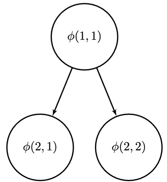
(a) Specification hierarchy graph

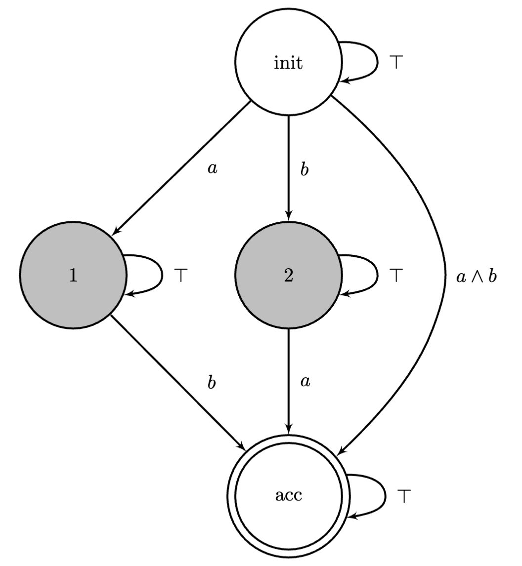
(b) NBA of LTL $\Diamond a\wedge\Diamond b$

Figure 1: Specification hierarchy graph and NBA. The specification hierarchy graph corresponds to hierarchical LTL specifications in Ex. 1. The NBA corresponds to the LTL specification in Ex. 3, where non-trivial decomposition states are colored in gray.

Definition IV.4 (Leaf and Non-leaf Specifications)

A specification is termed as a leaf specification if the associated node in the graph ${\mathcal{G}}_{h}$ does not have any children; otherwise, it is referred to as a non-leaf specification.

Lemma IV.5

Any hierarchical LTL specifications can be turned into a specification hierarchy graph.

Example 1

continued (Specification hierarchy graph)  The specification hierarchy graph is illustrated in Fig. 1(a). In this graph, $\phi({2},{1})$ and $\phi({2},{2})$ represent leaf specifications as well as composite propositions, while $\phi({1},{1})$ is categorized as a non-leaf specification. $\square$

The requirements on valid hierarchical LTL specifications are listed as follows:

Requirement 1 (Syntax)

The structure of hierarchical LTL specifications should satisfy:

1. The specification hierarchy graph is essentially a tree. That is, every specification, except for the topmost one, is exclusively contained within another specification as a composite proposition;

2. Leaf specifications comprise solely atomic propositions, while non-leaf specifications comprise solely composite propositions;

IV-B Semantics of Hierarchical LTL Specifications

We contend that hierarchical LTL formulas cannot be interpreted by simply substituting composite propositions with their corresponding specifications, as illustrated below.

Example 1

continued (Interpretation of Hierarchical LTL)  Continuing with Ex. 1, replacing composite propositions at level $1$ results in a flat specification $\phi({1},{1})=(\neg\Diamond a)\,\mathcal{U}\,(\Diamond b)$, which essentially equates to the specification $\Diamond b$. Therefore, such interpretation is not desirable. Another perspective to understanding hierarchical LTL is via its corresponding automatons. At level 2, the specification $\phi({2},{1})$ is considered satisfied when its corresponding automaton reaches an accepting state, which necessitates the atomic proposition $a$ becoming true. The same applies to $\phi({2},{2})$. At level 1, composite proposition $\phi({2},{1})$ must not be fulfilled before the satisfaction of $\phi({2},{2})$. In summary, this implies that atomic proposition $a$ should not be true before $b$. This perspective allows for the interpretation of each specification independently, where each composite proposition is treated as if it were an atomic proposition. $\square$

Example 2 (Two types of interpretation)

Consider the following specification at the top level:

$$\phi({1},{1})=\Diamond\phi({2},{1})\wedge\Diamond\phi({2},{2})\wedge\neg\phi({2},{1})\,\mathcal{U}\,\phi({2},{2}).$$

There are two distinct manners to interpret it. The first is a stricter interpretation where any transition in the automaton for the specification $\phi({2},{1})$ must not be enabled until the specification $\phi({2},{2})$ is fulfilled. The second interpretation is relaxed, allowing transitions in the automaton for $\phi({2},{1})$ to occur as long as $\phi({2},{2})$ is satisfied before the satisfaction of $\phi({2},{1})$. We opt for the latter, more flexible approach, as the former is a special case of the latter. $\square$

Requirement 2 (Semantics)

The semantics of hierarchical LTL specifications should satisfy that, for non-leaf specifications, it is sufficient that each composite proposition is satisfied at most once.

Requirement 2 prohibits expressions like $\phi_{1}\,\mathcal{U}\,\phi_{2}$ in non-leaf specifications that require multiple occurrences of satisfaction of composite proposition $\phi_{1}$. The intuition is that completing each robotic task once is sufficient in most cases. However, it is still permissible for leaf specifications to demand that atomic propositions be true multiple times, as in $\Diamond(a\wedge\bigcirc(a\,\mathcal{U}\,b))$.

Remark IV.6

Every co-safe LTL formula can be transformed into a Deterministic Finite Automaton (DFA). We opt for NBA, a form of Nondeterministic Finite Automaton (NFA), because co-safe LTLs are transformable into either DFAs or NFAs, making both equally expressive for expressing co-safe LTL formulas in this sense. Additionally, the work from Schillinger et al. [9] and the temporal order heuristic by Luo et al. [23] that our approach in Sec. VI is based on, utilize NFAs. Nonetheless, our approach can easily be adapted to work with DFAs as well, as graphically speaking, NFAs are more complex than DFAs.

Input: Hierarchical LTL specifications $\Phi$, state-specification plan $\tau$

Output: True or False

1 $\Phi^{acc}=\varnothing$ ;

2 for $i\in\{0,\ldots,h\}$  do

3       for $k\in\{K,\ldots,1\}$  do

4             $\Phi^{acc,k}=\varnothing$ ;

5             for $\phi\in\Phi^{k}\setminus\Phi^{acc}$  do

6                   if $k=K$  then

7                         $S(i)=\left\{s_{r}^{i}\,|\,(s_{r}^{i},\phi)\in\tau^{i}\right\}$ ;

8                         if $S(i)=\varnothing$ then

9                               continue;

10                              

11                         $\pi^{i}=\left\{L_{r}(s_{r}^{i})\,|\,s_{r}^{i}\in S(i)\right\}$ ;

12                        

13                  else

14                         $\pi^{i}=\Phi^{acc,k+1}$ ;

15                        

16                   ${\mathcal{Q}}_{\mathcal{B}}^{i+1}(\phi)=\left\{q^{\prime}\,|\,(q,\pi^{i},q^{\prime})\in\to_{\mathcal{B}}(\phi),\,\forall q\in{\mathcal{Q}}_{\mathcal{B}}^{i}(\phi),\right.$ $\left.\forall q^{\prime}\in{\mathcal{Q}}_{\mathcal{B}}(\phi)\right\}$ ;

17                   if ${\mathcal{Q}}^{i+1}_{\mathcal{B}}(\phi)\cap{\mathcal{Q}}_{\mathcal{B}}^{F}(\phi)\neq\varnothing$  then

18                         $\Phi^{acc,k}=\Phi^{acc,k}\cup\{\phi\}$ ;

19                        

20            $\Phi^{acc}=\Phi^{acc}\cup\Phi^{acc,k}\,\cup\,\texttt{Children}(\Phi^{acc,k})$ ;

21            

22      if $\phi({1},{1})\in\Phi^{acc}$ then

23             return True ;

24            

25return False ;

Algorithm 1 Satisfaction check

Given the presence of multiple specifications in hierarchical LTL, a robot could be addressing any particular specification at a specific state. To clarify the robot’s intention and facilitate the checking of satisfaction, we associate the state $s_{r}$ of a robot $r$ with a leaf specification $\phi_{r}\in\Phi^{K}$. This association forms a state-specification pair $(s_{r},\phi_{r})$, signifying that the robot $r$ is engaged in fulfilling the specification $\phi_{r}$ at state $s_{r}$.

Definition IV.7 (State-Specification Plan)

A state-specification plan with a horizon $h$, represented as $\tau$, is a timed sequence $\tau=\tau^{0}\tau^{1}\tau^{2}\ldots\tau^{h}$. Here, $\tau^{i}=((s_{1}^{i},\phi_{1}^{i}),(s_{2}^{i},\phi_{2}^{i}),\ldots,(s_{N}^{i},\phi_{N}^{i}))$ encapsulates the collective state-specification pairs of $N$ robots at the $i$-th timestep, where $s_{r}^{i}\in{\mathcal{S}}_{r}$, and $\phi_{r}^{i}\in\Phi^{K}\cup\{\epsilon\}$, with $\epsilon$ indicating the robot’s non-involvement in any leaf specification at that time.

Given a robot state-specification plan, the method for determining the satisfaction of hierarchical LTL specifications is shown in Alg. 1. Because the truth of a non-leaf specification depends solely on the specifications at the immediately lower level, the algorithm iteratively assesses specifications in a bottom-up manner. Alg. 1 will stop early and return true if the highest-level specification is met [lines 1-1]. This is because that all specifications belong to co-safe LTL, the subsequent plan becomes irrelevant once a specification is satisfied, eliminating the need for further satisfaction checks. Let $\Phi^{acc}$ represent the set of specifications that have been satisfied up to the current point [line 1]. Additionally, let $\Phi^{acc,k}$ denote the set of specifications at level $k$ that have just become satisfied at the current time step $i$ [line 1]. Iterating over each specification $\phi\in\Phi^{k}\setminus\Phi^{acc}$ at level $k$ that remain unsatisfied, Alg. 1 computes the reachable set of automaton states for the next time step, designated as ${\mathcal{Q}}^{i+1}_{\mathcal{B}}(\phi)$, to evaluate its satisfaction [lines 1-1]. This assessment varies depending on whether the specification $\phi$ is a leaf one or not. If the specification is a leaf specification, the algorithm aggregates the set of true propositions $\pi^{i}$, which are atomic propositions derived from the states of robots engaged in the specification $\phi$ [lines 1-1]. Otherwise, if the specification is not a leaf, the set of true propositions is identified as the set $\Phi^{acc,k+1}$ – these are the specifications at the immediate lower level that have just been satisfied [line 1]. The set $\Phi^{acc,k}$ gets updated if the reachable automaton states include at least one accepting state of $\phi$ [lines 1]. Following the completion of iterations over level $k$, the set $\Phi^{acc}$ is then updated [line 1], where $\texttt{Children}(\Phi^{acc,k})$ denotes the set of specifications that are children nodes in the specification hierarchy graph of any specification in $\Phi^{acc,k}$, that is, the set of specifications for which a path exists from any specification in $\Phi^{acc,k}$. The reason for including $\texttt{Children}(\Phi^{acc,k})$ is that, according to Requirement (2), it is sufficient for each specification to be satisfied just once. Consequently, there is no need to verify the satisfaction of a specification if its parent specification has already been satisfied. For instance, there is no need to verify the satisfaction of $\phi({2},{1})$ for the specification $\phi({2},{1})\vee\phi({2},{2})$ if $\phi({2},{2})$ becomes true.

Example 1

continued (Satisfaction Check) We observe that the specification $\phi({1},{1})$ is considered satisfied once $\phi({2},{2})$ becomes true, provided that $\phi({2},{1})$ remains false until that point. Consequently, verifying the satisfaction of $\phi({2},{1})$ becomes unnecessary (indeed, it should remain false) if its parent specification $\phi({1},{1})$ is already satisfied. $\square$

Theorem IV.8 (Expressivity Analysis)

Given the same set of atomic propositions ${\mathcal{A}}{\mathcal{P}}$ and based on the satisfaction check Alg. 1, the class of languages accepted by flat sc-LTL specifications is a subset of the class of languages accepted by hierarchical sc-LTL specifications.

Proof:

We first show that, for any flat sc-LTL, there exists an equivalent hierarchical counterpart. Therefore, the hierarchical sc-LTL is, at least, as expressive as its flat counterpart. Given a flat sc-LTL $\phi$, an equivalent two-level hierarchical sc-LTL can be constructed in a straightforward manner, where the top level is $\Diamond\phi$ and the bottom level is $\phi$ itself, that is,

$$L_{1}:\quad \phi({1},{1})=\Diamond\phi({2},{1})$$

$$L_{2}:\quad \phi({2},{1})=\phi.$$

Next, we introduce a counter-example to demonstrate the absence of the flat equivalent for certain hierarchical sc-LTL specifications. Considering a set of two atomic propositions $\{a,b\}$, the following hierarchical LTL specifications include two mutually exclusive leaf specifications:

$$L_{1}:\quad \phi({1},{1})=\Diamond\phi({2},{1})\wedge\,\Diamond\,\phi({2},{2})$$

$$L_{2}:\quad \phi({2},{1})=\Diamond a\wedge\neg b\,\mathcal{U}\,a$$

$$\phi({2},{2})=\Diamond b\wedge\neg a\,\mathcal{U}\,b.$$

While leaf specifications are mutually exclusive, the introduction of the state-specification plan enables the association of each state with a specific specification. Hence, the satisfaction check Alg. 1 facilitates the separate treatment of these two leaf specifications. For example, when these two specifications are assigned to separate robots, they can be realistically fulfilled. However, when solely utilizing atomic propositions $a$ and $b$, combining two leaf specifications into a single, flat sc-LTL specification is unfeasible, as it inevitably results in a contradiction, reducing the specification to False. ∎

Remark IV.9

The method demonstrated in the proof for transforming a flat specification into a hierarchical one is straightforward but of limited use. Exploring the conversion process between flat and hierarchical formats is worthwhile, although it falls outside the current scope.

Remark IV.10

The requirements on syntax and semantics for hierarchical LTL specifications in this work are specifically designed for the field of robotics and may not be directly applicable to other domains. Exploring the construction of hierarchical LTL from task specifications is an interesting topic for future research. Our experience indicates that a top-down reasoning approach, similar to Hierarchical Task Network (HTN) analysis, is effective. This method entails recognizing the inclusion relationships among tasks and organizing them into various levels of abstraction, ranging from general to specific. At each level, tasks that are closely related should be combined into single flat formulas, while those with weaker connections should be grouped into separate flat formulas.

V Problem Formulation

To formulate the problem, we first introduce a variant of the product team model defined in work [9], which aggregates the set of PBA for a given specification. Following this, we expand upon this concept to develop the hierarchical team model, which integrates a set of product team models to address hierarchical LTL specifications.

V-A Product Team Model

Inspired by work [9], we make the following assumption on every leaf specifications.

Assumption V.1 (Decomposition)

Every leaf specification $\phi\in\Phi^{K}$ can be decomposed into a set of tasks such that

• Independence: every task can be executed independently;

• Completeness: completion of all tasks, irrespective of the order, satisfies the leaf specification $\phi$.

Definition V.2 (Decomposition Set [9])

The decomposition set ${\mathcal{D}}_{\mathcal{B}}\subseteq{\mathcal{Q}}_{\mathcal{B}}$ of the NBA ${\mathcal{B}}$ contains all states $q$ such that each state leads to a decomposition of tasks.

Example 3 (Decomposition Set)

Consider an LTL specification $\phi=\Diamond a\wedge\Diamond b$, with its corresponding NBA depicted in Fig. 1(b). For any two-part satisfying word $\sigma=\sigma_{1}\sigma_{2}$, where $\sigma_{1}$ leads to a run ending at state 2, the reverse sequence $\sigma_{2}\sigma_{1}$ also satisfies the specification by leading to a run through state 1. This indicates that the tasks before and after state 2 can be completed in any order. Therefore, state 2 belongs to the decomposition set. Similarly, state 1 also belongs to the decomposition set. By default, all initial and accepting states in an NBA are considered decomposition states. $\square$

Definition V.3 (Product Team Model (modified from [9]))

Given a leaf specification $\phi\in\Phi^{K}$, the product team model ${\mathcal{P}}(\phi)$ consists of $N$ product models ${\mathcal{P}}(r,\phi)$ and is given by the tuple ${\mathcal{P}}(\phi):=({\mathcal{Q}}_{{\mathcal{P}}},{\mathcal{Q}}^{0}_{\mathcal{P}},\to_{{\mathcal{P}}},{\mathcal{Q}}^{F}_{{\mathcal{P}}})$:

• ${\mathcal{Q}}_{{\mathcal{P}}}=\left\{(r,s,q):r\in[N],(s,q)\in{\mathcal{Q}}_{\mathcal{P}}(r,\phi)\right\}$ is the set of state;

• ${\mathcal{Q}}^{0}_{\mathcal{P}}=\left\{(r,s,q)\in{\mathcal{Q}}_{\mathcal{P}}:r=1,(s,q)\in{\mathcal{Q}}_{\mathcal{P}}^{0}(1,\phi)\right\}$ is the set of initial states ;

• $\to_{\mathcal{P}}\,\in{\mathcal{Q}}_{{\mathcal{P}}}\times{\mathcal{Q}}_{{\mathcal{P}}}$ is the transition relation. One type of transition, referred to as in-spec transitions, occurs inside a PBA. That is, $(r,s,q)\to_{\mathcal{P}}(r,s^{\prime},q^{\prime})$ if $(s,q)\to_{{\mathcal{P}}(r,\phi)}(s^{\prime},q^{\prime})$; the other type of transition relation, denoted by $\zeta_{\text{in}}$, occurs between two PBAs and is defined below in Def. V.4;

• ${\mathcal{Q}}^{F}_{{\mathcal{P}}}=\{(r,s,q)\in{\mathcal{Q}}_{\mathcal{P}}:q\in{\mathcal{Q}}^{F}_{\mathcal{B}}(\phi)\}$ is the set of accepting/final states ;

Definition V.4 (In-Spec Switch Transition (modified from [9]))

Given a specification $\phi$, the set of in-spec switch transitions in ${\mathcal{P}}(\phi)$ is given by $\zeta_{\text{in}}\subset{\mathcal{Q}}_{\mathcal{P}}\times{\mathcal{Q}}_{\mathcal{P}}$. A transition $\left((r,s,q),(r^{\prime},s^{\prime},q^{\prime})\right)$ belongs to $\zeta_{\text{in}}$ if and only if it:

• points to the next robot, $r^{\prime}=r+1$;

• preserves the NBA progress, $q=q^{\prime}$;

• represents a decomposition choice, $q\in{\mathcal{D}}_{\mathcal{B}}(\phi)$.

The distinction between in-spec transitions and in-spec switch transitions lies in their impact on task progress: in-spec transitions advance the task through the same robot, while in-spec switch transitions involve changing to a different robot without altering the task’s progress, as indicated by $q=q^{\prime}$. A visual representation of ${\mathcal{P}}(r,\phi)$ can be found in Fig. 2. The connections between product models are unidirectional, starting from the first robot and ending at the last robot. The specific arrangement of robots is irrelevant. Transitioning to the next product model occurs solely at in-spec switch transitions. Any path connecting an initial to an accepting state constitutes a feasible solution, comprising multiple path segments. Both the start and end state of each path segment have automaton states that belong to the decomposition set. Each segment results in a sequence of actions for an individual robot. These action sequences can be executed in parallel as they collectively decompose the overall task, as illustrated in Fig. 2.

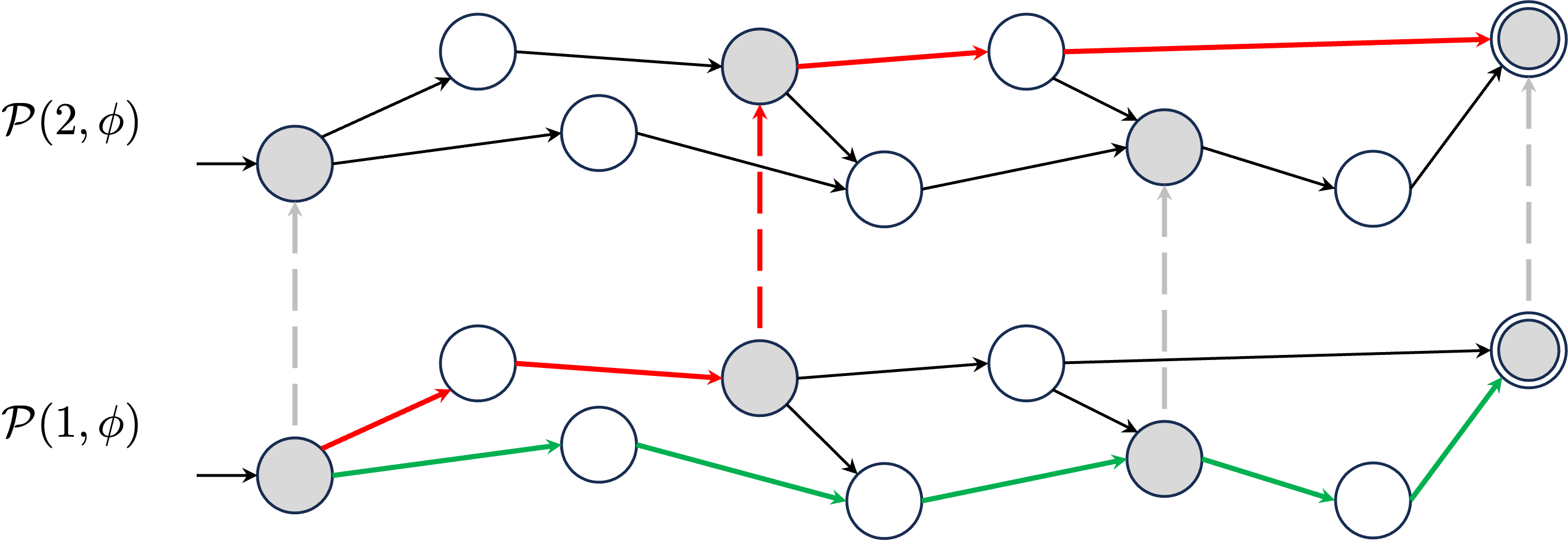
Figure 2: The product team model featuring two robots. PBAs ${\mathcal{P}}(1,\phi)$ and ${\mathcal{P}}(2,\phi)$ may be different reflecting the robots’ heterogeneity. Initial states are indicated with incoming arrows, and accepting states are depicted with double circles. The decomposition sets are highlighted in gray. In-spec switch transitions are represented by dashed arrows. A plan exclusive to robot 1 is traced by the green path, whereas the red path delineates a plan that involves the collaboration of both robots.

Remark V.5

Note that we construct team models exclusively for leaf specifications which directly involve atomic propositions. The switch transitions described in [9] point to the initial state of the next robot, that is, $s^{\prime}=s_{r^{\prime}}^{0}$, which is not the case for the in-spec switch transitions in our work. This difference arises because Schillinger et al. [9] address scenarios with a single specification, where a robot typically starts a task from its initial state. In contrast, in scenarios involving multiple specifications, a robot can begin a new task from its last state at the end of the preceding task.

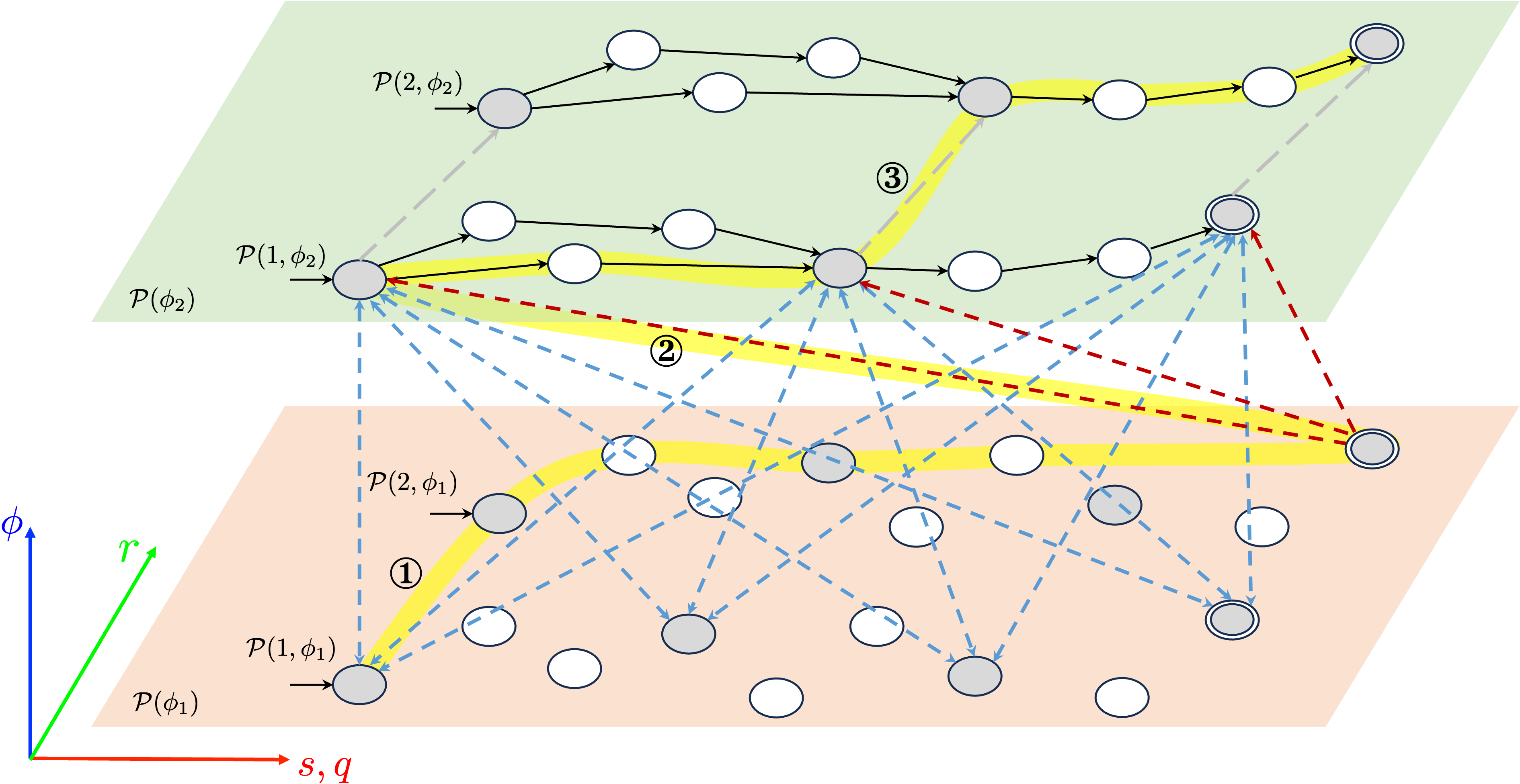
Figure 3: Hierarchical team models for two leaf specifications and two robots. The product team models for each leaf specification are depicted within areas shaded in light orange and green. To enhance clarity, some transitions within a single PBA are omitted. Inter-spec type I and II switch transitions are illustrated using blue and red dashed arrows, respectively. It’s important to note that type I switch transitions are bidirectional, while type II switch transitions are unidirectional. For the sake of readability, inter-spec type I switch transitions are specifically shown for ${\mathcal{P}}(1,\phi_{1})$ and ${\mathcal{P}}(1,\phi_{2})$. Inter-spec type II switch transitions are only shown from ${\mathcal{P}}(2,\phi_{1})$ to ${\mathcal{P}}(1,\phi_{2})$. The path marked in yellow highlights a specific plan. This plan originates from the initial state of ${\mathcal{P}}(1,\phi_{1})$ and concludes at the accepting state of ${\mathcal{P}}(2,\phi_{2})$. This path involves assigning robot 2 to fulfill the specification $\phi_{1}$, which includes one in-spec switch transition ①. Subsequently, robots 1 and 2 are tasked with satisfying specification $\phi_{2}$, connected through a type II inter-spec switch transition ② and involving another in-spec switch transition ③.

V-B Hierarchical Team Models

To extend to hierarchical LTL specifications, we construct a product team model for each leaf specification. The goal in this section is to connect them to form a connectable space. We refer to the scenario of decomposition of tasks for one specifications as in-spec independence. In contrast, leaf specifications can exhibit dependencies. For example, one leaf specification $\phi$ might need to be completed before another $\phi^{\prime}$. This scenario is referred to as inter-spec dependence. This distinguishes us from that of [9], where tasks are executed without coordination among robots, limiting their ability to address complex collaborative tasks. Another scenario is inter-spec independence, where two leaf specifications are unrelated and can be satisfied independently. We note that in-spec dependence does not exist, as precluded by Asm. V.1. To capture inter-spec dependency and independence, we introduce two additional types of switch transitions between different product team models.

Definition V.6 (Hierarchical Team Models)

Given the hierarchical LTL specifications $\Phi$, the hierarchical team models ${\mathcal{P}}$ consists of a set of product team models ${\mathcal{P}}(\phi)$ with $\phi\in\Phi^{K}$ and is denoted by the tuple ${\mathcal{P}}:=({\mathcal{Q}}_{{\mathcal{P}}},{\mathcal{Q}}^{0}_{\mathcal{P}},\to_{{\mathcal{P}}},{\mathcal{Q}}^{F}_{{\mathcal{P}}})$:

• ${\mathcal{Q}}_{{\mathcal{P}}}=\left\{(r,\phi,s,q):\phi\in\Phi^{K},(r,s,q)\in{\mathcal{Q}}_{\mathcal{P}}(\phi)\right\}$ is the set of state;

• ${\mathcal{Q}}^{0}_{\mathcal{P}}=\left\{(r,\phi,s,q)\in{\mathcal{Q}}_{\mathcal{P}}:\phi\in\Phi^{K},(r,s,q)\in{\mathcal{Q}}_{\mathcal{P}}^{0}(\phi)\right\}$ is the set of initial states ;

• $\to_{\mathcal{P}}\,\in{\mathcal{Q}}_{{\mathcal{P}}}\times{\mathcal{Q}}_{{\mathcal{P}}}$ is the transition relation. One type of transition occurs inside a product team model, that is, $(r,\phi,s,q)\to_{\mathcal{P}}(r^{\prime},\phi,s^{\prime},q^{\prime})$ if $(r,s,q)\to_{{\mathcal{P}}(\phi)}(r^{\prime},s^{\prime},q^{\prime})$; another two types of transition relation, denoted by $\zeta_{\text{inter}}^{1}$ and $\zeta_{\text{inter}}^{2}$, occur between two product teams models and are defined below in Def. V.7 and V.8;

• ${\mathcal{Q}}^{F}_{{\mathcal{P}}}=\{(r,\phi,s,q)\in{\mathcal{Q}}_{\mathcal{P}}:q\in{\mathcal{Q}}^{F}_{\mathcal{B}}(\phi)\}$ is the set of accepting/final states.

Definition V.7 (Inter-Spec Type I Switch Transition)

A transition, denoted by $\zeta_{\text{inter}}^{1}=\left((r,\phi,s,q),(r^{\prime},\phi^{\prime},s^{\prime},q^{\prime})\right)$, is type I switch transition if and only if it:

• connects the same robots, $r=r^{\prime}$;

• points to two different leaf specifications, $\phi\neq\phi^{\prime}$;

• points to the same robot state, $s=s^{\prime}$;

• connects two decomposition states, $q\in{\mathcal{D}}_{\mathcal{B}}(\phi),q^{\prime}\in{\mathcal{D}}_{\mathcal{B}}(\phi^{\prime})$.

Definition V.8 (Inter-Spec Type II Switch Transition)

A transition, denoted by $\zeta_{\text{inter}}^{2}=\left((r,\phi,s,q),(r^{\prime},\phi^{\prime},s^{\prime},q^{\prime})\right)$, is type II switch transition if and only if it:

• points to the first robot, $r^{\prime}=1$;

• points to two different leaf specifications, $\phi\neq\phi^{\prime}$;

• connects an accepting state to a decomposition state, $q\in{\mathcal{Q}}_{\mathcal{B}}^{F}(\phi),q^{\prime}\in{\mathcal{D}}_{\mathcal{B}}(\phi^{\prime})$.

Inter-spec type I switch transitions enable switching to another PBA with a different leaf specification, while retaining the same robot and pausing the current task. Conversely, inter-spec type II switch transitions create a connection from the accepting state of one PBA to the decomposition state of another PBA associated with the first robot, indicating the completion of one specification and the resumption of another. These hierarchical team models can be graphically represented in a 3D space, with each product team model occupying a 2D plane; see Fig. 3. This structure encompasses three axes: one representing the progress of a task for a specific specification (the $(s,q)$-axis), another indicating the assignment of tasks among different robots (the $r$-axis), and the last one tracking the overall progress of tasks across different specifications (the $\phi$-axis).

Remark V.9

The construction is not merely a product of all NBA states and robot states. Instead, if each product team model is considered a distinct sub-space, the inter-spec switch transitions facilitate the connections between these sub-spaces. As a result, two consecutive product models are only loosely interconnected. The majority of states across different sub-spaces remain disconnected. Such a design significantly reduces the overall search space, enhancing the efficiency of the subsequent search.

Given a state-specification plan $\tau=\tau^{0}\tau^{1}\ldots\tau^{h}$ where $\tau^{i}=((s_{1}^{i},\phi_{1}^{i}),(s_{2}^{i},\phi_{2}^{i}),\ldots,(s_{N}^{i},\phi_{N}^{i}))$, the additive cost, such as energy consumption, is defined as

$$J(\tau)=\sum_{i=0}^{h-1}c(\tau^{i},\tau^{i+1})=\sum_{i=0}^{h-1}\sum_{r=1}^{N}c_{r}(s^{i}_{r},s^{i+1}_{r}),$$ (3)

where $c_{r}(s^{i}_{r},s^{i+1}_{r})$ is the cost between states for robot $r$. Finally, the problem in this work we aim to solve can be formulated as follow:

Problem 1

Given the hierarchical team models ${\mathcal{P}}$, derived from transition systems of robots and the NBAs of hierarchical LTL specifications $\Phi$, find an optimal state-specification plan $\tau^{*}$ that minimizes $J(\tau^{*})$ and satisfies $\Phi$.

VI Search-based STAP under Hierarchical LTL Specifications

This section begins by introducing a search-based approach, which constructs hierarchical team models on the fly, ensuring both completeness and optimality; see Sec. VII. Subsequently, we discuss several heuristics designed to expedite the search process.

VI-A On-the-fly Search

Input: Hierarchical LTL specifications $\Phi$, a set of robots $[N]$

Output: state-specification plan

1 ${\mathcal{V}}_{\text{seen}}=\varnothing,{\mathcal{V}}_{\text{explored}}=\varnothing,{\mathcal{H}}_{\text{front}}=\varnothing,\Lambda_{\text{explored}}=\varnothing$ ;

2 ${\mathcal{V}}_{\text{init}}=\{v\,|\,(r,\phi,{\mathbf{s}}(r),{\mathbf{q}}(\phi))\in{\mathcal{Q}}_{\mathcal{P}}^{0},\forall r\in[N],\forall\phi\in\Phi^{K}\wedge{\mathbf{q}}(\phi)\in{\mathcal{Q}}_{\mathcal{B}}^{0}(\phi),\forall\phi\in\Phi\setminus\Phi^{K}\}$ ;

3 ${\mathcal{H}}_{\text{front}}.\texttt{push}(({\mathcal{V}}_{\text{init}},0))$;

4 $\tau_{\text{explored}}(v)=v,\forall v\in{\mathcal{V}}_{\text{init}}$;

5 Build hierarchy specification graph ${\mathcal{G}}_{h}$;

6 while ${\mathcal{H}}_{\text{front}}\neq\varnothing$ do

7       $(v,c_{v})={\mathcal{H}}_{\text{front}}.{\texttt{pop}}()$;

8       if $v\in{\mathcal{V}}_{\text{explored}}$ then

9             continue;

10            

11      ${\mathcal{V}}_{\text{explored}}.\texttt{add}(v)$;

12       if $v.{\mathbf{q}}(1,1)\in{\mathcal{Q}}_{\mathcal{B}}^{F}(1,1)$ then

13             return $\texttt{ExtractPlan}(\Lambda_{\text{explored}}(v))$ ;

14            

15      ${\mathcal{V}}_{\text{succ}}=\texttt{GetSucc}(v,{\mathcal{P}},{\mathcal{G}}_{h})$ ;

16       for $(u,c_{vu})\in{\mathcal{V}}_{\text{succ}}$  do

17             $c_{u}=c_{v}+c_{vu}$;

18             if $u\not\in{\mathcal{V}}_{\text{seen}}$ or $c_{u}<{\mathcal{V}}_{\text{seen}}(u)$  then

19                   ${\mathcal{V}}_{\text{seen}}(u)=c_{u}$;

20                   ${\mathcal{H}}_{\text{front}}.\texttt{push}((u,c_{u}))$;

21                   $\Lambda_{\text{explored}}(u)=\Lambda_{\text{explored}}(v)+u$ ;

22                  

23return $\varnothing$;

Algorithm 2 Search-based STAP

The on-the-fly search algorithm we propose is built upon the Dijkstra’s algorithm, as detailed in Alg. 2. The search state is defined as $v=(r,\phi,{\mathbf{s}},{\mathbf{q}})$, where ${\mathbf{s}}\in{\mathcal{S}}_{1}\otimes\ldots\otimes{\mathcal{S}}_{N}$ and ${\mathbf{q}}={\mathcal{Q}}_{\mathcal{B}}(\phi({K},{1}))\otimes\ldots\otimes{\mathcal{Q}}_{\mathcal{B}}(\phi({1},{1}))$. This state is comprised of three parts: the first part, $(r,\phi)$, indicates the specific PBA currently being searched; the second part, ${\mathbf{s}}$, represents the states of all robots; and the third part, ${\mathbf{q}}$, denotes the automaton states of all specifications (including leaf and non-leaf ones). Two states are considered equivalent if they share the same $r$, $\phi$, ${\mathbf{s}}$, and ${\mathbf{q}}$ values. The notation ${\mathbf{s}}(r)$ and ${\mathbf{q}}(\phi({k},{i}))$ refer to the state of robot $r$ and the automaton state of specification $\phi({k},{i})$ reached so far, respectively. We use ${\mathcal{V}}_{\text{explored}}$ and ${\mathcal{V}}_{\text{seen}}$ to denote the sets of states that have been explored and seen, and ${\mathcal{H}}_{\text{front}}$ for the states awaiting exploration. States within ${\mathcal{H}}_{\text{front}}$ are ordered by their associated costs. Lastly, $\Lambda_{\text{explored}}$ maps each explored state to the shortest path that led to it.

Input: state $v$, hierarchical team models ${\mathcal{P}}$, hierarchy specification graph ${\mathcal{G}}_{h}$

Output: Set of successor states ${\mathcal{V}}_{\text{succ}}$

1 ${\mathcal{V}}_{\text{succ}}=\varnothing$;

2 $(r,\phi,s,q)=(v.r,v.\phi,v.{\mathbf{s}}(v.r),v.{\mathbf{q}}(v.\phi))$ ;

3

4$\Phi_{\text{prt}}=\texttt{Parents}({\mathcal{G}}_{h},\phi)$ ;

5 if $q\not\in{\mathcal{Q}}^{F}_{\mathcal{B}}(\phi)$ and $v.{\mathbf{q}}(\phi_{\text{prt}})\not\in{\mathcal{Q}}_{\mathcal{B}}^{F}(\phi_{\text{prt}}),\forall\phi_{\text{prt}}\in\Phi_{\text{prt}}$ then

       ;

        $\triangleright$ In-spec transitions in ${\mathcal{P}}(r,\phi)$

6       for $((s,q),(s^{\prime},q^{\prime}))\in\to_{{\mathcal{P}}(r,\phi)}$ do

7             $u=v,{\mathcal{V}}_{u}=\varnothing$;

8             $u.{\mathbf{s}}(r)=s^{\prime},\;u.{\mathbf{q}}(\phi)=q^{\prime}$ ;

9             $\pi=\{\phi\}$ if $q^{\prime}\in{\mathcal{Q}}^{F}_{\mathcal{B}}(\phi)$ else $\varnothing$ ;

10             $\texttt{UpdateNonLeafSpecs}(\pi,u,\Phi_{\text{prt}},{\mathcal{V}}_{u})$ ;

11             ${\mathcal{V}}_{\text{succ}}.\texttt{add}(({\mathcal{V}}_{u},c_{r}(s,s^{\prime})))$;

12            

      ;

        $\triangleright$ In-spec switch transitions in ${\mathcal{P}}(\phi)$

13       if $r\neq N$ and $((r,\phi,s,q),(r+1,\phi,v.{\mathbf{s}}(r+1),q))\in\zeta_{\text{in}}$ then

14             $u=v$;

15             $u.r=r+1$ ;

16             ${\mathcal{V}}_{\text{succ}}.\texttt{add}((u,0))$;

17            

;

  $\triangleright$ Type I switch transitions in ${\mathcal{P}}$

18 for $\phi^{\prime}\in\Phi^{K}\setminus\{\phi\}$  do

19       if $((r,\phi,s,q),(r,\phi^{\prime},s,v.{\mathbf{q}}(\phi^{\prime}))\in\zeta_{\text{inter}}^{1}$ then

20             $u=v$;

21             $u.\phi=\phi^{\prime}$ ;

22             ${\mathcal{V}}_{\text{succ}}.\texttt{add}((u,0))$;

23            

;

  $\triangleright$ Type II switch transitions in ${\mathcal{P}}$

24 for $\phi^{\prime}\in\Phi^{K}\setminus\{\phi\}$  do

25       if $((r,\phi,s,q),(1,\phi^{\prime},v.{\mathbf{s}}(1),v.{\mathbf{q}}(\phi^{\prime}))\in\zeta_{\text{inter}}^{2}$ then

26             $u=v$;

27             $u.r=1,\;u.\phi=\phi^{\prime}$ ;

28             ${\mathcal{V}}_{\text{succ}}.\texttt{add}((u,0))$;

29            

30return ${\mathcal{V}}_{\text{succ}}$;

Algorithm 3 $\texttt{GetSucc}(v,{\mathcal{P}},{\mathcal{G}}_{h})$

Definition VI.1 (Initial State)

A state $v=(r,\phi,{\mathbf{s}},{\mathbf{q}})$ is an initial state if

• $(r,\phi,{\mathbf{s}}(r),{\mathbf{q}}(\phi))\in{\mathcal{Q}}_{\mathcal{P}}^{0},\forall r\in[N],\forall\phi\in\Phi^{K}$;

• ${\mathbf{q}}(\phi)\in{\mathcal{Q}}_{\mathcal{B}}^{0}(\phi),\forall\phi\in\Phi\setminus\Phi^{K}$.

That is, all robots begin at their initial states, and every specification starts from its initial automaton state [line 2]. Whenever a state $v$ is popped out from the set ${\mathcal{H}}_{\text{front}}$ for exploration, it is added to the set of explored states if it hasn’t been already [lines 2-2]. The iteration process concludes when an accepting state of the topmost-level specification is reached. At this point, the function ExtractPlan is employed to parallelize the sequentially searched path, generating a state-specification plan [line 2]. If the accepting state is not yet reached, the algorithm proceeds to determine the successor states of $v$, along with their associated transition costs [line 2], through the function GetSucc, outlined in Alg. 3. For each successor state that is either unseen or has a total cost lower than previously found, it is queued into ${\mathcal{H}}_{\text{front}}$ for future exploration. Concurrently, the corresponding path leading to this state is recorded [lines 2-2].

The function GetSucc determines the successor states of a given state $v=(r,\phi,{\mathbf{s}},{\mathbf{q}})$ by considering in-spec transitions in ${\mathcal{P}}(r,\phi)$, in-spec switch transitions in ${\mathcal{P}}(v.\phi)$, and inter-spec type I and II switch transitions in ${\mathcal{P}}$. To identify in-spec transitions in ${\mathcal{P}}(r,\phi)$, the function initially checks if the specification $\phi$ or any of its non-leaf parent specifications are satisfied. This is achieved using Parents(${\mathcal{G}}_{h}$, $\phi$), which returns the path from the leaf specification $\phi$ to the topmost specification in the hierarchical specification graph ${\mathcal{G}}_{h}$, excluding $\phi$ itself [line 3]. If $\phi$ or any of its parent specifications are satisfied, the search in ${\mathcal{P}}(r,\phi)$ and ${\mathcal{P}}(\phi)$ ceases, as further exploration is unnecessary. This is based on requirements (1) and (2), which state that each leaf specification appears only once in a non-leaf specification and satisfying each specification once is sufficient. If a parent specification is satisfied, the leaf specification no longer contributes to task progression.

Input: True composite propositions $\pi$, state $u$, parent specifications $\Phi_{\text{prt}}$

Output: Updated set of states ${\mathcal{V}}_{u}$

1 $\phi_{\text{prt}}=\Phi_{\text{prt}}.\texttt{pop}()$ ;

2 ${\mathcal{Q}}_{\mathcal{B}}^{\text{succ}}=\left\{q^{\prime}\,|\,(u.{\mathbf{q}}(\phi_{\text{prt}}),\pi,q^{\prime})\in\to_{\mathcal{B}}(\phi_{\text{prt}}),\forall q^{\prime}\in{\mathcal{Q}}_{\mathcal{B}}(\phi_{\text{prt}})\right\}$;

3 for $q^{\prime}\in{\mathcal{Q}}^{\text{succ}}_{\mathcal{B}}$ do

4       $u.{\mathbf{q}}(\phi_{\text{prt}})=q^{\prime}$ ;

5       if $\phi_{\text{prt}}=\phi(1,1)$ then

6             ${\mathcal{V}}_{u}.\texttt{add}(u)$ ;

7            

8      else

9             $\pi=\{\phi_{\text{prt}}\}$ if $q^{\prime}\in{\mathcal{Q}}^{F}_{\mathcal{B}}(\phi_{\text{prt}})$ else $\varnothing$;

10             $\texttt{UpdateNonLeafSpecs}(\pi,u,\Phi_{\text{prt}},{\mathcal{V}}_{u})$;

11            

Algorithm 4 $\texttt{UpdateNonLeafSpecs}(\pi,u,\Phi_{\text{prt}},{\mathcal{V}}_{u}$)

If none of the parent specifications are satisfied, the state of robot $r$ in $v.{\mathbf{s}}$ and the automaton state of leaf specification $\phi$ in $v.{\mathbf{q}}$ are updated based on in-spec transitions in $\to_{{\mathcal{P}}(r,\phi)}$ [line 3]. Subsequently, the automaton states of all parent specifications of $\phi$ are also updated, as detailed in lines 3-3 and further elaborated in Alg. 4. For the three types of switch transitions, only the robot $r$ (in the case of in-spec switch transitions [line 3)], the leaf specification $\phi$ (for inter-spec type I switch transitions [line 3]), or both robot $r$ and specification $\phi$ (for inter-spec type II switch transitions [line 3]) are updated. This implies a shift in the search space to a different PBA, without modifying $v.{\mathbf{s}}$ and $v.{\mathbf{q}}$. Since these transitions do not change robot states and automaton states, the function UpdateNonLeafSpecs is not invoked.

Given a state $u$ and the set of parent specifications $\Phi_{\text{prt}}$ of the leaf specification $u.\phi$ currently being explored, the function UpdateNonLeafSpecs utilizes a depth-first strategy to refresh the automaton states of non-leaf specifications within $\Phi_{\text{prt}}$. When considering a specific parent specification $\phi_{\text{prt}}\in\Phi_{\text{prt}}$, the function initially identifies all states that can be reached based on the acceptance of the preceding specification at the immediate lower level [lines 4-4]. The automaton state of $\phi_{\text{prt}}$ in $u.{\mathbf{q}}$ is then updated using these reachable states [line 4]. This process continues until the automaton state of the topmost specification is updated [line 4].

Input: Searched path $\Lambda$

Output: state-specification plan $\tau$

1 Remove switch states from $\Lambda$ and divide $\Lambda$ into $l$ path segments with each sharing the same specification ;

2 for $k\in[l]$ do

3       for $v\in\Lambda_{k}$ do

4             $\tau^{i}=((s_{1}^{i},\phi_{1}^{i}),\ldots,(s_{r}^{i},\phi_{r}^{i}),\ldots,(s_{N}^{i},\phi_{N}^{i}))$ where $(s_{r}^{i},\phi_{r}^{i})=(v.{\mathbf{s}}(r),v.\phi)$ and $(s_{r^{\prime}}^{i},\phi_{r^{\prime}}^{i})=(v.{\mathbf{s}}(r^{\prime}),\epsilon),\forall r^{\prime}\not=v.r$ ;

5            

6return $\tau$;

Algorithm 5 $\texttt{ExtractPlan}(\Lambda)$

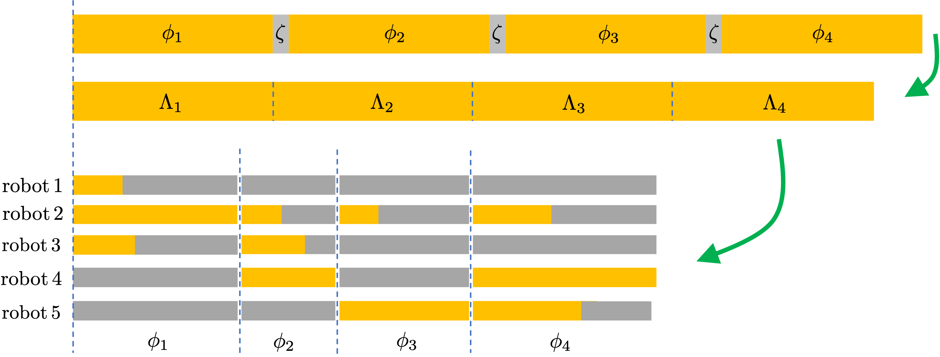
Figure 4: The process of plan extraction is depicted as follows: The top bar represents the path, segmented by inter-spec switch transitions, with each segment corresponding to distinct specifications. The middle bar illustrates the path after removing switch states. At the bottom, the derived plan for a team of five robots is displayed. Here, orange segments indicate active periods for the robots, while gray segments represent their inactive phases.

The ExtractPlan function in Alg. 5 processes the path $\Lambda=v_{0}v_{1}\ldots v_{n}$, which leads to the state satisfying the topmost specification, and outputs a state-specification plan $\tau$. This process is visually represented in Fig. 4. A state $v$ within $\Lambda$ is identified as a switch state if it is the end state of an inter-spec switch transition $\zeta_{\text{inter}}^{1}\cup\zeta_{\text{inter}}^{2}$, which has the same robot state and automaton state as the corresponding start state. The path $\Lambda$ is segmented by these switch states, with each segment corresponding to states associated with the same specification, indicative of a search within a specific product team model. To create a concise path $\Lambda^{\prime}$, all switch states are removed, as they merely facilitate transitions between product team models and don’t influence the plan’s progress. This refined path is denoted as $\Lambda^{\prime}=\Lambda_{1}\Lambda_{2}\ldots\Lambda_{l}$, where $\Lambda_{k}$ represents the $k$-th path segment, as shown in line 5. The next step involves converting these sequential path segments into parallel executions. For each segment $\Lambda_{k}$, we identify all active robots ${\mathcal{R}}_{k}$ participating in the specification $\phi_{k}$, represented as ${\mathcal{R}}_{k}=\left\{v.r\,|\,v\in\Lambda_{k}\right\}$. Due to task decomposition [9], each robot in ${\mathcal{R}}_{k}$ can execute its part of the plan independently. Robots not in ${\mathcal{R}}_{k}$ are considered inactive for that segment. The overall plan horizon post-parallelization is determined by the longest path among all active robots. Note that an active robot might not maintain the active mode during the entire horizon if it completes its actions in a shorter time frame. For each robot state, we pair it with the relevant specification $\phi_{k}$ if the robot is active, or with a null specification $\epsilon$ if it’s inactive [line 5].

VI-B Search Acceleration with Heuristics

While our hierarchical team models utilize switch transitions to loosely connect different components, thereby enhancing efficiency, this section introduces three heuristics aimed at expediting the search.

VI-B1 Temporal Order between Specifications

Consider the topmost specification $\phi({1},{1})=\Diamond(\phi({2},{1})\wedge\Diamond\phi({2},{2}))$, where specification $\phi({2},{2})$ is required to be satisfied following the completion of $\phi({2},{1})$. Given this sequential requirement, a switch transition from the team model of specification $\phi({2},{2})$ to that of $\phi({2},{1})$ is unnecessary.

Given two leaf specifications $\phi_{1},\phi_{2}\in\Phi^{K}$, let $\phi_{1}\bowtie\phi_{2}$, where $\bowtie\,\in\{\prec,\succ,\|\}$, denote the case where specification $\phi_{1}$ should be completed prior to ($\prec$), after ($\succ$) or independently ($\|$) of $\phi_{2}$. To determine these temporal relationships between leaf specifications, we adopt the method in [33]. Following this, we remove all switch transitions from the product team model pertaining to specification $\phi_{1}$ to that of $\phi_{2}$ for cases where $\phi_{1}$ should not be satisfied prior to $\phi_{2}$, i.e., $\phi_{1}\succ\phi_{2}$. The effect of this pruning is that any task related to $\phi_{2}$ will be completed before initiating any task related to $\phi_{1}$.

VI-B2 Essential Switch Transitions

We introduce the concept of essential switch transitions to further refine the connections between PBAs.

Definition VI.2 (Essential State)

An essential state for robot $r$, denoted as $(r,s)$, is defined either (a) $s=s_{r}^{0}$ or (b) there exists a leaf specification $\phi$ fulfilling the conditions:

• $((\phi,r,s,q),(\phi,r,s,q^{\prime}))\in\to_{{\mathcal{P}}(r,\phi)}$;

• $q\neq q^{\prime}$;

• $q^{\prime}\in{\mathcal{D}}_{\mathcal{B}}(\phi)$.

This definition implies that an essential state is either (a) the initial state of robot $r$ or (b) a state where robot $r$ causes an in-spec transition to a decomposition state of a leaf specification for the first time. In the latter case, the intuition is that essential states are pivotal for achieving substantial progress in the task.

Definition VI.3 (Essential Switch Transition)

A switch transition $\zeta=\left((\phi,r,s,q),(\phi^{\prime},r^{\prime},s^{\prime},q^{\prime})\right)\in\zeta_{\text{in}}\cup\zeta_{\text{inter}}^{1}\cup\zeta_{\text{inter}}^{2}$ is an essential switch transition if both $(r,s)$ and $(r^{\prime},s^{\prime})$ are essential states.

Note that the leaf specifications $\phi$ and $\phi^{\prime}$ might not be the exact ones that render the states $(r,s)$ and $(r^{\prime},s^{\prime})$ essential. In other words, $\phi$ and $\phi^{\prime}$ could represent any leaf specifications, which is further explained in Ex. 4 below. Consequently, any switch transitions that are not deemed essential will be excluded from consideration.

Example 4

Consider a sequence of three transitions: $(\phi,r,s,q)\overset{\text{\char 172}}{\to}(\phi,r,s,q^{\prime})\overset{\text{\char 173}}{\to}(\phi^{\prime},r,s,q^{\prime\prime})\overset{\text{\char 174}}{\to}(\phi^{\prime},r+1,s^{\prime},q^{\prime\prime})$. Here, transition ① is an in-spec transition, transition ② is an inter-spec type I switch transition, and transition ③ is an in-spec switch transition. Let’s assume transition ① renders $(r,s)$ an essential state. If we strictly limit $(r,s)$ to be associated only with specification $\phi$, then transition ③ would not be classified as essential. Consequently, it would be excluded, potentially impacting the feasibility of the overall plan. $\square$

VI-B3 Guidance by Automaton States

Unlike the first two heuristics, which focus on reducing the graph size, the last heuristic aims to speed up the search process by prioritizing the expansion of more promising states — those that are closer to achieving satisfaction. For a given state $u=(r,\phi,{\mathbf{s}},{\mathbf{q}})$, we define its task-level cost as summation over all leaf specifications:

$$c_{q}({\mathbf{q}}) =\sum_{\phi^{\prime}\in\Phi^{K}}c_{q}({\mathbf{q}}(\phi^{\prime}))$$

$$=\sum_{\phi^{\prime}\in\Phi^{K}} \max\left\{\texttt{len}(q^{0}_{\mathcal{B}}\to{\mathbf{q}}(\phi^{\prime}))\,|\,\forall\,q^{0}_{\mathcal{B}}\in{\mathcal{Q}}_{\mathcal{B}}^{0}(\phi^{\prime})\right\}.$$ (4)

The cost $c_{q}({\mathbf{q}}(\phi^{\prime}))$ is determined by the length of the simplest path from any initial state $q^{0}_{\mathcal{B}}$ to the automaton state ${\mathbf{q}}(\phi^{\prime})$ within the NBA ${\mathcal{B}}(\phi)$. A simple path is defined as one that does not include any repeated states, and the function len measures the path’s length in terms of the number of transitions. Essentially, $c_{q}({\mathbf{q}}(\phi))$ captures the maximal progress made in the task $\phi$ since its beginning. A similar heuristic has been employed in [20, 23]. The cost $c_{vu}$ is now calculated as

$$c_{vu}=c_{r}\left(v.{\mathbf{s}}(r),u.{\mathbf{s}}(r)\right)+w\left[c_{q}(u.{\mathbf{q}})-c_{q}(v.{\mathbf{q}})\right],$$ (5)

where $c_{r}$ is the cost between robot states, $c_{q}(u.{\mathbf{q}})-c_{q}(v.{\mathbf{q}})$ is the cost between automaton states and $w$ is the weight.

Remark VI.4

The first two heuristics essentially alter the structure of the hierarchical team models. As a result, the completeness and optimality of the search approach, when these heuristics are applied, are no longer assured. However, employing exclusively the third heuristic still maintains the completeness of the search, as it ensures the full exploration of the search space eventually. Additionally, this approach with heuristic of automaton state remains optimal with respect to the newly defined cost (5). Extensive simulations presented in Sec. VIII provide empirical evidence that our approach, incorporating all three heuristics, can generate solutions for complex tasks. The rationale behind this empirical completeness is twofold. Firstly, Luo and Zavlanos [33] prove that the inference on temporal order is correct for a broad range of flat LTL specifications. By eliminating switch transitions that conflict with precedence orders, transitions that are in accordance with temporal orders remain unaffected. Secondly, the concept of essential switch transitions ensures that the search process only transitions to a different product model when there has been task progress in the current product model, which is reasonable as it is unnecessary to switch to a different task if the ongoing task has not been completed.

VII Theoretic Analysis

In this section, we conduct a theoretical analysis of our proposed approach, examining its complexity, soundness, completeness, and optimality.

Proposition VII.1

For every search state $v=(r,\phi,{\mathbf{s}},{\mathbf{q}})$, among all the automaton states in ${\mathbf{q}}$ related to leaf specifications, at most one automaton state does not belong to the decomposition set.

Proof:

Based on Def. VI.1, all automaton states within an initial search state are initial automaton states. By default, these are recognized as decomposition states. When a PBA ${\mathcal{P}}(r,\phi)$ is chosen for exploration, only the corresponding automaton state ${\mathbf{q}}(\phi)$ is updated, leaving the automaton states from other leaf specifications unaffected. The search can exit ${\mathcal{P}}(r,\phi)$ only through three types of switch transitions, each, by definition, associated with decomposition states. Upon switching to a different PBA ${\mathcal{P}}(r^{\prime},\phi^{\prime})$, the automaton state of $\phi$, which is a decomposition state, remains unchanged. Therefore, by inductive reasoning, it follows that at any given point, at most one automaton state from the leaf specifications does not belong to the decomposition set. ∎

Note that while the set of automaton states ${\mathbf{q}}$ encompasses states from non-leaf specifications, these are not considered into our analysis of planning complexity, as they entirely depend on the leaf specifications.

Theorem VII.2 (Complexity)

The total number of transitions in the hierarchical team models ${\mathcal{P}}$ is given as follows:

$$|\to_{\mathcal{P}}|=\sum_{\phi\in\Phi^{K}}\sum_{r\in[N]}\left|\to_{{\mathcal{P}}(r,\phi)}\right|+\underbrace{|\zeta_{\text{in}}|+|\zeta_{\text{inter}}^{1}|+|\zeta_{\text{inter}}^{2}|}_{|\zeta|},$$ (6)

which is the total number of in-spec transitions and switch transitions. According to [9], $|\to_{{\mathcal{P}}(r,\phi)}|$ is bounded by

$$|\to_{{\mathcal{P}}(r,\phi)}|\leq\left(|{\mathcal{Q}}_{\mathcal{B}}(\phi)|\cdot|{\mathcal{S}}_{r}|\right)\left(|{\mathcal{Q}}_{\mathcal{B}}(\phi)|\cdot|{\mathcal{S}}_{r}|\right).$$

Furthermore, $|\zeta_{\text{in}}|$, $|\zeta_{\text{inter}}^{1}|$ and $|\zeta_{\text{inter}}^{2}|$ are, respectively, upper bounded by

$$|\zeta_{\text{in}}| \leq\sum_{\phi\in\Phi^{K}}\sum_{r\in[N-1]}\left(|{\mathcal{D}}_{\mathcal{B}}(\phi)|\cdot|{\mathcal{S}}_{r}|\right)\left(|{\mathcal{D}}_{\mathcal{B}}(\phi)|\cdot|{\mathcal{S}}_{r+1}|\right),$$

$$|\zeta_{\text{inter}}^{1}| \leq\sum_{\phi,\phi^{\prime}\in\Phi^{K}}\sum_{r\in[N]}\left(|{\mathcal{D}}_{\mathcal{B}}(\phi)|\cdot|{\mathcal{S}}_{r}|\right)\left(|{\mathcal{D}}_{\mathcal{B}}(\phi^{\prime})|\cdot|{\mathcal{S}}_{r}|\right),$$ (7)

$$|\zeta_{\text{inter}}^{2}| \leq\sum_{\phi,\phi^{\prime}\in\Phi^{K}}\sum_{r\in[N]}\left(|{\mathcal{Q}}^{F}_{\mathcal{B}}(\phi)|\cdot|{\mathcal{S}}_{r}|\right)\left(|{\mathcal{D}}_{\mathcal{B}}(\phi^{\prime})|\cdot|{\mathcal{S}}_{1}|\right).$$

Proof:

For a given PBA ${\mathcal{P}}(r,\phi)$, the number of states is upper bounded by $|{\mathcal{Q}}_{\mathcal{B}}(\phi)|\cdot|{\mathcal{S}}_{r}|$. Its squared term gives the upper bound for the number of in-spec transitions $|\to_{{\mathcal{P}}(r,\phi)}|$, since any pair of states within the PBA can potentially be connected. Regarding in-spec switch transitions between two consecutive PBAs, ${\mathcal{P}}(r,\phi)$ and ${\mathcal{P}}(r+1,\phi)$, each decomposition state can be associated with any robot state, which sets the upper bound on the number of possible starting states to $|{\mathcal{D}}_{\mathcal{B}}(\phi)|\times|{\mathcal{S}}_{r}|$. Similarly, the maximum number of end states is determined by $|{\mathcal{D}}_{\mathcal{B}}(\phi)|\times|{\mathcal{S}}_{r+1}|$, subsequently defining the upper bound for $|\zeta_{\text{in}}|$. Following the same logic, the upper bound for inter-spec switch transitions can be deduced as outlined in Eq. (VII.2). ∎

Corollary VII.3 (Complexity of Search with Heuristics)

The upper bound on the number of in-spec transitions $|\zeta_{\text{in}}|$ is the same as that in Eq. (VII.2), but the upper bound on the number of switch transitions $|\zeta_{\text{inter}}|$ is obtained by replacing ${\mathcal{S}}_{r}$ in Eq. (VII.2) with $\tilde{{\mathcal{S}}}_{r}$, where $\tilde{{\mathcal{S}}}_{r}$ is the set of essential states of robot $r$.

Theorem VII.4 (Soundness)

The state-specification plan returned by Alg. 2 satisfies the given hierarchical LTL specifications $\Phi$.

Proof:

The soundness of Alg. 2 stems directly from its correct-by-construction design. To prove it, we use Alg. 1 to validate the correctness of the returned state-specification plan $\tau$. This plan $\tau$ is divided into segments $\tau=\tau_{1}\tau_{2}\ldots\tau_{l}$, with each $\tau_{k}$ aligning with a corresponding path segment $\Lambda_{k}$ from the searched path $\Lambda$. Beginning with the first segment $\tau_{1}$, and as the algorithm iterates over each $\phi\in\Phi^{K}\setminus\Phi^{acc}$ in line 1, the loop continues as long as $\phi\not=\phi_{1}$, where $\phi_{1}$ is the leaf specification associated with $\tau_{1}$. This is because $S(i)=\varnothing$ in line 1 for any $\phi\not=\phi_{1}$. When $\phi=\phi_{1}$, the set of reachable states ${\mathcal{Q}}_{\mathcal{B}}^{i+1}$ in NBA ${\mathcal{B}}(\phi_{1})$ are updated accordingly. Consequently, progress is only made for $\phi_{1}$, while all other leaf specifications remain idle. Upon completing the iteration over $\tau_{1}$ segment, $\phi_{1}$ reaches a decomposition state in NBA ${\mathcal{B}}(\phi_{1})$, as per the design of the hierarchical team models. In line 1 of Alg. 1, the non-leaf parent specifications of $\phi_{1}$ are updated based on the progress made solely in $\phi_{1}$. This update mirrors the operations performed by the UpdateNonLeafSpecs function in Alg. 4. The same procedure is applied to the subsequent segments $\tau_{2},\tau_{3},\ldots$, with each segment facilitating progress on a single leaf specification while pausing others. When an accepting state for a particular specification is reached, all PBAs associated with its child leaf specifications cease to be searched, as specified in Alg. 3, line 3. This is in alignment with the process in Alg. 1, line 1, where child leaf specifications of a satisfied parent specification are not further examined. Ultimately, upon reaching the end of $\tau_{l}$, the topmost specification is fulfilled, as noted in Alg. 2, line 2. This completion signifies that the hierarchical LTL specifications are satisfied in accordance with Alg. 1, line 1, thereby confirming the correctness of the entire process. ∎

Assumption VII.5 (Segmented Plan)

Assuming that there exists a feasible state-specification plan $\tau=\tau^{0}\tau^{1}\ldots\tau^{h}$ that can be sequentially divided into $\ell$ segments with $\ell\leq|\Phi^{K}|$, represented as $\tau=\langle\tau\rangle_{1}\langle\tau\rangle_{2}\ldots\langle\tau\rangle_{\ell}$ where no two segments share the same specification. Each segment $\langle\tau\rangle_{l}$ fulfills a single leaf specification. That is, for every aggregated state-specification pair $\tau^{i}=((s_{1}^{i},\phi_{1}^{i}),(s_{2}^{i},\phi_{2}^{i}),\ldots,(s_{N}^{i},\phi_{N}^{i}))$ in the segment $\langle\tau\rangle_{l}=\tau^{m}\tau^{m+1}\ldots\tau^{n}$, each $\phi^{i}_{j}$ is either the same leaf specification $\phi$ that $\langle\tau\rangle_{l}$ satisfies, or it is the null specification $\epsilon$.

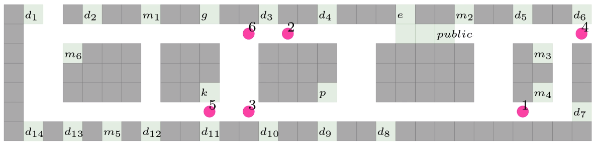
Figure 5: The office building is depicted using a grid-based layout, where areas $d_{1}$ to $d_{14}$ represent desks, $m_{1}$ to $m_{6}$ are meeting rooms, $e$ stands for the elevator, $g$ for the garbage room, $p$ for the printer room, and $k$ for the coffee kitchen. Areas marked as “public” indicate public spaces. Obstacles are illustrated in gray. The locations of robots are shown as numbered red dots.

Note that the number of segments $\ell$ might be less than the number of leaf specifications $|\Phi^{K}|$, since it is possible that not all leaf specifications are required to be satisfied, such as leaf specifications that are connected by disjunction. The following properties only apply to Alg. 2 without heuristics.

Theorem VII.6 (Completeness)

Assuming that a state-specification plan $\tau$ satisfying Asm. VII.5 exists, Alg. 2 is complete in that it is guaranteed to return a feasible state-specification plan that fulfills the hierarchical LTL specifications $\Phi$.

Proof:

The completeness of Alg. 2 is established by initially disregarding inter-spec type I switch transitions. The inclusion of type I transitions merely enlarges the search space, without impacting the algorithm’s completeness. In the absence of inter-spec type I switch transitions, only inter-spec type II switch transitions exist between team models of any two leaf specifications $\phi$ and $\phi^{\prime}$. Type II transitions connect accepting states of every PBA within the product team model of $\phi$ (or $\phi^{\prime}$) to decomposition states of the first PBA of the team model of $\phi^{\prime}$ (or $\phi$). As a result, the search does not advance to product team models of other leaf specifications until it discovers a path segment that satisfies the current leaf specification, e.g., $\phi$. Furthermore, once an accepting state of a PBA for $\phi$ is reached, the search only moves to initial states, not other decomposition states, of the first PBA in another team model, e.g., $\phi^{\prime}$, because the search on this first PBA has not started yet.

Following this logic, Alg. 2 initiates from an initial state of a certain specification $\phi$. Upon reaching one of its accepting states, the search transitions to the initial state of another specification $\phi^{\prime}$. This process is repeated until the termination condition is satisfied. Given that we employ a Dijkstra-based approach and the search within a product team model is complete as per [9], Alg. 2 is complete even without considering inter-spec type I switch transitions, thus concluding the proof. ∎

Theorem VII.7 (Optimality)

Assuming the existence of a state-specification plan $\tau^{*}$ that meets Asm. VII.5 with least cost, Alg. 2 is optimal in that the cost of the plan produced by Alg. 2 is equal to or less than the cost of $\tau^{*}$.

Proof:

To prove the optimality of Alg. 2, we first set aside inter-spec type I switch transitions. Following the same logic as in the proof of completeness, and employing a Dijkstra-based search algorithm, we can assert that searching within a product team model is optimal, as established in [9]. The addition of inter-spec type I switch transitions expands the search space, allowing for the potential discovery of a feasible plan that might not adhere to Asm. VII.5 yet could yield a lower cost. ∎

VIII Simulation Experiments

We utilizes the simulation environment described in [9], which models an office building and includes various service tasks within it. We represent this environment as a $30\times 7$ grid-based map, as depicted in Fig. 5. This map features 14 desk areas, 6 meeting rooms, and several other functional rooms. Additionally, we distribute $m$ robots at various locations within this simulated environment. Our code can be available via the https://github.com/XushengLuo92/Hierarchical-LTL-STAP.

VIII-A Scenarios

The first three scenarios are derived from the work [9]. We outline the hierarchical specifications for these scenarios below, while the corresponding flat versions of these specifications are referred to [9]. In Def. IV.2, we limit the LTL specifications to co-safe LTL. However, all hierarchical LTL specifications below contain a sub-formula expressed as $\square(a\Rightarrow b)$. Even with this sub-formula, it is still sufficient to assert satisfaction upon reaching the accepting states.

VIII-A1 Scenario 1

Empty a paper bin located at desk $d_{5}$. During this task, the robot must avoid the public area while transporting the bin.

$$L_{1}:\quad \phi({1},{1})=\Diamond\phi({2},{1})\wedge\Diamond\phi({2},{2})$$

$$L_{2}:\quad \phi({2},{1})=\Diamond(d_{5}\wedge\mathsf{default}$$

$$\quad\quad\quad\quad\wedge\bigcirc((\mathsf{carrybin}\;\mathcal{U}\;\mathsf{dispose})\wedge\Diamond\mathsf{default}))$$

$$\quad\quad\quad\quad\wedge\square(\mathsf{carrybin\Rightarrow\neg\mathsf{public}})$$

$$\phi({2},{2})=\Diamond(d_{5}\wedge\mathsf{emptybin}\wedge\bigcirc(d_{5}\wedge\mathsf{default}))$$

VIII-A2 Scenario 2

Distribute printed copies of a document to desks $d_{10}$, $d_{7}$, and $d_{5}$, and avoid public areas while carrying the document.

$$L_{1}:\quad \phi({1},{1})=\Diamond\phi({2},{1})\wedge\Diamond\phi({2},{2})\wedge\Diamond\phi({2},{3})$$

$$L_{2}:\quad \phi({2},{1})=\Diamond(p\wedge\mathsf{carry}\;\mathcal{U}\;(d_{10}\wedge\bigcirc\neg\mathsf{carry}))$$

$$\quad\quad\quad\quad\wedge\square(\mathsf{carry}\Rightarrow\neg\mathsf{public})$$

$$\phi({2},{2})=\Diamond(p\wedge\mathsf{carry}\;\mathcal{U}\;(d_{7}\wedge\bigcirc\neg\mathsf{carry}))$$

$$\quad\quad\quad\quad\wedge\square(\mathsf{carry}\Rightarrow\neg\mathsf{public})$$

$$\phi({2},{3})=\Diamond(p\wedge\mathsf{carry}\;\mathcal{U}\;(d_{5}\wedge\bigcirc\neg\mathsf{carry}))$$

$$\quad\quad\quad\quad\wedge\square(\mathsf{carry}\Rightarrow\neg\mathsf{public})$$

scenario	$t$	$t_{\text{heur}}$	$t_{\text{heur}}^{1}$	$t_{\text{heur}}^{2}$	$t_{\text{heur}}^{3}$	$c$	$c_{\text{heur}}$	$c_{\text{heur}}^{1}$	$c_{\text{heur}}^{2}$	$c_{\text{heur}}^{3}$
1	242.0$\pm$3.1	2.5$\pm$0.8	242.0$\pm$3.1	11.1$\pm$0.2	41.7$\pm$33.5	63.7$\pm$6.9	77.4$\pm$1.2	63.7$\pm$6.9	66.8$\pm$8.7	80.3$\pm$8.2
1′	232.9$\pm$18.0	2.3$\pm$0.4	93.7$\pm$14.6	20.8$\pm$6.7	27.9$\pm$20.4	81.4$\pm$8.8	82.8$\pm$6.7	82.1$\pm$6.9	82.7$\pm$9.2	82.4$\pm$9.7
2	1036.7$\pm$13.6	4.1$\pm$0.9	1036.7$\pm$13.6	46.0$\pm$1.8	21.1$\pm$13.8	91.5$\pm$6.7	98.5$\pm$5.6	91.5$\pm$6.7	94.7$\pm$ 8.6	95.4$\pm$7.2
2′	859.6$\pm$15.4	2.1$\pm$0.2	283.2$\pm$2.4	39.8$\pm$0.8	289.7$\pm$211.1	93.3$\pm$3.2	94.4$\pm$2.2	96.3$\pm$5.9	95.0$\pm$5.9	93.6$\pm$5.4
3	timeout	10.2$\pm$3.4	timeout	594.6$\pm$23.0	69.6$\pm$40.1	—	120.2$\pm$3.4	—	106.5$\pm$4.6	116.1$\pm$13.6
3′	timeout	19.1$\pm$10.4	1371.0$\pm$28.6	572.5$\pm$20.9	timeout	—	120.0$\pm$5.7	119.4$\pm$7.3	117.6$\pm$6.4	—

TABLE II: Comparison of results between methods using heuristics and those not employing heuristics. Scenarios 1^′, 2^′, and 3^′ are modifications of the first three scenarios by arranging non-leaf specifications sequentially. The symbol $t$ represents the runtime without using any heuristics. The terms $t_{\text{heur}}$, $t_{\text{heur}}^{1}$, $t_{\text{heur}}^{2}$, and $t_{\text{heur}}^{3}$ correspond to the runtimes when applying all heuristics, the heuristic of temporal order, the heuristic of essential switch transitions, and the heuristic of automaton state, respectively. This notation is similarly used for the cost, denoted as $c$.

VIII-A3 Scenario 3

Take a photo in meeting rooms $m_{1}$, $m_{4}$, and $m_{6}$. The camera should be turned off for privacy reasons when not in meeting rooms. Deliver a document from desk $d_{5}$ to $d_{3}$, ensuring it does not pass through any public areas, as the document is internal and confidential. Guide a person waiting at desk $d_{11}$ to meeting room $m_{6}$.

$$L_{1}:\quad \phi({1},{1})=\Diamond\phi({2},{1})\wedge\Diamond\phi({2},{2})\wedge\Diamond\phi({2},{3})$$

$$L_{2}:\quad \phi({2},{1})=\Diamond\phi({3},{1})\wedge\Diamond\phi({3},{2})\wedge\Diamond\phi({3},{3})$$

$$\phi({2},{2})=\Diamond(d_{5}\wedge\mathsf{carry}\;\mathcal{U}\;(d_{3}\wedge\bigcirc\neg\mathsf{carry}))$$

$$\quad\quad\quad\quad\wedge\square(\mathsf{carry}\Rightarrow\neg\mathsf{public})$$

$$\phi({2},{3})=\Diamond(d_{11}\wedge\mathsf{guide}\;\mathcal{U}\;(m_{6}\wedge\bigcirc\neg\mathsf{guide}))$$

$$L_{3}:\quad \phi({3},{1})=\Diamond(m_{1}\wedge\mathsf{photo})\wedge\square(\neg\mathsf{meeting}\Rightarrow\neg\mathsf{camera})$$

$$\phi({3},{2})=\Diamond(m_{4}\wedge\mathsf{photo})\wedge\square(\neg\mathsf{meeting}\Rightarrow\neg\mathsf{camera})$$

$$\phi({3},{3})=\Diamond(m_{6}\wedge\mathsf{photo})\wedge\square(\neg\mathsf{meeting}\Rightarrow\neg\mathsf{camera})$$

$$\mathsf{meeting}:=\;m_{1}\vee m_{2}\vee m_{3}\vee m_{4}\vee m_{5}\vee m_{6}$$

VIII-A4 Combinations of scenarios 1, 2 and 3

In addition to the individual scenarios, we examine combinations of any two of these tasks as well as the combination of all three. Due to space constraints, we only detail the scenario involving the combination of all three tasks below.

$$L_{1}:\quad \phi({1},{1})=\Diamond\phi({2},{1})\wedge\Diamond\phi({2},{2})\wedge\Diamond\phi({2},{3})$$

$$L_{2}:\quad {\color[rgb]{0,0,0}\phi({2},{1})=\Diamond\phi({3},{1})\wedge\Diamond\phi({3},{2})}$$

$${\color[rgb]{0,0,0}\phi({2},{2})=\Diamond\phi({3},{3})\wedge\Diamond\phi({3},{4})\wedge\Diamond\phi({3},{5})}$$

$${\color[rgb]{0,0,0}\phi({2},{3})=\Diamond\phi({3},{6})\wedge\Diamond\phi({3},{7})\wedge\Diamond\phi({3},{8})}$$

$$L_{3}:\quad {\color[rgb]{0,0,0}\phi({3},{1})=\Diamond(d_{5}\wedge\mathsf{default}}$$

$$\quad\quad\quad\quad{\color[rgb]{0,0,0}\wedge\bigcirc((\mathsf{carrybin}\;\mathcal{U}\;\mathsf{dispose})\wedge\Diamond\mathsf{default}))}$$

$$\quad\quad\quad\quad{\color[rgb]{0,0,0}\wedge\square(\mathsf{carrybin\Rightarrow\neg\mathsf{public}})}$$

$${\color[rgb]{0,0,0}\phi({3},{2})=\Diamond(d_{5}\wedge\mathsf{emptybin}\wedge\bigcirc(d_{5}\wedge\mathsf{default})})$$

$${\color[rgb]{0,0,0}\phi({3},{3})=\Diamond(p\wedge\mathsf{carry}\;\mathcal{U}\;(d_{10}\wedge\bigcirc\neg\mathsf{carry}))}$$

$$\quad\quad\quad\quad{\color[rgb]{0,0,0}\wedge\square(\mathsf{carry}\Rightarrow\neg\mathsf{public})}$$

$${\color[rgb]{0,0,0}\phi({3},{4})=\Diamond(p\wedge\mathsf{carry}\;\mathcal{U}\;(d_{7}\wedge\bigcirc\neg\mathsf{carry}))}$$

$$\quad\quad\quad\quad{\color[rgb]{0,0,0}\wedge\square(\mathsf{carry}\Rightarrow\neg\mathsf{public})}$$

$${\color[rgb]{0,0,0}\phi({3},{5})=\Diamond(p\wedge\mathsf{carry}\;\mathcal{U}\;(d_{5}\wedge\bigcirc\neg\mathsf{carry}))}$$

$$\quad\quad\quad\quad{\color[rgb]{0,0,0}\wedge\square(\mathsf{carry}\Rightarrow\neg\mathsf{public})}$$

$${\color[rgb]{0,0,0}\phi({3},{6})=\Diamond\phi({4},{1})\wedge\Diamond\phi({4},{2})\wedge\Diamond\phi({4},{3})}$$

$${\color[rgb]{0,0,0}\phi({3},{7})=\Diamond(d_{5}\wedge\mathsf{carry}\;\mathcal{U}\;(d_{3}\wedge\bigcirc\neg\mathsf{carry}))}$$

$$\quad\quad\quad\quad{\color[rgb]{0,0,0}\wedge\square(\mathsf{carry}\Rightarrow\neg\mathsf{public})}$$

$${\color[rgb]{0,0,0}\phi({3},{8})=\Diamond(d_{11}\wedge\mathsf{guide}\;\mathcal{U}\;(m_{6}\wedge\bigcirc\neg\mathsf{guide}))}$$

$$L_{4}:\quad {\color[rgb]{0,0,0}\phi({4},{1})=\Diamond(m_{1}\wedge\mathsf{photo})\wedge\square(\neg\mathsf{meeting}\Rightarrow\neg\mathsf{camera})}$$

$${\color[rgb]{0,0,0}\phi({4},{2})=\Diamond(m_{4}\wedge\mathsf{photo})\wedge\square(\neg\mathsf{meeting}\Rightarrow\neg\mathsf{camera})}$$

$${\color[rgb]{0,0,0}\phi({4},{3})=\Diamond(m_{6}\wedge\mathsf{photo})\wedge\square(\neg\mathsf{meeting}\Rightarrow\neg\mathsf{camera})}$$

$${\color[rgb]{0,0,0}\mathsf{meeting}:=\;m_{1}\vee m_{2}\vee m_{3}\vee m_{4}\vee m_{5}\vee m_{6}}$$

scenario	$l_{\text{flat}}$	$l_{\text{hier}}$	${\mathcal{A}}_{\text{flat}}$	${\mathcal{A}}_{\text{hier}}$	$t_{\text{flat}}$	$t_{\text{hier}}$	$c_{\text{flat}}$	$c_{\text{hier}}$
1	18	19	(17, 39)	(12, 13)	14.1$\pm$3.7	4.9$\pm$2.3	71.0$\pm$6.3	69.0$\pm$5.7
2	24	35	(56, 326)	(20, 31)	39.6$\pm$2.5	7.0$\pm$3.1	90.4$\pm$4.0	88.6$\pm$7.0
3	35	52	(180, 1749)	(30, 49)	timeout	14.5$\pm$4.1	—	97.1$\pm$5.9
1 $\wedge$ 2	43	57	(868, 12654)	(36, 49)	timeout	16.4$\pm$7.1	—	148.8$\pm$8.4
1 $\wedge$ 3	54	74	(2555, 69858)	(46, 67)	timeout	47.9$\pm$22.3	—	166.4$\pm$8.0
2 $\wedge$ 3	60	90	(6056, 325745)	(54, 85)	timeout	42.5$\pm$16.9	—	175.4$\pm$6.9
1 $\wedge$ 2 $\wedge$ 3	79	111	timeout	(70, 112)	timeout	89.6$\pm$28.1	—	246.6$\pm$8.3

TABLE III: The comparative analysis focuses on two different types of LTL specifications. We denote the lengths of the flat and hierarchical LTL specifications as $l_{\text{flat}}$ and $l_{\text{hier}}$, respectively. The sizes of the corresponding NBAs are represented by ${\mathcal{A}}_{\text{flat}}$ and ${\mathcal{A}}_{\text{hier}}$, which detail the number of nodes and edges, with the node count listed first. In terms of solutions, the runtimes for the flat and hierarchical LTL specifications are indicated by $t_{\text{flat}}$ and $t_{\text{hier}}$, respectively. Additionally, the plan horizons, or the lengths of the solutions, for the flat and hierarchical specifications are denoted by $c_{\text{flat}}$ and $c_{\text{hier}}$, respectively.

VIII-B Ablation Study on Effects of Heuristics

In the experiment, $m=2$ robots were deployed in the office environment. The results of the effects of different heuristics in scenarios 1 to 3 are detailed in Tab. II, which presents the average runtimes and cost over 20 trials per scenario. During each trial, the locations of the robots are randomly sampled within areas without labels. Our method was evaluated under three conditions: without any heuristics, with a single heuristic (either the temporal order as in Sec. VI-B1, critical switch transitions as in Sec. VI-B2, or automaton state as in Sec. VI-B3), and with the combination of all heuristics. It was observed that in scenarios 1 to 3 where non-leaf specifications have no precedence temporal order, the impact of solely using the temporal order heuristic is equivalent to not using any heuristic at all. To further investigate this, three additional scenarios were introduced where non-leaf specifications were arranged sequentially. For example, in scenario 1, $\phi(1,1)=\Diamond\phi({2},{1})\wedge\Diamond\phi({2},{2})$ was modified to $\phi(1,1)=\Diamond(\phi({2},{1})\wedge\Diamond\phi({2},{2}))$. Each navigational and manipulative action carried out incurs a cost of 1, but transitions between switches do not incur any costs. A maximum time limit of one hour was set for these tests, same as other simulations.

As expected, the method without heuristics yields solutions with minimum overall costs. However, employing all three heuristics simultaneously results in a substantial acceleration of the search process, roughly by two orders of magnitude. This significant improvement in runtimes outweighs the minor increase in costs associated with the use of heuristics. In six different scenarios, the heuristic based on essential switch transitions outperforms the other two heuristics in four scenarios. Its effectiveness is attributed to its ability to significantly reduce the number of switch transitions among team models, thus keeping the search confined within individual team models at the most time. Conversely, the temporal order heuristic is the least effective in five of the six scenarios. This inefficiency stems from the absence of precedent constraints in the non-leaf specifications of scenarios 1, 2, and 3. The cost differences between these heuristics are insignificant. In conclusion, each heuristic demonstrates improvement over the baseline method, and all of them should be applied in order to maximize the performance gain.

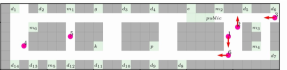
(a) $t=0$s, robots are at initial states.

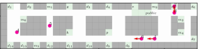
(b) $t=3$s, robot 2 arrives at desk $d_{5}$ to carry the bin.

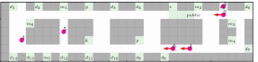
(c) $t=4$s, robot 3 arrives at desk $d_{5}$ to place the empty bin.

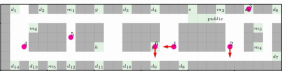
(d) $t=9$s, robot 6 arrives at printing room $p$ to pick up the document.

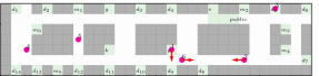
(e) $t=11$s, robot 1 arrives at printing room $p$ to pick up the document.

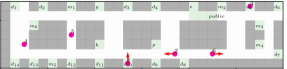
(f) $t=16$s, robot 1 arrives at desk $d_{10}$ to distribute the document.

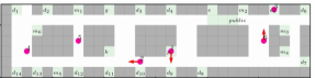
(g) $t=21$s, robot 1 arrives at printing room $p$ to pick up the document.

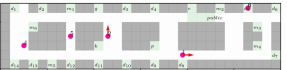
(h) $t=25$s, robot 6 arrives at desk $d_{5}$ to distribute the document.

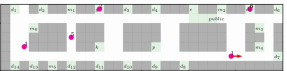
(i) $t=30$s, robot 2 arrives at garbage disposal area $g$ to dispose.

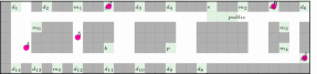
(j) $t=35$s, robot 1 arrives at desk $d_{7}$ to distribute the document.

Figure 6: The provided keyframes display the execution of the plan for the combination of scenarios 1 and 2, highlighting the completion of specific tasks. Red arrows on the robots indicate their navigation direction for the next time step. Titles of keyframes depict corresponding manipulation actions (where applicable). Note that robot 1 completes two tasks of delivering document to desks $d_{7}$ and $d_{10}$.

(a) Runtimes w.r.t number of robots

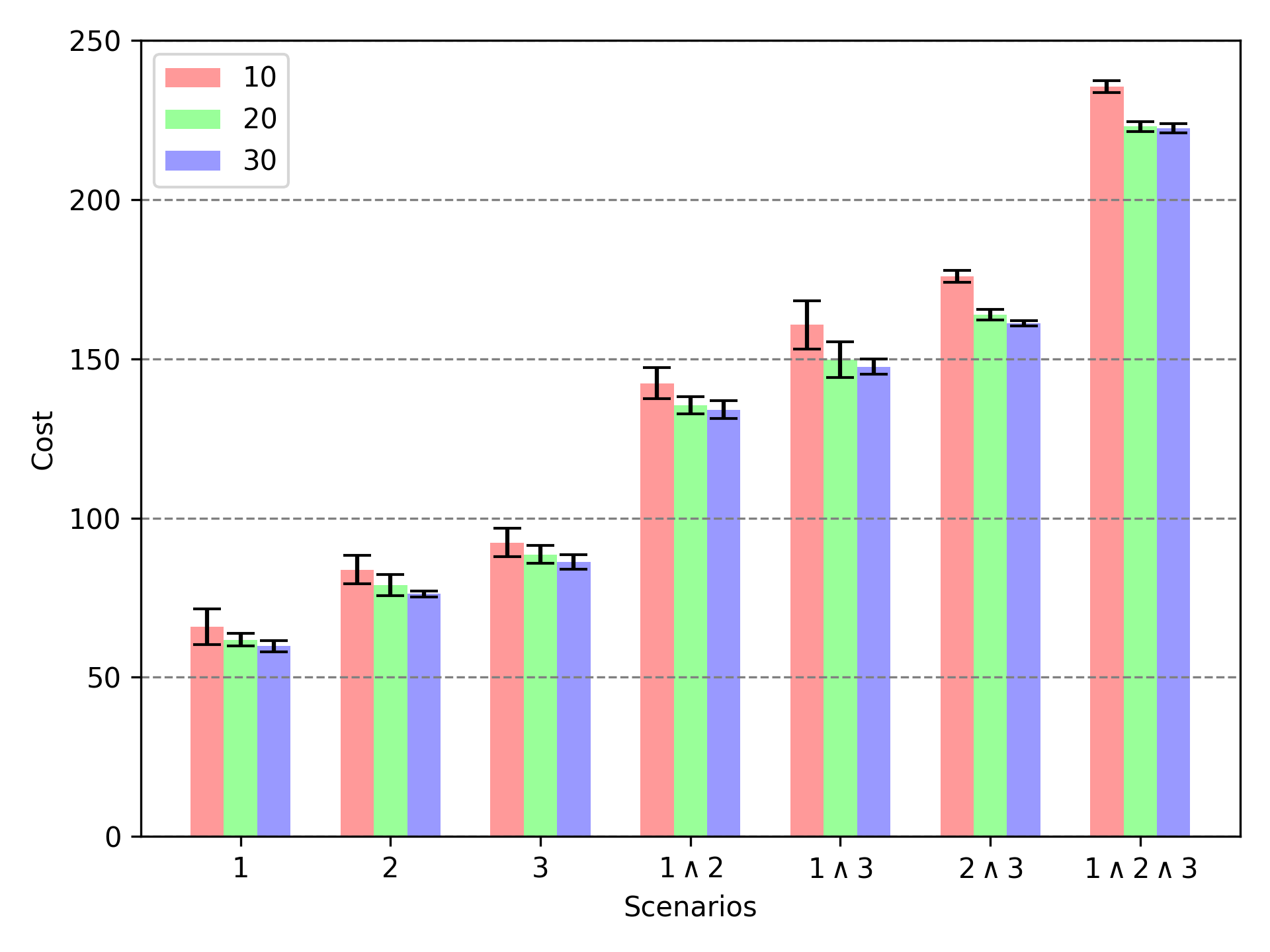
(b) Cost w.r.t number of robots

Figure 7: Scalability results of runtimes and cost w.r.t number of robots.

VIII-C Comparison with Existing Works

In our simulation, we employ $m=6$ robots within the environment and compare our method with the approach in [9], both utilizing all heuristics. It’s worth noting that Schillinger et al. [9]’s method is tailored to flat LTL specifications. Due to the absence of open-source code, we implemented their method for comparison. To the best of our knowledge, work [28] is the only existing work addressing hierarchical LTL specifications. However, it is not readily usable for mobile manipulation tasks. More importantly, Luo et al. [28] consider each transition as an individual task. In contrast, in this work tasks may consist of several transitions or even encompass the entire automaton, making each task potentially equivalent to multiple tasks as defined in [28]. Here each task is designated to be completed by a single robot, contrasting with the method in [28], where tasks could be executed collaboratively by multiple robots. This variance in task definition renders direct comparisons challenging.

Robot locations in each scenario are randomly assigned within the free space. The performance, in terms of average runtimes and costs over 20 runs, is detailed in Tab. III and includes the length of formulas and sizes of automatons. The length of a formula is the total number of logical and temporal operators. We observed that, contrary to simulation findings in [28], where hierarchical LTL shows syntactical conciseness compared to flat LTL, our hierarchical LTL specifications are longer in length. We hypothesize that the syntactical succinctness of hierarchical LTL becomes more evident in scenarios with complex interdependencies between tasks at non-bottom levels, which are more challenging to express through flat LTL specifications. This is not the case in our scenarios, where tasks at non-bottom levels are temporally independent. Upon reviewing the results, Schillinger et al. [9]’s method failed to generate solutions for the last four tasks within the one-hour limit. For tasks 1 and 2, our method produced solutions more quickly and with comparable costs. The failure of  Schillinger et al. [9]’s approach is attributed to the excessively large automatons it generates, sometimes with hundreds of thousands of edges, e.g., 325745 edges for scenario $2\wedge 3$, making the computation of the decomposition set time-consuming as it requires iterating over all possible runs. For the most complex scenario $1\wedge 2\wedge 3$, generating an automaton within one hour is impossible. In contrast, our method was able to find a solution in approximately 90 seconds. An execution plan for the combination of scenarios 1 and 2 is presented in Fig. 6.

VIII-D Scalability

For assessing scalability, we varied the number of robots from 10 to 30. The statistical findings are presented in Fig. 7. Across different scenarios, a consistent pattern emerged: as the number of robots increased, the runtimes tended to increase, while the overall costs decreased. This trend is intuitive since a greater number of robots introduces a wider range of potential solutions. In the most intricate scenario, our method was capable of identifying solutions in approximately 200 seconds, even with 30 robots.

IX Conclusion and Discussion

In this work, we address the problem of Simultaneous Task Allocation and Planning (STAP) for multiple robots subject to hierarchical LTL specifications. Our objective is to assign tasks, defined by hierarchical LTL specifications, to a group of robots and simultaneously generate their action sequences.

First, we present syntax rules for hierarchical LTL and the way to interpret its semantics, that is, verifying if hierarchical LTL specifications are satisfied by a given state-specification plan. Based on this concept of satisfaction, we develop hierarchical team models, with each model corresponding to a leaf specification. We reduce the search space by creating connections between two product team models only for states pertinent to task decomposition. To further expedite the search, we introduce several heuristics leveraging the task structure. We also provide theoretical analysis on the completeness and optimality of the proposed approach under mild assumptions.

Our simulations, focused on service tasks involving navigation and manipulation, included an ablation study on heuristics. This study demonstrated that each heuristic variably accelerates the search, with their combination yielding a significant speedup. Comparative studies with existing works illustrate that our approach can handle complex tasks beyond the reach of current methods. Additionally, scalability tests reveal our method’s capability to manage up to 30 robots within 200 seconds.

While the hierarchical LTL introduced has proven effective, there are still several areas that require additional investigation. Firstly, the automatic transforming a basic LTL into a hierarchical structure is an interesting problem to tackle. Secondly, we employ an additive cost function in this work. A potential expansion involves exploring other cost structures, such as a min-max form targeting the minimization of the makespan [68], i.e., longest individual plan, per robot. Another area of interest is addressing uncertainty in costs, which might not be predetermined. Since hierarchical LTL specifications can encompass multiple conflicting specifications, a future research avenue could be to define and maximize degree of satisfaction when all specifications cannot be concurrently met. Lastly, integrating natural languages, as in our previous work [69], to embed task hierarchies from human instructions into structured planning languages suitable for existing planners, presents an intriguing prospect.

References

- Korsah et al. [2013] G Ayorkor Korsah, Anthony Stentz, and M Bernardine Dias. A comprehensive taxonomy for multi-robot task allocation. The International Journal of Robotics Research, 32(12):1495–1512, 2013.
- LaValle [2006] Steven M LaValle. Planning algorithms. Cambridge university press, 2006.
- Woodcock et al. [2009] Jim Woodcock, Peter Gorm Larsen, Juan Bicarregui, and John Fitzgerald. Formal methods: Practice and experience. ACM computing surveys (CSUR), 41(4):1–36, 2009.
- Pnueli [1977] Amir Pnueli. The temporal logic of programs. In 18th Annual Symposium on Foundations of Computer Science (SFCS 1977), pages 46–57. ieee, 1977.
- Maler and Nickovic [2004] Oded Maler and Dejan Nickovic. Monitoring temporal properties of continuous signals. In International Symposium on Formal Techniques in Real-Time and Fault-Tolerant Systems, pages 152–166. Springer, 2004.
- Kurtz and Lin [2023] Vince Kurtz and Hai Lin. Temporal logic motion planning with convex optimization via graphs of convex sets. arXiv preprint arXiv:2301.07773, 2023.
- Tenenbaum et al. [2011] Joshua B Tenenbaum, Charles Kemp, Thomas L Griffiths, and Noah D Goodman. How to grow a mind: Statistics, structure, and abstraction. Science, 331(6022):1279–1285, 2011.
- Kemp et al. [2007] Charles Kemp, Andrew Perfors, and Joshua B Tenenbaum. Learning overhypotheses with hierarchical bayesian models. Developmental Science, 10(3):307–321, 2007.
- Schillinger et al. [2018a] Philipp Schillinger, Mathias Bürger, and Dimos V Dimarogonas. Simultaneous task allocation and planning for temporal logic goals in heterogeneous multi-robot systems. The International Journal of Robotics Research, 37(7):818–838, 2018a.
- Garrett et al. [2021] Caelan Reed Garrett, Rohan Chitnis, Rachel Holladay, Beomjoon Kim, Tom Silver, Leslie Pack Kaelbling, and Tomás Lozano-Pérez. Integrated task and motion planning. Annual review of control, robotics, and autonomous systems, 4:265–293, 2021.
- Guo and Dimarogonas [2015] Meng Guo and Dimos V Dimarogonas. Multi-agent plan reconfiguration under local LTL specifications. The International Journal of Robotics Research, 34(2):218–235, 2015.
- Tumova and Dimarogonas [2016] Jana Tumova and Dimos V Dimarogonas. Multi-agent planning under local LTL specifications and event-based synchronization. Automatica, 70:239–248, 2016.
- Yu and Dimarogonas [2021] Pian Yu and Dimos V Dimarogonas. Distributed motion coordination for multirobot systems under ltl specifications. IEEE Transactions on Robotics, 38(2):1047–1062, 2021.
- Loizou and Kyriakopoulos [December 2004] Savvas G Loizou and Kostas J Kyriakopoulos. Automatic synthesis of multi-agent motion tasks based on LTL specifications. In 43rd IEEE Conference on Decision and Control (CDC), volume 1, pages 153–158, The Bahamas, December 2004.
- Smith et al. [2011] Stephen L Smith, Jana Tůmová, Calin Belta, and Daniela Rus. Optimal path planning for surveillance with temporal-logic constraints. The International Journal of Robotics Research, 30(14):1695–1708, 2011.
- Saha et al. [2014] Indranil Saha, Rattanachai Ramaithitima, Vijay Kumar, George J Pappas, and Sanjit A Seshia. Automated composition of motion primitives for multi-robot systems from safe LTL specifications. In 2014 IEEE/RSJ International Conference on Intelligent Robots and Systems, pages 1525–1532. IEEE, 2014.
- Kantaros and Zavlanos [2017] Yiannis Kantaros and Michael M Zavlanos. Sampling-based control synthesis for multi-robot systems under global temporal specifications. In 2017 ACM/IEEE 8th International Conference on Cyber-Physical Systems (ICCPS), pages 3–14. IEEE, 2017.
- Kantaros and Zavlanos [2018a] Yiannis Kantaros and Michael M Zavlanos. Distributed optimal control synthesis for multi-robot systems under global temporal tasks. In Proceedings of the 9th ACM/IEEE International Conference on Cyber-Physical Systems, pages 162–173. IEEE Press, 2018a.
- Kantaros and Zavlanos [2018b] Yiannis Kantaros and Michael M Zavlanos. Sampling-based optimal control synthesis for multirobot systems under global temporal tasks. IEEE Transactions on Automatic Control, 64(5):1916–1931, 2018b.
- Kantaros and Zavlanos [2020] Yiannis Kantaros and Michael M Zavlanos. Stylus*: A temporal logic optimal control synthesis algorithm for large-scale multi-robot systems. The International Journal of Robotics Research, 39(7):812–836, 2020.
- Kantaros et al. [2022] Yiannis Kantaros, Samarth Kalluraya, Qi Jin, and George J Pappas. Perception-based temporal logic planning in uncertain semantic maps. IEEE Transactions on Robotics, 38(4):2536–2556, 2022.
- Luo and Zavlanos [2019] Xusheng Luo and Michael M Zavlanos. Transfer planning for temporal logic tasks. In 2019 IEEE 58th Conference on Decision and Control (CDC), pages 5306–5311. IEEE, 2019.
- Luo et al. [2021] Xusheng Luo, Yiannis Kantaros, and Michael M Zavlanos. An abstraction-free method for multirobot temporal logic optimal control synthesis. IEEE Transactions on Robotics, 37(5):1487–1507, 2021.
- Kloetzer et al. [2011] Marius Kloetzer, Xu Chu Ding, and Calin Belta. Multi-robot deployment from LTL specifications with reduced communication. In 2011 50th IEEE Conference on Decision and Control and European Control Conference, pages 4867–4872. IEEE, 2011.
- Shoukry et al. [2017] Yasser Shoukry, Pierluigi Nuzzo, Ayca Balkan, Indranil Saha, Alberto L Sangiovanni-Vincentelli, Sanjit A Seshia, George J Pappas, and Paulo Tabuada. Linear temporal logic motion planning for teams of underactuated robots using satisfiability modulo convex programming. In 2017 IEEE 56th Annual Conference on Decision and Control (CDC), pages 1132–1137. IEEE, 2017.
- Moarref and Kress-Gazit [2017] Salar Moarref and Hadas Kress-Gazit. Decentralized control of robotic swarms from high-level temporal logic specifications. In 2017 International Symposium on Multi-robot and Multi-agent Systems (MRS), pages 17–23. IEEE, 2017.
- Lacerda and Lima [2019] Bruno Lacerda and Pedro U Lima. Petri net based multi-robot task coordination from temporal logic specifications. Robotics and Autonomous Systems, 122:103289, 2019.
- Luo et al. [2023a] Xusheng Luo, Shaojun Xu, Ruixuan Liu, and Changliu Liu. Decomposition-based hierarchical task allocation and planning for multi-robots under hierarchical temporal logic specifications. arXiv preprint arXiv:2308.10393, 2023a.
- Sahin et al. [2019] Yunus Emre Sahin, Petter Nilsson, and Necmiye Ozay. Multirobot coordination with counting temporal logics. IEEE Transactions on Robotics, 2019.
- Djeumou et al. [2020] Franck Djeumou, Zhe Xu, and Ufuk Topcu. Probabilistic swarm guidance subject to graph temporal logic specifications. In Robotics: Science and Systems, 2020.
- Yan et al. [2019] Ruixuan Yan, Zhe Xu, and Agung Julius. Swarm signal temporal logic inference for swarm behavior analysis. IEEE Robotics and Automation Letters, 4(3):3021–3028, 2019.
- Leahy et al. [2021] Kevin Leahy, Zachary Serlin, Cristian-Ioan Vasile, Andrew Schoer, Austin M Jones, Roberto Tron, and Calin Belta. Scalable and robust algorithms for task-based coordination from high-level specifications (scratches). IEEE Transactions on Robotics, 38(4):2516–2535, 2021.
- Luo and Zavlanos [2022] Xusheng Luo and Michael M Zavlanos. Temporal logic task allocation in heterogeneous multirobot systems. IEEE Transactions on Robotics, 38(6):3602–3621, 2022.
- Liu et al. [2022] Zesen Liu, Meng Guo, and Zhongkui Li. Time minimization and online synchronization for multi-agent systems under collaborative temporal tasks. arXiv preprint arXiv:2208.07756, 2022.
- Li et al. [2023] Lin Li, Ziyang Chen, Hao Wang, and Zhen Kan. Fast task allocation of heterogeneous robots with temporal logic and inter-task constraints. IEEE Robotics and Automation Letters, 2023.
- Camacho et al. [2017] Alberto Camacho, Eleni Triantafillou, Christian J Muise, Jorge A Baier, and Sheila A McIlraith. Non-deterministic planning with temporally extended goals: Ltl over finite and infinite traces. In AAAI, pages 3716–3724, 2017.
- Camacho et al. [2019] Alberto Camacho, R Toro Icarte, Toryn Q Klassen, Richard Valenzano, and Sheila A McIlraith. LTL and beyond: Formal languages for reward function specification in reinforcement learning. In Proceedings of the 28th International Joint Conference on Artificial Intelligence (IJCAI), pages 6065–6073, 2019.
- Schillinger et al. [2019] Philipp Schillinger, Mathias Bürger, and Dimos V Dimarogonas. Hierarchical LTL-task mdps for multi-agent coordination through auctioning and learning. The International Journal of Robotics Research, 2019.
- Liu et al. [2024] Zesen Liu, Meng Guo, and Zhongkui Li. Time minimization and online synchronization for multi-agent systems under collaborative temporal logic tasks. Automatica, 159:111377, 2024.
- Biere et al. [2006] Armin Biere, Keijo Heljanko, Tommi Junttila, Timo Latvala, and Viktor Schuppan. Linear encodings of bounded LTL model checking. Logical Methods in Computer Science, 2(5:5):1–64, 2006.
- Leahy et al. [2022] Kevin Leahy, Austin Jones, and Cristian-Ioan Vasile. Fast decomposition of temporal logic specifications for heterogeneous teams. IEEE Robotics and Automation Letters, 7(2):2297–2304, 2022.
- Schillinger et al. [2018b] Philipp Schillinger, Mathias Bürger, and Dimos V Dimarogonas. Decomposition of finite LTL specifications for efficient multi-agent planning. In Distributed Autonomous Robotic Systems, pages 253–267. Springer, 2018b.
- Faruq et al. [2018] Fatma Faruq, David Parker, Bruno Laccrda, and Nick Hawes. Simultaneous task allocation and planning under uncertainty. In 2018 IEEE/RSJ International Conference on Intelligent Robots and Systems (IROS), pages 3559–3564. IEEE, 2018.
- Robinson et al. [2021] Thomas Robinson, Guoxin Su, and Minjie Zhang. Multiagent task allocation and planning with multi-objective requirements. In Proceedings of the 20th International Conference on Autonomous Agents and MultiAgent Systems, pages 1628–1630, 2021.
- Okumura and Défago [2023] Keisuke Okumura and Xavier Défago. Solving simultaneous target assignment and path planning efficiently with time-independent execution. Artificial Intelligence, 321:103946, 2023.
- Liu et al. [2021] Zhe Liu, Huanshu Wei, Hongye Wang, Haoang Li, and Hesheng Wang. Integrated task allocation and path coordination for large-scale robot networks with uncertainties. IEEE Transactions on Automation Science and Engineering, 19(4):2750–2761, 2021.
- Edison and Shima [2011] Eugene Edison and Tal Shima. Integrated task assignment and path optimization for cooperating uninhabited aerial vehicles using genetic algorithms. Computers & Operations Research, 38(1):340–356, 2011.
- Chen et al. [2021] Zhe Chen, Javier Alonso-Mora, Xiaoshan Bai, Daniel D Harabor, and Peter J Stuckey. Integrated task assignment and path planning for capacitated multi-agent pickup and delivery. IEEE Robotics and Automation Letters, 6(3):5816–5823, 2021.
- Aggarwal et al. [2022] Aayush Aggarwal, Florence Ho, and Shinji Nakadai. Extended time dependent vehicle routing problem for joint task allocation and path planning in shared space. In 2022 IEEE/RSJ International Conference on Intelligent Robots and Systems (IROS), pages 12037–12044. IEEE, 2022.
- Ma and Koenig [2016] Hang Ma and Sven Koenig. Optimal target assignment and path finding for teams of agents. In Proceedings of the 2016 International Conference on Autonomous Agents & Multiagent Systems, pages 1144–1152, 2016.
- Guo et al. [2023] Huihui Guo, Fan Wu, Yunchuan Qin, Ruihui Li, Keqin Li, and Kenli Li. Recent trends in task and motion planning for robotics: A survey. ACM Computing Surveys, 2023.
- Motes et al. [2020] James Motes, Read Sandström, Hannah Lee, Shawna Thomas, and Nancy M Amato. Multi-robot task and motion planning with subtask dependencies. IEEE Robotics and Automation Letters, 5(2):3338–3345, 2020.
- Zhang et al. [2022] Hejia Zhang, Shao-Hung Chan, Jie Zhong, Jiaoyang Li, Sven Koenig, and Stefanos Nikolaidis. A mip-based approach for multi-robot geometric task-and-motion planning. In 2022 IEEE 18th International Conference on Automation Science and Engineering (CASE), pages 2102–2109. IEEE, 2022.
- Motes et al. [2023] James Motes, Tan Chen, Timothy Bretl, Marco Morales Aguirre, and Nancy M Amato. Hypergraph-based multi-robot task and motion planning. IEEE Transactions on Robotics, 2023.
- Pan et al. [2021] Tianyang Pan, Andrew M Wells, Rahul Shome, and Lydia E Kavraki. A general task and motion planning framework for multiple manipulators. In 2021 IEEE/RSJ International Conference on Intelligent Robots and Systems (IROS), pages 3168–3174. IEEE, 2021.
- Toussaint [2015] Marc Toussaint. Logic-geometric programming: An optimization-based approach to combined task and motion planning. In IJCAI, pages 1930–1936, 2015.
- [57] Jimmy Envall, Roi Poranne, and Stelian Coros. Differentiable task assignment and motion planning.
- Wilkins [2014] David E Wilkins. Practical planning: extending the classical AI planning paradigm. Elsevier, 2014.
- Georgievski and Aiello [2015] Ilche Georgievski and Marco Aiello. Htn planning: Overview, comparison, and beyond. Artificial Intelligence, 222:124–156, 2015.
- Weser et al. [2010] Martin Weser, Dominik Off, and Jianwei Zhang. Htn robot planning in partially observable dynamic environments. In 2010 IEEE International Conference on Robotics and Automation, pages 1505–1510. IEEE, 2010.
- De Mello and Sanderson [1990] LS Homem De Mello and Arthur C Sanderson. And/or graph representation of assembly plans. IEEE Transactions on robotics and automation, 6(2):188–199, 1990.
- Cheng et al. [2021] Yujiao Cheng, Liting Sun, and Masayoshi Tomizuka. Human-aware robot task planning based on a hierarchical task model. IEEE Robotics and Automation Letters, 6(2):1136–1143, 2021.
- Baier and McIlraith [2009] SSJA Baier and Sheila A McIlraith. Htn planning with preferences. In 21st Int. Joint Conf. on Artificial Intelligence, pages 1790–1797, 2009.
- Lin and Bercher [2022] Songtuan Lin and Pascal Bercher. On the expressive power of planning formalisms in conjunction with ltl. In Proceedings of the International Conference on Automated Planning and Scheduling, volume 32, pages 231–240, 2022.
- Baier and Katoen [2008] Christel Baier and Joost-Pieter Katoen. Principles of model checking. MIT press Cambridge, 2008.
- Vardi and Wolper [1986] Moshe Y Vardi and Pierre Wolper. An automata-theoretic approach to automatic program verification. In 1st Symposium in Logic in Computer Science (LICS). IEEE Computer Society, 1986.
- Kupferman and Vardi [2001] Orna Kupferman and Moshe Y Vardi. Model checking of safety properties. Formal Methods in System Design, 19(3):291–314, 2001.
- Yu and LaValle [2016] Jingjin Yu and Steven M LaValle. Optimal multirobot path planning on graphs: Complete algorithms and effective heuristics. IEEE Transactions on Robotics, 32(5):1163–1177, 2016.
- Luo et al. [2023b] Xusheng Luo, Shaojun Xu, and Changliu Liu. Obtaining hierarchy from human instructions: an llms-based approach. In CoRL 2023 Workshop on Learning Effective Abstractions for Planning (LEAP), 2023b.