BST1047+1156: A (Failing) Ultradiffuse Tidal Dwarf in the Leo I Group

Abstract

We use deep Hubble Space Telescope imaging to study the resolved stellar populations in BST1047+1156, a gas-rich, ultradiffuse dwarf galaxy found in the intragroup environment of the Leo I galaxy group. While our imaging reaches approximately two magnitudes below the tip of the red giant branch at the Leo I distance of 11 Mpc, we find no evidence for an old red giant sequence that would signal an extended star formation history for the object. Instead, we clearly detect the red and blue helium burning sequences of its stellar populations, as well as the fainter blue main sequence, all indicative of a recent burst of star formation having taken place over the past 50–250 Myr. Comparing to isochrones for young metal-poor stellar populations, we infer this post-starburst population to be moderately metal poor, with metallicity [M/H] in the range $-1$ to $-1.5$. The combination of a young, moderately metal-poor post starburst population and no old stars motivates a scenario in which BST1047 was recently formed during a weak burst of star formation in gas that was tidally stripped from the outskirts of the neighboring massive spiral M96. BST1047’s extremely diffuse nature, lack of ongoing star formation, and disturbed HI morphology all argue that it is a transitory object, a “failing tidal dwarf” in the process of being disrupted by interactions within the Leo I group. Finally, in the environment surrounding BST1047, our imaging also reveals the old, metal-poor ([M/H]$=-1.3\pm 0.2$) stellar halo of M96 at a projected radius of 50 kpc.

1 Introduction

The properties of extreme low surface brightness (LSB) galaxies continue to challenge models of galaxy formation and evolution. While much attention has been focused recently on the “ultra-diffuse galaxies” found in dense galaxy clusters, gas-rich LSBs found in the field and group environments (e.g.,  McGaugh & Bothun, 1994; Cannon et al., 2015; Leisman et al., 2017) may have a less complicated evolutionary path, and better probe mechanisms driving galaxy formation at the lowest densities. For example, the high gas fractions and low metallicities of LSB galaxies (McGaugh & Bothun, 1994; Ellison et al., 2008; Pilyugin et al., 2014) argue that they have converted little of their baryonic mass into stars. This is likely due to their extremely low gas densities (van der Hulst et al., 1993; van Zee et al., 1997; Wyder et al., 2009), which result in a sputtering and inefficient star formation history (Schombert et al., 2001; Schombert & McGaugh, 2014, 2015). Thus, these galaxies raise questions both macro and micro: how galaxy formation is linked to the global environment, and how stars form on smaller scales within galaxies.

The recent discovery of the extreme LSB galaxy BST1047+1156 (Mihos et al., 2018, hereafter BST1047) is particularly notable in this context. With an HI velocity that places it unambiguously within the Leo I galaxy group (D=11 Mpc; Graham et al., 1997; Lee & Jang, 2016), BST1047 has the lowest surface brightness of any known star forming galaxy ($\mu_{B,peak}$=28.8 mag arcsec^-2), an isophotal radius of $R_{30}\approx$ 2 kpc, and a total gas mass of $4.5\times 10^{7}$ $M_{\odot}$(Mihos et al., 2018). The object’s peak HI column density ($1.4\times 10^{20}\ {\rm cm}^{-2}$) is well below that in which stars typically form (Bigiel et al., 2008, 2010; Krumholz et al., 2009; Clark & Glover, 2014), yet its extremely blue optical colors ($B-V=0.14\pm 0.09$) and GALEX far-UV emission both argue for the presence of young stars (Mihos et al., 2018). BST1047’s combination of extraordinarily high gas fraction ($f_{g}\approx 0.99$), extremely blue optical colors, and vanishingly low surface brightness makes it the most extreme gas-rich LSB object known to date.

Exactly how BST1047 formed, and what has triggered its recent star formation, remains unclear. The Leo I group is awash in extended HI, including the large “Leo HI Ring” surrounding NGC 3379 to the north (Schneider, 1985; Schneider et al., 1986), likely a remnant of past tidal interactions (Michel-Dansac et al., 2010; Corbelli et al., 2021). BST1047 itself is embedded in a low density HI stream connecting the Ring to the spiral galaxy M96. This, plus the fact that BST1047 sports a pair of HI tidal tails of its own, suggests the object may be an extremely diffuse LSB galaxy recovering from a weak burst of tidally-triggered star formation. Alternatively, BST1047 may be a “tidal dwarf galaxy,” (e.g.,  Duc et al., 2000; Lelli et al., 2015), spawned directly from tidally compressed gas, with the young stars marking its formation age. Since tidal dwarfs should be free of dark matter (Barnes & Hernquist, 1992; Elmegreen et al., 1993) and perhaps only tenuously bound, under this scenario BST1047 may be a short-lived object — a “failing” tidal dwarf caught in the throes of tidal disruption in the group environment.

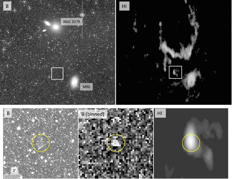
Figure 1: Optical and HI imaging of the Leo I Group and BST1047+1156, taken from Mihos et al. (2018). The upper left panel shows the deep wide-field B-band imaging of Watkins et al. (2014), while the upper right panel shows the HI map from Oosterloo et al. (2010). In these panels, the white box shows the location of BST1047 in the Leo I group, and is blown up in the lower panels. The lower left panel shows the B-band image, while the lower center panel shows the B-image after being masked of compact sources and rebinned in 9$\times$9 pixel boxes to show low surface brightness emission. The lower right panel shows the HI map on the same scale. In the lower panels, the yellow circle is 70″ in radius, twice the size of the $R_{30}$ isophote.

Either of these scenarios has important ramifications for issues surrounding theories of formation and evolution of low mass galaxies. If BST1047 is a diffuse but long-lived LSB galaxy, with an established, old stellar population, it challenges star formation models which posit that stars should not form at such low gas densities. Under such models, where has the older population come from? How can galaxies this diffuse sustain such prolonged star formation histories? Conversely, if BST1047 is a disrupting tidal dwarf, it would provide insight into the evolutionary link between tidal interactions, formation and disruption of dwarf galaxies, and the deposition of young stars into the intragroup medium. Key to resolving the question of BST1047’s origin is an understanding of its stellar populations — in particular, does it have a well established old red giant branch sequence, indicative of an long-lived star forming history, or are the stellar populations exclusively young, as might be expected BST1047 was recently formed during a tidal encounter?

To answer these questions, we use deep Hubble Space Telescope ACS imaging to study the stellar populations of BST1047. Using the F606W and F814W filters, our imaging extends roughly two magnitudes below the expected tip of the red giant branch at the Leo I distance, allowing us to detect and characterize stellar populations across a range of ages, including any red giant branch stars, red and blue helium burning stars, and potentially even upper main sequence stars. These various populations give constraints on the ages and the metallicities of both young and old stellar populations, providing strong constraints on the extended star formation history in BST1047.

2 Observational Data

2.1 Imaging and Reduction

We imaged BST1047 using the Wide Field Channel (WFC) of the Advanced Camera for Surveys (ACS) on the Hubble Space Telescope (HST) under program GO-16762. The imaging field, shown in the left panel of Figure 2, places BST1047 in the eastern side of the ACS field of view, avoiding nearby bright stars and leaving the western side blank for background estimation.

The field was imaged over 8 orbits in F606W and 7 orbits in F814W; each orbit consisted of two 1185s exposures, yielding total exposure times of 16458s and 16590s in F606W and F814W, respectively (one F606W exposure was cut short due to guide star loss). Each visit made use of a small ($\sim$ 3.5–4.5 pixel) custom four point box dither pattern to aid in sub-pixel sampling of the ACS images and to also avoid placing any objects on bad or hot pixels. The different visits were further shifted in slightly larger (20 pixel) offsets to avoid other artifacts and facilitate effective cosmic ray removal in our long (1/2 orbit) exposures. As BST1047 is small enough to fit into a single WFC chip, the galaxy was centered on the WFC1 chip, and no attempt was made to cover the ACS chip gap.

Point-source photometry is carried out on the individual, CTE-corrected flc images using DOLPHOT (described below), which requires a sufficiently deep drizzled image to use as an astrometric reference. To create this image, the individual images from different visits needed to be precisely aligned. We found that images from the three visits (including eight F606W images and two F814W images) that were astrometrically calibrated with the GSC v2.4.2 catalog were slightly offset ($\sim 0.5$pixel in F606W; $\sim 0.2$pixels in F814W) from the remaining 20 images calibrated to the newer Gaia eDR3 catalog. To improve the relative image alignments, we used the drizzlepac/tweakreg package to adjust the image world coordinate systems based on point source positions on the individual flc images measured using Source-Extractor (Bertin & Arnouts, 1996). After these corrections, we used drizzlepac/astrodrizzle to create stacked deep F606W and F814W images of the ACS field; the F814W image is shown in the left panel of Figure 2.

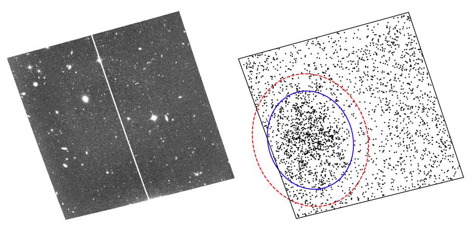
Figure 2: Left panel: Stacked F814W ACS image of BST1047+1156, with a total exposure time of 14$\times$1215s. North is up, east is to the left, and the field of view is 202″$\times$202″. Right panel: Spatial distribution of point sources detected in the ACS imaging. All point sources within the solid blue ellipse are used for the analysis of BST1047, while point sources found outside the dashed red ellipse are considered part of the background or surrounding environment.

2.2 Point Source Photometry and Artificial Star Tests

With such an extremely low surface brightness ($\langle\mu_{B}\rangle_{e}=28.9$ mag arcsec^-2; Mihos et al., 2018), the integrated light from BST1047 is too faint to show up unambiguously in our ACS imaging; instead, we only detect it through its resolved stellar populations. We use the software package DOLPHOT (an updated version of HSTPhot; Dolphin, 2000) to perform point-source photometry of objects on the individual CTE-corrected flc images using pre-computed Tiny Tim PSFs (Krist, 1995). We performed object detection and photometry on all 30 individual images (16 in F606W; 14 in F814W) images simultaneously, using the deep F814W drizzled image stack created above for the reference image. We used the Nov 2019 version of DOLPHOT 2.0 (available at http://americano.dolphinsim.com/dolphot/) to pre-process the raw flc images, applying bad-pixel masks and pixel-area masks (acsmask), splitting the images into the individual WFC1/2 chip images (splitgroups), and constructing an initial background sky map for each chip/image from each image (calcsky).

Photometry with DOLPHOT is very dependent on the choice of input parameters (see Williams et al., 2014), so we experimented with a number of the parameters, finally settling on values similar to those used in previous deep photometric studies with ACS (e.g.,  Williams et al., 2014; Mihos et al., 2018; Shen et al., 2021) and/or suggested by the DOLPHOT/ACS User’s Guide. As our ACS field is relatively uncrowded, we adopted a photometric aperture RAper=4.0 pix, a PSF fitting region of RPSF=10 pix, and the FITSKY=1 option for derivation of the sky background The only changes we made to the usual DOLPHOT workflow were the derivation of the aperture corrections on each chip/image. With so few bright stellar objects in our frames, some of the individual DOLPHOT-computed aperture corrections (and thus the individual F606W/F814W magnitudes) could be affected, even for brighter stars. To improve this, we input our own visually-selected list of 53 isolated stellar objects over the entire field which DOLPHOT could use to compute aperture corrections. The final aperture corrections for each chip/image/filter were based on anywhere from 6 to 29 measured stars. Finally, the instrumental magnitudes were converted to the VEGAMAG HST photometric system. We used updated zeropoints (at the time of observations, using the ACS zeropoint calculator (https://acszeropoints.stsci.edu/) of 26.398 for F606W and 25.502 for F814W. We present all photometry in the VEGAMAG system unless explicitly stated otherwise.

To ensure the most accurate point source photometry, we apply the following selection parameters to the photometric catalog. We start by selecting only those objects with DOLPHOT object TYPE=1 (“good star”) and signal-to-noise S/N$>$3.5 in both the F606W and F814W filters. We also only select sources that are uncrowded (CROWD$<$0.25) and have a goodness of fit value of CHI$<$2.4 in both filters; these values are based both on visual inspection of bright stars and galaxies in our images, and the results from the artificial stars detailed below. At fainter magnitudes (F814W$>$26), contamination from unresolved background galaxies becomes problematic. To reduce this contamination, we also make a magnitude-dependent cut on the DOLPHOT SHARP parameter, using $|SHARP|<0.04+0.3e^{(m-m_{\rm crit})}$, with $m_{\rm crit}=$ 29.5 and 28.7 in F606W and F814W, respectively. This function is similar to that used in the our previous HST studies of stellar populations in M101 and the Virgo Cluster (Mihos et al., 2018, 2022), and the function parameters are chosen based both on the observed photometric catalog and on our artificial star analysis. We have also checked that the sources rejected under our SHARP criteria do not show stellar population-like patterns in the color-magnitude diagram that might suggest we are over-aggressively rejecting actual stars in the Leo I group environment. The spatial distribution of point sources selected in this fashion are shown in the right panel of Figure 2.

To assess the photometric completeness and bias of the photometry in our ACS imaging, we use DOLPHOT to insert and measure 100,000 artificial stars over the magnitude range $22<{\rm F606W}<30$ and color range $-0.5<{\rm F606W-F814W}<2.0$. We process the artificial stars using the same photometric selection criteria used for the actual data, and plot in Figure 3 the completeness fraction and shift in magnitude and color (defined as input minus measured) as a function of F814W magnitude and F606W$-$F814W color. Because of our joint selection in F606W and F814W, completeness is a function of both magnitude and color, with 50% completeness at F814W=28.2 in the blue (at F606W$-$F814W=0.0), and rising to F814W=27.8 in the red (at F606W$-$F814W=1.0). At magnitudes brighter than F814W=27.0 we see little systematic shift in either magnitude or color, but at fainter magnitudes shifts in both are evident at the $\approx$ 0.1 mag level, consistent with our previous analysis of ACS data in Mihos et al. (2018). In our analysis that follows, we always plot magnitudes and colors as measured, correcting only for foreground extinction ($A_{\rm F606W}=0.062,A_{\rm F814W}=0.038$, Schlafly & Finkbeiner, 2011), and use the results of the artificial star tests to adjust the theoretical stellar isochrones to account for these systematic effects when interpreting our photometric results.

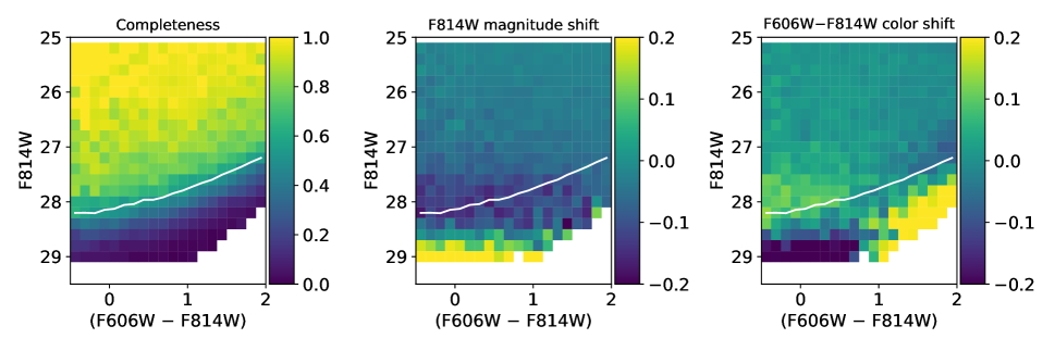
Figure 3: Results of artificial star tests. Left panel: Completeness, Middle panel: F814W magnitude shift, Right panel: F606W$-$F814W color shift. Shifts are measured as input minus measured values, such that a positive magnitude shift corresponds to a star being measured systematically too bright, and a positive color shift corresponds to a star being measured systematically too blue. In each panel, the white line shows the 50% completeness limit.

3 Analysis

The right panel of Figure 2 shows the spatial distribution of point sources in our ACS field; an excess of sources corresponding to the stellar population of BST1047 can clearly be seen on the eastern half of the FOV. The distribution of point sources appears slightly elongated roughly along the north-south axis, and shows small scale clumpiness as well. We construct a color-magnitude diagram (CMD) for BST1047 by extracting all point sources within an ellipse (determined by eye and shown in Figure 2) centered at $(\alpha,\delta)_{J2000}$=(10:47:43.59, 11:55:47.0), and having an ellipticity of 0.85, semimajor axis of 50″, and position angle of 17°. The center of this ellipse is approximately 14.3″ south of BST1047’s center coordinate originally reported in Mihos et al. (2018). For comparison, we also construct a background CMD by extracting sources that lie outside a 350 pixel (17.5″) buffer around the BST1047 ellipse, shown as the dotted red ellipse in Figure 2. The extracted CMDs for each region (BST1047 and background) are shown in the top panels of Figure 4.

While the background region is meant as a control for the BST1047 field, it has a much larger area (by a factor of 2.87), and thus over-represents the potential contamination to BST1047’s CMD. The lower right panel corrects for this difference in area by randomly subsampling sources in the background region by a factor of 2.87 to match the area of the BST1047 field, thus acting as a more representative control sample for BST1047.

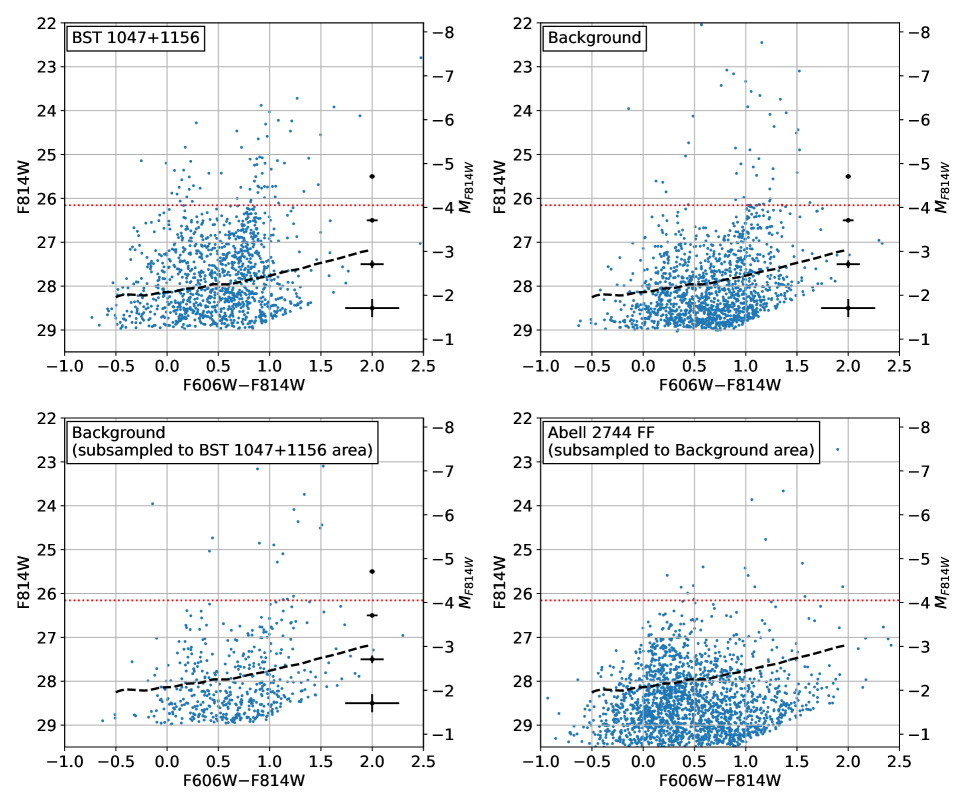
Figure 4: Color-magnitude diagrams for point sources in the ACS imaging. The top panels shows the extracted CMDs for BST1047 (left) and the background (right). The lower left panel shows the background CMD randomly subsampled to match the area of BST1047, while the lower right panel shows the point source CMD for the Abell 2744 Flanking Field data (taken from the analysis of Mihos et al. 2018), randomly subsampled to match the area of the background field. Each CMD in the lower panels thus acts as a control field for the CMD immediately above it. In each subpanel, the right axis shows the apparent magnitude, the left axis shows the absolute magnitude at the adopted 11.0 Mpc distance of the Leo I Group, and the red dotted line shows the expected RGB tip magnitude. Typical errorbars as a function of magnitude are shown in black, and the 50% completeness limit for the BST1047 imaging is shown as the dashed black line.

Of course, the background region itself is not a pure background. As BST1047 resides within the Leo I group, and also sits projected only 15′ (48 kpc) northeast of the luminous spiral galaxy M96, our ACS pointing samples not only background sources, but also stars in M96’s extended stellar halo, as well as any potential Leo I intragroup stars (Watkins et al., 2014; Ragusa et al., 2022). To estimate a cleaner background CMD, we turn to the deep HST imaging of the Abell 2744 Flanking Field (Lotz et al., 2017). That imaging used the same filters used here, and in Mihos et al. (2018) we extracted point source photometry for that imaging using the same techniques as described above. Thus, it acts as a reasonable control field for our background region here. In the lower right panel of Figure 4 we show the Abell 2744 Flanking Field photometry, using the same selection criteria as used in this study, and subsampled down by a factor of 1.62 to match the area of our background region.

We start with a discussion of the CMD in the full background region (upper right panel of Figure 4), comparing it to its control field, the subsampled Abell 2744 FF field directly below it. The most striking feature of the background region is the clear signature of a metal-poor red giant branch population, terminating at the expected RGB tip at F814W=26.2. Brighter than this, there are a number of red stars in the field, possibly AGB stars or true background contaminants. At these magnitudes, and over the small ACS field of view, foreground contamination from Milky Way stars should be small; comparing to the TRILEGAL models of Girardi et al. (2005); Girardi (2016) we would expect only a handful of objects brighter than the observed RGB tip. At fainter magnitudes (F814W$>$26) we also see a swarm of bluer sources with colors $0.0<{\rm F606W-F814W}<0.5$, but these sources appear comparable in number to those seen in the Abell 2744 Flanking Field, and are likely unresolved background sources. Finally, we also see a handful of brighter sources in this bluer color range, but not obviously in excess of the background expectation.

Turning to the CMD for BST1047 itself, we again see a clear red sequence of stars, but one that is distinctly bluer than that in the background region. Whereas the sequence in the background region reaches a color of F606W$-$F814W$\approx$1.03 when it reaches the RGB tip, the sequence in BST1047 has a color of F606W$-$F814W$\approx$0.78 at a comparable brightness, and continues on to brighter magnitudes above the expectation for the RGB tip.

We demonstrate this color difference in Figure 5, which shows the color distribution of point sources of all colors, in the magnitude range $m_{\rm tip}\leq{\rm F814W}\leq m_{\rm tip}+0.75$ (i.e., within 0.75 magnitudes of the expected RGB tip). The left panel shows the relative color distribution in each region, where the color difference between the red sequences in each region is clear. The right panel of Figure 5 shows the surface density of sources as a function of color – in other words, the color distribution normalized by area. Here too, the difference in the red sequences is dramatic: not only are they different in color, the density of red stars is much higher in BST1047 than in the background. The two sequences are clearly tracing different populations of stars.

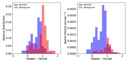
Figure 5: Color distribution of point sources in the magnitude range $m_{\rm tip,F814W}<{\rm F814W}<m_{\rm tip,F814W}+0.75$. The left panel shows the relative fraction of sources in each field, while the right panel shows the actual number density of sources.

At magnitudes brighter than the RGB tip, the CMDs in Figure 4 show an excess of stars in BST1047 both at red colors (F606W$-$F814W $\approx$ 0.8–1.0) and in the blue (F606W$-$F814W $\approx$ 0.0–0.4) compared to the background region. The morphology and color of these bright red and blue sequences suggest they are helium burning sequences from evolving massive stars, signatures of recent star formation in BST1047. At fainter magnitudes (F814W $\sim$ 26–28) we also see an excess population of stars with very blue colors of F606W$-$F814W $<$ 0.0 compared to the background. These sources can also be seen in the color distributions shown in Figure 5, and may represent massive stars still on the upper main sequence.

In Figure 6 we overlay isochrones for old stellar populations of varying metallicities onto the CMDs for both BST1047 and the background regions. We use the PARSEC 1.2S isochrones (Bressan et al., 2012; Marigo et al., 2017), with a fixed age of 10 Gyr, and with a range of metallicities spanning [M/H]=$-2$ to $-0.7$. We adjust the tracks to reflect the systematic photometric shifts discussed in §2.2, but note that in this portion of the CMD the shifts are negligible at the RGB tip, and always $<$0.02 mag even down at the 50% completeness limit. Looking at the background region, which likely includes populations in M96’s outer stellar halo, the red sequence seen there is well-matched by old RGB tracks with metallicity [M/H] in the range $-1$ to $-1.5$. Presuming this is M96’s halo we are seeing, and adopting a typical halo alpha abundance of $[\alpha/{\rm Fe}]=+0.3$, the metallicity corresponds to [Fe/H] $\approx-1.2$ to $-1.7$ (Salaris et al., 1993; Streich et al., 2014). These metallicities are similar to those found in the outer halos of nearby spirals in the GHOSTS project (Monachesi et al., 2016), again arguing these stars belong to the old halo population of M96. In contrast, the old isochrones provide a poor match for the red sequence in BST1047; the most metal-poor isochrone ([M/H]$=-2.0$) only reaches a color of F606W$-$F814W = 0.9, significantly redder than the mean color of the red sequence in BST1047 (F606W$-$F814W = 0.76). This red sequence in BST1047 likely then consists of young red helium burning stars or very metal poor intermediate age RGB stars.

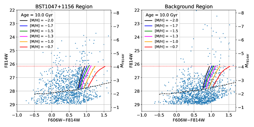
Figure 6: CMDs for BST1047 (left) and background (right) regions, overlaid with PARSEC 1.2S isochrones for 10 Gyr old populations of varying metallicities. These isochrones have been adjusted to reflect the small systematic photometric shifts in magnitude and color in our data as determined from the artificial star tests (see Section 2.2), but in the red these shifts are negligible at magnitudes brighter than F814W $\approx$ 27.5.

We compare the CMD of BST1047 to younger isochrones in Figure 8, which overplots the PARSEC 1.2S isochrones for a range of young and intermediate ages, using metallicities of [M/H] = $-2.0$, $-1.3$, and $-0.7$. We again adjust the isochrones for the systematic photometric shifts. At bright magnitudes (F814W$<$27) the shifts remain negligible, but in the blue at fainter magnitudes (F606W$-$F814W$<$0, F814W$>$27, the systematic blueward shift becomes more noticeable, shifting the isochrones bluer by $\approx 0.05-0.1$ mag near the 50% completeness limit and leading to the slight “bluish bulge” of the tracks in this region. With these effects in mind, these tracks show that the most luminous stars, 1–2 magnitudes brighter than the RGB tip, are consistent with blue and red helium burning sequences arising from massive stars younger than a few hundred million years old. At fainter magnitudes, the population of objects with very blue F606W$-$F814W colors $<0.0$ may be tracing massive main sequence stars as young as 50 Myr. Looking at the intermediate age RGB tracks, even at younger ages, RGB sequences are still generally too red to match the red sequence we see in BST1047, except perhaps at the very lowest metallicity ([M/H]$=-2$) and with relatively young ($<$2.5 Gyr) RGB populations. However, given the clear detection of BHeB stars in the same region, the most natural explanation for the red sequence in BST 1047 is that it is the associated RHeB sequence, with little evidence for a significant population of old RGB stars in the field.

In terms of metallicity, the sparseness of the stellar populations and the tight spacing of tracks within the helium burning sequences make it hard to give tight metallicity constraints for the population. Nonetheless, the stars are clearly metal poor, with [M/H] $\approx-1.0$ or somewhat lower. More metal-rich than this, the red helium burning sequences turn much redder than observed in BST1047 where the sequence remains bluer than F606W$-$F814W = 1.0. At the most metal-poor extreme, [M/H]=$-2.0$, both the red and blue helium burning tracks start to shift bluer than seen in the observed CMDs, making it unlikely that the populations are this metal-poor.

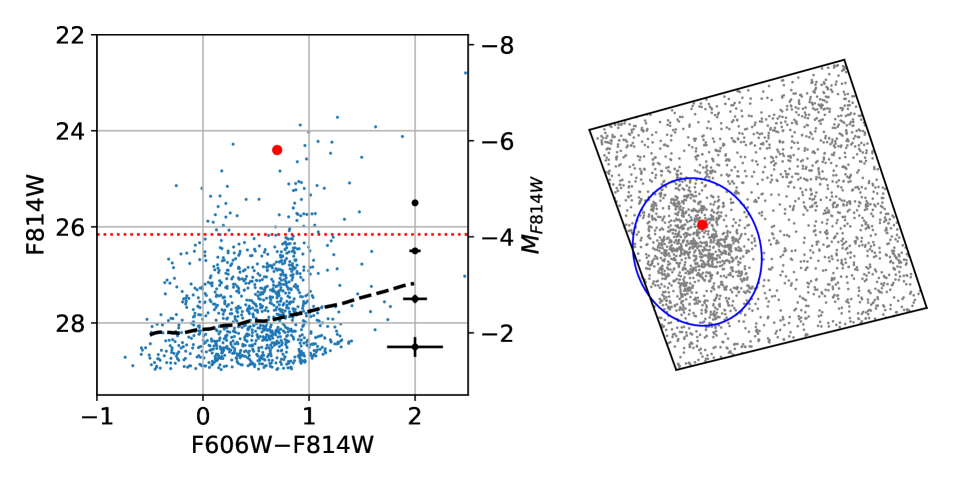
Figure 7: The CMD location (top) and spatial position (bottom) of the bright variable star detected in our imaging. In both plots, the red symbol shows the location of the variable. The CMD shows all point sources within the BST1047 region, which is shown by the blue oval in the lower panel. Lines and symbols in the CMD are as described in Figure 4, and the lower figure shows the 202″$\times$202″ACS field of view, with North up and East to the left.

In our photometry, we also find one variable star with properties potentially consistent with being a luminous Cepheid variable. The source is located 20″ north of the center of BST1047, at $(\alpha,\delta)_{J2000}$ = (10:47:43.32, +11:56:08.4). It has a mean magnitude of roughly F814W $\approx$ 24.4 and shows variability at the level of 0.35 mag in the individual ACS images, significantly larger than the single-image relative magnitude uncertainty of 0.05 mag at that magnitude. Because of the sparse cadence of our observations, secure photometry is difficult, but calculated from our two most concurrent F606W and F814W images (separated by 4.5 days), the object has a color of roughly F606W$-$F814=0.7, which would put it near the Cepheid instability strip in the F606W/F814W color-magnitude diagram (see, e.g.,  McCommas et al., 2009). While our data lack the proper cadence for accurate phasing, if the object is a Cepheid in BST1047, then with an absolute magnitude of $M_{\rm F814}=-5.8$ and using the F814W period-luminosity of Riess et al. (2019), the object would have a period of 26 days, roughly twice the time span of our imaging data, and consistent with the time variability we see in the source. Without proper imaging cadence, it is difficult to place strong constraints on the properties of the object, but if it is a Cepheid, that would also be consistent with the other signatures of young massive stars that we observe in BST1047.

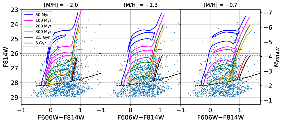
Figure 8: CMDs for BST1047 overlaid with PARSEC isochrones of stellar populations with varying ages and metallicities of [M/H]=$-2.0$ (left), $-1.3$ (middle), and $-0.7$ (right). These isochrones have been adjusted to reflect the small systematic photometric shifts in magnitude and color in our data as determined from the artificial star tests (see Section 2.2). These shifts in the isochrones are most noticeable as a slight blue “bulge” in the tracks at F814$>27.5$ and F606W$-$F814W $<0$.

So far in our analysis we have selected sources spatially, by region (sources within BST1047 vs those in the surrounding background region) and considered the CMDs of the regions separately. A complementary approach is to create a CMD for the entire ACS field, sub-select sources by their location within this full-field CMD, and ask where these subsamples are located spatially in the field. We show such an analysis in Figure 9. The panel at the top of the figure shows the CMD for the whole ACS image, where we have defined regions in the CMD that highlight the different putative stellar populations discussed so far. In particular, we highlight the blue and red helium burning sequences (‘BHeB’ and ‘RHeB’, respectively), the blue main sequence region (‘MS’), and the location of the older red giant branch population (‘RGB’). Selecting stars that fall in these regions in the CMD, we then plot in the bottom panels the spatial location of these CMD-selected sources.

Figure 9 clearly demonstrates that sources selected from CMD regions corresponding to young populations — the MS, BHeB, and RHeB regions — are preferentially found within BST1047. In contrast, objects drawn from the older RGB region are spread much more evenly across the ACS field, with no preferential clustering in or near BST1047. These spatial population patterns are consistent with a scenario in which BST1047 is dominated by recent star formation, with little or no evidence for an older stellar population. The smoothly distributed old RGB stars in the field are much more likely to come from M96’s stellar halo, with perhaps some additional contribution from Leo I intragroup stars (although any such contribution is likely to be small; Watkins et al., 2014; Ragusa et al., 2022). Additionally, there is a hint of a weak gradient in the spatial distribution of RGB stars across the ACS field. Comparing RGB counts on the western and eastern halves of the image, we find 54 RGB stars on the west side and 36 on the eastern side, roughly a $2\sigma$ difference. With M96 located 15′ southwest of the field, this gradient could be tracing the radial dropoff in M96’s halo population, or just a signature of patchiness in M96’s halo and/or the intragroup starlight in the region. For now we leave additional analysis and a more detailed discussion of the properties of the M96 halo population to a future paper.

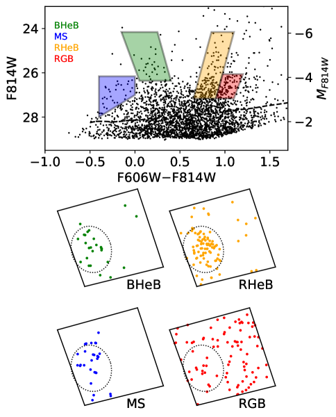
Figure 9: Spatial distribution of point sources in our ACS field, selected by their position on the color-magnitude diagram. The top panel shows the CMD for the full ACS field, with regions color coded by their presumed evolutionary stages. The bottom panels show the ACS field of view, mapping the point sources corresponding to each selected CMD region. Field orientation and scale is the same as in Figure 2, and the dotted oval shows the region containing BST1047.

4 The Origin of BST1047+1156

The detection of massive young stars in the blue and red helium burning sequences confirms a recent burst of star formation in BST1047, as originally inferred from the very blue broad-band colors of the galaxy’s integrated light (Mihos et al., 2018). The most luminous stars in these sequences have absolute magnitudes of $M_{\rm F814W}\approx-5$, consistent with massive stars ($M_{*}\approx 6-7$ $M_{\odot}$) with lifetimes $<$ 100 Myr, but the sequences continue down to fainter magnitudes ($M_{\rm F814W}\approx-3$) arguing for an extended phase of star formation extending to at least 300 Myr ago. However, this burst must have been relatively short lived; the lack of detected H$\alpha$ emission in BST1047 (Donahue et al., 1995) sets an upper limit on the present-day star formation rate of $\lesssim 5\times 10^{-5}$ $M_{\odot}$yr^-1 (Mihos et al., 2018). While we defer a full population modeling analysis to a future paper, we note here that not only are the red and blue population sequences consistent with a recent short burst of moderately metal-poor star formation, such a scenario is also quantitatively consistent with both the star counts seen in the HST imaging and the integrated light properties reported in Mihos et al. (2018). For example, using the PARSEC stellar population modeling tools (Bressan et al., 2012; Marigo et al., 2017, available at http://stev.oapd.inaf.it/cmd), a short (50 Myr) Gaussian burst of star formation of age $\sim 150$ Myr, mass $M_{*}=2\times 10^{10}$ $M_{\odot}$, [M/H]=-1.5 and a Kroupa (2001) initial mass function yields $\approx$ 40 bright stars in the range $-5\leq M_{F814W}\leq-4$ and $\approx$ 180 stars in the fainter range $-4\leq M_{F814W}\leq-3$. Performing a similar census of stars in the observed CMD and correcting for background as shown in 4 yields 40 $\pm$ 7 stars and 160 $\pm 15$ stars in the brighter and fainter magnitude range, respectively. This model also yields a total integrated B magnitude of $M_{B}=-10.1$ and color of $B-V=0.08$, compared to the measured values of $M_{B}=-10.2\pm 0.14$ and $B-V=0.14\pm 0.09$ (Mihos et al., 2018). Thus, all extant data are consistent with a recent, fading post starburst population in BST1047 that formed within the past few hundred million years.

Aside from the presence of high mass stars in BST1047, the other notable feature of its CMD is the lack of any prominent red giant branch population. While we cannot rule out a modest number of intermediate age ($<$ 5 Gyr) RGB stars, they would need to be very metal poor, with metallicities [M/H]$\sim-2$, to be hidden within the younger RHeB sequence. This lack of an old stellar population in BST1047 is in marked contrast to stellar populations of other types of diffuse star forming galaxies. The population of dwarf irregulars in the Local Group, while showing a wide variation of star formation histories, typically show old populations indicative of extended star formation histories (e.g.,  Grebel, 1997; Weisz et al., 2014), including even the extremely faint and diffuse dwarfs such as Leo T (Weisz et al., 2012) or Leo P (McQuinn et al., 2015). Another natural comparison would be to the population of blue, star-forming field low surface brightness galaxies. Resolved stellar population work in field LSBs has identified the helium burning sequences from evolving young stars (e.g.,  Schombert & McGaugh, 2014, 2015) as well as red giant branch stars that trace the older stellar populations (Schombert & McGaugh, 2021). The lack of RGB stars in BST1047 thus stands in contrast to the resolved populations in field LSBs, and more generally the integrated colors of field LSB galaxies are typically much redder than those of BST1047. For example, the $B-V$ color of BST1047 is 0.14 $\pm$ 0.09 (Mihos et al., 2018), compared to colors of $B-V\approx$ 0.3 – 0.6 for field LSBs (McGaugh & Bothun, 1994). Recent studies show that reddening from dust in LSBs is typically quite low (Junais et al., 2023), arguing that the redder colors of these field LSB galaxies indicate a substantial contribution of light from old stars relative to what we observe with BST1047. The lack of old stars in BST1047 likely then rules out scenarios where the galaxy is simply a extremely low surface brightness outlier in the population of star-forming field LSB galaxies.

The metallicities of the young stellar populations in BST1047 also argue against a model in which the object is a pre-existing low mass dwarf galaxy. Given the low inferred stellar mass for BST1047 (2–4 $\times 10^{5}$$M_{\odot}$, this work and Mihos et al. 2018), placing it on the mass-metallicity relationship for dwarf galaxies (e.g.,  Kirby et al., 2013) would predict a metallicity of [Fe/H]$=-2$, appreciably lower than the metallicity inferred from the analysis shown in Figure 8.

A more likely scenario for BST1047 is that it formed during a tidal interaction between galaxies within the Leo I Group. Tidal interactions can strip gas from the gas-rich outer disks of spiral galaxies, expelling that gas into the surrounding environment. Concurrently with the stripping the gas in the tidal debris can be collisionally compressed, leading to a burst of star formation and, potentially, to the formation of a tidal dwarf galaxy (e.g.,  Duc et al., 2000; Bournaud & Duc, 2006; Lelli et al., 2015). In this aspect, BST1047 may be most similar to (albeit fainter and much more diffuse than) tidal dwarf candidates found in the M81 group (Durrell et al., 2004; Mouhcine & Ibata, 2009; Chiboucas et al., 2013), which also appear to lack old stellar populations. Because tidal dwarfs form from pre-enriched material stripped from a larger host galaxy, these objects should also be elevated in metallicity compared to regular dwarf galaxies of the same mass (Duc & Mirabel, 1998; Weilbacher et al., 2003), just as we find for BST1047. Indeed, the metallicity of the young stars in BST1047 is comparable to that found in the outskirts of large spirals (e.g.,  Zaritsky et al., 1994; van Zee et al., 1998; Berg et al., 2020), and is also distinct from the higher, solar-like metallicities found in the Leo Ring to the north (Corbelli et al., 2021). Thus, the most likely origin for BST1047 is from gas that was stripped from the outer disk of the spiral galaxy M96, as also suggested by the distorted tidal HI morphology of M96’s outer disk (Figure 1 and Oosterloo et al., 2010).

Such a scenario would also explain the presence of massive young stars forming in an object with such low gas density, well below that more typically found in star forming environments (e.g.,  Bigiel et al., 2008, 2010; Wyder et al., 2009). If BST1047 formed during a tidal encounter, the initial compression of gas in the tidal caustics would have led to much higher gas densities capable of driving a weak starburst now traced by the young populations in BST1047. Subsequent tidal or ram-pressure stripping of the object, coupled perhaps with energy input from stellar winds and supernovae from the evolving starburst population, could have then dissociated the molecular gas and left BST1047 with a very diffuse ISM. The peak column density in BST1047 today is very low ($\sim$ 1 $M_{\odot}$ pc^-2 Mihos et al., 2018), and likely incapable of fueling any additional star formation. While the relatively large beam size of the HI data leaves open the possibility of pockets of high density gas on small scales, recent CO observations of BST1047 have failed to detect molecular gas in the system (Corbelli et al., 2023), although those studies did not survey BST1047’s full HI extent. Nonetheless, there is no evidence for any current, ongoing star formation in BST1047 today.

The ultimate fate of BST1047 remains unclear. Its HI morphology (Figure 1) shows streamers of HI extending to the southeast towards M96, likely a signature of tidal stripping of BST1047, or perhaps ram-pressure stripping from hot gas in M96’s halo or the group environment. BST1047’s very low density makes it susceptible to stripping processes, particularly if it is a tidal dwarf with no cocooning halo of dark matter to keep it bound. Mihos et al. (2018) used the observed HI kinematics to show that BST1047’s dynamical mass and baryonic mass were comparable ($\sim 5-6\times 10^{7}$ $M_{\odot}$), providing support for the idea that the object lacks dark matter, as expected for tidal dwarfs. If BST1047 is in the process of being disrupted by the environment of the Leo I Group, we may be catching this object in a very transitory phase, with its fading post-starburst population soon to be stripped and expelled into the group environment. As such, the galaxy may be a prime example of a “failing” tidal dwarf, born in the tidal debris of a recent encounter, but lacking sufficient mass to overcome the destructive dynamical processes found within the group environment.

5 Summary

We have used deep Hubble ACS imaging in F606W/F814W to study the resolved stellar populations in the gas-rich ultradiffuse object BST1047+1156 in the Leo I Group. At zero color, our photometry reaches limiting magnitudes of F606W_lim=28.7 and F814W_lim=28.2, extending two magnitudes down the red giant branch at the 11.0 Mpc distance of the Leo I Group. We clearly detect the stellar population associated with BST1047, identifying the red and blue helium burning sequences expected from an evolving population of massive stars. We also find an excess of fainter blue stars likely to be slightly less massive stars still on the main sequence. The distribution of color and luminosity of stars in BST1047 are consistent with a modestly metal poor stellar population ([M/H] $\sim-1.0$ to $-1.5$) with ages of a few hundred million years, consistent with the integrated colors and surface brightness measured in ground based imaging (Mihos et al., 2018).

However, we find no trace of a red giant branch sequence in the stellar populations of BST1047 despite going sufficiently deep to detect such stars. This lack of an old stellar population argues strongly against scenarios in which BST1047 is a long lived LSB galaxy that has merely had a weak burst of star formation due to interactions within the group environment. Instead, the combination of its exclusively young and moderately metal-poor stellar populations, its diffuse nature, and its disturbed HI morphology argues that we are seeing a transient object, likely formed from gas recently stripped from the outer disk of M96 due to tidal forces at work within the group environment. These tidal forces continue to strip gas and stars away from BST1047 today, feeding the the intragroup stellar population of the Leo I Group. BST1047 is thus likely to be a failing tidal dwarf, formed from the tidal debris of M96 but with such low density that it is destined to ultimately disperse into the intragroup population of the Leo I group.

Finally, in the environment surrounding BST1047, we also clearly detect red giant stars in the stellar halo of M96. These stars are distributed fairly uniformly across the ACS field of view, showing no spatial correlation with the location of BST1047. From the location of the red giant sequence on the color-magnitude diagram we infer a moderately low stellar metallicity of [M/H] $\approx-1.3\pm 0.2$. These data probe the stellar populations in the galaxy’s outer halo at the extremely large projected radial distance of 50 kpc, and we plan a future paper incorporating the data from the adjacent WFC3 parallel field to study the properties of M96’s outer stellar halo in more detail.

References

- The Astropy Collaboration (2013) Astropy Collaboration, Robitaille, T. P., Tollerud, E. J., et al. 2013, A&A, 558, A33. doi:10.1051/0004-6361/201322068
- The Astropy Collaboration (2018) The Astropy Collaboration 2018, AJ, 156, 123. doi:10.3847/1538-3881/aabc4f
- The Astropy Collaboration (2022) Astropy Collaboration, Price-Whelan, A. M., Lim, P. L., et al. 2022, ApJ, 935, 167. doi:10.3847/1538-4357/ac7c74
- Barnes & Hernquist (1992) Barnes, J. E. & Hernquist, L. 1992, Nature, 360, 715. doi:10.1038/360715a0
- Bertin & Arnouts (1996) Bertin, E. & Arnouts, S. 1996, A&AS, 117, 393.
- Berg et al. (2020) Berg, D. A., Pogge, R. W., Skillman, E. D., et al. 2020, ApJ, 893, 96. doi:10.3847/1538-4357/ab7eab
- Bigiel et al. (2010) Bigiel, F., Leroy, A., Walter, F., et al. 2010, AJ, 140, 1194. doi:10.1088/0004-6256/140/5/1194
- Bigiel et al. (2008) Bigiel, F., Leroy, A., Walter, F., et al. 2008, AJ, 136, 2846. doi:10.1088/0004-6256/136/6/2846
- Bournaud & Duc (2006) Bournaud, F. & Duc, P.-A. 2006, A&A, 456, 481. doi:10.1051/0004-6361:20065248
- Bressan et al. (2012) Bressan, A., Marigo, P., Girardi, L., et al. 2012, MNRAS, 427, 127. doi:10.1111/j.1365-2966.2012.21948.x
- Cannon et al. (2015) Cannon, J. M., Martinkus, C. P., Leisman, L., et al. 2015, AJ, 149, 72. doi:10.1088/0004-6256/149/2/72
- Chiboucas et al. (2013) Chiboucas, K., Jacobs, B. A., Tully, R. B., et al. 2013, AJ, 146, 126. doi:10.1088/0004-6256/146/5/126
- Clark & Glover (2014) Clark, P. C. & Glover, S. C. O. 2014, MNRAS, 444, 2396. doi:10.1093/mnras/stu1589
- Corbelli et al. (2021) Corbelli, E., Cresci, G., Mannucci, F., et al. 2021, ApJ, 908, L39. doi:10.3847/2041-8213/abdf64
- Corbelli et al. (2023) Corbelli, E., Thilker, D., Mannucci, F., et al. 2023, A&A, 671, A104. doi:10.1051/0004-6361/202244941
- Dolphin (2000) Dolphin, A. E. 2000, PASP, 112, 1383. doi:10.1086/316630
- Donahue et al. (1995) Donahue, M., Aldering, G., & Stocke, J. T. 1995, ApJ, 450, L45. doi:10.1086/316771
- Duc et al. (2000) Duc, P.-A., Brinks, E., Springel, V., et al. 2000, AJ, 120, 1238. doi:10.1086/301516
- Duc & Mirabel (1998) Duc, P.-A. & Mirabel, I. F. 1998, A&A, 333, 813
- Durrell et al. (2004) Durrell, P. R., Decesar, M. E., Ciardullo, R., et al. 2004, Recycling Intergalactic and Interstellar Matter, 217, 90. doi:10.48550/arXiv.astro-ph/0311130
- Ellison et al. (2008) Ellison, S. L., Patton, D. R., Simard, L., et al. 2008, ApJ, 672, L107. doi:10.1086/527296
- Elmegreen et al. (1993) Elmegreen, B. G., Kaufman, M., & Thomasson, M. 1993, ApJ, 412, 90. doi:10.1086/172903
- Girardi et al. (2005) Girardi, L., Groenewegen, M. A. T., Hatziminaoglou, E., et al. 2005, A&A, 436, 895. doi:10.1051/0004-6361:20042352
- Girardi (2016) Girardi, L. 2016, Astronomische Nachrichten, 337, 871. doi:10.1002/asna.201612388
- Graham et al. (1997) Graham, J. A., Phelps, R. L., Freedman, W. L., et al. 1997, ApJ, 477, 535. doi:10.1086/303740
- Grebel (1997) Grebel, E. K. 1997, Reviews in Modern Astronomy, 10, 29
- Harmsen et al. (2017) Harmsen, B., Monachesi, A., Bell, E. F., et al. 2017, MNRAS, 466, 1491. doi:10.1093/mnras/stw2992
- Harris et al. (2020) Harris, C.R., Millman, K.J., van der Walt, S.J. et al. 2020, Nature, 585, 357
- Hunter et al. (2007) Hunter, J.D., 2007, Computing in Science and Engineering, 9:3, 90.
- Jang & Lee (2017) Jang, I. S. & Lee, M. G. 2017, ApJ, 836, 74. doi:10.3847/1538-4357/836/1/74
- Junais et al. (2023) Junais, Małek, K., Boissier, S., et al. 2023, A&A, 676, A41. doi:10.1051/0004-6361/202346528
- Kirby et al. (2013) Kirby, E. N., Cohen, J. G., Guhathakurta, P., et al. 2013, ApJ, 779, 102. doi:10.1088/0004-637X/779/2/102
- Krist (1995) Krist, J. 1995, Astronomical Data Analysis Software and Systems IV, 77, 349
- Kroupa (2001) Kroupa, P. 2001, MNRAS, 322, 231. doi:10.1046/j.1365-8711.2001.04022.x
- Krumholz et al. (2009) Krumholz, M. R., McKee, C. F., & Tumlinson, J. 2009, ApJ, 699, 850. doi:10.1088/0004-637X/699/1/850
- Lee et al. (2006) Lee, H., Skillman, E. D., Cannon, J. M., et al. 2006, ApJ, 647, 970. doi:10.1086/505573
- Lee & Jang (2016) Lee, M. G. & Jang, I. S. 2016, ApJ, 822, 70. doi:10.3847/0004-637X/822/2/70
- Lee et al. (2017) Lee, M. G., Kang, J., Lee, J. H., et al. 2017, ApJ, 844, 157. doi:10.3847/1538-4357/aa78fb
- Leisman et al. (2017) Leisman, L., Haynes, M. P., Janowiecki, S., et al. 2017, ApJ, 842, 133. doi:10.3847/1538-4357/aa7575
- Lelli et al. (2015) Lelli, F., Duc, P.-A., Brinks, E., et al. 2015, A&A, 584, A113. doi:10.1051/0004-6361/201526613
- Lotz et al. (2017) Lotz, J. M., Koekemoer, A., Coe, D., et al. 2017, ApJ, 837, 97. doi:10.3847/1538-4357/837/1/97
- Marigo et al. (2017) Marigo, P., Girardi, L., Bressan, A., et al. 2017, ApJ, 835, 77. doi:10.3847/1538-4357/835/1/77
- McCommas et al. (2009) McCommas, L. P., Yoachim, P., Williams, B. F., et al. 2009, AJ, 137, 4707. doi:10.1088/0004-6256/137/6/4707
- McGaugh & Bothun (1994) McGaugh, S. S. & Bothun, G. D. 1994, AJ, 107, 530. doi:10.1086/116874
- McQuinn et al. (2015) McQuinn, K. B. W., Skillman, E. D., Dolphin, A., et al. 2015, ApJ, 812, 158. doi:10.1088/0004-637X/812/2/158
- Michel-Dansac et al. (2010) Michel-Dansac, L., Duc, P.-A., Bournaud, F., et al. 2010, ApJ, 717, L143. doi:10.1088/2041-8205/717/2/L143
- Mihos et al. (2018) Mihos, J. C., Carr, C. T., Watkins, A. E., et al. 2018, ApJ, 863, L7. doi:10.3847/2041-8213/aad62e
- Mihos et al. (2018) Mihos, J. C., Durrell, P. R., Feldmeier, J. J., et al. 2018, ApJ, 862, 99. doi:10.3847/1538-4357/aacd14
- Mihos et al. (2022) Mihos, J. C., Durrell, P. R., Toloba, E., et al. 2022, ApJ, 924, 87. doi:10.3847/1538-4357/ac35d9
- Monachesi et al. (2016) Monachesi, A., Bell, E. F., Radburn-Smith, D. J., et al. 2016, MNRAS, 457, 1419. doi:10.1093/mnras/stv2987
- Mouhcine & Ibata (2009) Mouhcine, M. & Ibata, R. 2009, MNRAS, 399, 737. doi:10.1111/j.1365-2966.2009.15135.x
- Oosterloo et al. (2010) Oosterloo, T., Morganti, R., Crocker, A., et al. 2010, MNRAS, 409, 500. doi:10.1111/j.1365-2966.2010.17351.x
- Pilyugin et al. (2014) Pilyugin, L. S., Grebel, E. K., Zinchenko, I. A., et al. 2014, AJ, 148, 134. doi:10.1088/0004-6256/148/6/134
- Ragusa et al. (2022) Ragusa, R., Mirabile, M., Spavone, M., et al. 2022, Frontiers in Astronomy and Space Sciences, 9, 852810. doi:10.3389/fspas.2022.852810
- Riess et al. (2019) Riess, A. G., Casertano, S., Yuan, W., et al. 2019, ApJ, 876, 85. doi:10.3847/1538-4357/ab1422
- Salaris et al. (1993) Salaris, M., Chieffi, A., & Straniero, O. 1993, ApJ, 414, 580. doi:10.1086/173105
- Schlafly & Finkbeiner (2011) Schlafly, E. F. & Finkbeiner, D. P. 2011, ApJ, 737, 103. doi:10.1088/0004-637X/737/2/103
- Schneider (1985) Schneider, S. 1985, ApJ, 288, L33. doi:10.1086/184416
- Schneider et al. (1986) Schneider, S. E., Salpeter, E. E., & Terzian, Y. 1986, AJ, 91, 13. doi:10.1086/113975
- Schombert & McGaugh (2014) Schombert, J. & McGaugh, S. 2014, PASA, 31, e036. doi:10.1017/pasa.2014.32
- Schombert & McGaugh (2015) Schombert, J. & McGaugh, S. 2015, AJ, 150, 72. doi:10.1088/0004-6256/150/3/72
- Schombert & McGaugh (2021) Schombert, J. & McGaugh, S. 2021, AJ, 161, 91. doi:10.3847/1538-3881/abd54d
- Schombert et al. (2001) Schombert, J. M., McGaugh, S. S., & Eder, J. A. 2001, AJ, 121, 2420. doi:10.1086/320398
- Shen et al. (2021) Shen, Z., van Dokkum, P., & Danieli, S. 2021, ApJ, 909, 179. doi:10.3847/1538-4357/abdd29
- Streich et al. (2014) Streich, D., de Jong, R. S., Bailin, J., et al. 2014, A&A, 563, A5. doi:10.1051/0004-6361/201220956
- van der Hulst et al. (1993) van der Hulst, J. M., Skillman, E. D., Smith, T. R., et al. 1993, AJ, 106, 548. doi:10.1086/116660
- van Zee et al. (1997) van Zee, L., Haynes, M. P., Salzer, J. J., et al. 1997, AJ, 113, 1618. doi:10.1086/118379
- van Zee et al. (1998) van Zee, L., Salzer, J. J., Haynes, M. P., et al. 1998, AJ, 116, 2805. doi:10.1086/300647
- Virtanen et al. (2020) Virtanen, P., Gommers, R., Oliphant, T. E. et al. 2020, Nature Methods, 17, 261
- Watkins et al. (2014) Watkins, A. E., Mihos, J. C., Harding, P., et al. 2014, ApJ, 791, 38. doi:10.1088/0004-637X/791/1/38
- Weilbacher et al. (2003) Weilbacher, P. M., Duc, P.-A., & Fritze-v. Alvensleben, U. 2003, A&A, 397, 545. doi:10.1051/0004-6361:20021522
- Weisz et al. (2012) Weisz, D. R., Zucker, D. B., Dolphin, A. E., et al. 2012, ApJ, 748, 88. doi:10.1088/0004-637X/748/2/88
- Weisz et al. (2014) Weisz, D. R., Dolphin, A. E., Skillman, E. D., et al. 2014, ApJ, 789, 147. doi:10.1088/0004-637X/789/2/147
- Williams et al. (2014) Williams, B. F., Lang, D., Dalcanton, J. J., et al. 2014, ApJS, 215, 9. doi:10.1088/0067-0049/215/1/9
- Wyder et al. (2009) Wyder, T. K., Martin, D. C., Barlow, T. A., et al. 2009, ApJ, 696, 1834. doi:10.1088/0004-637X/696/2/1834
- Zaritsky et al. (1994) Zaritsky, D., Kennicutt, R. C., & Huchra, J. P. 1994, ApJ, 420, 87. doi:10.1086/173544