On the infinite time horizon approximation for Lévy-driven McKean-Vlasov SDEs with non-globally Lipschitz continuous and super-linearly growth drift and diffusion coefficients

Abstract

This paper studies the numerical approximation for McKean-Vlasov stochastic differential equations driven by Lévy processes. We propose a tamed-adaptive Euler-Maruyama scheme and consider its strong convergence in both finite and infinite time horizons when applying for some classes of Lévy-driven McKean-Vlasov stochastic differential equations with non-globally Lipschitz continuous and super-linearly growth drift and diffusion coefficients.

Keywords Lévy process $\cdot$ McKean-Vlasov $\cdot$ Stochastic differential equation $\cdot$ Super-linearly growth coefficient $\cdot$ Tamed-adaptive Euler Maruyama

Mathematics Subject Classification: 60H35, 60H10

1 Introduction

On a complete probability space $(\Omega,\mathcal{F},\mathbb{P})$, we consider the $d$-dimensional process $X=(X_{t})_{t\geq 0}$ solution to the following McKean-Vlasov stochastic differential equation (SDE) with jumps

$$dX_{t}=b(X_{t},\mathcal{L}_{X_{t}})dt+\sigma(X_{t},\mathcal{L}_{X_{t}})dW_{t}+c\left(X_{t-},\mathcal{L}_{X_{t-}}\right)dZ_{t},$$ (1)

for $t\geq 0$, where $X_{0}=x_{0}\in\mathbb{R}^{d}$ is a fixed initial value, $\mathcal{L}_{X_{t}}$ denotes the marginal law of the process $X$ at time $t$, $W=(W_{t})_{t\geq 0}$ is a $d$-dimensional standard Brownian motion and $Z=(Z_{t})_{t\geq 0}$ is a $d$-dimensional centered pure jump Lévy process whose Lévy measure $\nu$ satisfies $\int_{\mathbb{R}^{d}}(1\wedge|z|^{2})\nu(dz)<+\infty$. Two processes $W$ and $Z$ are supposed to be independent. The natural filtration $(\mathcal{F}_{t})_{t\geq 0}$ is generated by $W$ and $Z$. The Lévy-Itô decomposition of $Z$ is given by

$$Z_{t}=\int_{0}^{t}\int_{\mathbb{R}_{0}^{d}}z(N(ds,dz)-\nu(dz)ds),$$

for any $t\geq 0$, where $\mathbb{R}_{0}^{d}:=\mathbb{R}^{d}\setminus\{0\}$, and $N(dt,dz)$ is a Poisson random measure on the measurable space $(\mathbb{R}_{+}\times\mathbb{R}_{0}^{d},\mathcal{B}(\mathbb{R}_{+}\times\mathbb{R}_{0}^{d}))$ that is associated with the jumps of the Lévy process $Z$ with intensity measure $\nu(dz)dt$. That is,

$$N(dt,dz):=\sum_{0\leq s\leq t}{\bf 1}_{\{\Delta Z_{s}\neq 0\}}\delta_{(s,\Delta Z_{s})}(ds,dz).$$

Here, the jump size of $Z$ at instant $s$ is defined as $\Delta Z_{s}:=Z_{s}-Z_{s-}:=Z_{s}-\lim_{u\uparrow s}Z_{u}$ for any $s>0$, $\Delta Z_{0}:=0$, $\delta_{(s,z)}$ denotes the Dirac measure at the point $(s,z)\in\mathbb{R}_{+}\times\mathbb{R}_{0}^{d}$, and $\mathcal{B}(\mathbb{R}_{+}\times\mathbb{R}_{0}^{d})$ denotes the Borel $\sigma$-algebra on $\mathbb{R}_{+}\times\mathbb{R}_{0}^{d}$. The compensated Poisson random measure associated with $N(dt,dz)$ is denoted by $\widetilde{N}(dt,dz):=N(dt,dz)-\nu(dz)dt$.

We denote by $\mathcal{P}(\mathbb{R}^{d})$ the space of all probability measures defined on a measurable space $(\mathbb{R}^{d},\mathcal{B}(\mathbb{R}^{d}))$, where $\mathcal{B}(\mathbb{R}^{d})$ denotes the Borel $\sigma$-field over $\mathbb{R}^{d}$, and by

$$\mathcal{P}_{2}(\mathbb{R}^{d}):=\left\{\mu\in\mathcal{P}(\mathbb{R}^{d}):\int_{\mathbb{R}^{d}}|x|^{2}\mu(dx)<\infty\right\}$$

the subset of probability measures with the finite second moment. As metric on the space $\mathcal{P}_{2}(\mathbb{R}^{d})$, we use the $\mathcal{L}_{2}$-Wasserstein distance. That is, for $\mu,\nu\in\mathcal{P}_{2}(\mathbb{R}^{d})$, the $\mathcal{L}_{2}$-Wasserstein distance between $\mu$ and $\nu$ is defined as

$$\mathcal{W}_{2}(\mu,\nu):=\inf_{\pi\in\mathcal{C}(\mu,\nu)}\left(\int_{\mathbb{R}^{d}\times\mathbb{R}^{d}}\left|x-y\right|^{2}\pi(dx,dy)\right)^{1/2},$$

where $\mathcal{C}(\mu,\nu)$ denotes all the couplings of $\mu$ and $\nu$. That is, $\pi\in\mathcal{C}(\mu,\nu)$ if and only if $\pi(\cdot,\mathbb{R}^{d})=\mu(\cdot)$ and $\pi(\mathbb{R}^{d},\cdot)=\nu(\cdot)$.

The coefficients $b=(b_{i})_{1\leq i\leq d}:\mathbb{R}^{d}\times\mathcal{P}_{2}(\mathbb{R}^{d})\to\mathbb{R}^{d}$, $\sigma=(\sigma_{ij})_{1\leq i,j\leq d}:\mathbb{R}^{d}\times\mathcal{P}_{2}(\mathbb{R}^{d})\to\mathbb{R}^{d}\otimes\mathbb{R}^{d}$ and $c=(c_{ij})_{1\leq i,j\leq d}:\mathbb{R}^{d}\times\mathcal{P}_{2}(\mathbb{R}^{d})\to\mathbb{R}^{d}\otimes\mathbb{R}^{d}$ are measurable functions. The integral equation (1) now writes as

$$X_{t}=x_{0}+\int_{0}^{t}b(X_{s},\mathcal{L}_{X_{s}})ds+\int_{0}^{t}\sigma(X_{s},\mathcal{L}_{X_{s}})dW_{s}+\int_{0}^{t}\int_{\mathbb{R}_{0}^{d}}c\left(X_{s-},\mathcal{L}_{X_{s-}}\right)z\widetilde{N}(ds,dz),$$

for any $t\geq 0$.

The McKean-Vlasov process was first studied by McKean in [26] as a model for the Vlasov equation describing the time evolution of the distribution function of a plasma consisting of charged particles with long-range interaction. The process can be obtained as a limit of a mean-field system of interacting particles as the number of particles tends to infinity. The very first studies on the numerical approximation for McKean-Vlasov SDEs are the works of Ogawa [28], Kohatsu-Higa and Ogawa [18] and Bossy and Talay [3], where the authors considered the weak approximation of McKean-Vlasov SDEs with regular coefficients. However, the numerical approximation for McKean-Vlasov SDEs has only become active in the last decade.

Let $X^{(n)}_{T}$ be an approximation of $X_{T}$ which depends on the values of $W$ and $Z$ at fixed equidistance times $t_{k}=\frac{kT}{n},k=0,1,\ldots,n$. Then under some regularity conditions on the coefficients $b,\sigma,$ and $c$, one may prove that

$$\|X^{(n)}_{T}-X_{T}\|_{L^{p}}:=\Big{(}\mathbb{E}[|X^{(n)}_{T}-X_{T}|^{p}]\Big{)}^{1/p}\leq\frac{C(T)}{n^{\zeta_{0}}},$$ (2)

for some positive constants $p$ and ${\zeta_{0}}$. In case the estimate (2) holds, we say that the $X^{(n)}_{T}$ converges at the rate of order ${\zeta_{0}}$ in $L^{p}$-norm.

It is now well-known that for SDEs with super-linear growth coefficients, the Euler-Maruyama scheme may not converge in the $L^{p}$-norm (see [13]). Therefore, the numerical approximation for SDEs with super-linear growth coefficients has attracted lots of attention recently. New approximation schemes have been introduced to solve the problem, such as the tamed Euler-Maruyama scheme ([14, 31, 32, 21]), the truncated Euler-Maruyama scheme ([24]), the implicit Euler-Maruyama scheme ([25]), the adaptive Euler-Maruyama scheme ([10]). In [7, 19, 20, 23] the tamed Euler-Maruyama scheme has been developed to approximate McKean-Vlasov SDEs with super-linear growth coefficients. In [29], the authors introduced several adaptive Euler-Maruyama and Milstein schemes and studied their strong rate of convergence for McKean-Vlasov SDEs with super-linear drift. In [15], the authors introduced a multilevel Picard approximation, which has a low computational cost, for McKean-Vlasov SDEs with additive noise. In [6, 7], the authors introduced the implicit Euler-Maruyama scheme and studied its convergence in $L^{p}$-norm for McKean-Vlasov SDEs with drifts of super-linear growth.

The McKean-Vlasov SDEs with jumps were studied by many authors with applications in many domains (see [12, 8, 9, 1, 11] and the reference therein). In [27], the authors considered McKean-Vlasov SDEs driven by infinite activity Lévy processes with super-linear growth coefficients. They proved the existence and uniqueness of the solution and proposed a tamed Euler-Maruyama approximation for the associated interacting particle system and proved that the rate of its convergence in $L^{p}$-norm is arbitrarily close to 0.5.

In some applications, it is necessary to approximate $X_{T}$ for $T$ large, e.g., to approximate the invariant distribution of process $X$ (see Section 3 in [10]). However, since the proof of convergence of many schemes often involves Gronwall’s inequality, the quantity $C(T)$ may grow exponentially fast to $T$. Recently, there have been some attempts to introduce numerical schemes where $C(T)$ does not depend on $T$. The paper [10] proposed an adaptive Euler-Maruyama scheme for SDEs where each stepsize is adjusted to the size of the current values of $X$, and showed its strong convergence in the interval $[0,\infty)$ when applying for SDEs whose coefficients $b$ and $\sigma$ satisfy the contractive Lipschitz condition (Assumption 9 in [10]), $b$ is polynomial growth Lipschitz continuous, and $\sigma$ is bounded and globally Lipschitz continuous. The paper [16] introduced a tamed-adaptive Euler-Maruyama scheme and considered its rate of convergence in $L^{1}$-norm when applying for one-dimensional SDEs whose diffusion coefficient $\sigma$ is of super-linearly growth. In [17], the result of [16] was generalized for one-dimensional SDEs with jumps.

This paper aims to generalize the result of the papers [10, 16, 17] for multi-dimensional McKean-Vlasov SDEs with jumps. In particular, we propose a tamed-adaptive Euler-Maruyama approximation scheme for the Lévy-driven SDEs (1) where $\sigma$ and $b$ are non-globally Lipschitz continuous and of super-linearly growth, and $c$ is Lipschitz continuous. We will study the strong convergence of the scheme in both finite and infinite time intervals. Note that in [29] the authors only considered the strong convergence of their adaptive scheme in a fixed time interval. In [27], the tamed Euler-Maruyama scheme is also proven to converge in a fixed time interval when applying for McKean-Vlasov SDEs with jumps. To the best of our knowledge, our tamed-adaptive Euler-Maruyama scheme is the first approximation method for Lévy driven McKean-Vlasov SDEs that could be shown to converge in an infinite time horizon.

We denote the vector Euclidean norm of $v$ by $|v|:=(|v_{1}|^{2}+|v_{2}|^{2}+\ldots+|v_{d}|^{2})^{\frac{1}{2}}$, the inner product of vectors $v$ and $w$ by $\langle v,w\rangle:=v_{1}w_{1}+v_{2}w_{2}+\ldots+v_{d}w_{d}$ for any $v,w\in\mathbb{R}^{d}$, the Frobenius matrix norm by $|A|:=\sqrt{\sum_{i,j=1}^{d}A^{2}_{ij}}$ for all $A\in\mathbb{R}^{d\times d}$, the integer part of $a$ by $[a]$, and the transpose of a vector or matrix $A$ by $A^{\mathsf{T}}$. Moreover, the binomial coefficients are denoted by ${n\choose k}:=\frac{n!}{k!(n-k)!}$. In all that follows, we denote by $C$ positive constants whose value may change from one line to the next.

The rest of this paper is structured as follows. In Section 2, we introduce assumptions on the coefficients of equation (1) and show some moment estimates under these assumptions. In Section 3, we prove the propagation of chaos. In Section 4, we introduce the tamed-adaptive Euler-Maruyama scheme and prove that it is well-defined and converges in $L^{2}$-norm. Section 5 presents a numerical study for the tamed-adaptive Euler-Maruyama scheme.

2 Model assumptions and moment estimates

Assume that the drift, diffusion and jump coefficients $b,\sigma,c$ and the Lévy measure $\nu$ of equation (1) satisfy the following conditions:

1. There exists a positive constant $L$ such that

   $$2\left\langle x,b(x,\mu)\right\rangle+\left|\sigma(x,\mu)\right|^{2}+|c(x,\mu)|^{2}\int_{\mathbb{R}_{0}^{d}}|z|^{2}\nu(dz)\leq L\left(1+|x|^{2}+\mathcal{W}_{2}^{2}(\mu,\delta_{0})\right),$$

   for any $x\in\mathbb{R}^{d}$ and $\mu\in\mathcal{P}_{2}(\mathbb{R}^{d})$.

2. There exist constants $\kappa_{1}>0,\kappa_{2}>0$, $L_{1}\in\mathbb{R}$ and $L_{2}\geq 0$ such that

   $$2\left\langle x-\overline{x},b(x,\mu)-b(\overline{x},\overline{\mu})\right\rangle+\kappa_{1}\left|\sigma(x,\mu)-\sigma(\overline{x},\overline{\mu})\right|^{2}+\kappa_{2}|c(x,\mu)-c(\overline{x},\overline{\mu})|^{2}\int_{\mathbb{R}_{0}^{d}}|z|^{2}\nu(dz)$$

   $$\leq L_{1}|x-\overline{x}|^{2}+L_{2}\mathcal{W}_{2}^{2}(\mu,\overline{\mu}),$$

   for any $x,\overline{x}\in\mathbb{R}^{d}$ and $\mu,\overline{\mu}\in\mathcal{P}_{2}(\mathbb{R}^{d})$.

3. $b(x,\mu)$ is a continuous function of $x\in\mathbb{R}^{d}$ and $\mu\in\mathcal{P}_{2}(\mathbb{R}^{d})$.

4. There exist constants $L>0$ and $\ell\geq 0$ such that

   $$\left|b(x,\mu)-b(\overline{x},\overline{\mu})\right|\leq L\left(1+|x|^{\ell}+|\overline{x}|^{\ell}\right)\left(|x-\overline{x}|+\mathcal{W}_{2}(\mu,\overline{\mu})\right),$$

   for any $x,\overline{x}\in\mathbb{R}^{d}$ and $\mu,\overline{\mu}\in\mathcal{P}_{2}(\mathbb{R}^{d})$.

5. There exists an even integer $p_{0}\in[2,+\infty)$ such that $\int_{|z|>1}|z|^{p_{0}}\nu(dz)<\infty$ and $\int_{0<|z|\leq 1}|z|\nu(dz)<\infty$.

6. There exists a positive constant $L_{3}$ such that

   $$|c(x,\mu)|\leq L_{3}\left(1+|x|+\mathcal{W}_{2}(\mu,\delta_{0})\right),$$

   for any $\;x\in\mathbb{R}^{d}$ and $\mu\in\mathcal{P}_{2}(\mathbb{R}^{d})$.

7. For the even integer $p_{0}\in[2,+\infty)$ given in A5 and the positive constant $L_{3}$ given in A6, there exist constants $\gamma_{1}\in\mathbb{R}$, $\gamma_{2}\geq 0$ and $\eta\geq 0$ such that

   $$\langle x,b(x,\mu)\rangle+\dfrac{p_{0}-1}{2}|\sigma(x,\mu)|^{2}+\dfrac{1}{2L_{3}}|c(x,\mu)|^{2}\int_{\mathbb{R}_{0}^{d}}|z|\left(\left(1+L_{3}|z|\right)^{p_{0}-1}-1\right)\nu(dz)\leq\gamma_{1}|x|^{2}+\gamma_{2}\mathcal{W}_{2}^{2}(\mu,\delta_{0})+\eta,$$

   for any $x\in\mathbb{R}^{d}$ and $\mu\in\mathcal{P}_{2}(\mathbb{R}^{d})$.

Remark 2.1.

(i) It follows from Condition A4 that

$$\left|b(x,\mu)\right|\leq\left|b(0,\delta_{0})\right|+L\left(1+|x|^{\ell}\right)\left(|x|+\mathcal{W}_{2}(\mu,\delta_{0})\right),$$

for any $x\in\mathbb{R}^{d}$ and $\mu\in\mathcal{P}_{2}(\mathbb{R}^{d})$.

(ii) Assume that Condition A2 holds for $\kappa_{1}=\kappa_{2}=1+\varepsilon$, $L_{1}\in\mathbb{R}$, $L_{2}\geq 0$ with a constant $\varepsilon>0$ . This, combined with Condition A4 and Cauchy’s inequality, implies that

$$\left(1+\varepsilon\right)\left|\sigma(x,\mu)-\sigma(\overline{x},\overline{\mu})\right|^{2}+\left(1+\varepsilon\right)|c(x,\mu)-c(\overline{x},\overline{\mu})|^{2}\int_{\mathbb{R}_{0}^{d}}|z|^{2}\nu(dz)$$

$$\leq 2|x-\overline{x}||b(x,\mu)-b(\overline{x},\overline{\mu})|+L_{1}|x-\overline{x}|^{2}+L_{2}\mathcal{W}_{2}^{2}(\mu,\overline{\mu})$$

$$\leq L\left(1+|x|^{\ell}+|\overline{x}|^{\ell}\right)\left(2|x-\overline{x}|^{2}+2|x-\overline{x}|\mathcal{W}_{2}(\mu,\overline{\mu})\right)+L_{1}|x-\overline{x}|^{2}+L_{2}\mathcal{W}_{2}^{2}(\mu,\overline{\mu})$$

$$\leq L\left(1+|x|^{\ell}+|\overline{x}|^{\ell}\right)\left(2|x-\overline{x}|^{2}+|x-\overline{x}|^{2}+\mathcal{W}_{2}^{2}(\mu,\overline{\mu})\right)+L_{1}|x-\overline{x}|^{2}+L_{2}\mathcal{W}_{2}^{2}(\mu,\overline{\mu})$$

$$\leq L\widetilde{L}\left(1+|x|^{\ell}+|\overline{x}|^{\ell}\right)\left(|x-\overline{x}|^{2}+\mathcal{W}_{2}^{2}(\mu,\overline{\mu})\right),$$

with $\widetilde{L}=\max\{3,L_{1},L_{2}\}$ for any $x,\overline{x}\in\mathbb{R}^{d}$ and $\mu,\overline{\mu}\in\mathcal{P}_{2}(\mathbb{R}^{d})$. This yields to

$$\left|\sigma(x,\mu)-\sigma(\overline{x},\overline{\mu})\right|^{2}+|c(x,\mu)-c(\overline{x},\overline{\mu})|^{2}\int_{\mathbb{R}_{0}^{d}}|z|^{2}\nu(dz)\leq\dfrac{L\widetilde{L}}{1+\varepsilon}\left(1+|x|^{\ell}+|\overline{x}|^{\ell}\right)\left(|x-\overline{x}|^{2}+\mathcal{W}_{2}^{2}(\mu,\overline{\mu})\right),$$

for any $x,\overline{x}\in\mathbb{R}^{d}$ and $\mu,\overline{\mu}\in\mathcal{P}_{2}(\mathbb{R}^{d})$.

(iii) From (ii), we have that for any $x\in\mathbb{R}^{d}$ and $\mu\in\mathcal{P}_{2}(\mathbb{R}^{d})$,

$$\left|\sigma(x,\mu)\right|^{2} \leq 2\left|\sigma(x,\mu)-\sigma(0,\delta_{0})\right|^{2}+2\left|\sigma(0,\delta_{0})\right|^{2}$$

$$\leq 2\dfrac{L\widetilde{L}}{1+\varepsilon}\left(1+|x|^{\ell}\right)\left(|x|^{2}+\mathcal{W}_{2}^{2}(\mu,\delta_{0})\right)+2\left|\sigma(0,\delta_{0})\right|^{2},$$

and similarly,

$$|c(x,\mu)|^{2}\int_{\mathbb{R}_{0}^{d}}|z|^{2}\nu(dz)\leq 2\dfrac{L\widetilde{L}}{1+\varepsilon}\left(1+|x|^{\ell}\right)\left(|x|^{2}+\mathcal{W}_{2}^{2}(\mu,\delta_{0})\right)+2\left|c(0,\delta_{0})\right|^{2}\int_{\mathbb{R}_{0}^{d}}|z|^{2}\nu(dz).$$

Remark 2.2.

Observe that Condition A7 yields to

$$\langle x,b(x,\mu)\rangle+\dfrac{p-1}{2}|\sigma(x,\mu)|^{2}+\dfrac{1}{2L_{3}}|c(x,\mu)|^{2}\int_{\mathbb{R}_{0}^{d}}|z|\left(\left(1+L_{3}|z|\right)^{p-1}-1\right)\nu(dz)\leq\gamma_{1}|x|^{2}+\gamma_{2}\mathcal{W}_{2}^{2}(\mu,\delta_{0})+\eta,$$

for any $p\in[2,p_{0}]$, $x\in\mathbb{R}^{d}$ and $\mu\in\mathcal{P}_{2}(\mathbb{R}^{d})$.

We first recall a result on the existence and uniqueness of the strong solution of McKean-Vlasov SDE with jumps (1) which is taken from [27].

Proposition 2.3.

([27, Theorem 2.1]) Assume Conditions A1, A3 and that Condition A2 holds for $\kappa_{1}=\kappa_{2}=1,L_{1}=L_{2}>0$. Then, there exists a unique càdlàg process $X=(X_{t})_{t\geq 0}$ taking values in $\mathbb{R}^{d}$ satisfying the McKean-Vlasov SDE with jumps (1) such that

$$\sup_{t\in[0,T]}\mathbb{E}\left[|X_{t}|^{2}\right]\leq K,$$

where $T>0$ is a fixed constant and $K:=K(|x_{0}|^{2},d,L,L_{1},T)$ is a positive constant.

We now recall the Burkholder-Davis-Gundy inequality for the compensated Poisson stochastic integral which will be useful in the sequel.

Lemma 2.4.

([2, Theorem 4.4.23] and [33, Proposition 2.2]) Let $\mathcal{B}(\mathbb{R}_{0}^{d})$ be the Borel $\sigma$-algebra of  $\mathbb{R}_{0}^{d}$ and $\mathcal{P}$ be the progressive $\sigma$-algebra on $\mathbb{R}_{+}\times\Omega$. Let $g$ be a $\mathcal{P}\otimes\mathcal{B}(\mathbb{R}_{0}^{d})$-measurable function satisfying that $\int_{0}^{T}\int_{\mathbb{R}_{0}^{d}}|g(s,z)|^{2}\nu(dz)ds<\infty$ $\mathbb{P}$-a.s. for all $T\geq 0$. Then for any $p\geq 2$, there exists a positive constant $C_{p}$ such that

$$\mathbb{E}\left[\sup_{t\in[0,T]}\left|\int_{0}^{t}\int_{\mathbb{R}_{0}^{d}}g(s,z)\widetilde{N}(ds,dz)\right|^{p}\right]$$

$$\leq C_{p}\left(\mathbb{E}\left[\left(\int_{0}^{T}\int_{\mathbb{R}_{0}^{d}}|g(s,z)|^{2}\nu(dz)ds\right)^{\frac{p}{2}}\right]+\mathbb{E}\left[\int_{0}^{T}\int_{\mathbb{R}_{0}^{d}}|g(s,z)|^{p}\nu(dz)ds\right]\right).$$

Furthermore, for any $1\leq p<2$, there exists a positive constant $C_{p}$ such that

$$\mathbb{E}\left[\sup_{t\in[0,T]}\left|\int_{0}^{t}\int_{\mathbb{R}_{0}^{d}}g(s,z)\widetilde{N}(ds,dz)\right|^{p}\right]\leq C_{p}\mathbb{E}\left[\left(\int_{0}^{T}\int_{\mathbb{R}_{0}^{d}}|g(s,z)|^{2}\nu(dz)ds\right)^{\frac{p}{2}}\right].$$

We next show the following moment estimates of the exact solution $X=(X_{t})_{t\geq 0}$.

Proposition 2.5.

Let $X=(X_{t})_{t\geq 0}$ be a solution to equation (1). Assume Conditions A6, A7, and that $\sigma$ is bounded on $C\times\mathcal{P}_{2}(\mathbb{R}^{d})$ for every compact subset $C$ of   $\mathbb{R}^{d}$, and A5 holds for $q=2p_{0}$. Then for any $p\in[2,p_{0}]$, there exists a positive constant $C_{p}$ such that for any $t\geq 0$

$$\begin{split}\mathbb{E}\left[|X_{t}|^{p}\right]\leq\begin{cases}C_{p}(1+e^{\gamma pt})&\text{ if \;\;}\gamma\not=0,\\ C_{p}(1+t)^{p/2}&\text{ if \;\;}\gamma=0,p=2\text{\; or \;}\gamma=0,\gamma_{2}>0,p\in(2,p_{0}],\\ C_{p}(1+t)^{p}&\text{ if \;\;}\gamma=0,\gamma_{2}=0,p\in(2,p_{0}],\end{cases}\end{split}$$ (3)

where $\gamma=\gamma_{1}+\gamma_{2}$.

Note that if $\gamma<0$, we have that $\sup_{t\geq 0}\mathbb{E}\left[|X_{t}|^{p}\right]\leq 2C_{p}$.

Proof.

Step 1: We first show that for any even natural number $p\in[2,p_{0}]$ and $T>0$,

$$\sup_{t\in[0,T]}\mathbb{E}\left[\left|X_{t}\right|^{p}\right]\leq C(T,p).$$ (4)

Note that (4) holds for $p=2$ due to Proposition 2.3. Next, we assume that (4) is valid for any even natural number $q\in[2,p-2]$. That is,

$$\sup_{t\in[0,T]}\mathbb{E}\left[\left|X_{t}\right|^{q}\right]\leq C(T,q).$$ (5)

Now, for $\lambda\in\mathbb{R}$ and even natural number $p\in[2,p_{0}]$, applying Itô’s formula to $e^{-\lambda t}|X_{t}|^{p}$, we obtain that for any $t\geq 0$,

$$e^{-\lambda t}|X_{t}|^{p}=|x_{0}|^{p}+\int_{0}^{t}e^{-\lambda s}\bigg{[}-\lambda\left|X_{s}\right|^{p}+p\left|X_{s}\right|^{p-2}\left\langle X_{s},b\left(X_{s},\mathcal{L}_{X_{s}}\right)\right\rangle+\dfrac{p}{2}\left|X_{s}\right|^{p-2}\left|\sigma\left(X_{s},\mathcal{L}_{X_{s}}\right)\right|^{2}$$

$$\quad+\dfrac{p(p-2)}{2}\left|X_{s}\right|^{p-4}\left|X_{s}^{\mathsf{T}}\sigma\left(X_{s},\mathcal{L}_{X_{s}}\right)\right|^{2}\bigg{]}ds+p\int_{0}^{t}e^{-\lambda s}\left|X_{s}\right|^{p-2}\left\langle X_{s},\sigma\left(X_{s},\mathcal{L}_{X_{s}}\right)dW_{s}\right\rangle$$

$$\quad+\int_{0}^{t}\int_{\mathbb{R}_{0}^{d}}e^{-\lambda s}\left(\left|X_{s-}+c\left(X_{s-},\mathcal{L}_{X_{s-}}\right)z\right|^{p}-\left|X_{s-}\right|^{p}\right)\widetilde{N}(ds,dz)$$

$$\quad+\int_{0}^{t}\int_{\mathbb{R}_{0}^{d}}e^{-\lambda s}\left(\left|X_{s}+c\left(X_{s},\mathcal{L}_{X_{s}}\right)z\right|^{p}-\left|X_{s}\right|^{p}-p\left|X_{s}\right|^{p-2}\left\langle X_{s},c\left(X_{s},\mathcal{L}_{X_{s}}\right)z\right\rangle\right)\nu(dz)ds.$$ (6)

In order to treat the last integral in (6), it suffices to use the binomial theorem to get that, for any $t\geq 0$,

$$\left|X_{s}+c\left(X_{s},\mathcal{L}_{X_{s}}\right)z\right|^{p}=\left(\left|X_{s}+c\left(X_{s},\mathcal{L}_{X_{s}}\right)z\right|^{2}\right)^{p/2}$$

$$=\left(|X_{s}|^{2}+|c\left(X_{s},\mathcal{L}_{X_{s}}\right)z|^{2}+2\left\langle X_{s},c\left(X_{s},\mathcal{L}_{X_{s}}\right)z\right\rangle\right)^{p/2}$$

$$=|X_{s}|^{p}+\dfrac{p}{2}|X_{s}|^{p-2}\left(|c\left(X_{s},\mathcal{L}_{X_{s}}\right)z|^{2}+2\langle X_{s},c\left(X_{s},\mathcal{L}_{X_{s}}\right)z\rangle\right)$$

$$\quad+\sum_{i=2}^{p/2}{p/2\choose i}|X_{s}|^{p-2i}\left(|c\left(X_{s},\mathcal{L}_{X_{s}}\right)z|^{2}+2\left\langle X_{s},c\left(X_{s},\mathcal{L}_{X_{s}}\right)z\right\rangle\right)^{i}$$

$$=|X_{s}|^{p}+p|X_{s}|^{p-2}\left\langle X_{s},c\left(X_{s},\mathcal{L}_{X_{s}}\right)z\right\rangle+\dfrac{p}{2}|X_{s}|^{p-2}\left|c\left(X_{s},\mathcal{L}_{X_{s}}\right)z\right|^{2}$$

$$\quad+\sum_{i=2}^{p/2}{p/2\choose i}|X_{s}|^{p-2i}\left(|c\left(X_{s},\mathcal{L}_{X_{s}}\right)z|^{2}+2\left\langle X_{s},c\left(X_{s},\mathcal{L}_{X_{s}}\right)z\right\rangle\right)^{i}.$$ (7)

Next, by using the binomial theorem repeatedly, Condition A6, the equality $\mathcal{W}_{2}^{2}\left(\mathcal{L}_{X_{s}},\delta_{0}\right)=\mathbb{E}[|X_{s}|^{2}]$, and the inequality $y|x|^{p-3}\leq\frac{1}{2}(|x|^{p-2}+y^{2}|x|^{p-4})$ valid for any $x\in\mathbb{R}^{d},y>0$, $\sum_{j=0}^{i}{i\choose j}a^{j}=(1+a)^{i}$ and $\sum_{j=0}^{i}{i\choose j}ja^{j}=ia(1+a)^{i-1}$ valid for any $a\in\mathbb{R}$, we obtain that

$$|X_{s}|^{p-2i}\left(|c\left(X_{s},\mathcal{L}_{X_{s}}\right)z|^{2}+2\left\langle X_{s},c\left(X_{s},\mathcal{L}_{X_{s}}\right)z\right\rangle\right)^{i}=|X_{s}|^{p-2i}\sum_{j=0}^{i}{i\choose j}|c\left(X_{s},\mathcal{L}_{X_{s}}\right)z|^{2i-2j}2^{j}\left(\langle X_{s},c\left(X_{s},\mathcal{L}_{X_{s}}\right)z\rangle\right)^{j}$$

$$\leq\sum_{j=0}^{i}{i\choose j}2^{j}|X_{s}|^{p-2i+j}|c\left(X_{s},\mathcal{L}_{X_{s}}\right)|^{2i-j}|z|^{2i-j}$$

$$=|c\left(X_{s},\mathcal{L}_{X_{s}}\right)|^{2}\sum_{j=0}^{i}{i\choose j}2^{j}|X_{s}|^{p-2i+j}|c\left(X_{s},\mathcal{L}_{X_{s}}\right)|^{2i-j-2}|z|^{2i-j}$$

$$\leq|c\left(X_{s},\mathcal{L}_{X_{s}}\right)|^{2}\sum_{j=0}^{i}{i\choose j}2^{j}|X_{s}|^{p-2i+j}|z|^{2i-j}L_{3}^{2i-j-2}\left(1+|X_{s}|+\mathcal{W}_{2}(\mathcal{L}_{X_{s}},\delta_{0})\right)^{2i-j-2}$$

$$=|c\left(X_{s},\mathcal{L}_{X_{s}}\right)|^{2}\sum_{j=0}^{i}{i\choose j}2^{j}|X_{s}|^{p-2i+j}|z|^{2i-j}L_{3}^{2i-j-2}\left(1+|X_{s}|+\sqrt{\mathbb{E}[|X_{s}|^{2}]}\right)^{2i-j-2}$$

$$=|c\left(X_{s},\mathcal{L}_{X_{s}}\right)|^{2}\sum_{j=0}^{i}{i\choose j}2^{j}|X_{s}|^{p-2i+j}|z|^{2i-j}L_{3}^{2i-j-2}\Bigg{(}|X_{s}|^{2i-j-2}+(2i-j-2)\left(1+\sqrt{\mathbb{E}[|X_{s}|^{2}]}\right)|X_{s}|^{2i-j-3}$$

$$\quad+\sum_{k=2}^{2i-j-2}{2i-j-2\choose k}\left(1+\sqrt{\mathbb{E}[|X_{s}|^{2}]}\right)^{k}|X_{s}|^{2i-j-2-k}\Bigg{)}$$

$$=|c\left(X_{s},\mathcal{L}_{X_{s}}\right)|^{2}\sum_{j=0}^{i}{i\choose j}2^{j}|z|^{2i-j}L_{3}^{2i-j-2}\Bigg{(}|X_{s}|^{p-2}+(2i-j-2)\left(1+\sqrt{\mathbb{E}[|X_{s}|^{2}]}\right)|X_{s}|^{p-3}$$

$$\quad+\sum_{k=2}^{2i-j-2}{2i-j-2\choose k}\left(1+\sqrt{\mathbb{E}[|X_{s}|^{2}]}\right)^{k}|X_{s}|^{p-2-k}\Bigg{)}$$

$$\leq|c\left(X_{s},\mathcal{L}_{X_{s}}\right)|^{2}\sum_{j=0}^{i}{i\choose j}2^{j}|z|^{2i-j}L_{3}^{2i-j-2}\Bigg{(}|X_{s}|^{p-2}+\dfrac{(2i-j-2)}{2}\left(|X_{s}|^{p-2}+\left(1+\sqrt{\mathbb{E}[|X_{s}|^{2}]}\right)^{2}|X_{s}|^{p-4}\right)$$

$$\quad+\sum_{k=2}^{2i-j-2}{2i-j-2\choose k}\left(1+\sqrt{\mathbb{E}[|X_{s}|^{2}]}\right)^{k}|X_{s}|^{p-2-k}\Bigg{)}$$

$$=|c\left(X_{s},\mathcal{L}_{X_{s}}\right)|^{2}|X_{s}|^{p-2}\sum_{j=0}^{i}{i\choose j}2^{j}|z|^{2i-j}L_{3}^{2i-j-2}\left(i-\dfrac{j}{2}\right)+|c\left(X_{s},\mathcal{L}_{X_{s}}\right)|^{2}\sum_{j=0}^{i}{i\choose j}2^{j}|z|^{2i-j}L_{3}^{2i-j-2}$$

$$\quad\times\left(\left(i-\dfrac{j}{2}-1\right)\left(1+\sqrt{\mathbb{E}[|X_{s}|^{2}]}\right)^{2}|X_{s}|^{p-4}+\sum_{k=2}^{2i-j-2}{2i-j-2\choose k}\left(1+\sqrt{\mathbb{E}[|X_{s}|^{2}]}\right)^{k}|X_{s}|^{p-2-k}\right)$$

$$=|c\left(X_{s},\mathcal{L}_{X_{s}}\right)|^{2}|X_{s}|^{p-2}\left(\dfrac{i}{L_{3}^{2}}\left(L_{3}^{2}|z|^{2}+2L_{3}|z|\right)^{i}-\dfrac{|z|}{L_{3}}i\left(L_{3}^{2}|z|^{2}+2L_{3}|z|\right)^{i-1}\right)+|c\left(X_{s},\mathcal{L}_{X_{s}}\right)|^{2}\sum_{j=0}^{i}{i\choose j}2^{j}|z|^{2i-j}$$

$$\quad\times L_{3}^{2i-j-2}\left(\left(i-\dfrac{j}{2}-1\right)\left(1+\sqrt{\mathbb{E}[|X_{s}|^{2}]}\right)^{2}|X_{s}|^{p-4}+\sum_{k=2}^{2i-j-2}{2i-j-2\choose k}\left(1+\sqrt{\mathbb{E}[|X_{s}|^{2}]}\right)^{k}|X_{s}|^{p-2-k}\right)$$

$$\leq|c\left(X_{s},\mathcal{L}_{X_{s}}\right)|^{2}|X_{s}|^{p-2}\left(\dfrac{i}{L_{3}^{2}}\left(L_{3}^{2}|z|^{2}+2L_{3}|z|\right)^{i}-\dfrac{|z|}{L_{3}}i\left(L_{3}^{2}|z|^{2}+2L_{3}|z|\right)^{i-1}\right)$$

$$\quad+L_{3}^{2}\left(1+|X_{s}|+\sqrt{\mathbb{E}[|X_{s}|^{2}]}\right)^{2}\sum_{j=0}^{i}{i\choose j}2^{j}|z|^{2i-j}L_{3}^{2i-j-2}\Bigg{(}\big{(}i-\dfrac{j}{2}-1\big{)}\big{(}1+\sqrt{\mathbb{E}[|X_{s}|^{2}]}\big{)}^{2}|X_{s}|^{p-4}$$

$$\quad+\sum_{k=2}^{2i-j-2}{2i-j-2\choose k}\big{(}1+\sqrt{\mathbb{E}[|X_{s}|^{2}]}\big{)}^{k}|X_{s}|^{p-2-k}\Bigg{)}$$

$$=|c\left(X_{s},\mathcal{L}_{X_{s}}\right)|^{2}|X_{s}|^{p-2}\dfrac{i|z|}{L_{3}}\left(1+L_{3}|z|\right)\left(L_{3}^{2}|z|^{2}+2L_{3}|z|\right)^{i-1}+\sum_{j=0}^{i}|z|^{2i-j}Q_{p}\left(p-2,2i-j,|X_{s}|,1+\sqrt{\mathbb{E}[|X_{s}|^{2}]}\right),$$

where $2i-j\geq 2$ and

$$Q_{q}(m,n,x,y)=\sum_{\ell_{1}\leq m,\ell_{2}\leq n,\ell_{1}+\ell_{2}=q}c_{\ell_{1}\ell_{2}}x^{\ell_{1}}y^{\ell_{2}}.$$

This, together with the fact that $\sum_{i=2}^{p/2}{p/2\choose i}ia^{i-1}=\frac{p}{2}((1+a)^{p/2-1}-1)$ valid for any $a\in\mathbb{R}$, yields to

$$\quad\sum_{i=2}^{p/2}{p/2\choose i}|X_{s}|^{p-2i}\left(|c\left(X_{s},\mathcal{L}_{X_{s}}\right)z|^{2}+2\left\langle X_{s},c\left(X_{s},\mathcal{L}_{X_{s}}\right)z\right\rangle\right)^{i}$$

$$\leq\dfrac{|z|}{L_{3}}\left(1+L_{3}|z|\right)|c\left(X_{s},\mathcal{L}_{X_{s}}\right)|^{2}|X_{s}|^{p-2}\sum_{i=2}^{p/2}{p/2\choose i}i\left(L_{3}^{2}|z|^{2}+2L_{3}|z|\right)^{i-1}$$

$$\quad+\sum_{i=2}^{p/2}\sum_{j=0}^{i}{p/2\choose i}|z|^{2i-j}Q_{p}\left(p-2,2i-j,|X_{s}|,1+\sqrt{\mathbb{E}[|X_{s}|^{2}]}\right)$$

$$=\dfrac{p}{2}|X_{s}|^{p-2}|c\left(X_{s},\mathcal{L}_{X_{s}}\right)|^{2}\dfrac{|z|}{L_{3}}\left(\left(1+L_{3}|z|\right)^{p-1}-L_{3}|z|-1\right)$$

$$\quad+\sum_{i=2}^{p/2}\sum_{j=0}^{i}{p/2\choose i}|z|^{2i-j}Q_{p}\left(p-2,2i-j,|X_{s}|,1+\sqrt{\mathbb{E}[|X_{s}|^{2}]}\right).$$ (8)

As a consequence of (7) and (8), we have shown that for any $s\geq 0$,

$$\left|X_{s}+c\left(X_{s},\mathcal{L}_{X_{s}}\right)z\right|^{p}-|X_{s}|^{p}-p|X_{s}|^{p-2}\left\langle X_{s},c\left(X_{s},\mathcal{L}_{X_{s}}\right)z\right\rangle$$

$$\leq\dfrac{p}{2}|X_{s}|^{p-2}|c\left(X_{s},\mathcal{L}_{X_{s}}\right)|^{2}\left(|z|^{2}+\dfrac{|z|}{L_{3}}\left(\left(1+L_{3}|z|\right)^{p-1}-L_{3}|z|-1\right)\right)$$

$$\quad+\sum_{i=2}^{p/2}\sum_{j=0}^{i}{p/2\choose i}|z|^{2i-j}Q_{p}\left(p-2,2i-j,|X_{s}|,1+\sqrt{\mathbb{E}[|X_{s}|^{2}]}\right)$$

$$=\dfrac{p}{2L_{3}}|X_{s}|^{p-2}|c\left(X_{s},\mathcal{L}_{X_{s}}\right)|^{2}|z|\left(\left(1+L_{3}|z|\right)^{p-1}-1\right)$$

$$\quad+\sum_{i=2}^{p/2}\sum_{j=0}^{i}{p/2\choose i}|z|^{2i-j}Q_{p}\left(p-2,2i-j,|X_{s}|,1+\sqrt{\mathbb{E}[|X_{s}|^{2}]}\right).$$ (9)

Therefore, substituting (9) into (6), we get that for any $t\geq 0$,

$$e^{-\lambda t}|X_{t}|^{p}\leq|x_{0}|^{p}+p\int_{0}^{t}e^{-\lambda s}|X_{s}|^{p-2}\bigg{[}-\dfrac{\lambda}{p}|X_{s}|^{2}+\langle X_{s},b\left(X_{s},\mathcal{L}_{X_{s}}\right)\rangle+\dfrac{p-1}{2}|\sigma\left(X_{s},\mathcal{L}_{X_{s}}\right)|^{2}$$

$$\quad+\dfrac{1}{2L_{3}}|c\left(X_{s},\mathcal{L}_{X_{s}}\right)|^{2}\int_{\mathbb{R}_{0}^{d}}|z|\left(\left(1+L_{3}|z|\right)^{p-1}-1\right)\nu(dz)\bigg{]}ds$$

$$\quad+\int_{0}^{t}\int_{\mathbb{R}_{0}^{d}}e^{-\lambda s}\sum_{i=2}^{p/2}\sum_{j=0}^{i}{p/2\choose i}|z|^{2i-j}Q_{p}\left(p-2,2i-j,|X_{s}|,1+\sqrt{\mathbb{E}[|X_{s}|^{2}]}\right)\nu(dz)ds$$

$$\quad+p\int_{0}^{t}e^{-\lambda s}\left|X_{s}\right|^{p-2}\left\langle X_{s},\sigma\left(X_{s},\mathcal{L}_{X_{s}}\right)dW_{s}\right\rangle+\int_{0}^{t}\int_{\mathbb{R}_{0}^{d}}e^{-\lambda s}\left(\left|X_{s-}+c\left(X_{s-},\mathcal{L}_{X_{s-}}\right)z\right|^{p}-\left|X_{s-}\right|^{p}\right)\widetilde{N}(ds,dz).$$

Now, we define $\tau_{N}:=\inf\{t\geq 0:|X_{t}|\geq N\}$ for each $N>0$. Choosing $\lambda=\gamma_{1}p$ and using Condition A7, Remark 2.2 together with $\mathcal{W}_{2}^{2}\left(\mathcal{L}_{X_{s}},\delta_{0}\right)=\mathbb{E}[|X_{s}|^{2}]$, we obtain that

$$\mathbb{E}\left[e^{-\gamma_{1}p(t\wedge\tau_{N})}|X_{t\wedge\tau_{N}}|^{p}\right]\leq|x_{0}|^{p}+{p}\int_{0}^{t}e^{-\gamma_{1}ps}\mathbb{E}\left[|X_{s}|^{p-2}\right]\left(\gamma_{2}\mathcal{W}_{2}^{2}\left(\mathcal{L}_{X_{s}},\delta_{0}\right)+\eta\right)ds$$

$$\quad+\int_{0}^{t}\int_{\mathbb{R}_{0}^{d}}e^{-\gamma_{1}ps}\sum_{i=2}^{p/2}\sum_{j=0}^{i}{p/2\choose i}|z|^{2i-j}\mathbb{E}\left[Q_{p}\left(p-2,2i-j,|X_{s}|,1+\sqrt{\mathbb{E}[|X_{s}|^{2}]}\right)\right]\nu(dz)ds$$

$$\leq|x_{0}|^{p}+{p}\int_{0}^{t}e^{-\gamma_{1}ps}\mathbb{E}\left[|X_{s}|^{p-2}\right]\left(\gamma_{2}\mathbb{E}\left[|X_{s}|^{2}\right]+\eta\right)ds$$

$$\quad+\int_{0}^{t}\int_{\mathbb{R}_{0}^{d}}e^{-\gamma_{1}ps}\sum_{i=2}^{p/2}\sum_{j=0}^{i}{p/2\choose i}|z|^{2i-j}\mathbb{E}\left[Q_{p}\left(p-2,2i-j,|X_{s}|,1+\sqrt{\mathbb{E}[|X_{s}|^{2}]}\right)\right]\nu(dz)ds.$$ (10)

Next, using $e^{-\gamma_{1}p(t\wedge\tau_{N})}\geq e^{-\gamma_{1}pt}$ and the induction assumption (5), there exists a positive constant $C(T,p)$ which does not depend on $N$ such that

$$\sup_{t\in[0,T]}\mathbb{E}\left[\left|X_{t\wedge\tau_{N}}\right|^{p}\right]\leq C(T,p).$$ (11)

This yields to

$$\sup_{t\in[0,T]}\mathbb{P}(\tau_{N}<t)\leq\dfrac{C(T,p)}{N^{p}},$$

which implies that $\tau_{N}$ tends to infinity a.s. as $N$ tends to infinity. Now, it suffices to let $N\uparrow\infty$ and use Fatou’s lemma for the left-hand side of (11) to get that $\sup_{t\in[0,T]}\mathbb{E}[|X_{t}|^{p}]\leq C(T,p)$. Thus, by the induction principle, we have shown (4).

Step 2: We next wish to show (3) for any even natural number $p\in[2,p_{0}]$.

First, applying (6) to $\lambda=2\gamma$ and $p=2$, and using A7, we get

$$e^{-2\gamma t}\left|X_{t}\right|^{2}=|x_{0}|^{2}+\int_{0}^{t}e^{-2\gamma s}\left[-2\gamma\left|X_{s}\right|^{2}+2\left\langle X_{s},b\left(X_{s},\mathcal{L}_{X_{s}}\right)\right\rangle+\left|\sigma\left(X_{s},\mathcal{L}_{X_{s}}\right)\right|^{2}\right]ds$$

$$\quad+2\int_{0}^{t}e^{-2\gamma s}\left\langle X_{s},\sigma\left(X_{s},\mathcal{L}_{X_{s}}\right)dW_{s}\right\rangle+\int_{0}^{t}\int_{\mathbb{R}_{0}^{d}}e^{-2\gamma s}\left(\left|X_{s-}+c\left(X_{s-},\mathcal{L}_{X_{s-}}\right)z\right|^{2}-\left|X_{s-}\right|^{2}\right)\widetilde{N}(ds,dz)$$

$$\quad+\int_{0}^{t}\int_{\mathbb{R}_{0}^{d}}e^{-2\gamma s}|c\left(X_{s},\mathcal{L}_{X_{s}}\right)z|^{2}\nu(dz)ds$$

$$\leq|x_{0}|^{2}+2\int_{0}^{t}e^{-2\gamma s}\left[-\gamma\left|X_{s}\right|^{2}+\left\langle X_{s},b\left(X_{s},\mathcal{L}_{X_{s}}\right)\right\rangle+\dfrac{1}{2}\left|\sigma\left(X_{s},\mathcal{L}_{X_{s}}\right)\right|^{2}+\dfrac{1}{2}|c\left(X_{s},\mathcal{L}_{X_{s}}\right)|^{2}\int_{\mathbb{R}_{0}^{d}}|z|^{2}\nu(dz)\right]ds$$

$$\quad+2\int_{0}^{t}e^{-2\gamma s}\left\langle X_{s},\sigma\left(X_{s},\mathcal{L}_{X_{s}}\right)dW_{s}\right\rangle+\int_{0}^{t}\int_{\mathbb{R}_{0}^{d}}e^{-2\gamma s}\left(\left|X_{s-}+c\left(X_{s-},\mathcal{L}_{X_{s-}}\right)z\right|^{2}-\left|X_{s-}\right|^{2}\right)\widetilde{N}(ds,dz)$$

$$\leq|x_{0}|^{2}+2\int_{0}^{t}e^{-2\gamma s}\left(-\gamma_{2}\left|X_{s}\right|^{2}+\gamma_{2}\mathcal{W}_{2}^{2}\left(\mathcal{L}_{X_{s}},\delta_{0}\right)+\eta\right)ds+2\int_{0}^{t}e^{-2\gamma s}\langle X_{s},\sigma\left(X_{s},\mathcal{L}_{X_{s}}\right)dW_{s}\rangle$$

$$\quad+\int_{0}^{t}\int_{\mathbb{R}_{0}^{d}}e^{-2\gamma s}\left(\left|X_{s-}+c\left(X_{s-},\mathcal{L}_{X_{s-}}\right)z\right|^{2}-\left|X_{s-}\right|^{2}\right)\widetilde{N}(ds,dz).$$ (12)

Thanks to the fact that $\mathcal{W}_{2}^{2}\left(\mathcal{L}_{X_{s}},\delta_{0}\right)=\mathbb{E}[|X_{s}|^{2}]$, and the estimate (4), we get

$$\mathbb{E}\left[e^{-2\gamma t}|X_{t}|^{2}\right]\leq|x_{0}|^{2}+2\eta\int_{0}^{t}e^{-2\gamma s}ds,$$

which yields to

$$\mathbb{E}\left[|X_{t}|^{2}\right]\leq\begin{cases}\left(|x_{0}|^{2}+\dfrac{\eta}{\gamma}\right)e^{2\gamma t}-\dfrac{\eta}{\gamma}&\text{ if \;\;}\gamma\not=0,\\ |x_{0}|^{2}+2\eta t&\text{ if \;\;}\gamma=0.\end{cases}$$

Thus, (3) holds for $p=2$.
Now, we suppose that (3) is valid for all even integer $q\in[2,p-2]$. That is,

$$\begin{split}\mathbb{E}\left[|X_{t}|^{q}\right]\leq\begin{cases}C_{q}(1+e^{\gamma qt})&\text{ if \;\;}\gamma\not=0,\\ C_{q}(1+t)^{q/2}&\text{ if \;\;}\gamma=0,q=2\text{\; or \;}\gamma=0,\gamma_{2}>0,q\in(2,p-2],\\ C_{q}(1+t)^{q}&\text{ if \;\;}\gamma=0,\gamma_{2}=0,q\in(2,p-2].\end{cases}\end{split}$$ (13)

We are going to show that (3) holds for even integer $p$. For this, it suffices to use (10), the inductive assumption (13) and Condition A5.
Case $\gamma\neq 0$: We have

$$\mathbb{E}\left[e^{-\gamma_{1}p(t\wedge\tau_{N})}|X_{t\wedge\tau_{N}}|^{p}\right]\leq|x_{0}|^{p}+C\int_{0}^{t}e^{-\gamma_{1}ps}\left(1+e^{\gamma pt}\right)ds=|x_{0}|^{p}+C\int_{0}^{t}\left(e^{-\gamma_{1}ps}+e^{\gamma_{2}ps}\right)ds.$$

Thanks to fact that $\tau_{N}\uparrow\infty$ a.s. as $N\uparrow\infty$, applying Fatou’s lemma, we get

$$\mathbb{E}\left[e^{-\gamma_{1}pt}|X_{t}|^{p}\right]\leq|x_{0}|^{p}+C\int_{0}^{t}\left(e^{-\gamma_{1}ps}+e^{\gamma_{2}ps}\right)ds.$$

When $\gamma_{1}=0$, we have

$$\mathbb{E}\left[|X_{t}|^{p}\right] \leq|x_{0}|^{p}+C\left(1+t+e^{\gamma_{2}pt}\right)$$

$$\leq C\left(1+e^{\gamma pt}\right).$$

When $\gamma_{1}\neq 0$, we have

$$\mathbb{E}\left[|X_{t}|^{p}\right] \leq|x_{0}|^{p}e^{\gamma_{1}pt}+\dfrac{C}{p\gamma_{1}}\left(e^{\gamma_{1}pt}-1\right)+\dfrac{C}{p\gamma_{2}}e^{\gamma pt}$$

$$\leq C\left(1+e^{\gamma pt}\right).$$

Case $\gamma=0$: When $\gamma_{2}>0$, we have

$$\mathbb{E}\left[e^{-\gamma_{1}p(t\wedge\tau_{N})}|X_{t\wedge\tau_{N}}|^{p}\right] \leq|x_{0}|^{p}+C\int_{0}^{t}e^{-\gamma_{1}ps}\left(1+s\right)^{p/2}ds$$

$$\leq|x_{0}|^{p}+C\left(1+t\right)^{p/2}\int_{0}^{t}e^{-\gamma_{1}ps}ds.$$

Then, letting $N\uparrow\infty$ and using $-\gamma_{1}=\gamma_{2}$, we obtain

$$\mathbb{E}\left[e^{\gamma_{2}pt}|X_{t}|^{p}\right]\leq|x_{0}|^{p}+C\left(1+t\right)^{p/2}\int_{0}^{t}e^{\gamma_{2}ps}ds\leq|x_{0}|^{p}+\dfrac{C}{\gamma_{2}p}\left(1+t\right)^{p/2}e^{\gamma_{2}pt}.$$

Hence,

$$\mathbb{E}\left[|X_{t}|^{p}\right]\leq C\left(1+t\right)^{p/2}.$$

When $\gamma_{2}=\gamma_{1}=0$, we have

$$\mathbb{E}\left[|X_{t\wedge\tau_{N}}|^{p}\right]\leq|x_{0}|^{p}+C\int_{0}^{t}\left(1+s\right)^{p-1}ds\leq C\left(1+t\right)^{p}.$$

Then, letting $N\uparrow\infty$, we obtain

$$\mathbb{E}\left[|X_{t}|^{p}\right]\leq C\left(1+t\right)^{p}.$$

Consequently, (3) holds for even integer $p$. Due to the induction principle, (3) is valid for any even natural number $p\in[2,p_{0}]$. Finally, (3) is also valid for any $p\in[2,p_{0}]$ thanks to Hölder’s inequality. This finishes the proof. ∎

3 Propagation of chaos

For $N\in\mathbb{N}$, suppose that $(W^{i},Z^{i})$ are independent copies of the couple $(W,Z)$ for $i\in\{1,\ldots,N\}$. Let $N^{i}(dt,dz)$ be the Poisson random measure associated with the jumps of the Lévy process $Z^{i}$ with intensity measure $\nu(dz)dt$, and $\widetilde{N}^{i}(dt,dz):=N^{i}(dt,dz)-\nu(dz)dt$ be the compensated Poisson random measure associated with $N^{i}(dt,dz)$. Thus, the Lévy-Itô decomposition of $Z^{i}$ is given by $Z_{t}^{i}=\int_{0}^{t}\int_{\mathbb{R}_{0}^{d}}z\widetilde{N}^{i}(ds,dz)$ for $t\geq 0$. We now consider the system of non-interacting particles which is associated with the Lévy-driven McKean-Vlasov SDE (1), where the state $X^{i}=(X_{t}^{i})_{t\geq 0}$ of the particle $i$ is defined by

$$\begin{split}X_{t}^{i}&=x_{0}+\int_{0}^{t}b(X_{s}^{i},\mathcal{L}_{X_{s}^{i}})ds+\int_{0}^{t}\sigma(X_{s}^{i},\mathcal{L}_{X_{s}^{i}})dW_{s}^{i}+\int_{0}^{t}c\left(X_{s-}^{i},\mathcal{L}_{X_{s-}^{i}}\right)dZ_{s}^{i}\\ &=x_{0}+\int_{0}^{t}b(X_{s}^{i},\mathcal{L}_{X_{s}^{i}})ds+\int_{0}^{t}\sigma(X_{s}^{i},\mathcal{L}_{X_{s}^{i}})dW_{s}^{i}+\int_{0}^{t}\int_{\mathbb{R}_{0}^{d}}c\left(X_{s-}^{i},\mathcal{L}_{X_{s-}^{i}}\right)z\widetilde{N}^{i}(ds,dz),\end{split}$$ (14)

for any $t\geq 0$ and $i\in\{1,\ldots,N\}$.

For $\boldsymbol{x}^{N}:=(x_{1},x_{2},\ldots,x_{N}),\boldsymbol{y}^{N}:=(y_{1},y_{2},\ldots,y_{N})\in\mathbb{R}^{dN}$, we have

$$\mathcal{W}_{2}^{2}(\mu^{\boldsymbol{x}^{N}},\delta_{0})=\dfrac{1}{N}\sum_{i=1}^{N}\left|x_{i}\right|^{2}.$$

Here, the empirical measure is defined by $\mu^{\boldsymbol{x}^{N}}(dx):=\frac{1}{N}\sum_{i=1}^{N}\delta_{x_{i}}(dx)$, where $\delta_{x}$ denotes the Dirac measure at $x$. Moreover, a standard bound for the Wasserstein distance between two empirical measures $\mu^{\boldsymbol{x}^{N}},\mu^{\boldsymbol{y}^{N}}$ is given by

$$\mathcal{W}_{2}^{2}(\mu^{\boldsymbol{x}^{N}},\mu^{\boldsymbol{y}^{N}})\leq\dfrac{1}{N}\sum_{i=1}^{N}\left|x_{i}-y_{i}\right|^{2}=\dfrac{1}{N}\left|\boldsymbol{x}^{N}-\boldsymbol{y}^{N}\right|^{2},$$

(see (1.24) of [4]).

Now, the true measure $\mathcal{L}_{X_{t}}$ at each time $t$ is approximated by the empirical measure

$$\mu_{t}^{\boldsymbol{X}^{N}}(dx):=\dfrac{1}{N}\sum_{i=1}^{N}\delta_{X_{t}^{i,N}}(dx),$$ (15)

where $\boldsymbol{X}^{N}=(\boldsymbol{X}_{t}^{N})_{t\geq 0}=(X_{t}^{1,N},\ldots,X_{t}^{N,N})_{t\geq 0}^{\mathsf{T}}$, which is called the system of interacting particles, is the solution to the $\mathbb{R}^{dN}$-dimensional Lévy-driven SDE with components $X^{i,N}=(X^{i,N}_{t})_{t\geq 0}$

$$\begin{split}X_{t}^{i,N}&=x_{0}+\int_{0}^{t}b(X_{s}^{i,N},\mu_{s}^{\boldsymbol{X}^{N}})ds+\int_{0}^{t}\sigma(X_{s}^{i,N},\mu_{s}^{\boldsymbol{X}^{N}})dW_{s}^{i}+\int_{0}^{t}c\left(X_{s-}^{i,N},\mu_{s-}^{\boldsymbol{X}^{N}}\right)dZ_{s}^{i}\\ &=x_{0}+\int_{0}^{t}b(X_{s}^{i,N},\mu_{s}^{\boldsymbol{X}^{N}})ds+\int_{0}^{t}\sigma(X_{s}^{i,N},\mu_{s}^{\boldsymbol{X}^{N}})dW_{s}^{i}+\int_{0}^{t}\int_{\mathbb{R}_{0}^{d}}c\left(X_{s-}^{i,N},\mu_{s-}^{\boldsymbol{X}^{N}}\right)z\widetilde{N}^{i}(ds,dz),\end{split}$$ (16)

for any $t\geq 0$ and $i\in\{1,\ldots,N\}$.

Observe that the interacting particle system $\boldsymbol{X}^{N}=(X^{i,N})^{\mathsf{T}}_{i\in\{1,\ldots,N\}}$ can be viewed as an ordinary Lévy-driven SDE with random coefficients taking values in $\mathbb{R}^{dN}$. Therefore, under Conditions A1, A3 and A2 valid for $\kappa_{1}=\kappa_{2}=1,L_{1}=L_{2}>0$, there exists a unique càdlàg solution such that

$$\max_{i\in\{1,\ldots,N\}}\sup_{t\in[0,T]}\mathbb{E}\left[|X_{t}^{i,N}|^{2}\right]\leq K,$$

for any $N\in\mathbb{N}$, where $K>0$ does not depend on $N$.

Proposition 3.1.

Let $X^{i,N}=(X_{t}^{i,N})_{t\geq 0}$ be a solution to equation (16). Assume Conditions A6, A7 and that $\sigma$ is bounded on $C\times\mathcal{P}_{2}(\mathbb{R}^{d})$ for every compact subset $C$ of   $\mathbb{R}^{d}$, and A5 holds for $q=2p_{0}$. Then for any $p\in[2,p_{0}]$, there exists a positive constant $C_{p}$ such that for any $t\geq 0$,

$$\begin{split}\max_{i\in\{1,\ldots,N\}}\mathbb{E}\left[|X_{t}^{i,N}|^{p}\right]\leq\begin{cases}C_{p}(1+e^{\gamma pt})&\text{ if \;\;}\gamma\not=0,\\ C_{p}(1+t)^{p/2}&\text{ if \;\;}\gamma=0,p=2\text{\; or \;}\gamma=0,\gamma_{2}>0,p\in(2,p_{0}],\\ C_{p}(1+t)^{p}&\text{ if \;\;}\gamma=0,\gamma_{2}=0,p\in(2,p_{0}],\end{cases}\end{split}$$

where $\gamma=\gamma_{1}+\gamma_{2}$.

Note that when $\gamma<0$, we have that $\max_{i\in\{1,\ldots,N\}}\sup_{t\geq 0}\mathbb{E}\left[|X_{t}^{i,N}|^{p}\right]\leq 2C_{p}$.

Proof.

The proof follows the same lines as the one of Proposition 2.5, thus we omit it. ∎

Next, we provide a result on the propagation of chaos which is the key to the convergence as $N\uparrow\infty$. To simplify the exposition, we define

$$\varphi(N)=\begin{cases}N^{-1/2}\quad&\textnormal{if\;\;}d<4,\\ N^{-1/2}\ln N\quad&\textnormal{if\;\;}d=4,\\ N^{-2/d}\quad&\textnormal{if\;\;}d>4.\end{cases}$$

Proposition 3.2.

Assume that all conditions in Proposition 3.1 hold and that Condition A2 holds for $\kappa_{1}=\kappa_{2}=1$, $L_{1}\in\mathbb{R}$, $L_{2}\geq 0$. Then, we have

$$\begin{split}\max_{i\in\{1,\ldots,N\}}\sup_{t\in[0,T]}\mathbb{E}\left[\left|X_{t}^{i}-X_{t}^{i,N}\right|^{2}\right]\leq C_{T}\varphi(N),\end{split}$$ (17)

for any $N\in\mathbb{N}$, where the positive constant $C_{T}$ does not depend on $N$.

Assume further that $L_{1}+L_{2}<0$ and $\gamma<0$. Then, we have

$$\begin{split}\max_{i\in\{1,\ldots,N\}}\sup_{t\geq 0}\mathbb{E}\left[\left|X_{t}^{i}-X_{t}^{i,N}\right|^{2}\right]\leq C\varphi(N),\end{split}$$ (18)

for any $N\in\mathbb{N}$, where the positive constant $C$ does not depend on $N$ and $T$.

Proof.

Observe that for any $t\geq 0$,

$$X_{t}^{i}-X_{t}^{i,N} =\int_{0}^{t}\left(b(X_{s}^{i},\mathcal{L}_{X_{s}^{i}})-b(X_{s}^{i,N},\mu_{s}^{\boldsymbol{X}^{N}})\right)ds+\int_{0}^{t}\left(\sigma(X_{s}^{i},\mathcal{L}_{X_{s}^{i}})-\sigma(X_{s}^{i,N},\mu_{s}^{\boldsymbol{X}^{N}})\right)dW_{s}^{i}$$

$$\quad+\int_{0}^{t}\int_{\mathbb{R}_{0}^{d}}\left(c(X_{s-}^{i},\mathcal{L}_{X_{s-}^{i}})-c(X_{s-}^{i,N},\mu_{s-}^{\boldsymbol{X}^{N}})\right)z\widetilde{N}^{i}(ds,dz).$$

Then, for $\lambda\in\mathbb{R}$, applying Itô’s formula and Condition A2 valid for $\kappa_{1}=\kappa_{2}=1$, $L_{1}\in\mathbb{R}$, $L_{2}\geq 0$, we obtain that for any $t\geq 0$,

$$e^{-\lambda t}|X_{t}^{i}-X_{t}^{i,N}|^{2}=\int_{0}^{t}e^{-\lambda s}\Big{(}-\lambda|X_{s}^{i}-X_{s}^{i,N}|^{2}+2\langle X_{s}^{i}-X_{s}^{i,N},b(X_{s}^{i},\mathcal{L}_{X_{s}^{i}})-b(X_{s}^{i,N},\mu_{s}^{\boldsymbol{X}^{N}})\rangle$$

$$\quad+|\sigma(X_{s}^{i},\mathcal{L}_{X_{s}^{i}})-\sigma(X_{s}^{i,N},\mu_{s}^{\boldsymbol{X}^{N}})|^{2}\Big{)}ds+2\int_{0}^{t}e^{-\lambda s}\langle X_{s}^{i}-X_{s}^{i,N},(\sigma(X_{s}^{i},\mathcal{L}_{X_{s}^{i}})-\sigma(X_{s}^{i,N},\mu_{s}^{\boldsymbol{X}^{N}}))dW_{s}^{i}\rangle$$

$$\quad+\int_{0}^{t}\int_{\mathbb{R}_{0}^{d}}e^{-\lambda s}\left(|X_{s-}^{i}-X_{s-}^{i,N}+\big{(}c(X_{s-}^{i},\mathcal{L}_{X_{s-}^{i}})-c(X_{s-}^{i,N},\mu_{s-}^{\boldsymbol{X}^{N}})\big{)}z|^{2}-|X_{s-}^{i}-X_{s-}^{i,N}|^{2}\right)\widetilde{N}^{i}(ds,dz)$$

$$\quad+\int_{0}^{t}\int_{\mathbb{R}_{0}^{d}}e^{-\lambda s}\big{|}\big{(}c(X_{s-}^{i},\mathcal{L}_{X_{s-}^{i}})-c(X_{s-}^{i,N},\mu_{s-}^{\boldsymbol{X}^{N}})\big{)}z\big{|}^{2}\nu(dz)ds$$

$$\leq\int_{0}^{t}e^{-\lambda s}\Big{(}-\lambda|X_{s}^{i}-X_{s}^{i,N}|^{2}+2\langle X_{s}^{i}-X_{s}^{i,N},b(X_{s}^{i},\mathcal{L}_{X_{s}^{i}})-b(X_{s}^{i,N},\mu_{s}^{\boldsymbol{X}^{N}})\rangle$$

$$\quad+|\sigma(X_{s}^{i},\mathcal{L}_{X_{s}^{i}})-\sigma(X_{s}^{i,N},\mu_{s}^{\boldsymbol{X}^{N}})|^{2}+|c(X_{s-}^{i},\mathcal{L}_{X_{s-}^{i}})-c(X_{s-}^{i,N},\mu_{s-}^{\boldsymbol{X}^{N}}|^{2}\int_{\mathbb{R}_{0}^{d}}|z|^{2}\nu(dz)\Big{)}ds$$

$$\quad+2\int_{0}^{t}e^{-\lambda s}\langle X_{s}^{i}-X_{s}^{i,N},(\sigma(X_{s}^{i},\mathcal{L}_{X_{s}^{i}})-\sigma(X_{s}^{i,N},\mu_{s}^{\boldsymbol{X}^{N}}))dW_{s}^{i}\rangle$$

$$\quad+\int_{0}^{t}\int_{\mathbb{R}_{0}^{d}}e^{-\lambda s}\left(\big{|}X_{s-}^{i}-X_{s-}^{i,N}+\big{(}c(X_{s-}^{i},\mathcal{L}_{X_{s-}^{i}})-c(X_{s-}^{i,N},\mu_{s-}^{\boldsymbol{X}^{N}})\big{)}z\big{|}^{2}-|X_{s-}^{i}-X_{s-}^{i,N}|^{2}\right)\widetilde{N}^{i}(ds,dz)$$

$$\leq\int_{0}^{t}e^{-\lambda s}\Big{(}-\lambda|X_{s}^{i}-X_{s}^{i,N}|^{2}+L_{1}|X_{s}^{i}-X_{s}^{i,N}|^{2}+L_{2}\mathcal{W}_{2}^{2}(\mathcal{L}_{X_{s}^{i}},\mu_{s}^{\boldsymbol{X}^{N}})\Big{)}ds$$

$$\quad+2\int_{0}^{t}e^{-\lambda s}\langle X_{s}^{i}-X_{s}^{i,N},(\sigma(X_{s}^{i},\mathcal{L}_{X_{s}^{i}})-\sigma(X_{s}^{i,N},\mu_{s}^{\boldsymbol{X}^{N}}))dW_{s}^{i}\rangle$$

$$\quad+\int_{0}^{t}\int_{\mathbb{R}_{0}^{d}}e^{-\lambda s}\left(\big{|}X_{s-}^{i}-X_{s-}^{i,N}+\big{(}c(X_{s-}^{i},\mathcal{L}_{X_{s-}^{i}})-c(X_{s-}^{i,N},\mu_{s-}^{\boldsymbol{X}^{N}})\big{)}z|^{2}-|X_{s-}^{i}-X_{s-}^{i,N}\big{|}^{2}\right)\widetilde{N}^{i}(ds,dz).$$

Therefore, taking the expectation and using the estimate $\mathcal{W}_{2}^{2}(\mathcal{L}_{X_{s}^{i}},\mathcal{L}_{X_{s}^{i,N}})\leq\mathbb{E}[|X_{s}^{i}-X_{s}^{i,N}|^{2}]$, we obtain that for any $\varepsilon>0$,

$$e^{-\lambda t}\mathbb{E}\left[\left|X_{t}^{i}-X_{t}^{i,N}\right|^{2}\right]\leq\int_{0}^{t}e^{-\lambda s}\left((-\lambda+L_{1})\mathbb{E}\left[|X_{s}^{i}-X_{s}^{i,N}|^{2}\right]+L_{2}\mathbb{E}\left[\mathcal{W}_{2}^{2}(\mathcal{L}_{X_{s}^{i}},\mu_{s}^{\boldsymbol{X}^{N}})\right]\right)ds$$

$$\leq\int_{0}^{t}e^{-\lambda s}\Bigg{(}(-\lambda+L_{1})\mathbb{E}\left[|X_{s}^{i}-X_{s}^{i,N}|^{2}\right]$$

$$\quad+L_{2}\bigg{(}\big{(}1+\frac{\varepsilon}{L_{2}}\big{)}\mathbb{E}\left[\mathcal{W}_{2}^{2}(\mathcal{L}_{X_{s}^{i}},\mathcal{L}_{X_{s}^{i,N}})\right]+\big{(}1+\frac{L_{2}}{\varepsilon}\big{)}\mathbb{E}\left[\mathcal{W}_{2}^{2}(\mathcal{L}_{X_{s}^{i,N}},\mu_{s}^{\boldsymbol{X}^{N}})\right]\bigg{)}\Bigg{)}ds$$

$$\leq\int_{0}^{t}e^{-\lambda s}\left(\left(-\lambda+L_{1}+L_{2}+\varepsilon\right)\mathbb{E}\left[|X_{s}^{i}-X_{s}^{i,N}|^{2}\right]+L_{2}\big{(}1+\frac{L_{2}}{\varepsilon}\big{)}\mathbb{E}\left[\mathcal{W}_{2}^{2}(\mathcal{L}_{X_{s}^{i,N}},\mu_{s}^{\boldsymbol{X}^{N}})\right]\right)ds.$$ (19)

Moreover, from Proposition 3.1, we have that for any $p\in(4,p_{0}]$,

$$\max_{i\in\{1,\ldots,N\}}\sup_{t\in[0,T]}\mathbb{E}\left[\left|X_{t}^{i,N}\right|^{p}\right]\leq C_{T},$$

for some constant $C_{T}>0$. This, together with [5, Theorem 5.8], deduces that

$$\max_{i\in\{1,\ldots,N\}}\mathbb{E}\left[\mathcal{W}_{2}^{2}(\mathcal{L}_{X_{s}^{i,N}},\mu_{s}^{\boldsymbol{X}^{N}})\right] \leq C\begin{cases}N^{-1/2}\quad&\textnormal{if\;\;}d<4,\\ N^{-1/2}\ln N\quad&\textnormal{if\;\;}d=4,\\ N^{-2/d}\quad&\textnormal{if\;\;}d>4\end{cases}$$

$$=C\varphi(N),$$ (20)

for any $s\in[0,T]$, where the positive constant $C$ does not depend on the time.

Consequently, it suffices to choose $\lambda=L_{1}+L_{2}+\varepsilon$ in (19) and use the estimate (3) to conclude (17).

Finally, when $\gamma<0$, it follows from Proposition 3.1 that for any $p\in(4,p_{0}]$,

$$\max_{i\in\{1,\ldots,N\}}\sup_{t\geq 0}\mathbb{E}\left[\left|X_{t}^{i,N}\right|^{q}\right]\leq C,$$

where the positive constant $C$ does not depend on $T$. Furthermore, when $L_{1}+L_{2}<0$, one can always choose $\varepsilon$ sufficiently small such that $\lambda<0$. This allows to conclude (18). The desired proof follows. ∎

4 Tamed-adaptive Euler-Maruyama scheme

4.1 Definition

Let $\sigma_{\Delta}=(\sigma_{\Delta,ij})_{1\leq i,j\leq d}:\mathbb{R}^{d}\times\mathcal{P}_{2}(\mathbb{R}^{d})\to\mathbb{R}^{d}\otimes\mathbb{R}^{d}$ and $c_{\Delta}=(c_{\Delta,ij})_{1\leq i,j\leq d}:\mathbb{R}^{d}\times\mathcal{P}_{2}(\mathbb{R}^{d})\to\mathbb{R}^{d}\otimes\mathbb{R}^{d}$ be approximations of the coefficients $\sigma$ and $c$, respectively, which will be specified later. For all $i\in\{1,\ldots,N\}$, $\Delta\in(0,1)$ and $k\in\mathbb{N}$, we define the tamed-adaptive Euler-Maruyama discretization of equation (16) by

$$\begin{cases}&t_{0}=0,\quad\widehat{X}_{0}^{i,N}=x_{0},\quad t_{k+1}=t_{k}+\textbf{h}(\widehat{\boldsymbol{X}}_{t_{k}}^{N},\mu_{t_{k}}^{\widehat{\boldsymbol{X}}^{N}})\Delta,\\ &\widehat{X}_{t_{k+1}}^{i,N}=\widehat{X}_{t_{k}}^{i,N}+b(\widehat{X}_{t_{k}}^{i,N},\mu_{t_{k}}^{\widehat{\boldsymbol{X}}^{N}})(t_{k+1}-t_{k})+\sigma_{\Delta}(\widehat{X}_{t_{k}}^{i,N},\mu_{t_{k}}^{\widehat{\boldsymbol{X}}^{N}})(W_{t_{k+1}}^{i}-W_{t_{k}}^{i})+c_{\Delta}(\widehat{X}_{t_{k}}^{i,N},\mu_{t_{k}}^{\widehat{\boldsymbol{X}}^{N}})(Z_{t_{k+1}}^{i}-Z_{t_{k}}^{i}),\end{cases}$$ (21)

where

$$\widehat{\boldsymbol{X}}_{t_{k}}^{N}=\left(\widehat{X}^{1,N}_{t_{k}},\ldots,\widehat{X}^{N,N}_{t_{k}}\right),$$

$$\mu_{t_{k}}^{\widehat{\boldsymbol{X}}^{N}}(dx):=\dfrac{1}{N}\sum_{i=1}^{N}\delta_{\widehat{X}_{t_{k}}^{i,N}}(dx),$$

$$\textbf{h}(\widehat{\boldsymbol{X}}^{N}_{t_{k}},\mu_{t_{k}}^{\widehat{\boldsymbol{X}}^{N}})=\min\left\{h(\widehat{X}^{1,N}_{t_{k}},\mu_{t_{k}}^{\widehat{\boldsymbol{X}}^{N}}),\ldots,h(\widehat{X}^{N,N}_{t_{k}},\mu_{t_{k}}^{\widehat{\boldsymbol{X}}^{N}})\right\},$$

and

$$h(x,\mu)=\dfrac{h_{0}}{(1+|b(x,\mu)|+|\sigma(x,\mu)|+|x|^{l})^{2}+|c(x,\mu)|^{p_{0}}},$$ (22)

for $x\in\mathbb{R}^{d}$, $\mu\in\mathcal{P}_{2}(\mathbb{R}^{d})$ and some positive constant $h_{0}$. Here, the constants $\ell$ and $p_{0}$ are respectively defined in Conditions A4 and A7.

In all what follows, to simplify the exposition, we take $h_{0}=1$ in the proofs.

Now, we provide sufficient conditions to ensure $t_{k}\uparrow\infty$ as $k\uparrow\infty$, which shows that the tamed-adaptive Euler-Maruyama approximation scheme (21) is well-defined.

Proposition 4.1.

Assume that Condition A5 holds for $p=2$ and there exist positive constants $L,\beta_{1}$ and $\beta_{2}$ such that the functions $h,b,\sigma_{\Delta}$ and $c_{\Delta}$ satisfy

1. $\dfrac{1}{h(x,\mu)}\leq L\left(1+|x|^{\beta_{1}}+\mathcal{W}_{2}^{\beta_{2}}(\mu,\delta_{0})\right)$   and   $|b(x,\mu)|\left(1+|b(x,\mu)|\right)h(x,\mu)\leq L$;

2. $\left\langle x,b(x,\mu)-b(0,\delta_{0})\right\rangle\leq L\left(|x|^{2}+\mathcal{W}_{2}^{2}(\mu,\delta_{0})\right)$;

3. $|\sigma_{\Delta}(x,\mu)|\left(1+|x|\right)\leq\dfrac{L}{\sqrt{\Delta}}$; $|c_{\Delta}(x,\mu)|\left(1+|x|\right)\leq\dfrac{L}{\sqrt{\Delta}}$; $|b(x,\mu)||c_{\Delta}(x,\mu)|\leq\dfrac{L}{\sqrt{\Delta}}$;

for any $x\in\mathbb{R}^{d}$ and $\mu\in\mathcal{P}_{2}(\mathbb{R}^{d})$. Then, we have

$$\lim\limits_{k\to+\infty}t_{k}=+\infty\quad\text{a.s.}$$

Proof.

For all $i\in\{1,\ldots,N\}$ and $H>0$, we define the tamed-adaptive Euler-Maruyama discretization of equation (16) as follows

$$\begin{cases}&t_{0}^{H}=0,\quad\widehat{X}_{0}^{i,N,H}=x_{0},\quad t_{k+1}^{H}=t_{k}^{H}+\textbf{h}^{H}(\widehat{\boldsymbol{X}}^{N,H}_{t_{k}^{H}},\mu_{t_{k}^{H}}^{\widehat{\boldsymbol{X}}^{N,H}})\Delta,\\ &\widehat{X}_{t_{k+1}^{H}}^{i,N,H}=\widehat{X}_{t_{k}^{H}}^{i,N,H}+b_{H}(\widehat{X}_{t_{k}^{H}}^{i,N,H},\mu_{t_{k}^{H}}^{\widehat{\boldsymbol{X}}^{N,H}})(t_{k+1}^{H}-t_{k}^{H})+\sigma_{\Delta}(\widehat{X}_{t_{k}^{H}}^{i,N,H},\mu_{t_{k}^{H}}^{\widehat{\boldsymbol{X}}^{N,H}})(W_{t_{k+1}^{H}}^{i}-W_{t_{k}^{H}}^{i})\\ &\qquad\quad\quad\quad+c_{\Delta}(\widehat{X}_{t_{k}^{H}}^{i,N,H},\mu_{t_{k}^{H}}^{\widehat{\boldsymbol{X}}^{N,H}})(Z_{t_{k+1}^{H}}^{i}-Z_{t_{k}^{H}}^{i}),\end{cases}$$ (23)

where

$$\widehat{\boldsymbol{X}}_{t_{k}}^{N,H}=\left(\widehat{X}^{1,N,H}_{t_{k}},\ldots,\widehat{X}^{N,N,H}_{t_{k}}\right),$$

$$\mu_{t_{k}}^{\widehat{\boldsymbol{X}}^{N,H}}(dx):=\dfrac{1}{N}\sum_{i=1}^{N}\delta_{\widehat{X}_{t_{k}}^{i,N,H}}(dx),$$

$$\textbf{h}^{H}(\widehat{\boldsymbol{X}}^{N}_{t_{k}^{H}},\mu_{t_{k}^{H}}^{\widehat{\boldsymbol{X}}^{N,H}})=\min\left\{h^{H}(\widehat{X}^{1,N,H}_{t_{k}^{H}},\mu_{t_{k}^{H}}^{\widehat{\boldsymbol{X}}^{N,H}}),\ldots,h^{H}(\widehat{X}^{N,N,H}_{t_{k}^{H}},\mu_{t_{k}^{H}}^{\widehat{\boldsymbol{X}}^{N,H}})\right\},$$

$$h^{H}(x,\mu)=\begin{cases}h(x,\mu)&\text{ if \;\;}|x|^{\beta_{1}}+\mathcal{W}_{2}^{\beta_{2}}(\mu,\delta_{0})\leq H,\\ \dfrac{1}{1+H}&\text{ if \;\;}|x|^{\beta_{1}}+\mathcal{W}_{2}^{\beta_{2}}(\mu,\delta_{0})>H,\end{cases}$$

$$b_{H}(x,\mu)=\begin{cases}b(x,\mu)&\text{ if \;\;}|x|^{\beta_{1}}+\mathcal{W}_{2}^{\beta_{2}}(\mu,\delta_{0})\leq H,\\ \dfrac{x}{1+|x|^{2}}+b(0,\delta_{0})&\text{ if \;\;}|x|^{\beta_{1}}+\mathcal{W}_{2}^{\beta_{2}}(\mu,\delta_{0})>H,\end{cases}$$

for $x\in\mathbb{R}^{d}$ and $\mu\in\mathcal{P}_{2}(\mathbb{R}^{d})$. Then, it can be checked that for all $x\in\mathbb{R}^{d}$ and $\mu\in\mathcal{P}_{2}(\mathbb{R}^{d})$,

1. $|b_{H}(x,\mu)|h^{H}(x,\mu)\leq C_{0}$ and $|b_{H}(x,\mu)|^{2}h^{H}(x,\mu)\leq C_{0}$,

2. $\left\langle x,b_{H}(x,\mu)-b(0,\delta_{0})\right\rangle\leq C_{0}\left(|x|^{2}+\mathcal{W}_{2}^{2}(\mu,\delta_{0})\right)$ due to Condition T2,

for some other positive constant $C_{0}$. Moreover, from Condition T1, we have

$$h^{H}(x,\mu)\Delta\geq\dfrac{\min\{1,L^{-1}\}\Delta}{1+H},$$

which implies that $t_{k+1}^{H}-t_{k}^{H}\geq\frac{\min\{1,L^{-1}\}\Delta}{1+H}.$ Therefore,

$$\lim\limits_{k\to+\infty}t_{k}^{H}=+\infty\quad\text{a.s.}$$

Now, we define by $\underline{t}^{H}:=\max\left\{t_{k}^{H}:t_{k}^{H}\leq t\right\}$ the nearest time point before $t$. The continuous interpolant process is defined by

$$\begin{split}\widehat{X}_{t}^{i,N,H}:&=\widehat{X}_{\underline{t}^{H}}^{i,N,H}+b_{H}\left(\widehat{X}_{\underline{t}^{H}}^{i,N,H},\mu_{\underline{t}^{H}}^{\widehat{\boldsymbol{X}}^{N,H}}\right)(t-\underline{t}^{H})+\sigma_{\Delta}\left(\widehat{X}_{\underline{t}^{H}}^{i,N,H},\mu_{\underline{t}^{H}}^{\widehat{\boldsymbol{X}}^{N,H}}\right)\left(W_{t}^{i}-W_{\underline{t}^{H}}^{i}\right)\\ &\quad+c_{\Delta}\left(\widehat{X}_{\underline{t}^{H}}^{i,N,H},\mu_{\underline{t}^{H}}^{\widehat{\boldsymbol{X}}^{N,H}}\right)\left(Z_{t}^{i}-Z_{\underline{t}^{H}}^{i}\right)\\ &=x_{0}+\int_{0}^{t}b_{H}\left(\widehat{X}_{\underline{s}^{H}}^{i,N,H},\mu_{\underline{s}^{H}}^{\widehat{\boldsymbol{X}}^{N,H}}\right)ds+\int_{0}^{t}\sigma_{\Delta}\left(\widehat{X}_{\underline{s}^{H}}^{i,N,H},\mu_{\underline{s}^{H}}^{\widehat{\boldsymbol{X}}^{N,H}}\right)dW_{s}^{i}\\ &\quad+\int_{0}^{t}\int_{\mathbb{R}_{0}^{d}}c_{\Delta}\left(\widehat{X}_{\underline{s}^{H}}^{i,N,H},\mu_{\underline{s}^{H}}^{\widehat{\boldsymbol{X}}^{N,H}}\right)z\widetilde{N}^{i}(ds,dz).\end{split}$$ (24)

Using Itô’s formula, we get

$$|\widehat{X}_{t}^{i,N,H}|^{2}=|x_{0}|^{2}+\int_{0}^{t}\left(2\left\langle\widehat{X}_{s}^{i,N,H},b_{H}\left(\widehat{X}_{\underline{s}^{H}}^{i,N,H},\mu_{\underline{s}^{H}}^{\widehat{\boldsymbol{X}}^{N,H}}\right)\right\rangle+\left|\sigma_{\Delta}\left(\widehat{X}_{\underline{s}^{H}}^{i,N,H},\mu_{\underline{s}^{H}}^{\widehat{\boldsymbol{X}}^{N,H}}\right)\right|^{2}\right)ds$$

$$\quad+2\int_{0}^{t}\left\langle\widehat{X}_{s}^{i,N,H},\sigma_{\Delta}\left(\widehat{X}_{\underline{s}^{H}}^{i,N,H},\mu_{\underline{s}^{H}}^{\widehat{\boldsymbol{X}}^{N,H}}\right)dW_{s}^{i}\right\rangle+\int_{0}^{t}\int_{\mathbb{R}_{0}^{d}}\left|c_{\Delta}\left(\widehat{X}_{\underline{s}^{H}}^{i,N,H},\mu_{\underline{s}^{H}}^{\widehat{\boldsymbol{X}}^{N,H}}\right)z\right|^{2}\nu(dz)ds$$

$$\quad+\int_{0}^{t}\int_{\mathbb{R}_{0}^{d}}\left(\left|c_{\Delta}\left(\widehat{X}_{\underline{s}^{H}}^{i,N,H},\mu_{\underline{s}^{H}}^{\widehat{\boldsymbol{X}}^{N,H}}\right)z\right|^{2}+2\left\langle\widehat{X}_{s-}^{i,N,H},c_{\Delta}\left(\widehat{X}_{\underline{s}^{H}}^{i,N,H},\mu_{\underline{s}^{H}}^{\widehat{\boldsymbol{X}}^{N,H}}\right)z\right\rangle\right)\widetilde{N}^{i}(ds,dz)$$

$$\leq|x_{0}|^{2}+\int_{0}^{t}\Bigg{(}2\left\langle\widehat{X}_{s}^{i,N,H}-\widehat{X}_{\underline{s}^{H}}^{i,N,H},b_{H}\left(\widehat{X}_{\underline{s}^{H}}^{i,N,H},\mu_{\underline{s}^{H}}^{\widehat{\boldsymbol{X}}^{N,H}}\right)\right\rangle+2\left\langle\widehat{X}_{\underline{s}^{H}}^{i,N,H},b_{H}\left(\widehat{X}_{\underline{s}^{H}}^{i,N,H},\mu_{\underline{s}^{H}}^{\widehat{\boldsymbol{X}}^{N,H}}\right)-b(0,\delta_{0})\right\rangle$$

$$\quad+2\left\langle\widehat{X}_{\underline{s}^{H}}^{i,N,H},b(0,\delta_{0})\right\rangle+\left|\sigma_{\Delta}\left(\widehat{X}_{\underline{s}^{H}}^{i,N,H},\mu_{\underline{s}^{H}}^{\widehat{\boldsymbol{X}}^{N,H}}\right)\right|^{2}+\left|c_{\Delta}\left(\widehat{X}_{\underline{s}^{H}}^{i,N,H},\mu_{\underline{s}^{H}}^{\widehat{\boldsymbol{X}}^{N,H}}\right)\right|^{2}\int_{\mathbb{R}_{0}^{d}}|z|^{2}\nu(dz)\Bigg{)}ds$$

$$\quad+2\int_{0}^{t}\left\langle\widehat{X}_{s}^{i,N,H}-\widehat{X}_{\underline{s}^{H}}^{i,N,H},\sigma_{\Delta}\left(\widehat{X}_{\underline{s}^{H}}^{i,N,H},\mu_{\underline{s}^{H}}^{\widehat{\boldsymbol{X}}^{N,H}}\right)dW_{s}^{i}\right\rangle+2\int_{0}^{t}\left\langle\widehat{X}_{\underline{s}^{H}}^{i,N,H},\sigma_{\Delta}\left(\widehat{X}_{\underline{s}^{H}}^{i,N,H},\mu_{\underline{s}^{H}}^{\widehat{\boldsymbol{X}}^{N,H}}\right)dW_{s}^{i}\right\rangle$$

$$\quad+\int_{0}^{t}\int_{\mathbb{R}_{0}^{d}}\left(\left|c_{\Delta}\left(\widehat{X}_{\underline{s}^{H}}^{i,N,H},\mu_{\underline{s}^{H}}^{\widehat{\boldsymbol{X}}^{N,H}}\right)z\right|^{2}+2\left\langle\widehat{X}_{s-}^{i,N,H}-\widehat{X}_{\underline{s}^{H}}^{i,N,H},c_{\Delta}\left(\widehat{X}_{\underline{s}^{H}}^{i,N,H},\mu_{\underline{s}^{H}}^{\widehat{\boldsymbol{X}}^{N,H}}\right)z\right\rangle\right)\widetilde{N}^{i}(ds,dz)$$

$$\quad+2\int_{0}^{t}\int_{\mathbb{R}_{0}^{d}}\left\langle\widehat{X}_{\underline{s}^{H}}^{i,N,H},c_{\Delta}\left(\widehat{X}_{\underline{s}^{H}}^{i,N,H},\mu_{\underline{s}^{H}}^{\widehat{\boldsymbol{X}}^{N,H}}\right)z\right\rangle\widetilde{N}^{i}(ds,dz)$$

$$\leq|x_{0}|^{2}+\int_{0}^{t}\Bigg{(}2\left|\widehat{X}_{s}^{i,N,H}-\widehat{X}_{\underline{s}^{H}}^{i,N,H}\right|\left|b_{H}\left(\widehat{X}_{\underline{s}^{H}}^{i,N,H},\mu_{\underline{s}^{H}}^{\widehat{\boldsymbol{X}}^{N,H}}\right)\right|+2C_{0}\left(|\widehat{X}_{\underline{s}^{H}}^{i,N,H}|^{2}+\mathcal{W}_{2}^{2}(\mu_{\underline{s}^{H}}^{\widehat{\boldsymbol{X}}^{N,H}},\delta_{0})\right)+|\widehat{X}_{\underline{s}^{H}}^{i,N,H}|^{2}$$

$$\quad+|b(0,\delta_{0})|^{2}+\dfrac{L^{2}}{\Delta}+\dfrac{L^{2}}{\Delta}\int_{\mathbb{R}_{0}^{d}}|z|^{2}\nu(dz)\Bigg{)}ds+2\int_{0}^{t}\left\langle\widehat{X}_{s}^{i,N,H}-\widehat{X}_{\underline{s}^{H}}^{i,N,H},\sigma_{\Delta}\left(\widehat{X}_{\underline{s}^{H}}^{i,N,H},\mu_{\underline{s}^{H}}^{\widehat{\boldsymbol{X}}^{N,H}}\right)dW_{s}^{i}\right\rangle$$

$$\quad+2\int_{0}^{t}\left\langle\widehat{X}_{\underline{s}^{H}}^{i,N,H},\sigma_{\Delta}\left(\widehat{X}_{\underline{s}^{H}}^{i,N,H},\mu_{\underline{s}^{H}}^{\widehat{\boldsymbol{X}}^{N,H}}\right)dW_{s}^{i}\right\rangle$$

$$\quad+\int_{0}^{t}\int_{\mathbb{R}_{0}^{d}}\left(\left|c_{\Delta}\left(\widehat{X}_{\underline{s}^{H}}^{i,N,H},\mu_{\underline{s}^{H}}^{\widehat{\boldsymbol{X}}^{N,H}}\right)z\right|^{2}+2\left\langle\widehat{X}_{s-}^{i,N,H}-\widehat{X}_{\underline{s}^{H}}^{i,N,H},c_{\Delta}\left(\widehat{X}_{\underline{s}^{H}}^{i,N,H},\mu_{\underline{s}^{H}}^{\widehat{\boldsymbol{X}}^{N,H}}\right)z\right\rangle\right)\widetilde{N}^{i}(ds,dz)$$

$$\quad+2\int_{0}^{t}\int_{\mathbb{R}_{0}^{d}}\left\langle\widehat{X}_{\underline{s}^{H}}^{i,N,H},c_{\Delta}\left(\widehat{X}_{\underline{s}^{H}}^{i,N,H},\mu_{\underline{s}^{H}}^{\widehat{\boldsymbol{X}}^{N,H}}\right)z\right\rangle\widetilde{N}^{i}(ds,dz).$$ (25)

Now, we define $\tau_{R}:=\inf\{t>0:\max_{i\in\{1,\ldots,N\}}|\widehat{X}_{t}^{i,N,H}|>R\}$ for each $R>0$ and $\tau:=s\wedge\tau_{R}$. On the one hand, using equation (24), Condition T3, the isometry property of stochastic integrals and the fact that $|b_{H}(x,\mu)|h^{H}(x,\mu)\leq C_{0}$, we get

$$\mathbb{E}\left[\left|\widehat{X}_{\tau}^{i,N,H}-\widehat{X}_{\underline{\tau}^{H}}^{i,N,H}\right|^{2}\right]\leq 3\bigg{(}\mathbb{E}\bigg{[}\left|b_{H}\left(\widehat{X}_{\underline{\tau}^{H}}^{i,N,H},\mu_{\underline{\tau}^{H}}^{\widehat{\boldsymbol{X}}^{N,H}}\right)\right|^{2}(\tau-\underline{\tau}^{H})^{2}\bigg{]}$$

$$\quad+\left|\sigma_{\Delta}\left(\widehat{X}_{\underline{\tau}^{H}}^{i,N,H},\mu_{\underline{\tau}^{H}}^{\widehat{\boldsymbol{X}}^{N,H}}\right)\right|^{2}\left|W_{\tau}^{i}-W_{\underline{\tau}^{H}}^{i}\right|^{2}+\left|c_{\Delta}\left(\widehat{X}_{\underline{\tau}^{H}}^{i,N,H},\mu_{\underline{\tau}^{H}}^{\widehat{\boldsymbol{X}}^{N,H}}\right)\right|^{2}\left|Z_{\tau}^{i}-Z_{\underline{\tau}^{H}}^{i}\right|^{2}\bigg{)}$$

$$\leq 3\left(C_{0}^{2}\Delta^{2}+\dfrac{L^{2}}{\Delta}\mathbb{E}\left[\tau-\underline{\tau}^{H}\right]+\dfrac{L^{2}}{\Delta}\int_{\mathbb{R}_{0}^{d}}|z|^{2}\nu(dz)\mathbb{E}\left[\tau-\underline{\tau}^{H}\right]\right)$$

$$\leq 3\left(C_{0}^{2}\Delta^{2}+L^{2}+L^{2}\int_{\mathbb{R}_{0}^{d}}|z|^{2}\nu(dz)\right).$$ (26)

On the other hand, Condition T3 yields to

$$\begin{split}&\left|\sigma_{\Delta}\left(\widehat{X}_{\underline{s}^{H}}^{i,N,H},\mu_{\underline{s}^{H}}^{\widehat{\boldsymbol{X}}^{N,H}}\right)\right|\leq\dfrac{L}{\sqrt{\Delta}},\;\;\left|c_{\Delta}\left(\widehat{X}_{\underline{s}^{H}}^{i,N,H},\mu_{\underline{s}^{H}}^{\widehat{\boldsymbol{X}}^{N,H}}\right)\right|\leq\dfrac{L}{\sqrt{\Delta}},\\ &\left|\widehat{X}_{\underline{s}^{H}}^{i,N,H}\right|\left|\sigma_{\Delta}\left(\widehat{X}_{\underline{s}^{H}}^{i,N,H},\mu_{\underline{s}^{H}}^{\widehat{\boldsymbol{X}}^{N,H}}\right)\right|\leq\dfrac{L}{\sqrt{\Delta}},\;\;\left|\widehat{X}_{\underline{s}^{H}}^{i,N,H}\right|\left|c_{\Delta}\left(\widehat{X}_{\underline{s}^{H}}^{i,N,H},\mu_{\underline{s}^{H}}^{\widehat{\boldsymbol{X}}^{N,H}}\right)\right|\leq\dfrac{L}{\sqrt{\Delta}}.\end{split}$$ (27)

Therefore, all the stochastic integrals to the Brownian motion and the compensated Poisson random measure above are square martingales. Thus, their moments are equal to zero.

Moreover, using T3, equation (24), moment properties of the Brownian motion, the isometry property of stochastic integrals, and the fact that $|b_{H}(x,\mu)|^{2}h^{H}(x,\mu)\leq C_{0}$, we get

$$\mathbb{E}\left[\left|\widehat{X}_{s}^{i,N,H}-\widehat{X}_{\underline{s}^{H}}^{i,N,H}\right|\left|b_{H}\left(\widehat{X}_{\underline{s}^{H}}^{i,N,H},\mu_{\underline{s}^{H}}^{\widehat{\boldsymbol{X}}^{N,H}}\right)\right|\big{|}\mathcal{F}_{\underline{s}^{H}}\right]$$

$$\leq\mathbb{E}\bigg{[}\left|b_{H}\left(\widehat{X}_{\underline{s}^{H}}^{i,N,H},\mu_{\underline{s}^{H}}^{\widehat{\boldsymbol{X}}^{N,H}}\right)\right|^{2}(s-\underline{s}^{H})+\left|b_{H}\left(\widehat{X}_{\underline{s}^{H}}^{i,N,H},\mu_{\underline{s}^{H}}^{\widehat{\boldsymbol{X}}^{N,H}}\right)\right|\left|\sigma_{\Delta}\left(\widehat{X}_{\underline{s}^{H}}^{i,N,H},\mu_{\underline{s}^{H}}^{\widehat{\boldsymbol{X}}^{N,H}}\right)\right|\left|W_{s}^{i}-W_{\underline{s}^{H}}^{i}\right|$$

$$\quad+\left|b_{H}\left(\widehat{X}_{\underline{s}^{H}}^{i,N,H},\mu_{\underline{s}^{H}}^{\widehat{\boldsymbol{X}}^{N,H}}\right)\right|\left|c_{\Delta}\left(\widehat{X}_{\underline{s}^{H}}^{i,N,H},\mu_{\underline{s}^{H}}^{\widehat{\boldsymbol{X}}^{N,H}}\right)\right|\left|Z_{s}^{i}-Z_{\underline{s}^{H}}^{i}\right|\big{|}\mathcal{F}_{\underline{s}^{H}}\bigg{]}$$

$$\leq\left|b_{H}\left(\widehat{X}_{\underline{s}^{H}}^{i,N,H},\mu_{\underline{s}^{H}}^{\widehat{\boldsymbol{X}}^{N,H}}\right)\right|^{2}(s-\underline{s}^{H})+\dfrac{L}{\sqrt{\Delta}}\left|b_{H}\left(\widehat{X}_{\underline{s}^{H}}^{i,N,H},\mu_{\underline{s}^{H}}^{\widehat{\boldsymbol{X}}^{N,H}}\right)\right|\sqrt{s-\underline{s}^{H}}$$

$$\quad+\dfrac{L}{\sqrt{\Delta}}\left(\int_{\mathbb{R}_{0}^{d}}|z|^{2}\nu(dz)\right)^{1/2}\left|b_{H}\left(\widehat{X}_{\underline{s}^{H}}^{i,N,H},\mu_{\underline{s}^{H}}^{\widehat{\boldsymbol{X}}^{N,H}}\right)\right|\sqrt{s-\underline{s}^{H}}$$

$$\leq C_{0}\Delta+L\sqrt{C_{0}}+L\sqrt{C_{0}}\left(\int_{\mathbb{R}_{0}^{d}}|z|^{2}\nu(dz)\right)^{1/2}.$$ (28)

This, combined with $\mathbb{E}\left[\mathcal{W}_{2}^{2}(\mu_{\underline{s}^{H}}^{\widehat{\boldsymbol{X}}^{N,H}},\delta_{0}){\bf 1}_{s\leq\tau_{R}}\right]=\mathbb{E}\left[|\widehat{X}_{\underline{s}^{H}}^{i,N,H}|^{2}{\bf 1}_{s\leq\tau_{R}}\right]$ for $i\in\{1,\ldots,N\}$, yields that for any $t\in(0,T]$,

$$\mathbb{E}\left[\left|\widehat{X}_{t\wedge\tau_{R}}^{i,N,H}\right|^{2}\right]\leq|x_{0}|^{2}+\int_{0}^{t}C\left(L,\Delta,b(0,\delta_{0}),\mu_{2}\right)\left(1+\mathbb{E}\left[\left|\widehat{X}_{\underline{s}^{H}}^{i,N,H}\right|^{2}{\bf 1}_{s\leq\tau_{R}}\right]\right)ds,$$

where $\mu_{2}:=\int_{\mathbb{R}_{0}^{d}}|z|^{2}\nu(dz)$.

Next, using equation (24) and (26), we get

$$\mathbb{E}\left[\left|\widehat{X}_{\underline{s}^{H}}^{i,N,H}\right|^{2}{\bf 1}_{s\leq\tau_{R}}\right] \leq 2\mathbb{E}\left[\left|\widehat{X}_{s}^{i,N,H}\right|^{2}{\bf 1}_{s\leq\tau_{R}}\right]+2\mathbb{E}\left[\left|\widehat{X}_{s}^{i,N,H}-\widehat{X}_{\underline{s}^{H}}^{i,N,H}\right|^{2}\right]$$

$$\leq 2\mathbb{E}\left[\left|\widehat{X}_{s\wedge\tau_{R}}^{i,N,H}\right|^{2}\right]+6\left(C_{0}^{2}\Delta^{2}+L^{2}+L^{2}\mu_{2}\right).$$

This implies that for any $t\in(0,T]$,

$$\mathbb{E}\left[\left|\widehat{X}_{t\wedge\tau_{R}}^{i,N,H}\right|^{2}\right] \leq C\left(x_{0},L,\Delta,b(0,\delta_{0}),\mu_{2},T\right)\left(1+\int_{0}^{t}\mathbb{E}\left[\left|\widehat{X}_{s\wedge\tau_{R}}^{i,N,H}\right|^{2}\right]ds\right),$$

which, together with Gronwall’s inequality, yields that for any $t\in(0,T]$,

$$\max_{i\in\{1,\ldots,N\}}\sup_{t\in[0,T]}\mathbb{E}\left[\left|\widehat{X}_{t\wedge\tau_{R}}^{i,N,H}\right|^{2}\right]\leq C\left(x_{0},L,\Delta,b(0,\delta_{0}),\mu_{2},T\right).$$

Then, using Markov’s inequality, we obtain that

$$\mathbb{P}(\tau_{R}<T) \leq\sum_{i=1}^{N}\mathbb{P}(|\widehat{X}_{T\wedge\tau_{R}}^{i,N,H}|>R)=N\mathbb{P}(|\widehat{X}_{T\wedge\tau_{R}}^{1,N,H}|>R)$$

$$\leq N\dfrac{\mathbb{E}[|\widehat{X}_{T\wedge\tau_{R}}^{1,N,H}|^{2}]}{R^{2}}$$

$$\leq N\dfrac{C\left(x_{0},L,\Delta,b(0,\delta_{0}),\mu_{2},T\right)}{R^{2}},$$

which tends to zero as $R\uparrow\infty$. Therefore, $\tau_{R}\uparrow\infty$ as $R\uparrow\infty$. Then due to Fatou’s lemma, we get

$$\max_{i\in\{1,\ldots,N\}}\sup_{t\in[0,T]}\mathbb{E}\left[\left|\widehat{X}_{t}^{i,N,H}\right|^{2}\right]\leq C\left(x_{0},L,\Delta,b(0,\delta_{0}),\mu_{2},T\right).$$ (29)

Now, from (25), we get that for any $t\in(0,T]$,

$$|\widehat{X}_{t}^{i,N,H}|^{2} \leq|x_{0}|^{2}+\int_{0}^{T}\Bigg{(}2\left|\widehat{X}_{s}^{i,N,H}-\widehat{X}_{\underline{s}^{H}}^{i,N,H}\right|\left|b_{H}\left(\widehat{X}_{\underline{s}^{H}}^{i,N,H},\mu_{\underline{s}^{H}}^{\widehat{\boldsymbol{X}}^{N,H}}\right)\right|+2C_{0}\left(|\widehat{X}_{\underline{s}^{H}}^{i,N,H}|^{2}+\mathcal{W}_{2}^{2}(\mu_{\underline{s}^{H}}^{\widehat{\boldsymbol{X}}^{N,H}},\delta_{0})\right)$$

$$\quad+|\widehat{X}_{\underline{s}^{H}}^{i,N,H}|^{2}+|b(0,\delta_{0})|^{2}+\dfrac{L^{2}}{\Delta}+\dfrac{L^{2}}{\Delta}\mu_{2}\Bigg{)}ds+2\int_{0}^{t}\left\langle\widehat{X}_{s}^{i,N,H}-\widehat{X}_{\underline{s}^{H}}^{i,N,H},\sigma_{\Delta}\left(\widehat{X}_{\underline{s}^{H}}^{i,N,H},\mu_{\underline{s}^{H}}^{\widehat{\boldsymbol{X}}^{N,H}}\right)dW_{s}^{i}\right\rangle$$

$$\quad+2\int_{0}^{t}\left\langle\widehat{X}_{\underline{s}^{H}}^{i,N,H},\sigma_{\Delta}\left(\widehat{X}_{\underline{s}^{H}}^{i,N,H},\mu_{\underline{s}^{H}}^{\widehat{\boldsymbol{X}}^{N,H}}\right)dW_{s}^{i}\right\rangle$$

$$\quad+\int_{0}^{t}\int_{\mathbb{R}_{0}^{d}}\left(\left|c_{\Delta}\left(\widehat{X}_{\underline{s}^{H}}^{i,N,H},\mu_{\underline{s}^{H}}^{\widehat{\boldsymbol{X}}^{N,H}}\right)z\right|^{2}+2\left\langle\widehat{X}_{s-}^{i,N,H}-\widehat{X}_{\underline{s}^{H}}^{i,N,H},c_{\Delta}\left(\widehat{X}_{\underline{s}^{H}}^{i,N,H},\mu_{\underline{s}^{H}}^{\widehat{\boldsymbol{X}}^{N,H}}\right)z\right\rangle\right)\widetilde{N}^{i}(ds,dz)$$

$$\quad+2\int_{0}^{t}\int_{\mathbb{R}_{0}^{d}}\left\langle\widehat{X}_{\underline{s}^{H}}^{i,N,H},c_{\Delta}\left(\widehat{X}_{\underline{s}^{H}}^{i,N,H},\mu_{\underline{s}^{H}}^{\widehat{\boldsymbol{X}}^{N,H}}\right)z\right\rangle\widetilde{N}^{i}(ds,dz).$$

This, combined with (28), the fact that $\mathbb{E}\left[\mathcal{W}_{2}^{2}(\mu_{\underline{s}^{H}}^{\widehat{\boldsymbol{X}}^{N,H}},\delta_{0})\right]=\mathbb{E}\left[|\widehat{X}_{\underline{s}^{H}}^{i,N,H}|^{2}\right]$ and (29), deduces that

$$\max_{i\in\{1,\ldots,N\}}\mathbb{E}\left[\sup_{t\in[0,T]}\left|\widehat{X}_{t}^{i,N,H}\right|^{2}\right]\leq C\left(x_{0},L,\Delta,b(0,\delta_{0}),\mu_{2},T\right)=:\overline{C_{0}}.$$ (30)

Observe that

$$\left\{t_{k}\leq T\right\} =\left\{t_{k}\leq T,\;\;\max_{i\in\{1,\ldots,N\}}\sup_{t\in[0,T]}\left(\left|\widehat{X}_{t}^{i,N,H}\right|^{\beta_{1}}+\mathcal{W}_{2}^{\beta_{2}}\left(\mu_{t}^{\widehat{\boldsymbol{X}}^{N,H}},\delta_{0}\right)\right)\leq\dfrac{H}{2}\right\}$$

$$\qquad\cup\left\{\max_{i\in\{1,\ldots,N\}}\sup_{t\in[0,T]}\left(\left|\widehat{X}_{t}^{i,N,H}\right|^{\beta_{1}}+\mathcal{W}_{2}^{\beta_{2}}\left(\mu_{t}^{\widehat{\boldsymbol{X}}^{N,H}},\delta_{0}\right)\right)>\dfrac{H}{2}\right\}$$

$$\subset\left\{t_{k}^{H}\leq T\right\}\cup\left\{\max_{i\in\{1,\ldots,N\}}\sup_{t\in[0,T]}\left(\left|\widehat{X}_{t}^{i,N,H}\right|^{\beta_{1}}+\mathcal{W}_{2}^{\beta_{2}}\left(\mu_{t}^{\widehat{\boldsymbol{X}}^{N,H}},\delta_{0}\right)\right)>\dfrac{H}{2}\right\}.$$

Then, using $\mathbb{E}\left[\sup_{t\in[0,T]}\mathcal{W}_{2}^{2}(\mu_{t}^{\widehat{\boldsymbol{X}}^{N,H}},\delta_{0})\right]\leq\mathbb{E}\left[\sup_{t\in[0,T]}|\widehat{X}_{t}^{i,N,H}|^{2}\right]$ for $i\in\{1,\ldots,N\}$ and Markov’s inequality, we get that for any $H>0$,

$$\mathbb{P}(t_{k}\leq T) \leq\mathbb{P}\left(t_{k}^{H}\leq T\right)+\mathbb{P}\left(\max_{i\in\{1,\ldots,N\}}\sup_{t\in[0,T]}\left(\left|\widehat{X}_{t}^{i,N,H}\right|^{\beta_{1}}+\mathcal{W}_{2}^{\beta_{2}}\left(\mu_{t}^{\widehat{\boldsymbol{X}}^{N,H}},\delta_{0}\right)\right)>\dfrac{H}{2}\right)$$

$$\leq\mathbb{P}\left(t_{k}^{H}\leq T\right)+\mathbb{P}\left(\max_{i\in\{1,\ldots,N\}}\sup_{t\in[0,T]}\left|\widehat{X}_{t}^{i,N,H}\right|^{\beta_{1}}>\dfrac{H}{4}\right)+\mathbb{P}\left(\max_{i\in\{1,\ldots,N\}}\sup_{t\in[0,T]}\mathcal{W}_{2}^{\beta_{2}}\left(\mu_{t}^{\widehat{\boldsymbol{X}}^{N,H}},\delta_{0}\right)>\dfrac{H}{4}\right)$$

$$=\mathbb{P}\left(t_{k}^{H}\leq T\right)+\mathbb{P}\left(\max_{i\in\{1,\ldots,N\}}\sup_{t\in[0,T]}\left|\widehat{X}_{t}^{i,N,H}\right|^{2}>\Big{(}\dfrac{H}{4}\Big{)}^{2/\beta_{1}}\right)$$

$$\quad+\mathbb{P}\left(\max_{i\in\{1,\ldots,N\}}\sup_{t\in[0,T]}\mathcal{W}_{2}^{2}\left(\mu_{t}^{\widehat{\boldsymbol{X}}^{N,H}},\delta_{0}\right)>\Big{(}\dfrac{H}{4}\Big{)}^{2/\beta_{2}}\right)$$

$$\leq\mathbb{P}\left(t_{k}^{H}\leq T\right)+\left(\dfrac{4}{H}\right)^{2/\beta_{1}}\sum_{i=1}^{N}\mathbb{E}\left[\sup_{t\in[0,T]}\left|\widehat{X}_{t}^{i,N,H}\right|^{2}\right]+\left(\dfrac{4}{H}\right)^{2/\beta_{2}}\sum_{i=1}^{N}\mathbb{E}\left[\sup_{t\in[0,T]}\mathcal{W}_{2}^{2}(\mu_{t}^{\widehat{\boldsymbol{X}}^{N,H}},\delta_{0})\right]$$

$$\leq\mathbb{P}\left(t_{k}^{H}\leq T\right)+\left(\dfrac{4}{H}\right)^{2/\beta_{1}}\sum_{i=1}^{N}\mathbb{E}\left[\sup_{t\in[0,T]}\left|\widehat{X}_{t}^{i,N,H}\right|^{2}\right]+\left(\dfrac{4}{H}\right)^{2/\beta_{2}}\sum_{i=1}^{N}\mathbb{E}\left[\sup_{t\in[0,T]}\left|\widehat{X}_{t}^{i,N,H}\right|^{2}\right]$$

$$\leq\mathbb{P}\left(t_{k}^{H}\leq T\right)+\left(\left(\dfrac{4}{H}\right)^{2/\beta_{1}}+\left(\dfrac{4}{H}\right)^{2/\beta_{2}}\right)N\overline{C_{0}}.$$

Then, let $k\uparrow\infty$ and recall that $\lim\limits_{k\to+\infty}t_{k}^{H}=+\infty\quad\text{a.s.}$, we have that for any $H>0$,

$$\limsup_{k\to\infty}\mathbb{P}(t_{k}\leq T)\leq\left(\left(\dfrac{4}{H}\right)^{2/\beta_{1}}+\left(\dfrac{4}{H}\right)^{2/\beta_{2}}\right)N\overline{C_{0}}.$$

Then, letting $H\uparrow\infty$, we get

$$\lim_{k\to\infty}\mathbb{P}(t_{k}\leq T)=0.$$

Therefore, $t_{k}\to\infty$ in probability as $k\uparrow\infty$. Since $(t_{k})_{k\geq 0}$ is an increasing sequence, we have

$$\lim\limits_{k\to+\infty}t_{k}=+\infty\quad\text{a.s.}$$

Thus, the result follows. ∎

Remark 4.2.

Our approach to showing Proposition 4.1 is quite different from that of [10]. Indeed, in [10], the auxiliary process $\widehat{X}$ is constructed by the projection method, which makes its analysis very hard in the case of McKean-Vlasov SDEs. In our proof, $\widehat{X}$ is constructed as an Itô process, which allows us to apply Itô’s formula to $|\widehat{X}|^{2}$. This fact helps to greatly simplify our proof.

Let all assumptions of Proposition 4.1 be satisfied, we define by $\underline{t}:=\max\left\{t_{n}:t_{n}\leq t\right\}$ the nearest time point before $t$, and by $N_{t}:=\max\left\{n:t_{n}\leq t\right\}$ the number of timesteps approximation up to time $t$. Observe that $\underline{t}$ is a stopping time. Thus, we define the standard continuous interpolation as

$$\widehat{X}_{t}^{i,N}=\widehat{X}_{\underline{t}}^{i,N}+b\left(\widehat{X}_{\underline{t}}^{i,N},\mu_{\underline{t}}^{\widehat{\boldsymbol{X}}^{N}}\right)(t-\underline{t})+\sigma_{\Delta}\left(\widehat{X}_{\underline{t}}^{i,N},\mu_{\underline{t}}^{\widehat{\boldsymbol{X}}^{N}}\right)\left(W_{t}^{i}-W_{\underline{t}}^{i}\right)+c_{\Delta}\left(\widehat{X}_{\underline{t}}^{i,N},\mu_{\underline{t}}^{\widehat{\boldsymbol{X}}^{N}}\right)\left(Z_{t}^{i}-Z_{\underline{t}}^{i}\right).$$ (31)

Hence, $\widehat{X}^{i,N}=(\widehat{X}_{t}^{i,N})_{t\geq 0}$ is the solution to the following SDE with jumps

$$d\widehat{X}_{t}^{i,N}=b\left(\widehat{X}_{\underline{t}}^{i,N},\mu_{\underline{t}}^{\widehat{\boldsymbol{X}}^{N}}\right)dt+\sigma_{\Delta}\left(\widehat{X}_{\underline{t}}^{i,N},\mu_{\underline{t}}^{\widehat{\boldsymbol{X}}^{N}}\right)dW_{t}^{i}+c_{\Delta}\left(\widehat{X}_{\underline{t}}^{i,N},\mu_{\underline{t}}^{\widehat{\boldsymbol{X}}^{N}}\right)dZ_{t}^{i},\qquad\widehat{X}_{0}^{i,N}=x_{0},$$ (32)

whose integral equation has the following form

$$\widehat{X}_{t}^{i,N}=x_{0}+\int_{0}^{t}b\left(\widehat{X}_{\underline{s}}^{i,N},\mu_{\underline{s}}^{\widehat{\boldsymbol{X}}^{N}}\right)ds+\int_{0}^{t}\sigma_{\Delta}\left(\widehat{X}_{\underline{s}}^{i,N},\mu_{\underline{s}}^{\widehat{\boldsymbol{X}}^{N}}\right)dW_{s}^{i}+\int_{0}^{t}\int_{\mathbb{R}_{0}^{d}}c_{\Delta}\left(\widehat{X}_{\underline{s}}^{i,N},\mu_{\underline{s}}^{\widehat{\boldsymbol{X}}^{N}}\right)z\widetilde{N}^{i}(ds,dz).$$

In all what follows, the following classical moment estimate for the Brownian motion $W$ will be useful

$$\mathbb{E}\left[\left|W_{t}-W_{\underline{t}^{H}}\right|^{r}\big{|}\mathcal{F}_{\underline{t}^{H}}\right]\leq C_{r}(t-\underline{t}^{H})^{r/2},$$ (33)

for any $t>0$, $r>0$ and some positive constant $C_{r}$.

4.2 Moments of the tamed-adaptive Euler-Maruyama scheme

We now state the first estimate on the moments of $\widehat{X}^{i,N}=(\widehat{X}_{t}^{i,N})_{t\geq 0}$.

Lemma 4.3.

Assume Conditions T1-T3 and that Condition A5 holds for $q=2p_{0}$. Then for any $p\in[1,2p_{0}]$ and $T>0$, there exists a positive constant $C\left(p,x_{0},L,\Delta,b(0,\delta_{0}),\mu_{2},\mu_{p/2},T\right)$ with $\mu_{p/2}:=\int_{\mathbb{R}_{0}^{d}}|z|^{p/2}\nu(dz)$ such that

$$\max_{i\in\{1,\ldots,N\}}\mathbb{E}\left[\sup_{t\in[0,T]}|\widehat{X}_{t}^{i,N}|^{p}\right]\leq C\left(p,x_{0},L,\Delta,b(0,\delta_{0}),\mu_{2},\mu_{p/2},T\right).$$

Proof.

Recall that the process $\widehat{X}^{i,N,H}=(\widehat{X}_{t}^{i,N,H})_{t\geq 0}$ is defined in (23) and (24). Using Markov’s inequality, the estimate $\mathbb{E}\left[\sup_{t\in[0,T]}\mathcal{W}_{2}^{2}(\mu_{t}^{\widehat{\boldsymbol{X}}^{N,H}},\delta_{0})\right]\leq\mathbb{E}\left[\sup_{t\in[0,T]}|\widehat{X}_{t}^{i,N,H}|^{2}\right]$ and (30), we obtain that for any $T>0$, $i\in\{1,\ldots,N\}$ and $H>0$,

$$\mathbb{P}\left(\sup_{t\in[0,T]}|\widehat{X}_{t}^{i,N}|\neq\sup_{t\in[0,T]}|\widehat{X}_{t}^{i,N,H}|\right)$$

$$\leq\mathbb{P}\left(\sup_{t\in[0,T]}\left(\left|\widehat{X}_{t}^{i,N,H}\right|^{\beta_{1}}+\mathcal{W}_{2}^{\beta_{2}}\left(\mu_{t}^{\widehat{\boldsymbol{X}}^{N,H}},\delta_{0}\right)\right)>H\right)$$

$$\leq\mathbb{P}\left(\sup_{t\in[0,T]}\left|\widehat{X}_{t}^{i,N,H}\right|^{\beta_{1}}>\dfrac{H}{2}\right)+\mathbb{P}\left(\sup_{t\in[0,T]}\mathcal{W}_{2}^{\beta_{2}}\left(\mu_{t}^{\widehat{\boldsymbol{X}}^{N,H}},\delta_{0}\right)>\dfrac{H}{2}\right)$$

$$=\mathbb{P}\left(\sup_{t\in[0,T]}\left|\widehat{X}_{t}^{i,N,H}\right|^{2}>\Big{(}\dfrac{H}{2}\Big{)}^{2/\beta_{1}}\right)+\mathbb{P}\left(\sup_{t\in[0,T]}\mathcal{W}_{2}^{2}\left(\mu_{t}^{\widehat{\boldsymbol{X}}^{N,H}},\delta_{0}\right)>\Big{(}\dfrac{H}{2}\Big{)}^{2/\beta_{2}}\right)$$

$$\leq\left(\dfrac{2}{H}\right)^{2/\beta_{1}}\mathbb{E}\left[\sup_{t\in[0,T]}\left|\widehat{X}_{t}^{i,N,H}\right|^{2}\right]+\left(\dfrac{2}{H}\right)^{2/\beta_{2}}\mathbb{E}\left[\sup_{t\in[0,T]}\mathcal{W}_{2}^{2}(\mu_{t}^{\widehat{\boldsymbol{X}}^{N,H}},\delta_{0})\right]$$

$$\leq\left(\dfrac{2}{H}\right)^{2/\beta_{1}}\mathbb{E}\left[\sup_{t\in[0,T]}\left|\widehat{X}_{t}^{i,N,H}\right|^{2}\right]+\left(\dfrac{2}{H}\right)^{2/\beta_{2}}\mathbb{E}\left[\sup_{t\in[0,T]}\left|\widehat{X}_{t}^{i,N,H}\right|^{2}\right]$$

$$\leq\left(\left(\dfrac{2}{H}\right)^{2/\beta_{1}}+\left(\dfrac{2}{H}\right)^{2/\beta_{2}}\right)\overline{C_{0}},$$

which tends to zero as $H\uparrow\infty$. This implies that $\sup_{t\in[0,T]}|\widehat{X}_{t}^{i,N,H}|\to\sup_{t\in[0,T]}|\widehat{X}_{t}^{i,N}|$ in probability as $H\uparrow\infty$. Thus, for any $T>0$ and $i\in\{1,\ldots,N\}$, there exists a sequence $\{H_{n}\}_{n\geq 1}$ that tends to infinity such that $\sup_{t\in[0,T]}|\widehat{X}_{t}^{i,N,H_{n}}|\to\sup_{t\in[0,T]}|\widehat{X}_{t}^{i,N}|$ a.s. as $n\uparrow\infty$.

Now, from (25), we have that for any $t>0$, $i\in\{1,\ldots,N\}$ and $H>0$,

$$|\widehat{X}_{t}^{i,N,H}|^{2}\leq|x_{0}|^{2}+\int_{0}^{T}\Bigg{(}2\left|\widehat{X}_{s}^{i,N,H}-\widehat{X}_{\underline{s}^{H}}^{i,N,H}\right|\left|b_{H}\left(\widehat{X}_{\underline{s}^{H}}^{i,N,H},\mu_{\underline{s}^{H}}^{\widehat{\boldsymbol{X}}^{N,H}}\right)\right|+2C_{0}\mathcal{W}_{2}^{2}(\mu_{\underline{s}^{H}}^{\widehat{\boldsymbol{X}}^{N,H}},\delta_{0})$$

$$\quad+|b(0,\delta_{0})|^{2}+\dfrac{L^{2}}{\Delta}+\dfrac{L^{2}}{\Delta}\int_{\mathbb{R}_{0}^{d}}|z|^{2}\nu(dz)\Bigg{)}ds+2\int_{0}^{t}\left\langle\widehat{X}_{s}^{i,N,H}-\widehat{X}_{\underline{s}^{H}}^{i,N,H},\sigma_{\Delta}\left(\widehat{X}_{\underline{s}^{H}}^{i,N,H},\mu_{\underline{s}^{H}}^{\widehat{\boldsymbol{X}}^{N,H}}\right)dW_{s}^{i}\right\rangle$$

$$\quad+2\int_{0}^{t}\left\langle\widehat{X}_{\underline{s}^{H}}^{i,N,H},\sigma_{\Delta}\left(\widehat{X}_{\underline{s}^{H}}^{i,N,H},\mu_{\underline{s}^{H}}^{\widehat{\boldsymbol{X}}^{N,H}}\right)dW_{s}^{i}\right\rangle$$

$$\quad+\int_{0}^{t}\int_{\mathbb{R}_{0}^{d}}\left(\left|c_{\Delta}\left(\widehat{X}_{\underline{s}^{H}}^{i,N,H},\mu_{\underline{s}^{H}}^{\widehat{\boldsymbol{X}}^{N,H}}\right)z\right|^{2}+2\left\langle\widehat{X}_{s-}^{i,N,H}-\widehat{X}_{\underline{s}^{H}}^{i,N,H},c_{\Delta}\left(\widehat{X}_{\underline{s}^{H}}^{i,N,H},\mu_{\underline{s}^{H}}^{\widehat{\boldsymbol{X}}^{N,H}}\right)z\right\rangle\right)\widetilde{N}^{i}(ds,dz)$$

$$\quad+2\int_{0}^{t}\int_{\mathbb{R}_{0}^{d}}\left\langle\widehat{X}_{\underline{s}^{H}}^{i,N,H},c_{\Delta}\left(\widehat{X}_{\underline{s}^{H}}^{i,N,H},\mu_{\underline{s}^{H}}^{\widehat{\boldsymbol{X}}^{N,H}}\right)z\right\rangle\widetilde{N}^{i}(ds,dz)+(2C_{0}+1)\int_{0}^{t}|\widehat{X}_{\underline{s}^{H}}^{i,N,H}|^{2}ds.$$ (34)

First, we have

$$\mathbb{E}\left[\left|\widehat{X}_{s}^{i,N,H}-\widehat{X}_{\underline{s}^{H}}^{i,N,H}\right|^{p/2}\left|b_{H}\left(\widehat{X}_{\underline{s}^{H}}^{i,N,H},\mu_{\underline{s}^{H}}^{\widehat{\boldsymbol{X}}^{N,H}}\right)\right|^{p/2}\big{|}\mathcal{F}_{\underline{s}^{H}}\right]\leq C(p)\Bigg{(}\mathbb{E}\bigg{[}\left|b_{H}\left(\widehat{X}_{\underline{s}^{H}}^{i,N,H},\mu_{\underline{s}^{H}}^{\widehat{\boldsymbol{X}}^{N,H}}\right)\right|^{p}(s-\underline{s}^{H})^{p/2}$$

$$\quad+\left|b_{H}\left(\widehat{X}_{\underline{s}^{H}}^{i,N,H},\mu_{\underline{s}^{H}}^{\widehat{\boldsymbol{X}}^{N,H}}\right)\right|^{p/2}\left|\sigma_{\Delta}\left(\widehat{X}_{\underline{s}^{H}}^{i,N,H},\mu_{\underline{s}^{H}}^{\widehat{\boldsymbol{X}}^{N,H}}\right)\right|^{p/2}\left|W_{s}^{i}-W_{\underline{s}^{H}}^{i}\right|^{p/2}$$

$$\quad+\left|b_{H}\left(\widehat{X}_{\underline{s}^{H}}^{i,N,H},\mu_{\underline{s}^{H}}^{\widehat{\boldsymbol{X}}^{N,H}}\right)\right|^{p/2}\left|c_{\Delta}\left(\widehat{X}_{\underline{s}^{H}}^{i,N,H},\mu_{\underline{s}^{H}}^{\widehat{\boldsymbol{X}}^{N,H}}\right)\right|^{p/2}\left|Z_{s}^{i}-Z_{\underline{s}^{H}}^{i}\right|^{p/2}\big{|}\mathcal{F}_{\underline{s}^{H}}\bigg{]}\Bigg{)}$$

$$\leq C(p)\Bigg{(}\left|b_{H}\left(\widehat{X}_{\underline{s}^{H}}^{i,N,H},\mu_{\underline{s}^{H}}^{\widehat{\boldsymbol{X}}^{N,H}}\right)\right|^{p}(s-\underline{s}^{H})^{p/2}+\Big{(}\dfrac{L}{\sqrt{\Delta}}\Big{)}^{p/2}\left(\left|b_{H}\left(\widehat{X}_{\underline{s}^{H}}^{i,N,H},\mu_{\underline{s}^{H}}^{\widehat{\boldsymbol{X}}^{N,H}}\right)\right|^{2}(s-\underline{s}^{H})\right)^{p/4}$$

$$\quad+\Big{(}\dfrac{L}{\sqrt{\Delta}}\Big{)}^{p/2}\int_{\mathbb{R}_{0}^{d}}|z|^{p/2}\nu(dz)(s-\underline{s}^{H})\Bigg{)}$$

$$\leq C(p)\left(C_{0}^{p/2}\Delta^{p/2}+L^{p/2}C_{0}^{p/4}+\Big{(}\dfrac{L}{\sqrt{\Delta}}\Big{)}^{p/2}\int_{\mathbb{R}_{0}^{d}}|z|^{p/2}\nu(dz)\right).$$ (35)

Second, we have

$$\mathbb{E}\left[\left|\widehat{X}_{\tau}^{i,N,H}-\widehat{X}_{\underline{\tau}^{H}}^{i,N,H}\right|^{p/2}\right]\leq 3^{p/2-1}\Bigg{(}\mathbb{E}\bigg{[}\left|b_{H}\left(\widehat{X}_{\underline{\tau}^{H}}^{i,N,H},\mu_{\underline{\tau}^{H}}^{\widehat{\boldsymbol{X}}^{N,H}}\right)\right|^{p/2}(\tau-\underline{\tau}^{H})^{p/2}\bigg{]}$$

$$\quad+\left|\sigma_{\Delta}\left(\widehat{X}_{\underline{\tau}^{H}}^{i,N,H},\mu_{\underline{\tau}^{H}}^{\widehat{\boldsymbol{X}}^{N,H}}\right)\right|^{p/2}\left|W_{\tau}^{i}-W_{\underline{\tau}^{H}}^{i}\right|^{p/2}+\left|c_{\Delta}\left(\widehat{X}_{\underline{\tau}^{H}}^{i,N,H},\mu_{\underline{\tau}^{H}}^{\widehat{\boldsymbol{X}}^{N,H}}\right)\right|^{p/2}\left|Z_{\tau}^{i}-Z_{\underline{\tau}^{H}}^{i}\right|^{p/2}\Bigg{)}$$

$$\leq C_{p}\left(C_{0}^{p/2}\Delta^{p/2}+\Big{(}\dfrac{L}{\sqrt{\Delta}}\Big{)}^{p/2}\mathbb{E}\left[(\tau-\underline{\tau}^{H})^{p/4}\right]+\Big{(}\dfrac{L}{\sqrt{\Delta}}\Big{)}^{p/2}\int_{\mathbb{R}_{0}^{d}}|z|^{p/2}\nu(dz)\mathbb{E}\left[\tau-\underline{\tau}^{H}\right]\right)$$

$$\leq C_{p}\left(C_{0}^{p/2}\Delta^{p/2}+L^{p/2}+\Big{(}\dfrac{L}{\sqrt{\Delta}}\Big{)}^{p/2}\int_{\mathbb{R}_{0}^{d}}|z|^{p/2}\nu(dz)\right).$$ (36)

Therefore, from (34), (35), (36), (27), the estimate $\mathbb{E}\left[\mathcal{W}_{2}^{2}(\mu_{\underline{s}^{H}}^{\widehat{\boldsymbol{X}}^{N,H}},\delta_{0})\right]=\mathbb{E}\left[|\widehat{X}_{\underline{s}^{H}}^{i,N,H}|^{2}\right]\leq\overline{C_{0}}$ and the Burkholder-Davis-Gundy inequality, we get that for any $t\in(0,T]$,

$$\mathbb{E}\left[\sup_{u\in[0,t]}|\widehat{X}_{u}^{i,N,H}|^{p}\right] \leq C\left(p,x_{0},L,\Delta,b(0,\delta_{0}),\mu_{2},\mu_{p/2},T\right)+(2C_{0}+1)^{p/2}\mathbb{E}\left[\left(\int_{0}^{t}|\widehat{X}_{\underline{s}^{H}}^{i,N,H}|^{2}ds\right)^{p/2}\right]$$

$$\leq\widetilde{C}_{0}+(2C_{0}+1)^{p/2}t^{p/2-1}\int_{0}^{t}\mathbb{E}\left[|\widehat{X}_{\underline{s}^{H}}^{i,N,H}|^{p}\right]ds$$

$$\leq\widetilde{C}_{0}+(2C_{0}+1)^{p/2}t^{p/2-1}\int_{0}^{t}\mathbb{E}\left[\sup_{u\in[0,s]}|\widehat{X}_{u}^{i,N,H}|^{p}\right]ds,$$

where $\widetilde{C}_{0}:=C\left(p,x_{0},L,\Delta,b(0,\delta_{0}),\mu_{2},\mu_{p/2},T\right)$ with $\mu_{p/2}:=\int_{\mathbb{R}_{0}^{d}}|z|^{p/2}\nu(dz)$.

This, combined with Gronwall’s inequality, deduces that

$$\max_{i\in\{1,\ldots,N\}}\mathbb{E}\left[\sup_{t\in[0,T]}|\widehat{X}_{t}^{i,N,H}|^{p}\right]\leq\widetilde{C}_{1},$$ (37)

where the constant $\widetilde{C}_{1}$ does not depend on $H$.

Therefore, choosing $H=H_{n}$ in (37) and letting $n\uparrow\infty$, combined with Fatou’s lemma and the fact that $\sup_{t\in[0,T]}|\widehat{X}_{t}^{i,N,H_{n}}|\to\sup_{t\in[0,T]}|\widehat{X}_{t}^{i,N}|$ a.s. as $n\uparrow\infty$, we obtain that

$$\max_{i\in\{1,\ldots,N\}}\mathbb{E}\left[\sup_{t\in[0,T]}|\widehat{X}_{t}^{i,N}|^{p}\right]\leq\widetilde{C}_{1},$$

which finishes the desired proof. ∎

Next, we are going to show that the moments of $\widehat{X}_{t}^{i,N}$ depend on $t$. For this, we need to introduce the following conditions.

• There exists a positive constant $L$ such that $|\sigma_{\Delta}(x,\mu)|\leq|\sigma(x,\mu)|$   and   $|c_{\Delta}(x,\mu)|\leq|c(x,\mu)|$ for all $x\in\mathbb{R}^{d}$ and $\mu\in\mathcal{P}_{2}(\mathbb{R}^{d})$;

• For some integer $p_{0}\in[2,+\infty)$, there exist constants $\widetilde{L_{3}}>0$, $\widetilde{\gamma}_{1}\in\mathbb{R}$, $\widetilde{\gamma}_{2}>0$, $\widetilde{\eta}\geq 0,\upsilon>0$ such that for all $x\in\mathbb{R}^{d}$ and $\mu\in\mathcal{P}_{2}(\mathbb{R}^{d})$,

  $$|c_{\Delta}(x,\mu)|\leq\widetilde{L_{3}}\left(1+|x|+\mathcal{W}_{2}(\mu,\delta_{0})\right),$$ (38)

  and

  $$\begin{split}&\langle x,b(x,\mu)\rangle+\dfrac{p_{0}-1}{2}|\sigma_{\Delta}(x,\mu)|^{2}\\ &+|c_{\Delta}(x,\mu)|^{2}\int_{\mathbb{R}_{0}^{d}}\left(\dfrac{|z|^{2}}{2}+\dfrac{1}{\widetilde{L_{3}}^{2}}\left(\left(1+|z|(\widetilde{L_{3}}+\upsilon)\right)^{p_{0}-1}-1-|z|(\widetilde{L_{3}}+\upsilon)\right)\bigg{(}|z|\Big{(}\dfrac{\widetilde{L_{3}}}{2}+\upsilon\Big{)}+\upsilon\bigg{)}\right)\nu(dz)\\ &\leq\widetilde{\gamma}_{1}|x|^{2}+\widetilde{\gamma}_{2}\mathcal{W}_{2}^{2}(\mu,\delta_{0})+\widetilde{\eta}.\end{split}$$ (39)

Remark 4.4.

Observe that (39) of Condition T5 yields to

$$\begin{split}&\langle x,b(x,\mu)\rangle+\dfrac{p-1}{2}|\sigma_{\Delta}(x,\mu)|^{2}\\ &+|c_{\Delta}(x,\mu)|^{2}\int_{\mathbb{R}_{0}^{d}}\left(\dfrac{|z|^{2}}{2}+\dfrac{1}{\widetilde{L_{3}}^{2}}\left(\left(1+|z|(\widetilde{L_{3}}+\upsilon)\right)^{p-1}-1-|z|(\widetilde{L_{3}}+\upsilon)\right)\bigg{(}|z|\Big{(}\dfrac{\widetilde{L_{3}}}{2}+\upsilon\Big{)}+\upsilon\bigg{)}\right)\nu(dz)\\ &\leq\widetilde{\gamma}_{1}|x|^{2}+\widetilde{\gamma}_{2}\mathcal{W}_{2}^{2}(\mu,\delta_{0})+\widetilde{\eta}.\end{split}$$

for any $p\in[2,p_{0}]$, $x\in\mathbb{R}^{d}$ and $\mu\in\mathcal{P}_{2}(\mathbb{R}^{d})$.

In the following, we state an estimate for $L^{2}$-norm of the approximate solution.

Lemma 4.5.

Assume T1–T5 and A5 with $p_{0}=2$. Then, there exists a positive constant $C=C(x_{0},\widetilde{\gamma}_{1},\widetilde{\gamma}_{2},\widetilde{\eta},L,\widetilde{L_{3}})$ which depends neither on $\Delta$ nor on $t$ such that for any $t\geq 0$,

$$\max_{i\in\{1,\ldots,N\}}\left(\mathbb{E}\left[|\widehat{X}_{t}^{i,N}|^{2}\right]\vee\mathbb{E}\left[|\widehat{X}_{\underline{t}}^{i,N}|^{2}\right]\right)\leq\left\{\begin{array}[]{l l}Ce^{{2\widetilde{\gamma}t}}&\text{ if\;\; }\widetilde{\gamma}>0,\\ C(1+t)&\text{ if \;\;}\widetilde{\gamma}=0,\\ C&\text{ if \;\;}\widetilde{\gamma}<0,\end{array}\right.$$

where $\widetilde{\gamma}=\widetilde{\gamma}_{1}+\widetilde{\gamma}_{2}$.

Proof.

Proceeding as in (12) by applying Itô’s formula to $e^{-2\widetilde{\gamma}t}|\widehat{X}_{t}^{i,N}|^{2}$, we get that for any $i\in\{1,\ldots,N\}$,

$$e^{-2\widetilde{\gamma}t}|\widehat{X}_{t}^{i,N}|^{2}\leq|x_{0}|^{2}+2\int_{0}^{t}e^{-2\widetilde{\gamma}s}\Bigg{(}-{\widetilde{\gamma}}|\widehat{X}_{s}^{i,N}|^{2}+\langle\widehat{X}_{s}^{i,N},b(\widehat{X}_{\underline{s}}^{i,N},\mu_{\underline{s}}^{\widehat{\boldsymbol{X}}^{N}})\rangle+\dfrac{1}{2}\left|\sigma_{\Delta}(\widehat{X}_{\underline{s}}^{i,N},\mu_{\underline{s}}^{\widehat{\boldsymbol{X}}^{N}})\right|^{2}$$

$$\qquad+\dfrac{1}{2}\left|c_{\Delta}(\widehat{X}_{\underline{s}}^{i,N},\mu_{\underline{s}}^{\widehat{\boldsymbol{X}}^{N}})\right|^{2}\int_{\mathbb{R}_{0}^{d}}|z|^{2}\nu\left(dz\right)\Bigg{)}ds+2\int_{0}^{t}e^{-2\widetilde{\gamma}s}\left\langle\widehat{X}_{s}^{i,N},\sigma_{\Delta}(\widehat{X}_{\underline{s}}^{i,N},\mu_{\underline{s}}^{\widehat{\boldsymbol{X}}^{N}})dW_{s}^{i}\right\rangle$$

$$\qquad+\int_{0}^{t}\int_{\mathbb{R}_{0}^{d}}e^{-2\widetilde{\gamma}s}\left(2\left\langle\widehat{X}_{\underline{s}-}^{i,N},c_{\Delta}\left(\widehat{X}_{\underline{s}-}^{i,N},\mu_{\underline{s}-}^{\widehat{\boldsymbol{X}}^{N}}\right)z\right\rangle+\left|c_{\Delta}\left(\widehat{X}_{\underline{s}-}^{i,N},\mu_{\underline{s}-}^{\widehat{\boldsymbol{X}}^{N}}\right)z\right|^{2}\right)\widetilde{N}^{i}(ds,dz).$$ (40)

First, using (31), we have

$$-\widetilde{\gamma}|\widehat{X}_{s}^{i,N}|^{2} =-\widetilde{\gamma}|\widehat{X}_{\underline{s}}^{i,N}|^{2}$$

$$\quad-2\widetilde{\gamma}\left\langle\widehat{X}_{\underline{s}}^{i,N},b\left(\widehat{X}_{\underline{s}}^{i,N},\mu_{\underline{s}}^{\widehat{\boldsymbol{X}}^{N}}\right)(s-\underline{s})+\sigma_{\Delta}\left(\widehat{X}_{\underline{s}}^{i,N},\mu_{\underline{s}}^{\widehat{\boldsymbol{X}}^{N}}\right)\left(W_{s}^{i}-W_{\underline{s}}^{i}\right)+c_{\Delta}\left(\widehat{X}_{\underline{s}}^{i,N},\mu_{\underline{s}}^{\widehat{\boldsymbol{X}}^{N}}\right)\left(Z_{s}^{i}-Z_{\underline{s}}^{i}\right)\right\rangle$$

$$\quad-\widetilde{\gamma}\left|b\left(\widehat{X}_{\underline{s}}^{i,N},\mu_{\underline{s}}^{\widehat{\boldsymbol{X}}^{N}}\right)(s-\underline{s})+\sigma_{\Delta}\left(\widehat{X}_{\underline{s}}^{i,N},\mu_{\underline{s}}^{\widehat{\boldsymbol{X}}^{N}}\right)\left(W_{s}^{i}-W_{\underline{s}}^{i}\right)+c_{\Delta}\left(\widehat{X}_{\underline{s}}^{i,N},\mu_{\underline{s}}^{\widehat{\boldsymbol{X}}^{N}}\right)\left(Z_{s}^{i}-Z_{\underline{s}}^{i}\right)\right|^{2}$$

$$\leq-\widetilde{\gamma}\left|\widehat{X}_{\underline{s}}^{i,N}\right|^{2}+2|\widetilde{\gamma}|\left|\widehat{X}_{\underline{s}}^{i,N}\right|\left|b\left(\widehat{X}_{\underline{s}}^{i,N},\mu_{\underline{s}}^{\widehat{\boldsymbol{X}}^{N}}\right)\right|(s-\underline{s})$$

$$\quad-2\widetilde{\gamma}\left\langle\widehat{X}_{\underline{s}}^{i,N},\sigma_{\Delta}\left(\widehat{X}_{\underline{s}}^{i,N},\mu_{\underline{s}}^{\widehat{\boldsymbol{X}}^{N}}\right)\left(W_{s}^{i}-W_{\underline{s}}^{i}\right)+c_{\Delta}\left(\widehat{X}_{\underline{s}}^{i,N},\mu_{\underline{s}}^{\widehat{\boldsymbol{X}}^{N}}\right)\left(Z_{s}^{i}-Z_{\underline{s}}^{i}\right)\right\rangle$$

$$\quad+3|\widetilde{\gamma}|\left(\left|b(\widehat{X}_{\underline{s}}^{i,N},\mu_{\underline{s}}^{\widehat{\boldsymbol{X}}^{N}})\right|^{2}\left(s-\underline{s}\right)^{2}+\left|\sigma_{\Delta}(\widehat{X}_{\underline{s}}^{i,N},\mu_{\underline{s}}^{\widehat{\boldsymbol{X}}^{N}})\right|^{2}\left|W_{s}^{i}-W_{\underline{s}}^{i}\right|^{2}+\left|c_{\Delta}(\widehat{X}_{\underline{s}}^{i,N},\mu_{\underline{s}}^{\widehat{\boldsymbol{X}}^{N}})\right|^{2}|Z_{s}^{i}-Z_{\underline{s}}^{i}|^{2}\right).$$

Then, using T4, A5, (33), and (22), we get

$$\max\Bigg{\{}\left|\widehat{X}_{\underline{s}}^{i,N}\right|\left|b(\widehat{X}_{\underline{s}}^{i,N},\mu_{\underline{s}}^{\widehat{\boldsymbol{X}}^{N}})\right|(s-\underline{s});\ \left|b(\widehat{X}_{\underline{s}}^{i,N},\mu_{\underline{s}}^{\widehat{\boldsymbol{X}}^{N}})\right|^{2}(s-\underline{s})^{2};\ \mathbb{E}\left[\left|\sigma_{\Delta}\left(\widehat{X}_{\underline{s}}^{i,N},\mu_{\underline{s}}^{\widehat{\boldsymbol{X}}^{N}}\right)\right|^{2}\left|W_{s}^{i}-W_{\underline{s}}^{i}\right|^{2}\big{|}\mathcal{F}_{\underline{s}}\right];$$

$$\qquad\qquad\mathbb{E}\left[\left|c_{\Delta}\left(\widehat{X}_{\underline{s}}^{i,N},\mu_{\underline{s}}^{\widehat{\boldsymbol{X}}^{N}}\right)\right|^{2}\left|Z_{s}^{i}-Z_{\underline{s}}^{i}\right|^{2}\big{|}\mathcal{F}_{\underline{s}}\right]\Bigg{\}}\leq C\Delta,$$

which yields that

$$\mathbb{E}\left[-\widetilde{\gamma}|\widehat{X}_{s}^{i,N}|^{2}\right]=\mathbb{E}\left[\mathbb{E}\left[-\widetilde{\gamma}|\widehat{X}_{s}^{i,N}|^{2}\big{|}\mathcal{F}_{\underline{s}}\right]\right]\leq\mathbb{E}\left[-\widetilde{\gamma}|\widehat{X}_{\underline{s}}^{i,N}|^{2}\right]+C|\widetilde{\gamma}|\Delta.$$ (41)

Moreover, using again (31), we have

$$\left\langle\widehat{X}_{s}^{i,N},b(\widehat{X}_{\underline{s}}^{i,N},\mu_{\underline{s}}^{\widehat{\boldsymbol{X}}^{N}})\right\rangle =\left\langle\widehat{X}_{\underline{s}}^{i,N},b(\widehat{X}_{\underline{s}}^{i,N},\mu_{\underline{s}}^{\widehat{\boldsymbol{X}}^{N}})\right\rangle+\left\langle\widehat{X}_{s}^{i,N}-\widehat{X}_{\underline{s}}^{i,N},b(\widehat{X}_{\underline{s}}^{i,N},\mu_{\underline{s}}^{\widehat{\boldsymbol{X}}^{N}})\right\rangle$$

$$\leq\left\langle\widehat{X}_{\underline{s}}^{i,N},b(\widehat{X}_{\underline{s}}^{i,N},\mu_{\underline{s}}^{\widehat{\boldsymbol{X}}^{N}})\right\rangle+\left|b(\widehat{X}_{\underline{s}}^{i,N},\mu_{\underline{s}}^{\widehat{\boldsymbol{X}}^{N}})\right|^{2}(s-\underline{s})$$

$$\quad+\left\langle\sigma_{\Delta}\left(\widehat{X}_{\underline{s}}^{i,N},\mu_{\underline{s}}^{\widehat{\boldsymbol{X}}^{N}}\right)\left(W_{s}^{i}-W_{\underline{s}}^{i}\right)+c_{\Delta}\left(\widehat{X}_{\underline{s}}^{i,N},\mu_{\underline{s}}^{\widehat{\boldsymbol{X}}^{N}}\right)\left(Z_{s}^{i}-Z_{\underline{s}}^{i}\right),b(\widehat{X}_{\underline{s}}^{i,N},\mu_{\underline{s}}^{\widehat{\boldsymbol{X}}^{N}})\right\rangle,$$

which, combined with the fact that $|b(\widehat{X}_{\underline{s}}^{i,N},\mu_{\underline{s}}^{\widehat{\boldsymbol{X}}^{N}})|^{2}(s-\underline{s})\leq\Delta$ due to (22), deduces that

$$\mathbb{E}\left[\left\langle\widehat{X}_{s}^{i,N},b(\widehat{X}_{\underline{s}}^{i,N},\mu_{\underline{s}}^{\widehat{\boldsymbol{X}}^{N}})\right\rangle\right]\leq\mathbb{E}\left[\left\langle\widehat{X}_{\underline{s}}^{i,N},b(\widehat{X}_{\underline{s}}^{i,N},\mu_{\underline{s}}^{\widehat{\boldsymbol{X}}^{N}})\right\rangle\right]+\Delta.$$ (42)

Thanks to Lemma 4.3, the stochastic integrals in (40) have zero expectation. Thus, using (40), (41), (42) and (39) of T5 with $p_{0}=2$ and recall that $\widetilde{\gamma}=\widetilde{\gamma}_{1}+\widetilde{\gamma}_{2}$, we obtain that

$$\mathbb{E}\left[e^{-2\widetilde{\gamma}t}|\widehat{X}_{t}^{i,N}|^{2}\right] \leq|x_{0}|^{2}+2\int_{0}^{t}e^{-2\widetilde{\gamma}s}\bigg{(}\mathbb{E}\bigg{[}-\widetilde{\gamma}|\widehat{X}_{\underline{s}}^{i,N}|^{2}+\left\langle\widehat{X}_{\underline{s}}^{i,N},b(\widehat{X}_{\underline{s}}^{i,N},\mu_{\underline{s}}^{\widehat{\boldsymbol{X}}^{N}})\right\rangle+\dfrac{1}{2}\left|\sigma_{\Delta}(\widehat{X}_{\underline{s}}^{i,N},\mu_{\underline{s}}^{\widehat{\boldsymbol{X}}^{N}})\right|^{2}$$

$$\qquad+\dfrac{1}{2}\left|c_{\Delta}(\widehat{X}_{\underline{s}}^{i,N},\mu_{\underline{s}}^{\widehat{\boldsymbol{X}}^{N}})\right|^{2}\int_{\mathbb{R}_{0}^{d}}|z|^{2}\nu\left(dz\right)\bigg{]}+C\bigg{)}ds$$

$$\leq|x_{0}|^{2}+2\int_{0}^{t}e^{-2\widetilde{\gamma}s}\bigg{(}-\widetilde{\gamma}_{2}\mathbb{E}\left[|\widehat{X}_{\underline{s}}^{i,N}|^{2}\right]+\widetilde{\gamma}_{2}\mathbb{E}\left[\mathcal{W}_{2}^{2}(\mu_{\underline{s}}^{\widehat{\boldsymbol{X}}^{N}},\delta_{0})\right]+\widetilde{\eta}+C\bigg{)}ds$$

$$=|x_{0}|^{2}+2\int_{0}^{t}e^{-2\widetilde{\gamma}s}\left(-\widetilde{\gamma}_{2}\mathbb{E}\left[|\widehat{X}_{\underline{s}}^{i,N}|^{2}\right]+\widetilde{\gamma}_{2}\mathbb{E}\left[|\widehat{X}_{\underline{s}}^{i,N}|^{2}\right]+\widetilde{\eta}+C\right)ds$$

$$=|x_{0}|^{2}+2\left(\widetilde{\eta}+C\right)\int_{0}^{t}e^{-2\widetilde{\gamma}s}ds,$$

for some positive constant $C$, where we have used the equality $\mathbb{E}\left[\mathcal{W}_{2}^{2}(\mu_{\underline{s}}^{\widehat{\boldsymbol{X}}^{N}},\delta_{0})\right]=\mathbb{E}\left[|\widehat{X}_{\underline{s}}^{i,N}|^{2}\right]$. This yields to

$$\mathbb{E}\left[|\widehat{X}_{t}^{i,N}|^{2}\right]\leq\begin{cases}\left(|x_{0}|^{2}+\dfrac{\widetilde{\eta}+C}{\widetilde{\gamma}}\right)e^{2\widetilde{\gamma}t}-\dfrac{\widetilde{\eta}+C}{\widetilde{\gamma}}&\text{ if \;\;}\widetilde{\gamma}\not=0,\\ |x_{0}|^{2}+2\left(\widetilde{\eta}+C\right)t&\text{ if \;\;}\widetilde{\gamma}=0.\end{cases}$$ (43)

Next, from (31), we have

$$\widehat{X}_{\underline{t}}^{i,N}=\widehat{X}_{t}^{i,N}-b\left(\widehat{X}_{\underline{t}}^{i,N},\mu_{\underline{t}}^{\widehat{\boldsymbol{X}}^{N}}\right)(t-\underline{t})-\sigma_{\Delta}\left(\widehat{X}_{\underline{t}}^{i,N},\mu_{\underline{t}}^{\widehat{\boldsymbol{X}}^{N}}\right)\left(W_{t}^{i}-W_{\underline{t}}^{i}\right)-c_{\Delta}\left(\widehat{X}_{\underline{t}}^{i,N},\mu_{\underline{t}}^{\widehat{\boldsymbol{X}}^{N}}\right)\left(Z_{t}^{i}-Z_{\underline{t}}^{i}\right).$$

This, combined with T4, A5, (33) and (22), we get that for any $p>1$,

$$\mathbb{E}\left[\left|\widehat{X}_{\underline{t}}^{i,N}\right|^{p}\right] \leq 4^{p-1}\bigg{(}\mathbb{E}\left[\left|\widehat{X}_{t}^{i,N}\right|^{p}\right]+\mathbb{E}\left[\left|b(\widehat{X}_{\underline{t}}^{i,N},\mu_{\underline{t}}^{\widehat{\boldsymbol{X}}^{N}})(t-\underline{t})\right|^{p}\right]+\mathbb{E}\left[\left|\sigma_{\Delta}(\widehat{X}_{\underline{t}}^{i,N},\mu_{\underline{t}}^{\widehat{\boldsymbol{X}}^{N}})(W_{t}^{i}-W_{\underline{t}}^{i})\right|^{p}\right]$$

$$\qquad+\mathbb{E}\left[\left|c_{\Delta}(\widehat{X}_{\underline{t}}^{i,N},\mu_{\underline{t}}^{\widehat{\boldsymbol{X}}^{N}})(Z_{t}^{i}-Z_{\underline{t}}^{i})\right|^{p}\right]\bigg{)}$$

$$\leq 4^{p-1}\left(\mathbb{E}\left[\left|\widehat{X}_{t}^{i,N}\right|^{p}\right]+C\Delta^{p}+C\Delta^{p/2}+C\Delta^{1\wedge p/2}\right).$$ (44)

Consequently, from (43) and (44) with $p=2$, the result follows. ∎

To estimate $L^{p}$-norm of the approximate solution for $p>2$, we need a series of preliminary lemmas.

Lemma 4.6.

Let $p$ be a positive even integer. For any $a,b,c\in\mathbb{R}^{d}$, it holds that

$$S= |a+c|^{p}-|b+c|^{p}-|a|^{p}+|b|^{p}$$

$$\leq \sum_{j=1}^{p/2}\sum_{k=0}^{j}{p/2\choose j}{j\choose k}2^{j-k}|c|^{j+k}\Big{[}2^{p-2j-1}(|a-b|^{p-2j}+|b|^{p-2j})\sum_{\ell=1}^{j-k}{j-k\choose\ell}|b|^{j-k-\ell}|a-b|^{\ell}$$

$$\qquad\qquad\qquad\qquad+\sum_{\ell=1}^{p-2j}{p-2j\choose\ell}|b|^{p-j-k-\ell}|a-b|^{\ell}\Big{]}.$$ (45)

Proof.

We first note that $S=\Big{(}|a|^{2}+2\langle a,c\rangle+|c|^{2}\Big{)}^{p/2}-|a|^{p}-\Big{(}|b|^{2}+2\langle b,c\rangle+|c|^{2}\Big{)}^{p/2}+|b|^{p}$. Using the binomial theorem, we have

$$S =\sum_{j=1}^{p/2}\sum_{k=0}^{j}{p/2\choose j}{j\choose k}2^{j-k}|c|^{2k}\Big{(}|a|^{p-2j}\langle a,c\rangle^{j-k}-|b|^{p-2j}\langle b,c\rangle^{j-k}\Big{)}.$$

Next, we write

$$|a|^{p-2j}\langle a,c\rangle^{j-k}-|b|^{p-2j}\langle b,c\rangle^{j-k} =|a|^{p-2j}\Big{(}(\langle b,c\rangle+\langle a-b,c\rangle)^{j-k}-\langle b,c\rangle^{j-k}\Big{)}$$

$$\quad+\Big{(}(|b|+(|a|-|b|))^{p-2j}-|b|^{p-2j}\Big{)}\langle b,c\rangle^{j-k}.$$

Using the binomial theorem, the estimates $|a|^{p-2j}\leq 2^{p-2j-1}(|a-b|^{p-2j}+|b|^{p-2j})$, $|\langle a-b,c\rangle|\leq|a-b||c|$, and $|\langle b,c\rangle|\leq|b||c|$, we obtain the desired result. ∎

Lemma 4.7.

Assume Conditions T1–T5 and A5. Then, for any even integer $p\in(0,p_{0}]$, there exists a positive constant $C_{p}$ such that for any $s>0$, $i\in\{1,\ldots,N\}$ and $\lambda\in\mathbb{R}$,

1. $\mathbb{E}\left[-\lambda|\widehat{X}_{s}^{i,N}|^{p}\big{|}\mathcal{F}_{\underline{s}}\right]\leq-\lambda|\widehat{X}_{\underline{s}}^{i,N}|^{p}+C_{p}|\lambda|\sum\limits_{j=0}^{p-2}|\widehat{X}_{\underline{s}}^{i,N}|^{j}$.

2. $\mathbb{E}\left[|\widehat{X}_{s}^{i,N}|^{p-2}\left\langle\widehat{X}_{s}^{i,N},b(\widehat{X}_{\underline{s}}^{i,N},\mu_{\underline{s}}^{\widehat{\boldsymbol{X}}^{N}})\right\rangle\big{|}\mathcal{F}_{\underline{s}}\right]\leq|\widehat{X}_{\underline{s}}^{i,N}|^{p-2}\left\langle\widehat{X}_{\underline{s}}^{i,N},b(\widehat{X}_{\underline{s}}^{i,N},\mu_{\underline{s}}^{\widehat{\boldsymbol{X}}^{N}})\right\rangle+C_{p}\sum\limits_{j=0}^{p-2}|\widehat{X}_{\underline{s}}^{i,N}|^{j}.$

3. $\mathbb{E}\left[|\widehat{X}_{s}^{i,N}|^{p-4}|(\widehat{X}_{s}^{i,N})^{\mathsf{T}}\sigma_{\Delta}(\widehat{X}_{\underline{s}}^{i,N},\mu_{\underline{s}}^{\widehat{\boldsymbol{X}}^{N}})|^{2}\big{|}\mathcal{F}_{\underline{s}}\right]\leq|\widehat{X}_{\underline{s}}^{i,N}|^{p-2}|\sigma_{\Delta}(\widehat{X}_{\underline{s}}^{i,N},\mu_{\underline{s}}^{\widehat{\boldsymbol{X}}^{N}})|^{2}+C_{p}\sum\limits_{j=0}^{p-3}|\widehat{X}_{\underline{s}}^{i,N}|^{j}.$

Proof.

First, by using T4, (22), Burkholder-Davis-Gundy’s inequality, (33) and A5, we get that for all $2\leq j\leq p$,

$$\max\bigg{\{}|\widehat{X}_{\underline{s}}^{i,N}|\left|b\left(\widehat{X}_{\underline{s}}^{i,N},\mu_{\underline{s}}^{\widehat{\boldsymbol{X}}^{N}}\right)\right|\left|s-\underline{s}\right|;\ \mathbb{E}\left[|\widehat{X}_{\underline{s}}^{i,N}|\left|\sigma_{\Delta}\left(\widehat{X}_{\underline{s}}^{i,N},\mu_{\underline{s}}^{\widehat{\boldsymbol{X}}^{N}}\right)\right|\left|W_{s}^{i}-W_{\underline{s}}^{i}\right|\big{|}\mathcal{F}_{\underline{s}}\right];$$

$$\quad\mathbb{E}\left[|\widehat{X}_{\underline{s}}^{i,N}|\left|c_{\Delta}\left(\widehat{X}_{\underline{s}}^{i,N},\mu_{\underline{s}}^{\widehat{\boldsymbol{X}}^{N}}\right)\right|\left|Z_{s}^{i}-Z_{\underline{s}}^{i}\right|\big{|}\mathcal{F}_{\underline{s}}\right]\bigg{\}}\leq C\sqrt{\Delta},$$

$$\max\bigg{\{}\left|b\left(\widehat{X}_{\underline{s}}^{i,N},\mu_{\underline{s}}^{\widehat{\boldsymbol{X}}^{N}}\right)\right|^{j}\left|s-\underline{s}\right|^{j};\ \mathbb{E}\left[\left|\sigma_{\Delta}\left(\widehat{X}_{\underline{s}}^{i,N},\mu_{\underline{s}}^{\widehat{\boldsymbol{X}}^{N}}\right)\right|^{j}\left|W_{s}^{i}-W_{\underline{s}}^{i}\right|^{j}\big{|}\mathcal{F}_{\underline{s}}\right];$$

$$\quad\mathbb{E}\left[\left|c_{\Delta}\left(\widehat{X}_{\underline{s}}^{i,N},\mu_{\underline{s}}^{\widehat{\boldsymbol{X}}^{N}}\right)\right|^{j}\left|Z_{s}^{i}-Z_{\underline{s}}^{i}\right|^{j}\big{|}\mathcal{F}_{\underline{s}}\right]\bigg{\}}\leq C\Delta.$$ (46)

a) Using the binomial theorem and (31), we get that

$$-\lambda|\widehat{X}_{s}^{i,N}|^{p} =-\lambda|\widehat{X}_{\underline{s}}^{i,N}|^{p}-\lambda\sum_{j=1}^{p}{p\choose j}|\widehat{X}_{\underline{s}}^{i,N}|^{p-j}\left(|\widehat{X}_{s}^{i,N}|-|\widehat{X}_{\underline{s}}^{i,N}|\right)^{j}$$

$$\leq-\lambda|\widehat{X}_{\underline{s}}^{i,N}|^{p}+|\lambda|p|\widehat{X}_{\underline{s}}^{i,N}|^{p-1}\left|\widehat{X}_{s}^{i,N}-\widehat{X}_{\underline{s}}^{i,N}\right|\quad+|\lambda|\sum_{j=2}^{p}{p\choose j}|\widehat{X}_{\underline{s}}^{i,N}|^{p-j}\left|\widehat{X}_{s}^{i,N}-\widehat{X}_{\underline{s}}^{i,N}\right|^{j}$$

$$\leq-\lambda|\widehat{X}_{\underline{s}}^{i,N}|^{p}+|\lambda|p|\widehat{X}_{\underline{s}}^{i,N}|^{p-2}\bigg{(}|\widehat{X}_{\underline{s}}^{i,N}|\left|b\left(\widehat{X}_{\underline{s}}^{i,N},\mu_{\underline{s}}^{\widehat{\boldsymbol{X}}^{N}}\right)\right|\left|s-\underline{s}\right|+|\widehat{X}_{\underline{s}}^{i,N}|\left|\sigma_{\Delta}\left(\widehat{X}_{\underline{s}}^{i,N},\mu_{\underline{s}}^{\widehat{\boldsymbol{X}}^{N}}\right)\right|\left|W_{s}^{i}-W_{\underline{s}}^{i}\right|$$

$$\quad+|\widehat{X}_{\underline{s}}^{i,N}|\left|c_{\Delta}\left(\widehat{X}_{\underline{s}}^{i,N},\mu_{\underline{s}}^{\widehat{\boldsymbol{X}}^{N}}\right)\right|\left|Z_{s}^{i}-Z_{\underline{s}}^{i}\right|\bigg{)}+|\lambda|\sum_{j=2}^{p}3^{j-1}{p\choose j}|\widehat{X}_{\underline{s}}^{i,N}|^{p-j}\bigg{(}\left|b\left(\widehat{X}_{\underline{s}}^{i,N},\mu_{\underline{s}}^{\widehat{\boldsymbol{X}}^{N}}\right)\right|^{j}\left|s-\underline{s}\right|^{j}$$

$$\quad+\left|\sigma_{\Delta}\left(\widehat{X}_{\underline{s}}^{i,N},\mu_{\underline{s}}^{\widehat{\boldsymbol{X}}^{N}}\right)\right|^{j}\left|W_{s}^{i}-W_{\underline{s}}^{i}\right|^{j}+\left|c_{\Delta}\left(\widehat{X}_{\underline{s}}^{i,N},\mu_{\underline{s}}^{\widehat{\boldsymbol{X}}^{N}}\right)\right|^{j}\left|Z_{s}^{i}-Z_{\underline{s}}^{i}\right|^{j}\bigg{)}.$$

Using (46), we conclude part a) of Lemma 4.7.

b) Using a similar computation as in part a), we obtain

$$|\widehat{X}_{s}^{i,N}|^{p-2}\left\langle\widehat{X}_{s}^{i,N},b(\widehat{X}_{\underline{s}}^{i,N},\mu_{\underline{s}}^{\widehat{\boldsymbol{X}}^{N}})\right\rangle$$

$$\leq|\widehat{X}_{\underline{s}}^{i,N}|^{p-2}\left\langle\widehat{X}_{\underline{s}}^{i,N},b(\widehat{X}_{\underline{s}}^{i,N},\mu_{\underline{s}}^{\widehat{\boldsymbol{X}}^{N}})\right\rangle+|\widehat{X}_{\underline{s}}^{i,N}|^{p-2}|b(\widehat{X}_{\underline{s}}^{i,N},\mu_{\underline{s}}^{\widehat{\boldsymbol{X}}^{N}})|^{2}(s-\underline{s})+|\widehat{X}_{\underline{s}}^{i,N}|^{p-2}\bigg{\langle}\sigma_{\Delta}\left(\widehat{X}_{\underline{s}}^{i,N},\mu_{\underline{s}}^{\widehat{\boldsymbol{X}}^{N}}\right)\left(W_{s}^{i}-W_{\underline{s}}^{i}\right)$$

$$\quad+c_{\Delta}\left(\widehat{X}_{\underline{s}}^{i,N},\mu_{\underline{s}}^{\widehat{\boldsymbol{X}}^{N}}\right)\left(Z_{s}^{i}-Z_{\underline{s}}^{i}\right),b(\widehat{X}_{\underline{s}}^{i,N},\mu_{\underline{s}}^{\widehat{\boldsymbol{X}}^{N}})\bigg{\rangle}+\sum_{j=1}^{p-2}{p-2\choose j}|\widehat{X}_{\underline{s}}^{i,N}|^{p-1-j}3^{j-1}|b(\widehat{X}_{\underline{s}}^{i,N},\mu_{\underline{s}}^{\widehat{\boldsymbol{X}}^{N}})|$$

$$\quad\times\left(\left|b\left(\widehat{X}_{\underline{s}}^{i,N},\mu_{\underline{s}}^{\widehat{\boldsymbol{X}}^{N}}\right)\right|^{j}\left|s-\underline{s}\right|^{j}+\left|\sigma_{\Delta}\left(\widehat{X}_{\underline{s}}^{i,N},\mu_{\underline{s}}^{\widehat{\boldsymbol{X}}^{N}}\right)\right|^{j}\left|W_{s}^{i}-W_{\underline{s}}^{i}\right|^{j}+\left|c_{\Delta}\left(\widehat{X}_{\underline{s}}^{i,N},\mu_{\underline{s}}^{\widehat{\boldsymbol{X}}^{N}}\right)\right|^{j}\left|Z_{s}^{i}-Z_{\underline{s}}^{i}\right|^{j}\right)$$

$$\quad+\sum_{j=1}^{p-2}{p-2\choose j}|\widehat{X}_{\underline{s}}^{i,N}|^{p-2-j}3^{j}|b(\widehat{X}_{\underline{s}}^{i,N},\mu_{\underline{s}}^{\widehat{\boldsymbol{X}}^{N}})|\bigg{(}\left|b\left(\widehat{X}_{\underline{s}}^{i,N},\mu_{\underline{s}}^{\widehat{\boldsymbol{X}}^{N}}\right)\right|^{j+1}\left|s-\underline{s}\right|^{j+1}$$

$$\quad+\left|\sigma_{\Delta}\left(\widehat{X}_{\underline{s}}^{i,N},\mu_{\underline{s}}^{\widehat{\boldsymbol{X}}^{N}}\right)\right|^{j+1}\left|W_{s}^{i}-W_{\underline{s}}^{i}\right|^{j+1}+\left|c_{\Delta}\left(\widehat{X}_{\underline{s}}^{i,N},\mu_{\underline{s}}^{\widehat{\boldsymbol{X}}^{N}}\right)\right|^{j+1}\left|Z_{s}^{i}-Z_{\underline{s}}^{i}\right|^{j+1}\bigg{)}.$$

Using again (46), we conclude part b) of Lemma 4.7.

c) Using the binomial theorem and (31), we have

$$|\widehat{X}_{s}^{i,N}|^{p-2}|\sigma_{\Delta}(\widehat{X}_{\underline{s}}^{i,N},\mu_{\underline{s}}^{\widehat{\boldsymbol{X}}^{N}})|^{2}$$

$$\leq|\widehat{X}_{\underline{s}}^{i,N}|^{p-2}|\sigma_{\Delta}(\widehat{X}_{\underline{s}}^{i,N},\mu_{\underline{s}}^{\widehat{\boldsymbol{X}}^{N}})|^{2}+\sum_{j=1}^{p-2}{p-2\choose j}|\widehat{X}_{\underline{s}}^{i,N}|^{p-2-j}|\sigma_{\Delta}(\widehat{X}_{\underline{s}}^{i,N},\mu_{\underline{s}}^{\widehat{\boldsymbol{X}}^{N}})|^{2}3^{j-1}$$

$$\quad\times\left(\left|b\left(\widehat{X}_{\underline{s}}^{i,N},\mu_{\underline{s}}^{\widehat{\boldsymbol{X}}^{N}}\right)\right|^{j}\left|s-\underline{s}\right|^{j}+\left|\sigma_{\Delta}\left(\widehat{X}_{\underline{s}}^{i,N},\mu_{\underline{s}}^{\widehat{\boldsymbol{X}}^{N}}\right)\right|^{j}\left|W_{s}^{i}-W_{\underline{s}}^{i}\right|^{j}+\left|c_{\Delta}\left(\widehat{X}_{\underline{s}}^{i,N},\mu_{\underline{s}}^{\widehat{\boldsymbol{X}}^{N}}\right)\right|^{j}\left|Z_{s}^{i}-Z_{\underline{s}}^{i}\right|^{j}\right).$$

Then, using the estimates (46), we get that

$$\mathbb{E}\left[|\widehat{X}_{s}^{i,N}|^{p-4}|(\widehat{X}_{s}^{i,N})^{\mathsf{T}}\sigma_{\Delta}(\widehat{X}_{\underline{s}}^{i,N},\mu_{\underline{s}}^{\widehat{\boldsymbol{X}}^{N}})|^{2}\big{|}\mathcal{F}_{\underline{s}}\right] \leq\mathbb{E}\left[|\widehat{X}_{s}^{i,N}|^{p-2}|\sigma_{\Delta}(\widehat{X}_{\underline{s}}^{i,N},\mu_{\underline{s}}^{\widehat{\boldsymbol{X}}^{N}})|^{2}\big{|}\mathcal{F}_{\underline{s}}\right]$$

$$\leq|\widehat{X}_{\underline{s}}^{i,N}|^{p-2}|\sigma_{\Delta}(\widehat{X}_{\underline{s}}^{i,N},\mu_{\underline{s}}^{\widehat{\boldsymbol{X}}^{N}})|^{2}+C_{p}\sum\limits_{j=0}^{p-3}|\widehat{X}_{\underline{s}}^{i,N}|^{j}.$$ (47)

We conclude part c) of Lemma 4.7. ∎

Lemma 4.8.

Assume Conditions T1–T5 and A5. Then, for any even integer $p\in(0,p_{0}]$, $s>0$, and $z\in\mathbb{R}^{d}$, it holds that

$$\mathbb{E}\left[\left(\left|\widehat{X}_{s}^{i,N}+c_{\Delta}(\widehat{X}_{\underline{s}}^{i,N},\mu_{\underline{s}}^{\widehat{\boldsymbol{X}}^{N}})z\right|^{p}-\left|\widehat{X}_{\underline{s}}^{i,N}+c_{\Delta}(\widehat{X}_{\underline{s}}^{i,N},\mu_{\underline{s}}^{\widehat{\boldsymbol{X}}^{N}})z\right|^{p}\right)-\left(|\widehat{X}_{s}^{i,N}|^{p}-|\widehat{X}_{\underline{s}}^{i,N}|^{p}\right)\big{|}\mathcal{F}_{\underline{s}}\right]$$

$$\leq\widehat{Q}_{p-2}\left(\left|\widehat{X}_{\underline{s}}^{i,N}\right|,|z|\right)+\sum_{j=1}^{p/2}\sum_{k=0}^{j}C_{j,k}|z|^{j+k}\mathcal{W}_{2}^{j+k}(\mu_{\underline{s}}^{\widehat{\boldsymbol{X}}^{N}},\delta_{0})$$

$$\quad\times\bigg{(}\left|\widehat{X}_{\underline{s}}^{i,N}\right|^{j-k-2}+\left|\widehat{X}_{\underline{s}}^{i,N}\right|^{p-j-k-2}+\sum_{\ell=2}^{j-k}\left(\left|\widehat{X}_{\underline{s}}^{i,N}\right|^{j-k-\ell}+\left|\widehat{X}_{\underline{s}}^{i,N}\right|^{p-j-k-\ell}\right)+\sum_{\ell=2}^{p-2j}\left|\widehat{X}_{\underline{s}}^{i,N}\right|^{p-j-k-\ell}\bigg{)},$$ (48)

where $(C_{j,k})$ are some positive constants , $\widehat{Q}_{p-2}(|\widehat{X}_{\underline{s}}^{i,N}|,|z|)$ is a polynomial in $|\widehat{X}_{\underline{s}}^{i,N}|$ of degree $p-2$.

Proof.

By using Lemma 4.6, we have

$$\left(\left|\widehat{X}_{s}^{i,N}+c_{\Delta}(\widehat{X}_{\underline{s}}^{i,N},\mu_{\underline{s}}^{\widehat{\boldsymbol{X}}^{N}})z\right|^{p}-\left|\widehat{X}_{\underline{s}}^{i,N}+c_{\Delta}(\widehat{X}_{\underline{s}}^{i,N},\mu_{\underline{s}}^{\widehat{\boldsymbol{X}}^{N}})z\right|^{p}\right)-\left(|\widehat{X}_{s}^{i,N}|^{p}-|\widehat{X}_{\underline{s}}^{i,N}|^{p}\right)$$

$$\leq\sum_{j=1}^{p/2}\sum_{k=0}^{j}{p/2\choose j}{j\choose k}2^{j-k}\left|c_{\Delta}(\widehat{X}_{\underline{s}}^{i,N},\mu_{\underline{s}}^{\widehat{\boldsymbol{X}}^{N}})z\right|^{j+k}\Bigg{(}2^{p-2j-1}\sum_{\ell=1}^{j-k}{j-k\choose\ell}\left|\widehat{X}_{\underline{s}}^{i,N}\right|^{j-k-\ell}\left|\widehat{X}_{s}^{i,N}-\widehat{X}_{\underline{s}}^{i,N}\right|^{p-2j+\ell}$$

$$\quad+2^{p-2j-1}\sum_{\ell=1}^{j-k}{j-k\choose\ell}\left|\widehat{X}_{\underline{s}}^{i,N}\right|^{p-j-k-\ell}\left|\widehat{X}_{s}^{i,N}-\widehat{X}_{\underline{s}}^{i,N}\right|^{\ell}+\sum_{\ell=1}^{p-2j}{p-2j\choose\ell}\left|\widehat{X}_{\underline{s}}^{i,N}\right|^{p-j-k-\ell}\left|\widehat{X}_{s}^{i,N}-\widehat{X}_{\underline{s}}^{i,N}\right|^{\ell}\Bigg{)}.$$

Then, using (38) of T5 and (31), we get

$$\left(\left|\widehat{X}_{s}^{i,N}+c_{\Delta}(\widehat{X}_{\underline{s}}^{i,N},\mu_{\underline{s}}^{\widehat{\boldsymbol{X}}^{N}})z\right|^{p}-\left|\widehat{X}_{\underline{s}}^{i,N}+c_{\Delta}(\widehat{X}_{\underline{s}}^{i,N},\mu_{\underline{s}}^{\widehat{\boldsymbol{X}}^{N}})z\right|^{p}\right)-\left(|\widehat{X}_{s}^{i,N}|^{p}-|\widehat{X}_{\underline{s}}^{i,N}|^{p}\right)$$

$$\leq\sum_{j=1}^{p/2}\sum_{k=0}^{j}{p/2\choose j}{j\choose k}2^{j-k}\left|z\right|^{j+k}(\widetilde{L_{3}})^{j+k}3^{j+k-1}\left(1+\left|\widehat{X}_{\underline{s}}^{i,N}\right|^{j+k}+\mathcal{W}_{2}^{j+k}(\mu_{\underline{s}}^{\widehat{\boldsymbol{X}}^{N}},\delta_{0})\right)\Bigg{(}2^{p-2j-1}(j-k)\left|\widehat{X}_{\underline{s}}^{i,N}\right|^{j-k-2}$$

$$\times 3^{p-2j}\bigg{(}\left|\widehat{X}_{\underline{s}}^{i,N}\right|\left|b\left(\widehat{X}_{\underline{s}}^{i,N},\mu_{\underline{s}}^{\widehat{\boldsymbol{X}}^{N}}\right)\right|^{p-2j+1}\left|s-\underline{s}\right|^{p-2j+1}+\left|\widehat{X}_{\underline{s}}^{i,N}\right|\left|\sigma_{\Delta}\left(\widehat{X}_{\underline{s}}^{i,N},\mu_{\underline{s}}^{\widehat{\boldsymbol{X}}^{N}}\right)\right|^{p-2j+1}\left|W_{s}^{i}-W_{\underline{s}}^{i}\right|^{p-2j+1}$$

$$+\left|\widehat{X}_{\underline{s}}^{i,N}\right|\left|c_{\Delta}\left(\widehat{X}_{\underline{s}}^{i,N},\mu_{\underline{s}}^{\widehat{\boldsymbol{X}}^{N}}\right)\right|^{p-2j+1}\left|Z_{s}^{i}-Z_{\underline{s}}^{i}\right|^{p-2j+1}\bigg{)}+\left(2^{p-2j-1}{j-k\choose 1}+{p-2j\choose 1}\right)\left|\widehat{X}_{\underline{s}}^{i,N}\right|^{p-j-k-2}$$

$$\times\bigg{(}|\widehat{X}_{\underline{s}}^{i,N}||b(\widehat{X}_{\underline{s}}^{i,N},\mu_{\underline{s}}^{\widehat{\boldsymbol{X}}^{N}})|(s-\underline{s})+|\widehat{X}_{\underline{s}}^{i,N}|\left|\sigma_{\Delta}\left(\widehat{X}_{\underline{s}}^{i,N},\mu_{\underline{s}}^{\widehat{\boldsymbol{X}}^{N}}\right)\right|\left|W_{s}^{i}-W_{\underline{s}}^{i}\right|+|\widehat{X}_{\underline{s}}^{i,N}|\left|c_{\Delta}\left(\widehat{X}_{\underline{s}}^{i,N},\mu_{\underline{s}}^{\widehat{\boldsymbol{X}}^{N}}\right)\right|\left|Z_{s}^{i}-Z_{\underline{s}}^{i}\right|\bigg{)}\Bigg{)}$$

$$+\sum_{j=1}^{p/2}\sum_{k=0}^{j}{p/2\choose j}{j\choose k}2^{j-k}\left|z\right|^{j+k}(\widetilde{L_{3}})^{j+k}3^{j+k-1}\left(1+|\widehat{X}_{\underline{s}}^{i,N}|^{j+k}+\mathcal{W}_{2}^{j+k}(\mu_{\underline{s}}^{\widehat{\boldsymbol{X}}^{N}},\delta_{0})\right)$$

$$\times\Bigg{(}2^{p-2j-1}\sum_{\ell=2}^{j-k}{j-k\choose\ell}\left|\widehat{X}_{\underline{s}}^{i,N}\right|^{j-k-\ell}3^{p-2j+\ell-1}\bigg{(}\left|b\left(\widehat{X}_{\underline{s}}^{i,N},\mu_{\underline{s}}^{\widehat{\boldsymbol{X}}^{N}}\right)\right|^{p-2j+\ell}\left|s-\underline{s}\right|^{p-2j+\ell}+\left|\sigma_{\Delta}\left(\widehat{X}_{\underline{s}}^{i,N},\mu_{\underline{s}}^{\widehat{\boldsymbol{X}}^{N}}\right)\right|^{p-2j+\ell}$$

$$\times\left|W_{s}^{i}-W_{\underline{s}}^{i}\right|^{p-2j+\ell}+\left|c_{\Delta}\left(\widehat{X}_{\underline{s}}^{i,N},\mu_{\underline{s}}^{\widehat{\boldsymbol{X}}^{N}}\right)\right|^{p-2j+\ell}\left|Z_{s}^{i}-Z_{\underline{s}}^{i}\right|^{p-2j+\ell}\bigg{)}+2^{p-2j-1}\sum_{\ell=2}^{j-k}{j-k\choose\ell}\left|\widehat{X}_{\underline{s}}^{i,N}\right|^{p-j-k-\ell}3^{\ell-1}$$

$$\times\bigg{(}\left|b\left(\widehat{X}_{\underline{s}}^{i,N},\mu_{\underline{s}}^{\widehat{\boldsymbol{X}}^{N}}\right)\right|^{\ell}\left|s-\underline{s}\right|^{\ell}+\left|\sigma_{\Delta}\left(\widehat{X}_{\underline{s}}^{i,N},\mu_{\underline{s}}^{\widehat{\boldsymbol{X}}^{N}}\right)\right|^{\ell}\left|W_{s}^{i}-W_{\underline{s}}^{i}\right|^{\ell}+\left|c_{\Delta}\left(\widehat{X}_{\underline{s}}^{i,N},\mu_{\underline{s}}^{\widehat{\boldsymbol{X}}^{N}}\right)\right|^{\ell}\left|Z_{s}^{i}-Z_{\underline{s}}^{i}\right|^{\ell}\bigg{)}$$

$$+\sum_{\ell=2}^{p-2j}{p-2j\choose\ell}3^{\ell-1}\left|\widehat{X}_{\underline{s}}^{i,N}\right|^{p-j-k-\ell}\bigg{(}\left|b\left(\widehat{X}_{\underline{s}}^{i,N},\mu_{\underline{s}}^{\widehat{\boldsymbol{X}}^{N}}\right)\right|^{\ell}\left|s-\underline{s}\right|^{\ell}+\left|\sigma_{\Delta}\left(\widehat{X}_{\underline{s}}^{i,N},\mu_{\underline{s}}^{\widehat{\boldsymbol{X}}^{N}}\right)\right|^{\ell}\left|W_{s}^{i}-W_{\underline{s}}^{i}\right|^{\ell}$$

$$+\left|c_{\Delta}\left(\widehat{X}_{\underline{s}}^{i,N},\mu_{\underline{s}}^{\widehat{\boldsymbol{X}}^{N}}\right)\right|^{\ell}\left|Z_{s}^{i}-Z_{\underline{s}}^{i}\right|^{\ell}\bigg{)}\Bigg{)}.$$

By applying the estimates (46) and condition T4, we obtain the desired result. ∎

Lemma 4.9.

Assume that Conditions T1–T5 and A5 hold, and $N\geq\left(\frac{\max\{3\widetilde{L_{3}},1\}}{2\upsilon}\right)^{2}$. Then, for any even integer $p\in(0,p_{0}]$, $s>0$, and $z\in\mathbb{R}^{d}$, it holds

$$\left|\widehat{X}_{\underline{s}}^{i,N}+c_{\Delta}(\widehat{X}_{\underline{s}}^{i,N},\mu_{\underline{s}}^{\widehat{\boldsymbol{X}}^{N}})z\right|^{p}-|\widehat{X}_{\underline{s}}^{i,N}|^{p}-p|\widehat{X}_{\underline{s}}^{i,N}|^{p-2}\left\langle\widehat{X}_{\underline{s}}^{i,N},c_{\Delta}(\widehat{X}_{\underline{s}}^{i,N},\mu_{\underline{s}}^{\widehat{\boldsymbol{X}}^{N}})z\right\rangle$$

$$\leq\left|c_{\Delta}(\widehat{X}_{\underline{s}}^{i,N},\mu_{\underline{s}}^{\widehat{\boldsymbol{X}}^{N}})\right|^{2}|\widehat{X}_{\underline{s}}^{i,N}|^{p-2}p\Bigg{(}\dfrac{|z|^{2}}{2}+\widetilde{L_{3}}^{-2}\left(\left(1+|z|(\widetilde{L_{3}}+\upsilon)\right)^{p-1}-|z|(\widetilde{L_{3}}+\upsilon)-1\right)\bigg{(}|z|\Big{(}\frac{\widetilde{L_{3}}}{2}+\upsilon\Big{)}+\upsilon\bigg{)}\Bigg{)}$$

$$\quad+\sum_{k=2}^{p/2}\sum_{\ell=0}^{k}{p/2\choose k}|z|^{2k-\ell}Q_{p}\left(p-2,2k-\ell,|\widehat{X}_{\underline{s}}^{i,N}|,1+\widehat{U}_{\underline{s}}^{i,N}\right),$$ (49)

where $\widehat{U}_{\underline{s}}^{i,N}:=\dfrac{1}{\sqrt{N}}\sum_{j=1;j\neq i}^{N}\left|\widehat{X}_{\underline{s}}^{j,N}\right|$, and

$$Q_{p}\left(p-2,2k-\ell,|\widehat{X}_{\underline{s}}^{i,N}|,1+\widehat{U}_{\underline{s}}^{i,N}\right):=2\widetilde{L_{3}}^{2}\left(\Big{(}1+\dfrac{1}{\sqrt{N}}\Big{)}^{2}|\widehat{X}_{\underline{s}}^{i,N}|^{2}+\left(1+\widehat{U}_{\underline{s}}^{i,N}\right)^{2}\right){k\choose\ell}2^{\ell}\widetilde{L_{3}}^{2k-\ell-2}$$

$$\qquad\times\Bigg{(}\Big{(}k-\dfrac{\ell}{2}-1\Big{)}\big{(}1+\dfrac{1}{\sqrt{N}}\big{)}^{2k-\ell-3}\left(1+\widehat{U}_{\underline{s}}^{i,N}\right)^{2}|\widehat{X}_{\underline{s}}^{i,N}|^{p-4}$$

$$\qquad+\sum_{m=2}^{2k-\ell-2}{2k-\ell-2\choose m}\big{(}1+\dfrac{1}{\sqrt{N}}\big{)}^{2k-\ell-2-m}\left(1+\widehat{U}_{\underline{s}}^{i,N}\right)^{m}|\widehat{X}_{\underline{s}}^{i,N}|^{p-2-m}\Bigg{)}.$$

Proof.

Proceeding in the same way as in (7), we get

$$\left|\widehat{X}_{\underline{s}}^{i,N}+c_{\Delta}(\widehat{X}_{\underline{s}}^{i,N},\mu_{\underline{s}}^{\widehat{\boldsymbol{X}}^{N}})z\right|^{p}-|\widehat{X}_{\underline{s}}^{i,N}|^{p}-p|\widehat{X}_{\underline{s}}^{i,N}|^{p-2}\left\langle\widehat{X}_{\underline{s}}^{i,N},c_{\Delta}(\widehat{X}_{\underline{s}}^{i,N},\mu_{\underline{s}}^{\widehat{\boldsymbol{X}}^{N}})z\right\rangle$$

$$=\dfrac{p}{2}\left|\widehat{X}_{\underline{s}}^{i,N}\right|^{p-2}\left|c_{\Delta}(\widehat{X}_{\underline{s}}^{i,N},\mu_{\underline{s}}^{\widehat{\boldsymbol{X}}^{N}})z\right|^{2}$$

$$\quad+\sum_{k=2}^{p/2}{p/2\choose k}|\widehat{X}_{\underline{s}}^{i,N}|^{p-2k}\sum_{\ell=0}^{k}{k\choose\ell}\left|c_{\Delta}(\widehat{X}_{\underline{s}}^{i,N},\mu_{\underline{s}}^{\widehat{\boldsymbol{X}}^{N}})z\right|^{2k-2\ell}2^{\ell}\left(\left\langle\widehat{X}_{\underline{s}}^{i,N},c_{\Delta}(\widehat{X}_{\underline{s}}^{i,N},\mu_{\underline{s}}^{\widehat{\boldsymbol{X}}^{N}})z\right\rangle\right)^{\ell}$$

$$\leq\dfrac{p}{2}\left|\widehat{X}_{\underline{s}}^{i,N}\right|^{p-2}\left|c_{\Delta}(\widehat{X}_{\underline{s}}^{i,N},\mu_{\underline{s}}^{\widehat{\boldsymbol{X}}^{N}})z\right|^{2}+\sum_{k=2}^{p/2}\sum_{\ell=0}^{k}{p/2\choose k}{k\choose\ell}2^{\ell}|\widehat{X}_{\underline{s}}^{i,N}|^{p-2k+\ell}\left|c_{\Delta}(\widehat{X}_{\underline{s}}^{i,N},\mu_{\underline{s}}^{\widehat{\boldsymbol{X}}^{N}})\right|^{2k-\ell}|z|^{2k-\ell}.$$

It follows from estimate (38) of T5 and the estimate $\mathcal{W}_{2}(\mu_{\underline{s}}^{\widehat{\boldsymbol{X}}^{N}},\delta_{0})\leq\frac{1}{\sqrt{N}}\sum_{j=1}^{N}|\widehat{X}_{\underline{s}}^{j,N}|$ that

$$\left|c_{\Delta}(\widehat{X}_{\underline{s}}^{i,N},\mu_{\underline{s}}^{\widehat{\boldsymbol{X}}^{N}})\right|^{2k-\ell-2}\leq\widetilde{L_{3}}^{2k-\ell-2}\left(1+|\widehat{X}_{\underline{s}}^{i,N}|+\mathcal{W}_{2}(\mu_{\underline{s}}^{\widehat{\boldsymbol{X}}^{N}},\delta_{0})\right)^{2k-\ell-2}$$

$$\leq\widetilde{L_{3}}^{2k-\ell-2}\left(1+|\widehat{X}_{\underline{s}}^{i,N}|+\dfrac{1}{\sqrt{N}}\sum_{j=1}^{N}\left|\widehat{X}_{\underline{s}}^{j,N}\right|\right)^{2k-\ell-2}$$

$$=\widetilde{L_{3}}^{2k-\ell-2}\left((1+\dfrac{1}{\sqrt{N}})|\widehat{X}_{\underline{s}}^{i,N}|+1+\dfrac{1}{\sqrt{N}}\sum_{j=1;j\neq i}^{N}\left|\widehat{X}_{\underline{s}}^{j,N}\right|\right)^{2k-\ell-2}$$

$$=\widetilde{L_{3}}^{2k-\ell-2}\Bigg{(}(1+\dfrac{1}{\sqrt{N}})^{2k-\ell-2}|\widehat{X}_{\underline{s}}^{i,N}|^{2k-\ell-2}+(2k-\ell-2)\left(1+\widehat{U}_{\underline{s}}^{i,N}\right)(1+\dfrac{1}{\sqrt{N}})^{2k-\ell-3}|\widehat{X}_{\underline{s}}^{i,N}|^{2k-\ell-3}$$

$$\quad+\sum_{m=2}^{2k-\ell-2}{2k-\ell-2\choose m}\left(1+\widehat{U}_{\underline{s}}^{i,N}\right)^{m}(1+\dfrac{1}{\sqrt{N}})^{2k-\ell-2-m}|\widehat{X}_{\underline{s}}^{i,N}|^{2k-\ell-2-m}\Bigg{)}.$$ (50)

Using the estimate $\left(1+\widehat{U}_{\underline{s}}^{i,N}\right)|\widehat{X}_{\underline{s}}^{i,N}|^{2k-\ell-3}\leq\frac{1}{2}\Big{(}\left(1+\widehat{U}_{\underline{s}}^{i,N}\right)^{2}|\widehat{X}_{\underline{s}}^{i,N}|^{2k-\ell-4}+|\widehat{X}_{\underline{s}}^{i,N}|^{2k-\ell-2}\Big{)}$, we get

$$\sum_{\ell=0}^{k}{k\choose\ell}2^{\ell}|\widehat{X}_{\underline{s}}^{i,N}|^{p-2k+\ell}\left|c_{\Delta}(\widehat{X}_{\underline{s}}^{i,N},\mu_{\underline{s}}^{\widehat{\boldsymbol{X}}^{N}})\right|^{2k-\ell}|z|^{2k-\ell}$$

$$\leq \left|c_{\Delta}(\widehat{X}_{\underline{s}}^{i,N},\mu_{\underline{s}}^{\widehat{\boldsymbol{X}}^{N}})\right|^{2}|\widehat{X}_{\underline{s}}^{i,N}|^{p-2}\sum_{\ell=0}^{k}{k\choose\ell}2^{\ell}|z|^{2k-\ell}\widetilde{L_{3}}^{2k-\ell-2}\left(1+\dfrac{1}{\sqrt{N}}\right)^{2k-\ell-3}\left(\dfrac{1}{\sqrt{N}}+k-\dfrac{\ell}{2}\right)$$

$$+\left|c_{\Delta}(\widehat{X}_{\underline{s}}^{i,N},\mu_{\underline{s}}^{\widehat{\boldsymbol{X}}^{N}})\right|^{2}\sum_{\ell=0}^{k}{k\choose\ell}2^{\ell}|z|^{2k-\ell}\widetilde{L_{3}}^{2k-\ell-2}\Bigg{(}\left(k-\dfrac{\ell}{2}-1\right)\big{(}1+\dfrac{1}{\sqrt{N}}\big{)}^{2k-\ell-3}\left(1+\widehat{U}_{\underline{s}}^{i,N}\right)^{2}|\widehat{X}_{\underline{s}}^{i,N}|^{p-4}$$

$$+\sum_{m=2}^{2k-\ell-2}{2k-\ell-2\choose m}\big{(}1+\dfrac{1}{\sqrt{N}}\big{)}^{2k-\ell-2-m}\left(1+\widehat{U}_{\underline{s}}^{i,N}\right)^{m}|\widehat{X}_{\underline{s}}^{i,N}|^{p-2-m}\Bigg{)}.$$

Set $a=|z|\widetilde{L_{3}}\left(1+\dfrac{1}{\sqrt{N}}\right).$ Note that

$$\sum_{\ell=0}^{k}{k\choose\ell}2^{\ell}|z|^{2k-\ell}\widetilde{L_{3}}^{2k-\ell-2}\left(1+\dfrac{1}{\sqrt{N}}\right)^{2k-\ell-3}=\widetilde{L_{3}}^{-2}\left(1+\dfrac{1}{\sqrt{N}}\right)^{-3}\left(a^{2}+2a\right)^{k},$$

$$-\dfrac{1}{2}\sum_{\ell=0}^{k}{k\choose\ell}2^{\ell}|z|^{2k-\ell}\widetilde{L_{3}}^{2k-\ell-2}\left(1+\dfrac{1}{\sqrt{N}}\right)^{2k-\ell-3}\ell=-\widetilde{L_{3}}^{-2}\left(1+\dfrac{1}{\sqrt{N}}\right)^{-3}ka\left(a^{2}+2a\right)^{k-1}.$$

These facts imply that

$$\sum_{\ell=0}^{k}{k\choose\ell}2^{\ell}|z|^{2k-\ell}\widetilde{L_{3}}^{2k-\ell-2}\left(1+\dfrac{1}{\sqrt{N}}\right)^{2k-\ell-3}(\frac{1}{\sqrt{N}}+k-\frac{\ell}{2})=\widetilde{L_{3}}^{-2}\left(1+\dfrac{1}{\sqrt{N}}\right)^{-3}\left(a^{2}+2a\right)^{k-1}\Big{(}\frac{a^{2}+2a}{\sqrt{N}}+k(a^{2}+a)\Big{)}.$$

Moreover, similar to the estimate (50), we get

$$\left|c_{\Delta}(\widehat{X}_{\underline{s}}^{i,N},\mu_{\underline{s}}^{\widehat{\boldsymbol{X}}^{N}})\right|^{2} \leq 2\widetilde{L_{3}}^{2}\left(\Big{(}1+\dfrac{1}{\sqrt{N}}\Big{)}^{2}|\widehat{X}_{\underline{s}}^{i,N}|^{2}+\left(1+\widehat{U}_{\underline{s}}^{i,N}\right)^{2}\right).$$

Therefore, we have

$$\sum_{\ell=0}^{k}{k\choose\ell}2^{\ell}|\widehat{X}_{\underline{s}}^{i,N}|^{p-2k+\ell}\left|c_{\Delta}(\widehat{X}_{\underline{s}}^{i,N},\mu_{\underline{s}}^{\widehat{\boldsymbol{X}}^{N}})\right|^{2k-\ell}|z|^{2k-\ell}$$

$$\leq \left|c_{\Delta}(\widehat{X}_{\underline{s}}^{i,N},\mu_{\underline{s}}^{\widehat{\boldsymbol{X}}^{N}})\right|^{2}|\widehat{X}_{\underline{s}}^{i,N}|^{p-2}\widetilde{L_{3}}^{-2}\left(1+\dfrac{1}{\sqrt{N}}\right)^{-3}\left(a^{2}+2a\right)^{k-1}\left(\dfrac{a^{2}+2a}{\sqrt{N}}+k(a^{2}+a)\right)$$

$$\quad+\sum_{\ell=0}^{k}|z|^{2k-\ell}Q_{p}\left(p-2,2k-\ell,|\widehat{X}_{\underline{s}}^{i,N}|,1+\widehat{U}_{\underline{s}}^{i,N}\right).$$

Next, using $\sum_{k=2}^{p/2}{p/2\choose k}kz^{k-1}=\frac{p}{2}((1+z)^{p/2-1}-1)$ and $\sum_{k=2}^{p/2}{p/2\choose k}z^{k-1}=z^{-1}((1+z)^{p/2}-1-\frac{p}{2}z)$ with $z>0$, we get that

$$\sum_{k=2}^{p/2}{p/2\choose k}|\widehat{X}_{\underline{s}}^{i,N}|^{p-2k}\left(\left|c_{\Delta}(\widehat{X}_{\underline{s}}^{i,N},\mu_{\underline{s}}^{\widehat{\boldsymbol{X}}^{N}})z\right|^{2}+2\left\langle\widehat{X}_{\underline{s}}^{i,N},c_{\Delta}(\widehat{X}_{\underline{s}}^{i,N},\mu_{\underline{s}}^{\widehat{\boldsymbol{X}}^{N}})z\right\rangle\right)^{k}$$

$$\leq\left|c_{\Delta}(\widehat{X}_{\underline{s}}^{i,N},\mu_{\underline{s}}^{\widehat{\boldsymbol{X}}^{N}})\right|^{2}|\widehat{X}_{\underline{s}}^{i,N}|^{p-2}\widetilde{L_{3}}^{-2}\left(1+\dfrac{1}{\sqrt{N}}\right)^{-3}$$

$$\quad\times\Bigg{(}\dfrac{1}{\sqrt{N}}\bigg{(}(1+a)^{p}-1-\frac{p}{2}(a^{2}+2a)\bigg{)}+(a^{2}+a)\frac{p}{2}\Big{(}(1+a)^{p-2}-1\Big{)}\Bigg{)}$$

$$\quad+\sum_{k=2}^{p/2}\sum_{\ell=0}^{k}{p/2\choose k}|z|^{2k-\ell}Q_{p}\left(p-2,2k-\ell,|\widehat{X}_{\underline{s}}^{i,N}|,1+\widehat{U}_{\underline{s}}^{i,N}\right).$$

Applying the inequality $(1+a)^{p}-1-\frac{p}{2}(a^{2}+2a)\leq\left(a+1\right)^{2}\left((1+a)^{p-2}-1\right),$ with $p\geq 2$ and $a>0$, we get that for $\upsilon\geq\frac{1}{2\sqrt{N}}\max\{3\widetilde{L_{3}},1\}$,

$$\left|\widehat{X}_{\underline{s}}^{i,N}+c_{\Delta}(\widehat{X}_{\underline{s}}^{i,N},\mu_{\underline{s}}^{\widehat{\boldsymbol{X}}^{N}})z\right|^{p}-|\widehat{X}_{\underline{s}}^{i,N}|^{p}-p|\widehat{X}_{\underline{s}}^{i,N}|^{p-2}\left\langle\widehat{X}_{\underline{s}}^{i,N},c_{\Delta}(\widehat{X}_{\underline{s}}^{i,N},\mu_{\underline{s}}^{\widehat{\boldsymbol{X}}^{N}})z\right\rangle$$

$$\leq\left|c_{\Delta}(\widehat{X}_{\underline{s}}^{i,N},\mu_{\underline{s}}^{\widehat{\boldsymbol{X}}^{N}})\right|^{2}|\widehat{X}_{\underline{s}}^{i,N}|^{p-2}\Bigg{(}\dfrac{p}{2}|z|^{2}+\widetilde{L_{3}}^{-2}\left(1+\dfrac{1}{\sqrt{N}}\right)^{-3}$$

$$\quad\times\Bigg{(}\dfrac{1}{\sqrt{N}}\bigg{(}(1+a)^{p}-1-\frac{p}{2}(a^{2}+2a)\bigg{)}+(a^{2}+a)\frac{p}{2}\Big{(}(1+a)^{p-2}-1\Big{)}\Bigg{)}\Bigg{)}$$

$$\quad+\sum_{k=2}^{p/2}\sum_{\ell=0}^{k}{p/2\choose k}|z|^{2k-\ell}Q_{p}\left(p-2,2k-\ell,|\widehat{X}_{\underline{s}}^{i,N}|,1+\widehat{U}_{\underline{s}}^{i,N}\right)$$

$$\leq\left|c_{\Delta}(\widehat{X}_{\underline{s}}^{i,N},\mu_{\underline{s}}^{\widehat{\boldsymbol{X}}^{N}})\right|^{2}|\widehat{X}_{\underline{s}}^{i,N}|^{p-2}\Bigg{(}\dfrac{p}{2}|z|^{2}+\widetilde{L_{3}}^{-2}\left(1+\dfrac{1}{\sqrt{N}}\right)^{-3}\Big{(}(1+a)^{p-2}-1\Big{)}\left(a+1\right)\Big{(}\dfrac{a+1}{\sqrt{N}}+\dfrac{ap}{2}\Big{)}\Bigg{)}$$

$$\quad+\sum_{k=2}^{p/2}\sum_{\ell=0}^{k}{p/2\choose k}|z|^{2k-\ell}Q_{p}\left(p-2,2k-\ell,|\widehat{X}_{\underline{s}}^{i,N}|,1+\widehat{U}_{\underline{s}}^{i,N}\right)$$

$$\leq\left|c_{\Delta}(\widehat{X}_{\underline{s}}^{i,N},\mu_{\underline{s}}^{\widehat{\boldsymbol{X}}^{N}})\right|^{2}|\widehat{X}_{\underline{s}}^{i,N}|^{p-2}p\Bigg{(}\dfrac{|z|^{2}}{2}+\widetilde{L_{3}}^{-2}\Big{(}(1+a)^{p-1}-a-1\Big{)}\Big{(}\dfrac{a+1}{p\sqrt{N}}+\dfrac{a}{2}\Big{)}\Bigg{)}$$

$$\quad+\sum_{k=2}^{p/2}\sum_{\ell=0}^{k}{p/2\choose k}|z|^{2k-\ell}Q_{p}\left(p-2,2k-\ell,|\widehat{X}_{\underline{s}}^{i,N}|,1+\widehat{U}_{\underline{s}}^{i,N}\right)$$

$$\leq\left|c_{\Delta}(\widehat{X}_{\underline{s}}^{i,N},\mu_{\underline{s}}^{\widehat{\boldsymbol{X}}^{N}})\right|^{2}|\widehat{X}_{\underline{s}}^{i,N}|^{p-2}p\Bigg{(}\dfrac{|z|^{2}}{2}+\widetilde{L_{3}}^{-2}\left(\left(1+|z|(\widetilde{L_{3}}+\upsilon)\right)^{p-1}-|z|(\widetilde{L_{3}}+\upsilon)-1\right)\bigg{(}|z|\Big{(}\frac{\widetilde{L_{3}}}{2}+\upsilon\Big{)}+\upsilon\bigg{)}\Bigg{)}$$

$$\quad+\sum_{k=2}^{p/2}\sum_{\ell=0}^{k}{p/2\choose k}|z|^{2k-\ell}Q_{p}\left(p-2,2k-\ell,|\widehat{X}_{\underline{s}}^{i,N}|,1+\widehat{U}_{\underline{s}}^{i,N}\right),$$

where we have used the fact that $a\leq|z|(\widetilde{L_{3}}+\upsilon),\quad\dfrac{a+1}{p\sqrt{N}}+\dfrac{a}{2}\leq|z|\Big{(}\frac{\widetilde{L_{3}}}{2}+\upsilon\Big{)}+\upsilon.$ ∎

Lemma 4.10.

Assume Conditions T1–T5 and A5. Then, for any even integer $p\in(0,p_{0}]$, there exists a positive constant $C_{p}$ such that for any $s>0$ and $z\in\mathbb{R}^{d}$,

$$\mathbb{E}\left[|\widehat{X}_{s}^{i,N}|^{p-2}\langle\widehat{X}_{s}^{i,N},c_{\Delta}(\widehat{X}_{\underline{s}}^{i,N},\mu_{\underline{s}}^{\widehat{\boldsymbol{X}}^{N}})z\rangle-|\widehat{X}_{\underline{s}}^{i,N}|^{p-2}\langle\widehat{X}_{\underline{s}}^{i,N},c_{\Delta}(\widehat{X}_{\underline{s}}^{i,N},\mu_{\underline{s}}^{\widehat{\boldsymbol{X}}^{N}})z\rangle\big{|}\mathcal{F}_{\underline{s}}\right]$$

$$\leq C_{p}|z|\left(\sum\limits_{j=0}^{p-2}|\widehat{X}_{\underline{s}}^{i,N}|^{j}+\mathcal{W}_{2}(\mu_{\underline{s}}^{\widehat{\boldsymbol{X}}^{N}},\delta_{0})\sum\limits_{j=0}^{p-3}|\widehat{X}_{\underline{s}}^{i,N}|^{j}\right).$$ (51)

Proof.

By using the binomial theorem, (31) and (38) of T5, we have

$$|\widehat{X}_{s}^{i,N}|^{p-2}\langle\widehat{X}_{s}^{i,N},c_{\Delta}(\widehat{X}_{\underline{s}}^{i,N},\mu_{\underline{s}}^{\widehat{\boldsymbol{X}}^{N}})z\rangle-|\widehat{X}_{\underline{s}}^{i,N}|^{p-2}\langle\widehat{X}_{\underline{s}}^{i,N},c_{\Delta}(\widehat{X}_{\underline{s}}^{i,N},\mu_{\underline{s}}^{\widehat{\boldsymbol{X}}^{N}})z\rangle$$

$$=\langle\widehat{X}_{\underline{s}}^{i,N},c_{\Delta}(\widehat{X}_{\underline{s}}^{i,N},\mu_{\underline{s}}^{\widehat{\boldsymbol{X}}^{N}})z\rangle\left(|\widehat{X}_{s}^{i,N}|^{p-2}-|\widehat{X}_{\underline{s}}^{i,N}|^{p-2}\right)+\langle\widehat{X}_{s}^{i,N}-\widehat{X}_{\underline{s}}^{i,N},c_{\Delta}(\widehat{X}_{\underline{s}}^{i,N},\mu_{\underline{s}}^{\widehat{\boldsymbol{X}}^{N}})z\rangle|\widehat{X}_{s}^{i,N}|^{p-2}$$

$$=\langle\widehat{X}_{\underline{s}}^{i,N},c_{\Delta}(\widehat{X}_{\underline{s}}^{i,N},\mu_{\underline{s}}^{\widehat{\boldsymbol{X}}^{N}})z\rangle\sum_{j=1}^{p-2}{p-2\choose j}|\widehat{X}_{\underline{s}}^{i,N}|^{p-2-j}\left(|\widehat{X}_{s}^{i,N}|-|\widehat{X}_{\underline{s}}^{i,N}|\right)^{j}$$

$$\quad+\langle\widehat{X}_{s}^{i,N}-\widehat{X}_{\underline{s}}^{i,N},c_{\Delta}(\widehat{X}_{\underline{s}}^{i,N},\mu_{\underline{s}}^{\widehat{\boldsymbol{X}}^{N}})z\rangle|\widehat{X}_{\underline{s}}^{i,N}|^{p-2}$$

$$\quad+\langle\widehat{X}_{s}^{i,N}-\widehat{X}_{\underline{s}}^{i,N},c_{\Delta}(\widehat{X}_{\underline{s}}^{i,N},\mu_{\underline{s}}^{\widehat{\boldsymbol{X}}^{N}})z\rangle\sum_{j=1}^{p-2}{p-2\choose j}|\widehat{X}_{\underline{s}}^{i,N}|^{p-2-j}\left(|\widehat{X}_{s}^{i,N}|-|\widehat{X}_{\underline{s}}^{i,N}|\right)^{j}$$

$$\leq(p-2)|c_{\Delta}(\widehat{X}_{\underline{s}}^{i,N},\mu_{\underline{s}}^{\widehat{\boldsymbol{X}}^{N}})||z||\widehat{X}_{\underline{s}}^{i,N}|^{p-2}\left|\widehat{X}_{s}^{i,N}-\widehat{X}_{\underline{s}}^{i,N}\right|$$

$$\quad+|c_{\Delta}(\widehat{X}_{\underline{s}}^{i,N},\mu_{\underline{s}}^{\widehat{\boldsymbol{X}}^{N}})||z|\sum_{j=2}^{p-2}{p-2\choose j}|\widehat{X}_{\underline{s}}^{i,N}|^{p-1-j}\left|\widehat{X}_{s}^{i,N}-\widehat{X}_{\underline{s}}^{i,N}\right|^{j}$$

$$\quad+\left\langle b\left(\widehat{X}_{\underline{s}}^{i,N},\mu_{\underline{s}}^{\widehat{\boldsymbol{X}}^{N}}\right)(s-\underline{s}),c_{\Delta}(\widehat{X}_{\underline{s}}^{i,N},\mu_{\underline{s}}^{\widehat{\boldsymbol{X}}^{N}})z\right\rangle|\widehat{X}_{\underline{s}}^{i,N}|^{p-2}$$

$$\quad+\left\langle\sigma_{\Delta}\left(\widehat{X}_{\underline{s}}^{i,N},\mu_{\underline{s}}^{\widehat{\boldsymbol{X}}^{N}}\right)\left(W_{s}^{i}-W_{\underline{s}}^{i}\right)+c_{\Delta}\left(\widehat{X}_{\underline{s}}^{i,N},\mu_{\underline{s}}^{\widehat{\boldsymbol{X}}^{N}}\right)\left(Z_{s}^{i}-Z_{\underline{s}}^{i}\right),c_{\Delta}(\widehat{X}_{\underline{s}}^{i,N},\mu_{\underline{s}}^{\widehat{\boldsymbol{X}}^{N}})z\right\rangle|\widehat{X}_{\underline{s}}^{i,N}|^{p-2}$$

$$\quad+|c_{\Delta}(\widehat{X}_{\underline{s}}^{i,N},\mu_{\underline{s}}^{\widehat{\boldsymbol{X}}^{N}})||z|\sum_{j=1}^{p-2}{p-2\choose j}|\widehat{X}_{\underline{s}}^{i,N}|^{p-2-j}\left|\widehat{X}_{s}^{i,N}-\widehat{X}_{\underline{s}}^{i,N}\right|^{j+1}$$

$$\leq(p-2)|z||\widehat{X}_{\underline{s}}^{i,N}|^{p-2}\bigg{(}|c_{\Delta}(\widehat{X}_{\underline{s}}^{i,N},\mu_{\underline{s}}^{\widehat{\boldsymbol{X}}^{N}})||b(\widehat{X}_{\underline{s}}^{i,N},\mu_{\underline{s}}^{\widehat{\boldsymbol{X}}^{N}})|(s-\underline{s})+|c_{\Delta}(\widehat{X}_{\underline{s}}^{i,N},\mu_{\underline{s}}^{\widehat{\boldsymbol{X}}^{N}})||\sigma_{\Delta}\left(\widehat{X}_{\underline{s}}^{i,N},\mu_{\underline{s}}^{\widehat{\boldsymbol{X}}^{N}}\right)|\left|W_{s}^{i}-W_{\underline{s}}^{i}\right|$$

$$\quad+|c_{\Delta}(\widehat{X}_{\underline{s}}^{i,N},\mu_{\underline{s}}^{\widehat{\boldsymbol{X}}^{N}})|^{2}\left|Z_{s}^{i}-Z_{\underline{s}}^{i}\right|\bigg{)}+\widetilde{L_{3}}\left(1+|\widehat{X}_{\underline{s}}^{i,N}|+\mathcal{W}_{2}(\mu_{\underline{s}}^{\widehat{\boldsymbol{X}}^{N}},\delta_{0})\right)|z|\sum_{j=2}^{p-2}{p-2\choose j}|\widehat{X}_{\underline{s}}^{i,N}|^{p-1-j}3^{j-1}$$

$$\qquad\times\bigg{(}\left|b\left(\widehat{X}_{\underline{s}}^{i,N},\mu_{\underline{s}}^{\widehat{\boldsymbol{X}}^{N}}\right)\right|^{j}\left|s-\underline{s}\right|^{j}+\left|\sigma_{\Delta}\left(\widehat{X}_{\underline{s}}^{i,N},\mu_{\underline{s}}^{\widehat{\boldsymbol{X}}^{N}}\right)\right|^{j}\left|W_{s}^{i}-W_{\underline{s}}^{i}\right|^{j}+\left|c_{\Delta}\left(\widehat{X}_{\underline{s}}^{i,N},\mu_{\underline{s}}^{\widehat{\boldsymbol{X}}^{N}}\right)\right|^{j}\left|Z_{s}^{i}-Z_{\underline{s}}^{i}\right|^{j}\bigg{)}$$

$$\quad+\left\langle b\left(\widehat{X}_{\underline{s}}^{i,N},\mu_{\underline{s}}^{\widehat{\boldsymbol{X}}^{N}}\right)(s-\underline{s}),c_{\Delta}(\widehat{X}_{\underline{s}}^{i,N},\mu_{\underline{s}}^{\widehat{\boldsymbol{X}}^{N}})z\right\rangle|\widehat{X}_{\underline{s}}^{i,N}|^{p-2}+\Big{\langle}\sigma_{\Delta}\left(\widehat{X}_{\underline{s}}^{i,N},\mu_{\underline{s}}^{\widehat{\boldsymbol{X}}^{N}}\right)\left(W_{s}^{i}-W_{\underline{s}}^{i}\right)$$

$$\quad+c_{\Delta}\left(\widehat{X}_{\underline{s}}^{i,N},\mu_{\underline{s}}^{\widehat{\boldsymbol{X}}^{N}}\right)\left(Z_{s}^{i}-Z_{\underline{s}}^{i}\right),c_{\Delta}(\widehat{X}_{\underline{s}}^{i,N},\mu_{\underline{s}}^{\widehat{\boldsymbol{X}}^{N}})z\Big{\rangle}|\widehat{X}_{\underline{s}}^{i,N}|^{p-2}+\widetilde{L_{3}}\left(1+|\widehat{X}_{\underline{s}}^{i,N}|+\mathcal{W}_{2}(\mu_{\underline{s}}^{\widehat{\boldsymbol{X}}^{N}},\delta_{0})\right)|z|$$

$$\qquad\times\sum_{j=1}^{p-2}{p-2\choose j}|\widehat{X}_{\underline{s}}^{i,N}|^{p-2-j}3^{j}\bigg{(}\left|b\left(\widehat{X}_{\underline{s}}^{i,N},\mu_{\underline{s}}^{\widehat{\boldsymbol{X}}^{N}}\right)\right|^{j+1}\left|s-\underline{s}\right|^{j+1}+\left|\sigma_{\Delta}\left(\widehat{X}_{\underline{s}}^{i,N},\mu_{\underline{s}}^{\widehat{\boldsymbol{X}}^{N}}\right)\right|^{j+1}\left|W_{s}^{i}-W_{\underline{s}}^{i}\right|^{j+1}$$

$$\quad+\left|c_{\Delta}\left(\widehat{X}_{\underline{s}}^{i,N},\mu_{\underline{s}}^{\widehat{\boldsymbol{X}}^{N}}\right)\right|^{j+1}\left|Z_{s}^{i}-Z_{\underline{s}}^{i}\right|^{j+1}\bigg{)}.$$

By applying the estimates (46) and condition T4, we obtain the desired result. ∎

Proposition 4.11.

Assume that Conditions T1–T5 and A5 hold, and $N\geq\left(\frac{\max\{3\widetilde{L_{3}},1\}}{2\upsilon}\right)^{2}$. Then, for any positive $k\leq p_{0}/2$, there exists a positive constant $C=C(x_{0},k,\widetilde{\gamma}_{1},\widetilde{\gamma}_{2},\widetilde{\eta},L,\widetilde{L_{3}},p_{0})$ which depends neither on $\Delta$ nor on $t$ such that for any $t\geq 0$,

$$\max_{i\in\{1,\ldots,N\}}\left(\mathbb{E}\left[|\widehat{X}_{t}^{i,N}|^{2k}\right]\vee\mathbb{E}\left[|\widehat{X}_{\underline{t}}^{i,N}|^{2k}\right]\right)\leq\left\{\begin{array}[]{l l}Ce^{{2k\widetilde{\gamma}t}}&\text{ if\;\; }\widetilde{\gamma}>0,\\ C(1+t)^{k}&\text{ if \;\;}\widetilde{\gamma}=0,\\ C&\text{ if \;\;}\widetilde{\gamma}<0,\end{array}\right.$$ (55)

where $\widetilde{\gamma}=\widetilde{\gamma}_{1}+\widetilde{\gamma}_{2}$.

Proof.

Using Hölder’s inequality, it suffices to show (55) for a positive integer $k\leq p_{0}/2$. We are going to use the induction method. First, note that (55) is valid for $k=1$ due to Lemma 4.5.

Next, assume that (55) holds for any $k\leq k_{0}\leq[p_{0}/2]-1$. We wish to show that (55) still holds for $k=k_{0}+1$. For this, using Itô’s formula for $e^{-p\lambda t}|\widehat{X}_{t}^{i,N}|^{p}$ with even integer $p:=2(k_{0}+1)$, we have

$$e^{-p\lambda t}\left|\widehat{X}_{t}^{i,N}\right|^{p}=|x_{0}|^{p}+\int_{0}^{t}e^{-p\lambda s}\mathcal{R}_{s}ds+\mathcal{M}_{t},$$ (56)

where

$$\mathcal{R}_{s} =-p\lambda|\widehat{X}_{s}^{i,N}|^{p}+p|\widehat{X}_{s}^{i,N}|^{p-2}\left\langle\widehat{X}_{s}^{i,N},b(\widehat{X}_{\underline{s}}^{i,N},\mu_{\underline{s}}^{\widehat{\boldsymbol{X}}^{N}})\right\rangle$$

$$\quad+\dfrac{p}{2}|\widehat{X}_{s}^{i,N}|^{p-2}\left|\sigma_{\Delta}(\widehat{X}_{\underline{s}}^{i,N},\mu_{\underline{s}}^{\widehat{\boldsymbol{X}}^{N}})\right|^{2}+\dfrac{p(p-2)}{2}|\widehat{X}_{s}^{i,N}|^{p-4}\left|(\widehat{X}_{s}^{i,N})^{\mathsf{T}}\sigma_{\Delta}(\widehat{X}_{\underline{s}}^{i,N},\mu_{\underline{s}}^{\widehat{\boldsymbol{X}}^{N}})\right|^{2}$$

$$\quad+\int_{\mathbb{R}_{0}^{d}}\left(\left|\widehat{X}_{s}^{i,N}+c_{\Delta}(\widehat{X}_{\underline{s}}^{i,N},\mu_{\underline{s}}^{\widehat{\boldsymbol{X}}^{N}})z\right|^{p}-|\widehat{X}_{s}^{i,N}|^{p}-p|\widehat{X}_{s}^{i,N}|^{p-2}\left\langle\widehat{X}_{s}^{i,N},c_{\Delta}(\widehat{X}_{\underline{s}}^{i,N},\mu_{\underline{s}}^{\widehat{\boldsymbol{X}}^{N}})z\right\rangle\right)\nu\left(dz\right),$$

$$\mathcal{M}_{t} =p\int_{0}^{t}e^{-p\lambda s}|\widehat{X}_{s}^{i,N}|^{p-2}\left\langle\widehat{X}_{s}^{i,N},\sigma_{\Delta}(\widehat{X}_{\underline{s}}^{i,N},\mu_{\underline{s}}^{\widehat{\boldsymbol{X}}^{N}})dW_{s}^{i}\right\rangle$$

$$\quad+\int_{0}^{t}\int_{\mathbb{R}_{0}^{d}}e^{-p\lambda s}\left(\left|\widehat{X}_{s-}^{i,N}+c_{\Delta}(\widehat{X}_{\underline{s}-}^{i,N},\mu_{\underline{s}-}^{\widehat{\boldsymbol{X}}^{N}})z\right|^{p}-|\widehat{X}_{s-}^{i,N}|^{p}\right)\widetilde{N}^{i}(ds,dz).$$

If follows from Lemma 4.7 that

$$\mathbb{E}\bigg{[}-{p\lambda}|\widehat{X}_{s}^{i,N}|^{p}+p|\widehat{X}_{s}^{i,N}|^{p-2}\left\langle\widehat{X}_{s}^{i,N},b(\widehat{X}_{\underline{s}}^{i,N},\mu_{\underline{s}}^{\widehat{\boldsymbol{X}}^{N}})\right\rangle+\dfrac{p}{2}|\widehat{X}_{s}^{i,N}|^{p-2}\left|\sigma_{\Delta}(\widehat{X}_{\underline{s}}^{i,N},\mu_{\underline{s}}^{\widehat{\boldsymbol{X}}^{N}})\right|^{2}$$

$$\quad+\dfrac{p(p-2)}{2}|\widehat{X}_{s}^{i,N}|^{p-4}\left|(\widehat{X}_{s}^{i,N})^{\mathsf{T}}\sigma_{\Delta}(\widehat{X}_{\underline{s}}^{i,N},\mu_{\underline{s}}^{\widehat{\boldsymbol{X}}^{N}})\right|^{2}\Big{|}\mathcal{F}_{\underline{s}}\bigg{]}$$

$$\leq p|\widehat{X}_{\underline{s}}^{i,N}|^{p-2}\left(-\lambda|\widehat{X}_{\underline{s}}^{i,N}|^{2}+\left\langle\widehat{X}_{\underline{s}}^{i,N},b(\widehat{X}_{\underline{s}}^{i,N},\mu_{\underline{s}}^{\widehat{\boldsymbol{X}}^{N}})\right\rangle+\dfrac{p-1}{2}|\sigma_{\Delta}(\widehat{X}_{\underline{s}}^{i,N},\mu_{\underline{s}}^{\widehat{\boldsymbol{X}}^{N}})|^{2}\right)+\overline{Q}_{p-2}\left(\left|\widehat{X}_{\underline{s}}^{i,N}\right|\right),$$ (57)

where $\overline{Q}_{p-2}(|\widehat{X}_{\underline{s}}^{i,N}|)$ is a polynomial in $|\widehat{X}_{\underline{s}}^{i,N}|$ of degree $p-2$.

We write

$$\left|\widehat{X}_{s}^{i,N}+c_{\Delta}(\widehat{X}_{\underline{s}}^{i,N},\mu_{\underline{s}}^{\widehat{\boldsymbol{X}}^{N}})z\right|^{p}-|\widehat{X}_{s}^{i,N}|^{p}-p|\widehat{X}_{s}^{i,N}|^{p-2}\left\langle\widehat{X}_{s}^{i,N},c_{\Delta}(\widehat{X}_{\underline{s}}^{i,N},\mu_{\underline{s}}^{\widehat{\boldsymbol{X}}^{N}})z\right\rangle$$

$$=\left|\widehat{X}_{\underline{s}}^{i,N}+c_{\Delta}(\widehat{X}_{\underline{s}}^{i,N},\mu_{\underline{s}}^{\widehat{\boldsymbol{X}}^{N}})z\right|^{p}-|\widehat{X}_{\underline{s}}^{i,N}|^{p}-p|\widehat{X}_{\underline{s}}^{i,N}|^{p-2}\left\langle\widehat{X}_{\underline{s}}^{i,N},c_{\Delta}(\widehat{X}_{\underline{s}}^{i,N},\mu_{\underline{s}}^{\widehat{\boldsymbol{X}}^{N}})z\right\rangle$$

$$\quad+\left(\left|\widehat{X}_{s}^{i,N}+c_{\Delta}(\widehat{X}_{\underline{s}}^{i,N},\mu_{\underline{s}}^{\widehat{\boldsymbol{X}}^{N}})z\right|^{p}-\left|\widehat{X}_{\underline{s}}^{i,N}+c_{\Delta}(\widehat{X}_{\underline{s}}^{i,N},\mu_{\underline{s}}^{\widehat{\boldsymbol{X}}^{N}})z\right|^{p}\right)-\left(|\widehat{X}_{s}^{i,N}|^{p}-|\widehat{X}_{\underline{s}}^{i,N}|^{p}\right)$$

$$\quad-p\left(|\widehat{X}_{s}^{i,N}|^{p-2}\left\langle\widehat{X}_{s}^{i,N},c_{\Delta}(\widehat{X}_{\underline{s}}^{i,N},\mu_{\underline{s}}^{\widehat{\boldsymbol{X}}^{N}})z\right\rangle-|\widehat{X}_{\underline{s}}^{i,N}|^{p-2}\left\langle\widehat{X}_{\underline{s}}^{i,N},c_{\Delta}(\widehat{X}_{\underline{s}}^{i,N},\mu_{\underline{s}}^{\widehat{\boldsymbol{X}}^{N}})z\right\rangle\right).$$ (58)

Therefore, taking the conditional expectation on both sides of (58) and inserting (48), (49), and (51) into the right hand side, we obtain that for $\upsilon\geq\frac{1}{2\sqrt{N}}\max\{3\widetilde{L_{3}},1\}$,

$$\mathbb{E}\left[\left|\widehat{X}_{s}^{i,N}+c_{\Delta}\left(\widehat{X}_{\underline{s}}^{i,N},\mu_{\underline{s}}^{\widehat{\boldsymbol{X}}^{N}}\right)z\right|^{p}-|\widehat{X}_{s}^{i,N}|^{p}-p|\widehat{X}_{s}^{i,N}|^{p-2}\left\langle\widehat{X}_{s}^{i,N},c_{\Delta}\left(\widehat{X}_{\underline{s}}^{i,N},\mu_{\underline{s}}^{\widehat{\boldsymbol{X}}^{N}}\right)z\right\rangle\big{|}\mathcal{F}_{\underline{s}}\right]$$

$$\leq p\left|c_{\Delta}(\widehat{X}_{\underline{s}}^{i,N},\mu_{\underline{s}}^{\widehat{\boldsymbol{X}}^{N}})\right|^{2}|\widehat{X}_{\underline{s}}^{i,N}|^{p-2}\Bigg{(}\dfrac{|z|^{2}}{2}+\widetilde{L_{3}}^{-2}\left(\left(1+|z|(\widetilde{L_{3}}+\upsilon)\right)^{p-1}-|z|(\widetilde{L_{3}}+\upsilon)-1\right)\bigg{(}|z|\Big{(}\frac{\widetilde{L_{3}}}{2}+\upsilon\Big{)}+\upsilon\bigg{)}\Bigg{)}$$

$$\quad+\sum_{k=2}^{p/2}\sum_{\ell=0}^{k}{p/2\choose k}|z|^{2k-\ell}Q_{p}\left(p-2,2k-\ell,|\widehat{X}_{\underline{s}}^{i,N}|,1+\widehat{U}_{\underline{s}}^{i,N}\right)+\widehat{Q}_{p-2}\left(\left|\widehat{X}_{\underline{s}}^{i,N}\right|,|z|\right)$$

$$\quad+\sum_{j=1}^{p/2}\sum_{k=0}^{j}C_{j,k}|z|^{j+k}\mathcal{W}_{2}^{j+k}(\mu_{\underline{s}}^{\widehat{\boldsymbol{X}}^{N}},\delta_{0})\bigg{(}\left|\widehat{X}_{\underline{s}}^{i,N}\right|^{j-k-2}+\left|\widehat{X}_{\underline{s}}^{i,N}\right|^{p-j-k-2}+\sum_{\ell=2}^{j-k}\left(\left|\widehat{X}_{\underline{s}}^{i,N}\right|^{j-k-\ell}+\left|\widehat{X}_{\underline{s}}^{i,N}\right|^{p-j-k-\ell}\right)$$

$$\quad+\sum_{\ell=2}^{p-2j}\left|\widehat{X}_{\underline{s}}^{i,N}\right|^{p-j-k-\ell}\bigg{)}+C_{p}|z|\left(\sum\limits_{j=0}^{p-2}|\widehat{X}_{\underline{s}}^{i,N}|^{j}+\mathcal{W}_{2}(\mu_{\underline{s}}^{\widehat{\boldsymbol{X}}^{N}},\delta_{0})\sum\limits_{j=0}^{p-3}|\widehat{X}_{\underline{s}}^{i,N}|^{j}\right).$$ (59)

Hence, combining (57) and (59), we get

$$\mathbb{E}[\mathcal{R}_{s}|\mathcal{F}_{\underline{s}}] \leq p|\widehat{X}_{\underline{s}}^{i,N}|^{p-2}\Bigg{(}-\lambda|\widehat{X}_{\underline{s}}^{i,N}|^{2}+\langle\widehat{X}_{\underline{s}}^{i,N},b(\widehat{X}_{\underline{s}}^{i,N},\mu_{\underline{s}}^{\widehat{\boldsymbol{X}}^{N}})\rangle+\dfrac{p-1}{2}|\sigma_{\Delta}(\widehat{X}_{\underline{s}}^{i,N},\mu_{\underline{s}}^{\widehat{\boldsymbol{X}}^{N}})|^{2}$$

$$\quad+\left|c_{\Delta}\left(\widehat{X}_{\underline{s}}^{i,N},\mu_{\underline{s}}^{\widehat{\boldsymbol{X}}^{N}}\right)\right|^{2}\int_{\mathbb{R}_{0}^{d}}\Bigg{(}\dfrac{|z|^{2}}{2}+\widetilde{L_{3}}^{-2}\left(\left(1+|z|(\widetilde{L_{3}}+\upsilon)\right)^{p-1}-|z|(\widetilde{L_{3}}+\upsilon)-1\right)\bigg{(}|z|\Big{(}\frac{\widetilde{L_{3}}}{2}+\upsilon\Big{)}+\upsilon\bigg{)}\Bigg{)}\nu(dz)\Bigg{)}$$

$$\quad+\overline{Q}_{p-2}\left(\left|\widehat{X}_{\underline{s}}^{i,N}\right|\right)+\int_{\mathbb{R}_{0}^{d}}\Bigg{(}\sum_{k=2}^{p/2}\sum_{\ell=0}^{k}{p/2\choose k}|z|^{2k-\ell}Q_{p}\left(p-2,2k-\ell,|\widehat{X}_{\underline{s}}^{i,N}|,1+\widehat{U}_{\underline{s}}^{i,N}\right)+\widehat{Q}_{p-2}\left(\left|\widehat{X}_{\underline{s}}^{i,N}\right|,|z|\right)$$

$$\quad+\sum_{j=1}^{p/2}\sum_{k=0}^{j}C_{j,k}|z|^{j+k}\mathcal{W}_{2}^{j+k}(\mu_{\underline{s}}^{\widehat{\boldsymbol{X}}^{N}},\delta_{0})\bigg{(}\left|\widehat{X}_{\underline{s}}^{i,N}\right|^{j-k-2}+\left|\widehat{X}_{\underline{s}}^{i,N}\right|^{p-j-k-2}+\sum_{\ell=2}^{j-k}\left(\left|\widehat{X}_{\underline{s}}^{i,N}\right|^{j-k-\ell}+\left|\widehat{X}_{\underline{s}}^{i,N}\right|^{p-j-k-\ell}\right)$$

$$\quad+\sum_{\ell=2}^{p-2j}\left|\widehat{X}_{\underline{s}}^{i,N}\right|^{p-j-k-\ell}\bigg{)}+C_{p}|z|\bigg{(}\sum\limits_{j=0}^{p-2}|\widehat{X}_{\underline{s}}^{i,N}|^{j}+\mathcal{W}_{2}(\mu_{\underline{s}}^{\widehat{\boldsymbol{X}}^{N}},\delta_{0})\sum\limits_{j=0}^{p-3}|\widehat{X}_{\underline{s}}^{i,N}|^{j}\bigg{)}\Bigg{)}\nu(dz).$$

In the following, we choose $\lambda=\widetilde{\gamma}_{1}+\frac{\widetilde{\gamma}_{2}}{N}$. It follows from (39) of T5 and the equality $\mathcal{W}_{2}^{2}(\mu_{\underline{s}}^{\widehat{\boldsymbol{X}}^{N}},\delta_{0})=\frac{1}{N}\sum_{m=1}^{N}|\widehat{X}_{\underline{s}}^{m,N}|^{2}$ that

$$-(\widetilde{\gamma}_{1}+\frac{\widetilde{\gamma}_{2}}{N})|\widehat{X}_{\underline{s}}^{i,N}|^{2}+\langle\widehat{X}_{\underline{s}}^{i,N},b(\widehat{X}_{\underline{s}}^{i,N},\mu_{\underline{s}}^{\widehat{\boldsymbol{X}}^{N}})\rangle+\dfrac{p-1}{2}|\sigma_{\Delta}(\widehat{X}_{\underline{s}}^{i,N},\mu_{\underline{s}}^{\widehat{\boldsymbol{X}}^{N}})|^{2}$$

$$\quad+\left|c_{\Delta}\left(\widehat{X}_{\underline{s}}^{i,N},\mu_{\underline{s}}^{\widehat{\boldsymbol{X}}^{N}}\right)\right|^{2}\int_{\mathbb{R}_{0}^{d}}\Bigg{(}\dfrac{|z|^{2}}{2}+\widetilde{L_{3}}^{-2}\left(\left(1+|z|(\widetilde{L_{3}}+\upsilon)\right)^{p-1}-|z|(\widetilde{L_{3}}+\upsilon)-1\right)\bigg{(}|z|\Big{(}\frac{\widetilde{L_{3}}}{2}+\upsilon\Big{)}+\upsilon\bigg{)}\Bigg{)}\nu(dz)\Bigg{)}$$

$$\leq -(\widetilde{\gamma}_{1}+\frac{\widetilde{\gamma}_{2}}{N})|\widehat{X}_{\underline{s}}^{i,N}|^{2}+\widetilde{\gamma}_{1}|\widehat{X}_{\underline{s}}^{i,N}|^{2}+\widetilde{\gamma}_{2}\mathcal{W}_{2}^{2}(\mu_{\underline{s}}^{\widehat{\boldsymbol{X}}^{N}},\delta_{0})+\widetilde{\eta}=\frac{\widetilde{\gamma}_{2}}{N}\sum_{m=1,m\neq i}^{N}|\widehat{X}_{\underline{s}}^{m,N}|^{2}+\widetilde{\eta}.$$

Therefore, using the estimate $\mathcal{W}_{2}(\mu_{\underline{s}}^{\widehat{\boldsymbol{X}}^{N}},\delta_{0})\leq\frac{1}{\sqrt{N}}\sum_{m=1}^{N}|\hat{X}^{m,N}_{\underline{s}}|$, we obtain that

$$\mathbb{E}[\mathcal{R}_{s}] \leq p\mathbb{E}\Bigg{[}\frac{\widetilde{\gamma}_{2}}{N}|\widehat{X}_{\underline{s}}^{i,N}|^{p-2}\sum_{m=1,m\neq i}^{N}|\widehat{X}_{\underline{s}}^{m,N}|^{2}+\int_{\mathbb{R}_{0}^{d}}\sum_{k=2}^{p/2}\sum_{\ell=0}^{k}{p/2\choose k}|z|^{2k-\ell}Q_{p}\left(p-2,2k-\ell,|\widehat{X}_{\underline{s}}^{i,N}|,1+\widehat{U}_{\underline{s}}^{i,N}\right)\nu(dz)\Bigg{]}$$

$$\quad+C\sum_{j=0}^{p-2}\mathbb{E}\left[|\widehat{X}_{\underline{s}}^{i,N}|^{j}\right],$$ (60)

for some positive constant $C$.

Thanks to Lemma 4.3, $\mathbb{E}[\mathcal{M}_{t}]=0$. Now, we are going to take the expectation for (56) with $\lambda=\widetilde{\gamma}_{1}+\frac{\widetilde{\gamma}_{2}}{N}$, plug (60) into (56), and use the inductive assumption, Condition A5 and the following fact thanks to the independence between $|\widehat{X}_{\underline{s}}^{i,N}|^{p-2}$ and $\sum_{m=1,m\neq i}^{N}|\widehat{X}_{\underline{s}}^{m,N}|^{2}$

$$\begin{split}&\mathbb{E}\left[|\widehat{X}_{\underline{s}}^{i,N}|^{p-2}\sum_{m=1,m\neq i}^{N}|\widehat{X}_{\underline{s}}^{m,N}|^{2}\right]=\sum_{m=1,m\neq i}^{N}\mathbb{E}\left[|\widehat{X}_{\underline{s}}^{i,N}|^{p-2}\right]\mathbb{E}\left[|\widehat{X}_{\underline{s}}^{m,N}|^{2}\right],\\ &\mathbb{E}\left[|\widehat{X}_{\underline{s}}^{i,N}|^{p-\ell}\left(1+\widehat{U}_{\underline{s}}^{i,N}\right)^{\ell}\right]=\mathbb{E}\left[|\widehat{X}_{\underline{s}}^{i,N}|^{p-\ell}\right]\mathbb{E}\left[\left(1+\widehat{U}_{\underline{s}}^{i,N}\right)^{\ell}\right],\end{split}$$ (61)

for any $\ell\in\{2,\ldots,p-2\}$, where recall that $\widehat{U}_{\underline{s}}^{i,N}=\frac{1}{\sqrt{N}}\sum_{m=1;m\neq i}^{N}|\widehat{X}_{\underline{s}}^{m,N}|$. As a consequence, we get that

$$\mathbb{E}\left[e^{-p\big{(}\widetilde{\gamma}_{1}+\frac{\widetilde{\gamma}_{2}}{N}\big{)}t}\left|\widehat{X}_{t}^{i,N}\right|^{p}\right] \leq|x_{0}|^{p}+C\int_{0}^{t}e^{-p\big{(}\widetilde{\gamma}_{1}+\frac{\widetilde{\gamma}_{2}}{N}\big{)}s}\left(\sum_{\ell=2}^{p-2}\mathbb{E}\left[|\widehat{X}_{\underline{s}}^{i,N}|^{p-\ell}\right]\mathbb{E}\left[\left(1+\widehat{U}_{\underline{s}}^{i,N}\right)^{\ell}\right]+\sum_{j=0}^{p-2}\mathbb{E}\left[|\widehat{X}_{\underline{s}}^{i,N}|^{j}\right]\right)ds.$$

Here, recall that $\widetilde{\gamma}=\widetilde{\gamma}_{1}+\widetilde{\gamma}_{2}$.

Case $\widetilde{\gamma}>0$:

$$\mathbb{E}\left[e^{-p\big{(}\widetilde{\gamma}_{1}+\frac{\widetilde{\gamma}_{2}}{N}\big{)}t}\left|\widehat{X}_{t}^{i,N}\right|^{p}\right] \leq|x_{0}|^{p}+C\int_{0}^{t}e^{-p\big{(}\widetilde{\gamma}_{1}+\frac{\widetilde{\gamma}_{2}}{N}\big{)}s}\left(\sum_{\ell=2}^{p-2}e^{(p-\ell)\big{(}\widetilde{\gamma}_{1}+\widetilde{\gamma}_{2}\big{)}s}e^{\ell\big{(}\widetilde{\gamma}_{1}+\widetilde{\gamma}_{2}\big{)}s}+\sum_{j=0}^{p-2}e^{j\big{(}\widetilde{\gamma}_{1}+\widetilde{\gamma}_{2}\big{)}s}\right)ds$$

$$\leq|x_{0}|^{p}+C\int_{0}^{t}e^{-p\big{(}\widetilde{\gamma}_{1}+\frac{\widetilde{\gamma}_{2}}{N}\big{)}s}e^{p\big{(}\widetilde{\gamma}_{1}+\widetilde{\gamma}_{2}\big{)}s}ds$$

$$=|x_{0}|^{p}+C\int_{0}^{t}e^{-p\widetilde{\gamma}_{2}\big{(}\frac{1}{N}-1\big{)}s}ds$$

$$=|x_{0}|^{p}+\dfrac{C}{-p\widetilde{\gamma}_{2}\big{(}\frac{1}{N}-1\big{)}}\left(e^{-p\widetilde{\gamma}_{2}\big{(}\frac{1}{N}-1\big{)}t}-1\right),$$

which implies that

$$\mathbb{E}\left[\left|\widehat{X}_{t}^{i,N}\right|^{p}\right] \leq|x_{0}|^{p}e^{p\big{(}\widetilde{\gamma}_{1}+\frac{\widetilde{\gamma}_{2}}{N}\big{)}t}+\dfrac{C}{p\widetilde{\gamma}_{2}\big{(}1-\frac{1}{N}\big{)}}\left(e^{p\big{(}\widetilde{\gamma}_{1}+\widetilde{\gamma}_{2}\big{)}t}-e^{p\big{(}\widetilde{\gamma}_{1}+\frac{\widetilde{\gamma}_{2}}{N}\big{)}t}\right)$$

$$\leq Ce^{p\big{(}\widetilde{\gamma}_{1}+\widetilde{\gamma}_{2}\big{)}t}$$

$$=Ce^{p\widetilde{\gamma}t}.$$

Case $\widetilde{\gamma}=0$: In this case, we have $\widetilde{\gamma}_{1}+\frac{\widetilde{\gamma}_{2}}{N}<\widetilde{\gamma}=0$. Using the integration by parts formula repeatedly, it can be checked that for any $\beta<0$ and $q\in\mathbb{N}^{\ast}$,

$$\int_{0}^{t}e^{-\beta s}(1+s)^{q}ds \leq C(\beta,q)\left(e^{-\beta t}(1+t)^{q}+\int_{0}^{t}e^{-\beta s}ds\right)$$

$$\leq C(\beta,q)\left(e^{-\beta t}(1+t)^{q}+e^{-\beta t}\right)$$

$$\leq C(\beta,q)e^{-\beta t}(1+t)^{q},$$

for some constant $C(\beta,q)>0$. This deduces that

$$\mathbb{E}\left[e^{-p\big{(}\widetilde{\gamma}_{1}+\frac{\widetilde{\gamma}_{2}}{N}\big{)}t}\left|\widehat{X}_{t}^{i,N}\right|^{p}\right] \leq|x_{0}|^{p}+C\int_{0}^{t}e^{-p\big{(}\widetilde{\gamma}_{1}+\frac{\widetilde{\gamma}_{2}}{N}\big{)}s}\left(\sum_{\ell=2}^{p-2}\left(1+s\right)^{(p-\ell)/2}\left(1+s\right)^{\ell/2}+\sum_{j=0}^{p-2}\left(1+s\right)^{j/2}\right)ds$$

$$\leq|x_{0}|^{p}+C\int_{0}^{t}e^{-p\big{(}\widetilde{\gamma}_{1}+\frac{\widetilde{\gamma}_{2}}{N}\big{)}s}\left(1+s\right)^{p/2}ds$$

$$\leq|x_{0}|^{p}+Ce^{-p\big{(}\widetilde{\gamma}_{1}+\frac{\widetilde{\gamma}_{2}}{N}\big{)}t}\left(1+t\right)^{p/2}.$$

Therefore, we obtain that

$$\mathbb{E}\left[\left|\widehat{X}_{t}^{i,N}\right|^{p}\right]\leq C\left(1+t\right)^{p/2}.$$

Case $\widetilde{\gamma}<0$: In this case, we have $\widetilde{\gamma}_{1}+\frac{\widetilde{\gamma}_{2}}{N}<\widetilde{\gamma}<0$. Thus, we get

$$\mathbb{E}\left[e^{-p\big{(}\widetilde{\gamma}_{1}+\frac{\widetilde{\gamma}_{2}}{N}\big{)}t}\left|\widehat{X}_{t}^{i,N}\right|^{p}\right] \leq|x_{0}|^{p}+C\int_{0}^{t}e^{-p\big{(}\widetilde{\gamma}_{1}+\frac{\widetilde{\gamma}_{2}}{N}\big{)}s}ds,$$

which implies that

$$\mathbb{E}\left[\left|\widehat{X}_{t}^{i,N}\right|^{p}\right]\leq C.$$

Consequently, combining with (44), we conclude that (55) holds for $k=k_{0}+1$. Thus, the result follows. ∎

Remark 4.12.

When condition A6 and all conditions of Proposition 4.11 are satisfied, we get the following estimate on the expectation of the number of timesteps $N_{T}$

$$\mathbb{E}\left[N_{T}-1\right]\leq\dfrac{C}{\Delta},$$ (62)

for any $T>0$, where the positive constant $C$ does not depend on $\Delta$.

Indeed, the same argument in the proof of Lemma 2 in [10] yields that

$$N_{T}=\sum_{k=1}^{N_{T}}1\leq\int_{0}^{T}\frac{1}{\Delta\textbf{h}(\widehat{\boldsymbol{X}}_{\underline{t}}^{N},\mu_{\underline{t}}^{\widehat{\boldsymbol{X}}^{N}})}dt+1.$$

Then, using (22), Assumption A6, and Remark 2.1 (i) and (iii), we get that for any $i\in\{1,\ldots,N\}$ and $p_{0}\geq 2(\ell+1)$,

$$\frac{1}{h(\widehat{X}^{i,N}_{\underline{t}},\mu_{\underline{t}}^{\widehat{\boldsymbol{X}}^{N}})}\leq C\left(1+|\widehat{X}^{i,N}_{\underline{t}}|^{p_{0}}+\mathcal{W}_{2}^{p_{0}}(\mu_{\underline{t}}^{\widehat{\boldsymbol{X}}^{N}},\delta_{0})\right)\leq C\left(1+|\widehat{X}^{i,N}_{\underline{t}}|^{p_{0}}+\dfrac{1}{N}\sum_{m=1}^{N}\left|\widehat{X}_{\underline{t}}^{m,N}\right|^{p_{0}}\right).$$

This, combined with $\textbf{h}(\widehat{\boldsymbol{X}}^{N}_{\underline{t}},\mu_{\underline{t}}^{\widehat{\boldsymbol{X}}^{N}})=\min\{h(\widehat{X}^{1,N}_{\underline{t}},\mu_{\underline{t}}^{\widehat{\boldsymbol{X}}^{N}}),\ldots,h(\widehat{X}^{N,N}_{\underline{t}},\mu_{\underline{t}}^{\widehat{\boldsymbol{X}}^{N}})\}$, Lemma 4.3 and Proposition 4.11, shows the estimate (62).

Next, the difference between $\widehat{X}_{t}^{i,N}$ and $\widehat{X}_{\underline{t}}^{i,N}$ has the following uniform bound in time.

Lemma 4.13.

Let all conditions of Proposition 4.11 be satisfied. Then for any $p\in[2,p_{0}]$, there exists a positive constant $C_{p}=C(p,L)$ such that

$$\max_{i\in\{1,\ldots,N\}}\mathbb{E}\left[\left|\widehat{X}_{t}^{i,N}-\widehat{X}_{\underline{t}}^{i,N}\right|^{p}\big{|}\mathcal{F}_{\underline{t}}\right]\leq C_{p}\Delta,$$

for any $t\geq 0$ and

$$\max_{i\in\{1,\ldots,N\}}\sup_{t\geq 0}\mathbb{E}\left[\left|\widehat{X}_{t}^{i,N}-\widehat{X}_{\underline{t}}^{i,N}\right|^{p}\right]\leq C_{p}\Delta.$$

Proof.

From (31), we have that for any $p\geq 2$,

$$|\widehat{X}_{t}^{i,N}-\widehat{X}_{\underline{t}}^{i,N}|^{p} =\left|b(\widehat{X}_{\underline{t}}^{i,N},\mu_{\underline{t}}^{\widehat{\boldsymbol{X}}^{N}})(t-\underline{t})+\sigma_{\Delta}(\widehat{X}_{\underline{t}}^{i,N},\mu_{\underline{t}}^{\widehat{\boldsymbol{X}}^{N}})(W_{t}^{i}-W_{\underline{t}}^{i})+c_{\Delta}(\widehat{X}_{\underline{t}}^{i,N},\mu_{\underline{t}}^{\widehat{\boldsymbol{X}}^{N}})(Z_{t}^{i}-Z_{\underline{t}}^{i})\right|^{p}$$

$$\leq 3^{p-1}\left[\left|b(\widehat{X}_{\underline{t}}^{i,N},\mu_{\underline{t}}^{\widehat{\boldsymbol{X}}^{N}})\right|^{p}(t-\underline{t})^{p}+\left|\sigma_{\Delta}(\widehat{X}_{\underline{t}}^{i,N},\mu_{\underline{t}}^{\widehat{\boldsymbol{X}}^{N}})\right|^{p}\left|W_{t}^{i}-W_{\underline{t}}^{i}\right|^{p}+\left|c_{\Delta}(\widehat{X}_{\underline{t}}^{i,N},\mu_{\underline{t}}^{\widehat{\boldsymbol{X}}^{N}})\right|^{p}\left|Z_{t}^{i}-Z_{\underline{t}}^{i}\right|^{p}\right].$$

This, combined with (46), concludes the desired result. ∎

4.3 Convergence

We are going to state the main result of the paper. To this aim, the following additional conditions will be needed.

1. There exists a positive constant $L_{4}$ such that

   $$|\sigma(x,\mu)-\sigma_{\Delta}(x,\mu)|\leq L_{4}\Delta^{1/2}|\sigma(x,\mu)|^{2}(1+|x|),$$

   $$|c(x,\mu)-c_{\Delta}(x,\mu)|\leq L_{4}\Delta^{1/2}|c(x,\mu)|^{2}\left(1+|x|+|b(x,\mu)|\right),$$

   for all $x\in\mathbb{R}^{d}$, and $\mu\in\mathcal{P}_{2}(\mathbb{R}^{d})$.

Remark 4.14.

If we choose

$$\sigma_{\Delta}(x,\mu)=\dfrac{\sigma(x,\mu)}{1+\Delta^{1/2}|\sigma(x,\mu)|(1+|x|)},\quad c_{\Delta}(x,\mu)=\dfrac{c(x,\mu)}{1+\Delta^{1/2}|c(x,\mu)|(1+|x|+|b(x,\mu)|)},$$ (63)

then Conditions T3, T4 and T6 are satisfied.

Theorem 4.15.

Assume that Conditions A1, A3–A5, T2–T6 hold, and $p_{0}\geq 4\ell+6$, $N\geq\left(\frac{\max\{3\widetilde{L_{3}},1\}}{2\upsilon}\right)^{2}$. Assume further that there exists a constant $\varepsilon>0$ such that A2 holds for $\kappa_{1}=\kappa_{2}=1+\varepsilon$, $L_{1}\in\mathbb{R}$, $L_{2}\geq 0$. Then for any $T>0$, there exist positive constants $C_{T}=C(x_{0},L,L_{1},L_{2},L_{4},\widetilde{\gamma}_{1},\widetilde{\gamma}_{2},\widetilde{\eta},\widetilde{L_{3}},\varepsilon,T)$ and $C^{\prime}_{T}=C^{\prime}(x_{0},L,L_{1},L_{2},L_{4},\widetilde{\gamma}_{1},\widetilde{\gamma}_{2},\widetilde{\eta},\widetilde{L_{3}},\varepsilon,T)$ such that

$$\max_{i\in\{1,\ldots,N\}}\underset{t\in[0,T]}{\sup}\mathbb{E}\left[\left|X_{t}^{i,N}-\widehat{X}_{t}^{i,N}\right|^{2}\right]\leq C_{T}\Delta,$$ (64)

and for any $p\in(0,2)$,

$$\max_{i\in\{1,\ldots,N\}}\mathbb{E}\left[\underset{t\in[0,T]}{\sup}\left|X_{t}^{i,N}-\widehat{X}_{t}^{i,N}\right|^{p}\right]\leq\left(\dfrac{4-p}{2-p}\right)(C^{\prime}_{T}\Delta)^{p/2}.$$ (65)

Moreover, if $\widetilde{\gamma}=\widetilde{\gamma}_{1}+\widetilde{\gamma}_{2}<0$, and $L_{1}+L_{2}<0$, then, there exists a positive constant $C^{\prime\prime}=C^{\prime\prime}(x_{0},L,L_{1},L_{2},L_{4},\widetilde{\gamma}_{1},\widetilde{\gamma}_{2},\widetilde{\eta},\widetilde{L_{3}},\varepsilon)$, which does not depend on $T$, such that

$$\max_{i\in\{1,\ldots,N\}}\underset{t\geq 0}{\sup}\ \mathbb{E}\left[\left|X_{t}^{i,N}-\widehat{X}_{t}^{i,N}\right|^{2}\right]\leq C^{\prime\prime}\Delta.$$ (66)

Proof.

Thanks to (16) and (32), we have that for any $i\in\{1,\ldots,N\}$,

$$X_{t}^{i,N}-\widehat{X}_{t}^{i,N} =\int_{0}^{t}\left(b(X_{s}^{i,N},\mu_{s}^{\boldsymbol{X}^{N}})-b\left(\widehat{X}_{\underline{s}}^{i,N},\mu_{\underline{s}}^{\widehat{\boldsymbol{X}}^{N}}\right)\right)ds+\int_{0}^{t}\left(\sigma(X_{s}^{i,N},\mu_{s}^{\boldsymbol{X}^{N}})-\sigma_{\Delta}\left(\widehat{X}_{\underline{s}}^{i,N},\mu_{\underline{s}}^{\widehat{\boldsymbol{X}}^{N}}\right)\right)dW_{s}^{i}$$

$$\quad+\int_{0}^{t}\int_{\mathbb{R}_{0}^{d}}\left(c(X_{s-}^{i,N},\mu_{s-}^{\boldsymbol{X}^{N}})-c_{\Delta}\left(\widehat{X}_{\underline{s}}^{i,N},\mu_{\underline{s}}^{\widehat{\boldsymbol{X}}^{N}}\right)\right)z\widetilde{N}^{i}(ds,dz).$$

Thanks to Itô’s formula, we obtain that for any $\lambda\in\mathbb{R}$,

$$e^{-\lambda t}|X_{t}^{i,N}-\widehat{X}_{t}^{i,N}|^{2}=\int_{0}^{t}e^{-\lambda s}\bigg{(}-\lambda|X_{s}^{i,N}-\widehat{X}_{s}^{i,N}|^{2}+{\color[rgb]{0,0,1}2\left\langle X_{s}^{i,N}-\widehat{X}_{s}^{i,N},b(X_{s}^{i,N},\mu_{s}^{\boldsymbol{X}^{N}})-b\left(\widehat{X}_{\underline{s}}^{i,N},\mu_{\underline{s}}^{\widehat{\boldsymbol{X}}^{N}}\right)\right\rangle}$$

$$+{\color[rgb]{1,0,1}\left|\sigma(X_{s}^{i,N},\mu_{s}^{\boldsymbol{X}^{N}})-\sigma_{\Delta}\left(\widehat{X}_{\underline{s}}^{i,N},\mu_{\underline{s}}^{\widehat{\boldsymbol{X}}^{N}}\right)\right|^{2}}\bigg{)}ds+2\int_{0}^{t}e^{-\lambda s}\left\langle X_{s}^{i,N}-\widehat{X}_{s}^{i,N},\big{(}\sigma(X_{s}^{i,N},\mu_{s}^{\boldsymbol{X}^{N}})-\sigma_{\Delta}(\widehat{X}_{\underline{s}}^{i,N},\mu_{\underline{s}}^{\widehat{\boldsymbol{X}}^{N}})\big{)}dW_{s}^{i}\right\rangle$$

$$+\int_{0}^{t}\int_{\mathbb{R}_{0}^{d}}e^{-\lambda s}\left(|X_{s-}^{i,N}-\widehat{X}_{s-}^{i,N}+\big{(}c(X_{s-}^{i,N},\mu_{s-}^{\boldsymbol{X}^{N}})-c_{\Delta}(\widehat{X}_{\underline{s}-}^{i,N},\mu_{\underline{s}-}^{\widehat{\boldsymbol{X}}^{N}})\big{)}z|^{2}-|X_{s-}^{i,N}-\widehat{X}_{s-}^{i,N}|^{2}\right)\widetilde{N}^{i}(ds,dz)$$

$$+{\color[rgb]{1,0,0}\int_{0}^{t}\int_{\mathbb{R}_{0}^{d}}e^{-\lambda s}\big{|}\big{(}c(X_{s}^{i,N},\mu_{s}^{\boldsymbol{X}^{N}})-c_{\Delta}(\widehat{X}_{\underline{s}}^{i,N},\mu_{\underline{s}}^{\widehat{\boldsymbol{X}}^{N}})\big{)}z\big{|}^{2}\nu(dz)ds.}$$ (67)

In the following, we will give upper bounds for each term on the right-hand side of (67). First, we decompose

$$2\left\langle X_{s}^{i,N}-\widehat{X}_{s}^{i,N},b(X_{s}^{i,N},\mu_{s}^{\boldsymbol{X}^{N}})-b\left(\widehat{X}_{\underline{s}}^{i,N},\mu_{\underline{s}}^{\widehat{\boldsymbol{X}}^{N}}\right)\right\rangle=2\left\langle X_{s}^{i,N}-\widehat{X}_{s}^{i,N},b(X_{s}^{i,N},\mu_{s}^{\boldsymbol{X}^{N}})-b\left(\widehat{X}_{s}^{i,N},\mu_{s}^{\widehat{\boldsymbol{X}}^{N}}\right)\right\rangle+S,$$ (68)

where $S=2\left\langle X_{s}^{i,N}-\widehat{X}_{s}^{i,N},b\left(\widehat{X}_{s}^{i,N},\mu_{s}^{\widehat{\boldsymbol{X}}^{N}}\right)-b\left(\widehat{X}_{\underline{s}}^{i,N},\mu_{\underline{s}}^{\widehat{\boldsymbol{X}}^{N}}\right)\right\rangle$. By using Cauchy’s inequality and Condition A4, we obtain that for any $\varepsilon_{1}>0$,

$$S \leq\varepsilon_{1}\left|X_{s}^{i,N}-\widehat{X}_{s}^{i,N}\right|^{2}+\dfrac{1}{\varepsilon_{1}}\left|b\left(\widehat{X}_{s}^{i,N},\mu_{s}^{\widehat{\boldsymbol{X}}^{N}}\right)-b\left(\widehat{X}_{\underline{s}}^{i,N},\mu_{\underline{s}}^{\widehat{\boldsymbol{X}}^{N}}\right)\right|^{2}$$

$$\leq\varepsilon_{1}\left|X_{s}^{i,N}-\widehat{X}_{s}^{i,N}\right|^{2}+\dfrac{6}{\varepsilon_{1}}L^{2}\left(1+\left|\widehat{X}_{s}^{i,N}\right|^{2\ell}+\left|\widehat{X}_{\underline{s}}^{i,N}\right|^{2\ell}\right)\left(\left|\widehat{X}_{s}^{i,N}-\widehat{X}_{\underline{s}}^{i,N}\right|^{2}+\mathcal{W}_{2}^{2}\left(\mu_{s}^{\widehat{\boldsymbol{X}}^{N}},\mu_{\underline{s}}^{\widehat{\boldsymbol{X}}^{N}}\right)\right)$$

$$\leq\varepsilon_{1}\left|X_{s}^{i,N}-\widehat{X}_{s}^{i,N}\right|^{2}$$

$$\quad+\dfrac{6}{\varepsilon_{1}}L^{2}\left(1+2^{2\ell-1}\left(\left|\widehat{X}_{s}^{i,N}-\widehat{X}_{\underline{s}}^{i,N}\right|^{2\ell}+\left|\widehat{X}_{\underline{s}}^{i,N}\right|^{2\ell}\right)+\left|\widehat{X}_{\underline{s}}^{i,N}\right|^{2\ell}\right)\left(\left|\widehat{X}_{s}^{i,N}-\widehat{X}_{\underline{s}}^{i,N}\right|^{2}+\mathcal{W}_{2}^{2}\left(\mu_{s}^{\widehat{\boldsymbol{X}}^{N}},\mu_{\underline{s}}^{\widehat{\boldsymbol{X}}^{N}}\right)\right)$$

$$=\varepsilon_{1}\left|X_{s}^{i,N}-\widehat{X}_{s}^{i,N}\right|^{2}+\dfrac{6}{\varepsilon_{1}}L^{2}\Bigg{(}\left|\widehat{X}_{s}^{i,N}-\widehat{X}_{\underline{s}}^{i,N}\right|^{2}+\mathcal{W}_{2}^{2}\left(\mu_{s}^{\widehat{\boldsymbol{X}}^{N}},\mu_{\underline{s}}^{\widehat{\boldsymbol{X}}^{N}}\right)+2^{2\ell-1}\left|\widehat{X}_{s}^{i,N}-\widehat{X}_{\underline{s}}^{i,N}\right|^{2\ell+2}\Bigg{)}$$

$$\quad+\dfrac{6}{\varepsilon_{1}}L^{2}\Bigg{(}2^{2\ell}\left|\widehat{X}_{s}^{i,N}-\widehat{X}_{\underline{s}}^{i,N}\right|^{2\ell}\mathcal{W}_{2}^{2}\left(\mu_{s}^{\widehat{\boldsymbol{X}}^{N}},\mu_{\underline{s}}^{\widehat{\boldsymbol{X}}^{N}}\right)+(2^{2\ell-1}+1)\left|\widehat{X}_{\underline{s}}^{i,N}\right|^{2\ell}\left|\widehat{X}_{s}^{i,N}-\widehat{X}_{\underline{s}}^{i,N}\right|^{2}\Bigg{)}$$

$$\quad+\dfrac{6}{\varepsilon_{1}}L^{2}(2^{2\ell}+1)\left|\widehat{X}_{\underline{s}}^{i,N}\right|^{2\ell}\mathcal{W}_{2}^{2}\left(\mu_{s}^{\widehat{\boldsymbol{X}}^{N}},\mu_{\underline{s}}^{\widehat{\boldsymbol{X}}^{N}}\right).$$ (69)

Second, by using Cauchy’s inequality we have that for any $\varepsilon_{2}>0$,

$$\left|\sigma(X_{s}^{i,N},\mu_{s}^{\boldsymbol{X}^{N}})-\sigma_{\Delta}\left(\widehat{X}_{\underline{s}}^{i,N},\mu_{\underline{s}}^{\widehat{\boldsymbol{X}}^{N}}\right)\right|^{2}$$

$$\leq(1+\varepsilon_{2})\left|\sigma(X_{s}^{i,N},\mu_{s}^{\boldsymbol{X}^{N}})-\sigma\left(\widehat{X}_{s}^{i,N},\mu_{s}^{\widehat{\boldsymbol{X}}^{N}}\right)\right|^{2}$$

$$\quad+2\left(1+\frac{1}{\varepsilon_{2}}\right)\left(\left|\sigma\left(\widehat{X}_{s}^{i,N},\mu_{s}^{\widehat{\boldsymbol{X}}^{N}}\right)-\sigma\left(\widehat{X}_{\underline{s}}^{i,N},\mu_{\underline{s}}^{\widehat{\boldsymbol{X}}^{N}}\right)\right|^{2}+\left|\sigma\left(\widehat{X}_{\underline{s}}^{i,N},\mu_{\underline{s}}^{\widehat{\boldsymbol{X}}^{N}}\right)-\sigma_{\Delta}\left(\widehat{X}_{\underline{s}}^{i,N},\mu_{\underline{s}}^{\widehat{\boldsymbol{X}}^{N}}\right)\right|^{2}\right).$$ (70)

It follows from Remark 2.1 that

$$\left|\sigma\left(\widehat{X}_{s}^{i,N},\mu_{s}^{\widehat{\boldsymbol{X}}^{N}}\right)-\sigma\left(\widehat{X}_{\underline{s}}^{i,N},\mu_{\underline{s}}^{\widehat{\boldsymbol{X}}^{N}}\right)\right|^{2}$$

$$\leq \dfrac{L\widetilde{L}}{1+\varepsilon}\left(1+\left|\widehat{X}_{s}^{i,N}\right|^{\ell}+\left|\widehat{X}_{\underline{s}}^{i,N}\right|^{\ell}\right)\left(\left|\widehat{X}_{s}^{i,N}-\widehat{X}_{\underline{s}}^{i,N}\right|^{2}+\mathcal{W}_{2}^{2}\left(\mu_{s}^{\widehat{\boldsymbol{X}}^{N}},\mu_{\underline{s}}^{\widehat{\boldsymbol{X}}^{N}}\right)\right)$$

$$\leq \dfrac{L\widetilde{L}}{1+\varepsilon}\left(1+2^{\ell}\Big{(}\left|\widehat{X}_{s}^{i,N}-\widehat{X}_{\underline{s}}^{i,N}\right|^{\ell}+\left|\widehat{X}_{\underline{s}}^{i,N}\right|^{\ell}\Big{)}+\left|\widehat{X}_{\underline{s}}^{i,N}\right|^{\ell}\right)\left(\left|\widehat{X}_{s}^{i,N}-\widehat{X}_{\underline{s}}^{i,N}\right|^{2}+\mathcal{W}_{2}^{2}\left(\mu_{s}^{\widehat{\boldsymbol{X}}^{N}},\mu_{\underline{s}}^{\widehat{\boldsymbol{X}}^{N}}\right)\right)$$

$$= \dfrac{L\widetilde{L}}{1+\varepsilon}\bigg{(}\left|\widehat{X}_{s}^{i,N}-\widehat{X}_{\underline{s}}^{i,N}\right|^{2}+\mathcal{W}_{2}^{2}\left(\mu_{s}^{\widehat{\boldsymbol{X}}^{N}},\mu_{\underline{s}}^{\widehat{\boldsymbol{X}}^{N}}\right)+2^{\ell}\left|\widehat{X}_{s}^{i,N}-\widehat{X}_{\underline{s}}^{i,N}\right|^{\ell+2}$$

$$+2^{\ell}\left|\widehat{X}_{s}^{i,N}-\widehat{X}_{\underline{s}}^{i,N}\right|^{\ell}\mathcal{W}_{2}^{2}\left(\mu_{s}^{\widehat{\boldsymbol{X}}^{N}},\mu_{\underline{s}}^{\widehat{\boldsymbol{X}}^{N}}\right)+(2^{\ell}+1)\left|\widehat{X}_{\underline{s}}^{i,N}\right|^{\ell}\left|\widehat{X}_{s}^{i,N}-\widehat{X}_{\underline{s}}^{i,N}\right|^{2}$$

$$+(2^{\ell-1}+1)\big{|}\widehat{X}_{\underline{s}}^{i,N}\big{|}^{\ell}\mathcal{W}_{2}^{2}\left(\mu_{s}^{\widehat{\boldsymbol{X}}^{N}},\mu_{\underline{s}}^{\widehat{\boldsymbol{X}}^{N}}\right)\bigg{)}.$$ (71)

Then, it follows from T6 and Remark 2.1(iii) that

$$\left|\sigma\left(\widehat{X}_{\underline{s}}^{i,N},\mu_{\underline{s}}^{\widehat{\boldsymbol{X}}^{N}}\right)-\sigma_{\Delta}\left(\widehat{X}_{\underline{s}}^{i,N},\mu_{\underline{s}}^{\widehat{\boldsymbol{X}}^{N}}\right)\right|^{2}\leq L_{4}^{2}\Delta\left|\sigma\left(\widehat{X}_{\underline{s}}^{i,N},\mu_{\underline{s}}^{\widehat{\boldsymbol{X}}^{N}}\right)\right|^{4}\left(1+\left|\widehat{X}_{\underline{s}}^{i,N}\right|\right)^{2}$$

$$\leq 4L_{4}^{2}\Delta\bigg{(}16\Big{(}\dfrac{L\widetilde{L}}{1+\varepsilon}\Big{)}^{2}\Big{(}1+|\widehat{X}_{\underline{s}}^{i,N}|^{2\ell}\Big{)}\Big{(}|\widehat{X}_{\underline{s}}^{i,N}|^{4}+\mathcal{W}_{2}^{4}\big{(}\mu_{\underline{s}}^{\widehat{\boldsymbol{X}}^{N}},\delta_{0}\big{)}\Big{)}+4\left|\sigma(0,\delta_{0})\right|^{4}\bigg{)}\Big{(}1+|\widehat{X}_{\underline{s}}^{i,N}|^{2}\Big{)}.$$ (72)

Third, using Cauchy’s inequality, we obtain that for any $\varepsilon_{3}>0$,

$$\left|c(X_{s}^{i,N},\mu_{s}^{\boldsymbol{X}^{N}})-c_{\Delta}\left(\widehat{X}_{\underline{s}}^{i,N},\mu_{\underline{s}}^{\widehat{\boldsymbol{X}}^{N}}\right)\right|^{2}\leq(1+\varepsilon_{3})\left|c(X_{s}^{i,N},\mu_{s}^{\boldsymbol{X}^{N}})-c\left(\widehat{X}_{s}^{i,N},\mu_{s}^{\widehat{\boldsymbol{X}}^{N}}\right)\right|^{2}$$

$$\quad+2\left(1+\frac{1}{\varepsilon_{3}}\right)\bigg{(}\left|c\left(\widehat{X}_{s}^{i,N},\mu_{s}^{\widehat{\boldsymbol{X}}^{N}}\right)-c\left(\widehat{X}_{\underline{s}}^{i,N},\mu_{\underline{s}}^{\widehat{\boldsymbol{X}}^{N}}\right)\right|^{2}+\left|c\left(\widehat{X}_{\underline{s}}^{i,N},\mu_{\underline{s}}^{\widehat{\boldsymbol{X}}^{N}}\right)-c_{\Delta}\left(\widehat{X}_{\underline{s}}^{i,N},\mu_{\underline{s}}^{\widehat{\boldsymbol{X}}^{N}}\right)\right|^{2}\bigg{)}.$$ (73)

Thanks to Remark 2.1(ii), we have

$$\left|c\left(\widehat{X}_{s}^{i,N},\mu_{s}^{\widehat{\boldsymbol{X}}^{N}}\right)-c\left(\widehat{X}_{\underline{s}}^{i,N},\mu_{\underline{s}}^{\widehat{\boldsymbol{X}}^{N}}\right)\right|^{2}\int_{\mathbb{R}_{0}^{d}}|z|^{2}\nu(dz)$$

$$\leq \dfrac{L\widetilde{L}}{1+\varepsilon}\left(1+\left|\widehat{X}_{s}^{i,N}\right|^{\ell}+\left|\widehat{X}_{\underline{s}}^{i,N}\right|^{\ell}\right)\left(\left|\widehat{X}_{s}^{i,N}-\widehat{X}_{\underline{s}}^{i,N}\right|^{2}+\mathcal{W}_{2}^{2}\left(\mu_{s}^{\widehat{\boldsymbol{X}}^{N}},\mu_{\underline{s}}^{\widehat{\boldsymbol{X}}^{N}}\right)\right)$$

$$\leq \dfrac{L\widetilde{L}}{1+\varepsilon}\left(1+2^{\ell}\Big{(}\left|\widehat{X}_{s}^{i,N}-\widehat{X}_{\underline{s}}^{i,N}\right|^{\ell}+\left|\widehat{X}_{\underline{s}}^{i,N}\right|^{\ell}\Big{)}+\left|\widehat{X}_{\underline{s}}^{i,N}\right|^{\ell}\right)\left(\left|\widehat{X}_{s}^{i,N}-\widehat{X}_{\underline{s}}^{i,N}\right|^{2}+\mathcal{W}_{2}^{2}\left(\mu_{s}^{\widehat{\boldsymbol{X}}^{N}},\mu_{\underline{s}}^{\widehat{\boldsymbol{X}}^{N}}\right)\right)$$

$$= \dfrac{L\widetilde{L}}{1+\varepsilon}\bigg{(}\left|\widehat{X}_{s}^{i,N}-\widehat{X}_{\underline{s}}^{i,N}\right|^{2}+\mathcal{W}_{2}^{2}\left(\mu_{s}^{\widehat{\boldsymbol{X}}^{N}},\mu_{\underline{s}}^{\widehat{\boldsymbol{X}}^{N}}\right)+2^{\ell}\left|\widehat{X}_{s}^{i,N}-\widehat{X}_{\underline{s}}^{i,N}\right|^{\ell+2}$$

$$\qquad\qquad+2^{\ell}\left|\widehat{X}_{s}^{i,N}-\widehat{X}_{\underline{s}}^{i,N}\right|^{\ell}\mathcal{W}_{2}^{2}\left(\mu_{s}^{\widehat{\boldsymbol{X}}^{N}},\mu_{\underline{s}}^{\widehat{\boldsymbol{X}}^{N}}\right)+(2^{\ell}+1)\left|\widehat{X}_{\underline{s}}^{i,N}\right|^{\ell}\left|\widehat{X}_{s}^{i,N}-\widehat{X}_{\underline{s}}^{i,N}\right|^{2}$$

$$\qquad\qquad+(2^{\ell}+1)\big{|}\widehat{X}_{\underline{s}}^{i,N}\big{|}^{\ell}\mathcal{W}_{2}^{2}\left(\mu_{s}^{\widehat{\boldsymbol{X}}^{N}},\mu_{\underline{s}}^{\widehat{\boldsymbol{X}}^{N}}\right)\bigg{)}.$$ (74)

Thanks to Condition T6 and Remark 2.1(iii) and (i), we have

$$\left|c\left(\widehat{X}_{\underline{s}}^{i,N},\mu_{\underline{s}}^{\widehat{\boldsymbol{X}}^{N}}\right)-c_{\Delta}\left(\widehat{X}_{\underline{s}}^{i,N},\mu_{\underline{s}}^{\widehat{\boldsymbol{X}}^{N}}\right)\right|^{2}$$

$$\leq L_{4}^{2}\Delta\left|c\left(\widehat{X}_{\underline{s}}^{i,N},\mu_{\underline{s}}^{\widehat{\boldsymbol{X}}^{N}}\right)\right|^{4}\left(1+\left|\widehat{X}_{\underline{s}}^{i,N}\right|+\left|b\left(\widehat{X}_{\underline{s}}^{i,N},\mu_{\underline{s}}^{\widehat{\boldsymbol{X}}^{N}}\right)\right|\right)^{2}$$

$$\leq \dfrac{6L_{4}^{2}\Delta}{\Big{(}\int_{\mathbb{R}_{0}^{d}}|z|^{2}\nu(dz)\Big{)}^{2}}\bigg{(}16\Big{(}\dfrac{L\widetilde{L}}{1+\varepsilon}\Big{)}^{2}\Big{(}1+|\widehat{X}_{\underline{s}}^{i,N}|^{2\ell}\Big{)}\Big{(}|\widehat{X}_{\underline{s}}^{i,N}|^{4}+\mathcal{W}_{2}^{4}\big{(}\mu_{\underline{s}}^{\widehat{\boldsymbol{X}}^{N}},\delta_{0}\big{)}\Big{)}+4\left|c(0,\delta_{0})\right|^{4}\Big{(}\int_{\mathbb{R}_{0}^{d}}|z|^{2}\nu(dz)\Big{)}^{2}\bigg{)}$$

$$\quad\times\left(1+|\widehat{X}_{\underline{s}}^{i,N}|^{2}+2\left(|b(0,\delta_{0})|^{2}+4L^{2}\big{(}1+|\widehat{X}_{\underline{s}}^{i,N}|^{2\ell}\big{)}\left(|\widehat{X}_{\underline{s}}^{i,N}|^{2}+\mathcal{W}_{2}^{2}\big{(}\mu_{\underline{s}}^{\widehat{\boldsymbol{X}}^{N}},\delta_{0}\big{)}\right)\right)\right).$$ (75)

Therefore, inserting all estimations (68) – (75) into (67), and choosing $\varepsilon_{2}=\varepsilon_{3}=\varepsilon$, we obtain that for any $\lambda\in\mathbb{R}$ and $\varepsilon_{1}>0$,

$$e^{-\lambda t}|X_{t}^{i,N}-\widehat{X}_{t}^{i,N}|^{2}$$

$$\leq\int_{0}^{t}e^{-\lambda s}\Bigg{(}-\lambda|X_{s}^{i,N}-\widehat{X}_{s}^{i,N}|^{2}+{\color[rgb]{0,0,1}\varepsilon_{1}\left|X_{s}^{i,N}-\widehat{X}_{s}^{i,N}\right|^{2}+2\left\langle X_{s}^{i,N}-\widehat{X}_{s}^{i,N},b(X_{s}^{i,N},\mu_{s}^{\boldsymbol{X}^{N}})-b\left(\widehat{X}_{s}^{i,N},\mu_{s}^{\widehat{\boldsymbol{X}}^{N}}\right)\right\rangle}$$

$$\quad+{\color[rgb]{1,0,1}(1+\varepsilon)\left|\sigma(X_{s}^{i,N},\mu_{s}^{\boldsymbol{X}^{N}})-\sigma\left(\widehat{X}_{s}^{i,N},\mu_{s}^{\widehat{\boldsymbol{X}}^{N}}\right)\right|^{2}}+{\color[rgb]{1,0,0}(1+\varepsilon)\left|c(X_{s}^{i,N},\mu_{s}^{\boldsymbol{X}^{N}})-c\left(\widehat{X}_{s}^{i,N},\mu_{s}^{\widehat{\boldsymbol{X}}^{N}}\right)\right|^{2}\int_{\mathbb{R}_{0}^{d}}|z|^{2}\nu(dz)}$$

$$\quad+{\color[rgb]{0,0,1}\dfrac{6}{\varepsilon_{1}}L^{2}\Bigg{[}\left|\widehat{X}_{s}^{i,N}-\widehat{X}_{\underline{s}}^{i,N}\right|^{2}+\mathcal{W}_{2}^{2}\left(\mu_{s}^{\widehat{\boldsymbol{X}}^{N}},\mu_{\underline{s}}^{\widehat{\boldsymbol{X}}^{N}}\right)+2^{2\ell}\left|\widehat{X}_{s}^{i,N}-\widehat{X}_{\underline{s}}^{i,N}\right|^{2\ell+2}+2^{2\ell}\left|\widehat{X}_{s}^{i,N}-\widehat{X}_{\underline{s}}^{i,N}\right|^{2\ell}}$$

$$\quad{\color[rgb]{0,0,1}\times\mathcal{W}_{2}^{2}\left(\mu_{s}^{\widehat{\boldsymbol{X}}^{N}},\mu_{\underline{s}}^{\widehat{\boldsymbol{X}}^{N}}\right)+(2^{2\ell}+1)\left|\widehat{X}_{\underline{s}}^{i,N}\right|^{2\ell}\left|\widehat{X}_{s}^{i,N}-\widehat{X}_{\underline{s}}^{i,N}\right|^{2}+(2^{2\ell}+1)\left|\widehat{X}_{\underline{s}}^{i,N}\right|^{2\ell}\mathcal{W}_{2}^{2}\left(\mu_{s}^{\widehat{\boldsymbol{X}}^{N}},\mu_{\underline{s}}^{\widehat{\boldsymbol{X}}^{N}}\right)\Bigg{]}}$$

$$\quad+{\color[rgb]{1,0,1}2\big{(}1+\frac{1}{\varepsilon}\big{)}\Bigg{[}\dfrac{L\widetilde{L}}{1+\varepsilon}\bigg{(}\left|\widehat{X}_{s}^{i,N}-\widehat{X}_{\underline{s}}^{i,N}\right|^{2}+\mathcal{W}_{2}^{2}\left(\mu_{s}^{\widehat{\boldsymbol{X}}^{N}},\mu_{\underline{s}}^{\widehat{\boldsymbol{X}}^{N}}\right)+2^{\ell}\left|\widehat{X}_{s}^{i,N}-\widehat{X}_{\underline{s}}^{i,N}\right|^{\ell+2}+2^{\ell}\left|\widehat{X}_{s}^{i,N}-\widehat{X}_{\underline{s}}^{i,N}\right|^{\ell}}$$

$$\quad{\color[rgb]{1,0,1}\times\mathcal{W}_{2}^{2}\left(\mu_{s}^{\widehat{\boldsymbol{X}}^{N}},\mu_{\underline{s}}^{\widehat{\boldsymbol{X}}^{N}}\right)+(2^{\ell}+1)\left|\widehat{X}_{\underline{s}}^{i,N}\right|^{\ell}\left|\widehat{X}_{s}^{i,N}-\widehat{X}_{\underline{s}}^{i,N}\right|^{2}+(2^{\ell}+1)\big{|}\widehat{X}_{\underline{s}}^{i,N}\big{|}^{\ell}\mathcal{W}_{2}^{2}\left(\mu_{s}^{\widehat{\boldsymbol{X}}^{N}},\mu_{\underline{s}}^{\widehat{\boldsymbol{X}}^{N}}\right)\bigg{)}}$$

$$\quad+{\color[rgb]{1,0,1}4L_{4}^{2}\Delta\bigg{(}16\Big{(}\dfrac{L\widetilde{L}}{1+\varepsilon}\Big{)}^{2}\Big{(}1+|\widehat{X}_{\underline{s}}^{i,N}|^{2\ell}\Big{)}\Big{(}|\widehat{X}_{\underline{s}}^{i,N}|^{4}+\mathcal{W}_{2}^{4}\big{(}\mu_{\underline{s}}^{\widehat{\boldsymbol{X}}^{N}},\delta_{0}\big{)}\Big{)}+4\left|\sigma(0,\delta_{0})\right|^{4}\bigg{)}\Big{(}1+|\widehat{X}_{\underline{s}}^{i,N}|^{2}\Big{)}\Bigg{]}}$$

$$\quad+{\color[rgb]{1,0,0}2\left(1+\frac{1}{\varepsilon}\right)\Bigg{[}\dfrac{L\widetilde{L}}{1+\varepsilon}\bigg{(}\left|\widehat{X}_{s}^{i,N}-\widehat{X}_{\underline{s}}^{i,N}\right|^{2}+\mathcal{W}_{2}^{2}\left(\mu_{s}^{\widehat{\boldsymbol{X}}^{N}},\mu_{\underline{s}}^{\widehat{\boldsymbol{X}}^{N}}\right)+2^{\ell}\left|\widehat{X}_{s}^{i,N}-\widehat{X}_{\underline{s}}^{i,N}\right|^{\ell+2}+2^{\ell}\left|\widehat{X}_{s}^{i,N}-\widehat{X}_{\underline{s}}^{i,N}\right|^{\ell}}$$

$$\quad{\color[rgb]{1,0,0}\times\mathcal{W}_{2}^{2}\left(\mu_{s}^{\widehat{\boldsymbol{X}}^{N}},\mu_{\underline{s}}^{\widehat{\boldsymbol{X}}^{N}}\right)+(2^{\ell}+1)\left|\widehat{X}_{\underline{s}}^{i,N}\right|^{\ell}\left|\widehat{X}_{s}^{i,N}-\widehat{X}_{\underline{s}}^{i,N}\right|^{2}+(2^{\ell}+1)\big{|}\widehat{X}_{\underline{s}}^{i,N}\big{|}^{\ell}\mathcal{W}_{2}^{2}\left(\mu_{s}^{\widehat{\boldsymbol{X}}^{N}},\mu_{\underline{s}}^{\widehat{\boldsymbol{X}}^{N}}\right)\bigg{)}}$$

$$\quad{\color[rgb]{1,0,0}+\dfrac{6L_{4}^{2}\Delta}{\int_{\mathbb{R}_{0}^{d}}|z|^{2}\nu(dz)}\bigg{(}16\Big{(}\dfrac{L\widetilde{L}}{1+\varepsilon}\Big{)}^{2}\Big{(}1+|\widehat{X}_{\underline{s}}^{i,N}|^{2\ell}\Big{)}\Big{(}|\widehat{X}_{\underline{s}}^{i,N}|^{4}+\mathcal{W}_{2}^{4}\big{(}\mu_{\underline{s}}^{\widehat{\boldsymbol{X}}^{N}},\delta_{0}\big{)}\Big{)}+4\left|c(0,\delta_{0})\right|^{4}\Big{(}\int_{\mathbb{R}_{0}^{d}}|z|^{2}\nu(dz)\Big{)}^{2}\bigg{)}}$$

$$\quad{\color[rgb]{1,0,0}\times\left(1+|\widehat{X}_{\underline{s}}^{i,N}|^{2}+2\left(|b(0,\delta_{0})|^{2}+4L^{2}\left(1+|\widehat{X}_{\underline{s}}^{i,N}|^{2\ell}\right)\left(|\widehat{X}_{\underline{s}}^{i,N}|^{2}+\mathcal{W}_{2}^{2}\big{(}\mu_{\underline{s}}^{\widehat{\boldsymbol{X}}^{N}},\delta_{0}\big{)}\right)\right)\right)\Bigg{]}}\Bigg{)}ds$$

$$\quad+2\int_{0}^{t}e^{-\lambda s}\left\langle X_{s}^{i,N}-\widehat{X}_{s}^{i,N},\big{(}\sigma(X_{s}^{i,N},\mu_{s}^{\boldsymbol{X}^{N}})-\sigma_{\Delta}(\widehat{X}_{\underline{s}}^{i,N},\mu_{\underline{s}}^{\widehat{\boldsymbol{X}}^{N}})\big{)}dW_{s}^{i}\right\rangle$$

$$\quad+\int_{0}^{t}\int_{\mathbb{R}_{0}^{d}}e^{-\lambda s}\left(|X_{s-}^{i,N}-\widehat{X}_{s-}^{i,N}+\big{(}c(X_{s-}^{i,N},\mu_{s-}^{\boldsymbol{X}^{N}})-c_{\Delta}(\widehat{X}_{\underline{s}-}^{i,N},\mu_{\underline{s}-}^{\widehat{\boldsymbol{X}}^{N}})\big{)}z|^{2}-|X_{s-}^{i,N}-\widehat{X}_{s-}^{i,N}|^{2}\right)\widetilde{N}^{i}(ds,dz).$$

Using Condition A2 for $\kappa_{1}=\kappa_{2}=1+\varepsilon$, $L_{1}\in\mathbb{R}$, $L_{2}\geq 0$, we obtain that for any $\lambda\in\mathbb{R}$ and $\varepsilon_{1}>0$,

$$e^{-\lambda t}|X_{t}^{i,N}-\widehat{X}_{t}^{i,N}|^{2}$$

$$\leq\int_{0}^{t}e^{-\lambda s}\Bigg{\{}-\lambda|X_{s}^{i,N}-\widehat{X}_{s}^{i,N}|^{2}+{\color[rgb]{0,0,1}\varepsilon_{1}\left|X_{s}^{i,N}-\widehat{X}_{s}^{i,N}\right|^{2}}+L_{1}|X_{s}^{i,N}-\widehat{X}_{s}^{i,N}|^{2}+L_{2}\mathcal{W}_{2}^{2}\left(\mu_{s}^{\boldsymbol{X}^{N}},\mu_{s}^{\widehat{\boldsymbol{X}}^{N}}\right)$$

$$\quad+{\color[rgb]{0,0,1}\dfrac{6}{\varepsilon_{1}}L^{2}\Bigg{[}\left|\widehat{X}_{s}^{i,N}-\widehat{X}_{\underline{s}}^{i,N}\right|^{2}+\mathcal{W}_{2}^{2}\left(\mu_{s}^{\widehat{\boldsymbol{X}}^{N}},\mu_{\underline{s}}^{\widehat{\boldsymbol{X}}^{N}}\right)+2^{2\ell}\left|\widehat{X}_{s}^{i,N}-\widehat{X}_{\underline{s}}^{i,N}\right|^{2\ell+2}+2^{2\ell}\left|\widehat{X}_{s}^{i,N}-\widehat{X}_{\underline{s}}^{i,N}\right|^{2\ell}}$$

$$\quad{\color[rgb]{0,0,1}\times\mathcal{W}_{2}^{2}\left(\mu_{s}^{\widehat{\boldsymbol{X}}^{N}},\mu_{\underline{s}}^{\widehat{\boldsymbol{X}}^{N}}\right)+(2^{2\ell}+1)\left|\widehat{X}_{\underline{s}}^{i,N}\right|^{2\ell}\left|\widehat{X}_{s}^{i,N}-\widehat{X}_{\underline{s}}^{i,N}\right|^{2}+(2^{2\ell}+1)\left|\widehat{X}_{\underline{s}}^{i,N}\right|^{2\ell}\mathcal{W}_{2}^{2}\left(\mu_{s}^{\widehat{\boldsymbol{X}}^{N}},\mu_{\underline{s}}^{\widehat{\boldsymbol{X}}^{N}}\right)\Bigg{]}}$$

$$\quad{\color[rgb]{1,0,1}+2\big{(}1+\frac{1}{\varepsilon}\big{)}\Bigg{[}\dfrac{L\widetilde{L}}{1+\varepsilon}\bigg{(}\left|\widehat{X}_{s}^{i,N}-\widehat{X}_{\underline{s}}^{i,N}\right|^{2}+\mathcal{W}_{2}^{2}\left(\mu_{s}^{\widehat{\boldsymbol{X}}^{N}},\mu_{\underline{s}}^{\widehat{\boldsymbol{X}}^{N}}\right)+2^{\ell}\left|\widehat{X}_{s}^{i,N}-\widehat{X}_{\underline{s}}^{i,N}\right|^{\ell+2}+2^{\ell}\left|\widehat{X}_{s}^{i,N}-\widehat{X}_{\underline{s}}^{i,N}\right|^{\ell}}$$

$$\quad{\color[rgb]{1,0,1}\times\mathcal{W}_{2}^{2}\left(\mu_{s}^{\widehat{\boldsymbol{X}}^{N}},\mu_{\underline{s}}^{\widehat{\boldsymbol{X}}^{N}}\right)+(2^{\ell}+1)\left|\widehat{X}_{\underline{s}}^{i,N}\right|^{\ell}\left|\widehat{X}_{s}^{i,N}-\widehat{X}_{\underline{s}}^{i,N}\right|^{2}+(2^{\ell}+1)\big{|}\widehat{X}_{\underline{s}}^{i,N}\big{|}^{\ell}\mathcal{W}_{2}^{2}\left(\mu_{s}^{\widehat{\boldsymbol{X}}^{N}},\mu_{\underline{s}}^{\widehat{\boldsymbol{X}}^{N}}\right)\bigg{)}}$$

$$\quad{\color[rgb]{1,0,1}+4L_{4}^{2}\Delta\bigg{(}16\Big{(}\dfrac{L\widetilde{L}}{1+\varepsilon}\Big{)}^{2}\Big{(}1+|\widehat{X}_{\underline{s}}^{i,N}|^{2\ell}\Big{)}\Big{(}|\widehat{X}_{\underline{s}}^{i,N}|^{4}+\mathcal{W}_{2}^{4}\big{(}\mu_{\underline{s}}^{\widehat{\boldsymbol{X}}^{N}},\delta_{0}\big{)}\Big{)}+4\left|\sigma(0,\delta_{0})\right|^{4}\bigg{)}\Big{(}1+|\widehat{X}_{\underline{s}}^{i,N}|^{2}\Big{)}\Bigg{]}}$$

$$\quad{\color[rgb]{1,0,0}+2\left(1+\frac{1}{\varepsilon}\right)\Bigg{[}\dfrac{L\widetilde{L}}{1+\varepsilon}\bigg{(}\left|\widehat{X}_{s}^{i,N}-\widehat{X}_{\underline{s}}^{i,N}\right|^{2}+\mathcal{W}_{2}^{2}\left(\mu_{s}^{\widehat{\boldsymbol{X}}^{N}},\mu_{\underline{s}}^{\widehat{\boldsymbol{X}}^{N}}\right)+2^{\ell}\left|\widehat{X}_{s}^{i,N}-\widehat{X}_{\underline{s}}^{i,N}\right|^{\ell+2}+2^{\ell}\left|\widehat{X}_{s}^{i,N}-\widehat{X}_{\underline{s}}^{i,N}\right|^{\ell}}$$

$$\quad{\color[rgb]{1,0,0}\times\mathcal{W}_{2}^{2}\left(\mu_{s}^{\widehat{\boldsymbol{X}}^{N}},\mu_{\underline{s}}^{\widehat{\boldsymbol{X}}^{N}}\right)+(2^{\ell}+1)\left|\widehat{X}_{\underline{s}}^{i,N}\right|^{\ell}\left|\widehat{X}_{s}^{i,N}-\widehat{X}_{\underline{s}}^{i,N}\right|^{2}+(2^{\ell}+1)\big{|}\widehat{X}_{\underline{s}}^{i,N}\big{|}^{\ell}\mathcal{W}_{2}^{2}\left(\mu_{s}^{\widehat{\boldsymbol{X}}^{N}},\mu_{\underline{s}}^{\widehat{\boldsymbol{X}}^{N}}\right)\bigg{)}}$$

$$\quad{\color[rgb]{1,0,0}+\dfrac{6L_{4}^{2}\Delta}{\int_{\mathbb{R}_{0}^{d}}|z|^{2}\nu(dz)}\bigg{(}16\Big{(}\dfrac{L\widetilde{L}}{1+\varepsilon}\Big{)}^{2}\Big{(}1+|\widehat{X}_{\underline{s}}^{i,N}|^{2\ell}\Big{)}\Big{(}|\widehat{X}_{\underline{s}}^{i,N}|^{4}+\mathcal{W}_{2}^{4}\big{(}\mu_{\underline{s}}^{\widehat{\boldsymbol{X}}^{N}},\delta_{0}\big{)}\Big{)}+4\left|c(0,\delta_{0})\right|^{4}\Big{(}\int_{\mathbb{R}_{0}^{d}}|z|^{2}\nu(dz)\Big{)}^{2}\bigg{)}}$$

$$\quad{\color[rgb]{1,0,0}\times\left(1+|\widehat{X}_{\underline{s}}^{i,N}|^{2}+2\left(|b(0,\delta_{0})|^{2}+4L^{2}\left(1+|\widehat{X}_{\underline{s}}^{i,N}|^{2\ell}\right)\left(|\widehat{X}_{\underline{s}}^{i,N}|^{2}+\mathcal{W}_{2}^{2}\big{(}\mu_{\underline{s}}^{\widehat{\boldsymbol{X}}^{N}},\delta_{0}\big{)}\right)\right)\right)\Bigg{]}}\Bigg{\}}ds$$

$$\quad+2\int_{0}^{t}e^{-\lambda s}\left\langle X_{s}^{i,N}-\widehat{X}_{s}^{i,N},\big{(}\sigma(X_{s}^{i,N},\mu_{s}^{\boldsymbol{X}^{N}})-\sigma_{\Delta}(\widehat{X}_{\underline{s}}^{i,N},\mu_{\underline{s}}^{\widehat{\boldsymbol{X}}^{N}})\big{)}dW_{s}^{i}\right\rangle$$

$$\quad+\int_{0}^{t}\int_{\mathbb{R}_{0}^{d}}e^{-\lambda s}\left(|X_{s-}^{i,N}-\widehat{X}_{s-}^{i,N}+\big{(}c(X_{s-}^{i,N},\mu_{s-}^{\boldsymbol{X}^{N}})-c_{\Delta}(\widehat{X}_{\underline{s}-}^{i,N},\mu_{\underline{s}-}^{\widehat{\boldsymbol{X}}^{N}})\big{)}z|^{2}-|X_{s-}^{i,N}-\widehat{X}_{s-}^{i,N}|^{2}\right)\widetilde{N}^{i}(ds,dz).$$ (76)

Now, using Lemma 4.13 and Proposition 4.11, we have the following estimates

$$\begin{split}&\mathbb{E}\left[\mathcal{W}_{2}^{2}\big{(}\mu_{s}^{\widehat{\boldsymbol{X}}^{N}},\mu_{\underline{s}}^{\widehat{\boldsymbol{X}}^{N}}\big{)}\right]\leq\dfrac{1}{N}\sum_{j=1}^{N}\mathbb{E}\left[\left|\widehat{X}_{s}^{j,N}-\widehat{X}_{\underline{s}}^{j,N}\right|^{2}\right]=\mathbb{E}\left[\left|\widehat{X}_{s}^{i,N}-\widehat{X}_{\underline{s}}^{i,N}\right|^{2}\right]\leq C\Delta,\\ &\mathbb{E}\left[\mathcal{W}_{2}^{2}\big{(}\mu_{\underline{s}}^{\widehat{\boldsymbol{X}}^{N}},\delta_{0}\big{)}\right]=\mathbb{E}\left[\dfrac{1}{N}\sum_{j=1}^{N}\left|\widehat{X}^{j,N}_{\underline{s}}\right|^{2}\right]=\dfrac{1}{N}\sum_{j=1}^{N}\mathbb{E}\left[\left|\widehat{X}^{j,N}_{\underline{s}}\right|^{2}\right]=\mathbb{E}\left[\left|\widehat{X}^{i,N}_{\underline{s}}\right|^{2}\right]\leq C,\\ &\mathbb{E}\left[\mathcal{W}_{2}^{4}\big{(}\mu_{\underline{s}}^{\widehat{\boldsymbol{X}}^{N}},\delta_{0}\big{)}\right]=\mathbb{E}\left[\left(\dfrac{1}{N}\sum_{j=1}^{N}\left|\widehat{X}^{j,N}_{\underline{s}}\right|^{2}\right)^{2}\right]\leq\dfrac{1}{N}\sum_{j=1}^{N}\mathbb{E}\left[\left|\widehat{X}^{j,N}_{\underline{s}}\right|^{4}\right]=\mathbb{E}\left[\left|\widehat{X}^{i,N}_{\underline{s}}\right|^{4}\right]\leq C,\end{split}$$ (77)

for any $i\in\{1,\ldots,N\}$ and some constant $C>0$.

Using the estimate

$$\mathcal{W}_{2}^{p}\left(\mu_{s}^{\widehat{\boldsymbol{X}}^{N}},\mu_{\underline{s}}^{\widehat{\boldsymbol{X}}^{N}}\right)\leq\dfrac{1}{N}\sum_{j=1}^{N}\left|\widehat{X}_{s}^{j,N}-\widehat{X}_{\underline{s}}^{j,N}\right|^{p},$$

valid for any $p\geq 2$ and Lemma 4.13, we have that for $\rho\in\{\ell,2\ell\}$,

$$\mathbb{E}\left[\left|\widehat{X}_{s}^{i,N}-\widehat{X}_{\underline{s}}^{i,N}\right|^{\rho}\mathcal{W}_{2}^{2}\left(\mu_{s}^{\widehat{\boldsymbol{X}}^{N}},\mu_{\underline{s}}^{\widehat{\boldsymbol{X}}^{N}}\right)\right]\leq\dfrac{1}{N}\sum_{j=1}^{N}\mathbb{E}\left[\left|\widehat{X}_{s}^{i,N}-\widehat{X}_{\underline{s}}^{i,N}\right|^{\rho}\left|\widehat{X}_{s}^{j,N}-\widehat{X}_{\underline{s}}^{j,N}\right|^{2}\right]$$

$$=\dfrac{1}{N}\mathbb{E}\left[\left|\widehat{X}_{s}^{i,N}-\widehat{X}_{\underline{s}}^{i,N}\right|^{\rho+2}\right]+\dfrac{1}{N}\sum_{j\neq i}\mathbb{E}\left[\left|\widehat{X}_{s}^{i,N}-\widehat{X}_{\underline{s}}^{i,N}\right|^{\rho}\right]\mathbb{E}\left[\left|\widehat{X}_{s}^{j,N}-\widehat{X}_{\underline{s}}^{j,N}\right|^{2}\right]$$

$$\leq C\Delta.$$ (78)

Next, using Lemma 4.13, Proposition 4.11 and the fact that $p_{0}\geq 4\ell+6$, we get that

$$\begin{split}&\mathbb{E}\left[\left|\widehat{X}_{s}^{i,N}-\widehat{X}_{\underline{s}}^{i,N}\right|^{q}\right]\leq C\Delta,\;\;\mathbb{E}\left[\left|\widehat{X}_{s}^{i,N}-\widehat{X}_{\underline{s}}^{i,N}\right|^{\ell}\right]\leq\left(\mathbb{E}\left[\left|\widehat{X}_{s}^{i,N}-\widehat{X}_{\underline{s}}^{i,N}\right|^{2\ell}\right]\right)^{1/2}\leq C\sqrt{\Delta}\leq C,\\ &\mathbb{E}\left[\left|\widehat{X}_{\underline{s}}^{i,N}\right|^{\iota}\right]\leq C,\end{split}$$ (79)

for $q\in\{2;\ell+2;2\ell;2\ell+2\}$, $\iota\in\{\ell;2\ell;2\ell+4;2\ell+6;4\ell+6\}$, and

$$\mathbb{E}\left[\left|\widehat{X}_{\underline{s}}^{i,N}\right|^{\kappa}\left|\widehat{X}_{s}^{i,N}-\widehat{X}_{\underline{s}}^{i,N}\right|^{2}\right] =\mathbb{E}\left[\mathbb{E}\left[\left|\widehat{X}_{\underline{s}}^{i,N}\right|^{\kappa}\left|\widehat{X}_{s}^{i,N}-\widehat{X}_{\underline{s}}^{i,N}\right|^{2}\big{|}\mathcal{F}_{\underline{s}}\right]\right]$$

$$=\mathbb{E}\left[\left|\widehat{X}_{\underline{s}}^{i,N}\right|^{\kappa}\mathbb{E}\left[\left|\widehat{X}_{s}^{i,N}-\widehat{X}_{\underline{s}}^{i,N}\right|^{2}\big{|}\mathcal{F}_{\underline{s}}\right]\right]$$

$$\leq C\Delta\mathbb{E}\left[\left|\widehat{X}_{\underline{s}}^{i,N}\right|^{\kappa}\right]$$

$$\leq C\Delta,$$ (80)

for $\kappa\in\{\ell;2\ell\}$ and some constant $C>0$.

Furthermore, using Lemma 4.13 and Proposition 4.11, we obtain that for $\varrho\in\{\ell,2\ell\}$,

$$\mathbb{E}\left[\left|\widehat{X}_{\underline{s}}^{i,N}\right|^{\varrho}\mathcal{W}_{2}^{2}\left(\mu_{s}^{\widehat{\boldsymbol{X}}^{N}},\mu_{\underline{s}}^{\widehat{\boldsymbol{X}}^{N}}\right)\right]\leq\dfrac{1}{N}\sum_{j=1}^{N}\mathbb{E}\left[\left|\widehat{X}_{\underline{s}}^{i,N}\right|^{\varrho}\left|\widehat{X}_{s}^{j,N}-\widehat{X}_{\underline{s}}^{j,N}\right|^{2}\right]$$

$$=\dfrac{1}{N}\mathbb{E}\left[\left|\widehat{X}_{\underline{s}}^{i,N}\right|^{\varrho}\left|\widehat{X}_{s}^{i,N}-\widehat{X}_{\underline{s}}^{i,N}\right|^{2}\right]+\dfrac{1}{N}\sum_{j\neq i}\mathbb{E}\left[\left|\widehat{X}_{\underline{s}}^{i,N}\right|^{\varrho}\right]\mathbb{E}\left[\left|\widehat{X}_{s}^{j,N}-\widehat{X}_{\underline{s}}^{j,N}\right|^{2}\right]$$

$$\leq C\Delta.$$ (81)

Using Proposition 4.11, we obtain that for $\vartheta\in\{2\ell+2;4\ell+2\}$,

$$\mathbb{E}\left[\left|\widehat{X}_{\underline{s}}^{i,N}\right|^{\vartheta}\mathcal{W}_{2}^{4}\big{(}\mu_{\underline{s}}^{\widehat{\boldsymbol{X}}^{N}},\delta_{0}\big{)}\right]\leq\dfrac{1}{N}\sum_{j=1}^{N}\mathbb{E}\left[\left|\widehat{X}_{\underline{s}}^{i,N}\right|^{\vartheta}\left|\widehat{X}_{\underline{s}}^{j,N}\right|^{4}\right]$$

$$=\dfrac{1}{N}\mathbb{E}\left[\left|\widehat{X}_{\underline{s}}^{i,N}\right|^{\vartheta+4}\right]+\dfrac{1}{N}\sum_{j\neq i}\mathbb{E}\left[\left|\widehat{X}_{\underline{s}}^{i,N}\right|^{\vartheta}\right]\mathbb{E}\left[\left|\widehat{X}_{\underline{s}}^{j,N}\right|^{4}\right]$$

$$\leq C.$$ (82)

Proceeding similarly to the above, we get that

$$\mathbb{E}\left[\left|\widehat{X}_{\underline{s}}^{i,N}\right|^{4\ell}\mathcal{W}_{2}^{2}\big{(}\mu_{\underline{s}}^{\widehat{\boldsymbol{X}}^{N}},\delta_{0}\big{)}\mathcal{W}_{2}^{4}\big{(}\mu_{\underline{s}}^{\widehat{\boldsymbol{X}}^{N}},\delta_{0}\big{)}\right]=\mathbb{E}\left[\left|\widehat{X}_{\underline{s}}^{i,N}\right|^{4\ell}\mathcal{W}_{2}^{6}\big{(}\mu_{\underline{s}}^{\widehat{\boldsymbol{X}}^{N}},\delta_{0}\big{)}\right]\leq C.$$ (83)

Consequently, plugging (77)-(83) into (76), taking the expectation on both sides and choosing $\lambda=\varepsilon_{1}+L_{1}+L_{2}$, we get that for any $t\in[0,T]$,

$$\mathbb{E}\left[e^{-(\varepsilon_{1}+L_{1}+L_{2})t}\left|X_{t}^{i,N}-\widehat{X}_{t}^{i,N}\right|^{2}\right]\leq C\Delta\int_{0}^{t}e^{-(\varepsilon_{1}+L_{1}+L_{2})s}ds.$$

This implies that

$$\max_{i\in\{1,\ldots,N\}}\underset{t\in[0,T]}{\sup}\mathbb{E}\left[|X_{t}^{i,N}-\widehat{X}_{t}^{i,N}|^{2}\right]\leq C_{T}\Delta,$$ (84)

for some positive constant $C_{T}=C(x_{0},L,L_{1},L_{2},L_{4},\widetilde{\gamma}_{1},\widetilde{\gamma}_{2},\widetilde{\eta},\widetilde{L_{3}},T)$, which shows (64).

Next, for any stopping time $\tau\leq T$, using again (76) with $t=\tau$, $\lambda=\varepsilon_{1}+L_{1}$, taking the expectation of the above inequality on both sides and using again the estimates (77)–(83) and (84), we obtain that

$$\mathbb{E}\left[e^{-(\varepsilon_{1}+L_{1})\tau}|X_{\tau}^{i,N}-\widehat{X}_{\tau}^{i,N}|^{2}\right]$$

$$\leq\int_{0}^{T}e^{-(\varepsilon_{1}+L_{1})s}\mathbb{E}\Bigg{\{}L_{2}\mathcal{W}_{2}^{2}\left(\mu_{s}^{\boldsymbol{X}^{N}},\mu_{s}^{\widehat{\boldsymbol{X}}^{N}}\right)$$

$$\quad+{\color[rgb]{0,0,1}\dfrac{6}{\varepsilon_{1}}L^{2}\Bigg{[}\left|\widehat{X}_{s}^{i,N}-\widehat{X}_{\underline{s}}^{i,N}\right|^{2}+\mathcal{W}_{2}^{2}\left(\mu_{s}^{\widehat{\boldsymbol{X}}^{N}},\mu_{\underline{s}}^{\widehat{\boldsymbol{X}}^{N}}\right)+2^{2\ell}\left|\widehat{X}_{s}^{i,N}-\widehat{X}_{\underline{s}}^{i,N}\right|^{2\ell+2}+2^{2\ell}\left|\widehat{X}_{s}^{i,N}-\widehat{X}_{\underline{s}}^{i,N}\right|^{2\ell}}$$

$$\quad{\color[rgb]{0,0,1}\times\mathcal{W}_{2}^{2}\left(\mu_{s}^{\widehat{\boldsymbol{X}}^{N}},\mu_{\underline{s}}^{\widehat{\boldsymbol{X}}^{N}}\right)+(2^{2\ell}+1)\left|\widehat{X}_{\underline{s}}^{i,N}\right|^{2\ell}\left|\widehat{X}_{s}^{i,N}-\widehat{X}_{\underline{s}}^{i,N}\right|^{2}+(2^{2\ell}+1)\left|\widehat{X}_{\underline{s}}^{i,N}\right|^{2\ell}\mathcal{W}_{2}^{2}\left(\mu_{s}^{\widehat{\boldsymbol{X}}^{N}},\mu_{\underline{s}}^{\widehat{\boldsymbol{X}}^{N}}\right)\Bigg{]}}$$

$$\quad+{\color[rgb]{1,0,1}2\big{(}1+\frac{1}{\varepsilon}\big{)}\Bigg{[}\dfrac{L\widetilde{L}}{1+\varepsilon}\bigg{(}\left|\widehat{X}_{s}^{i,N}-\widehat{X}_{\underline{s}}^{i,N}\right|^{2}+\mathcal{W}_{2}^{2}\left(\mu_{s}^{\widehat{\boldsymbol{X}}^{N}},\mu_{\underline{s}}^{\widehat{\boldsymbol{X}}^{N}}\right)+2^{\ell}\left|\widehat{X}_{s}^{i,N}-\widehat{X}_{\underline{s}}^{i,N}\right|^{\ell+2}+2^{\ell}\left|\widehat{X}_{s}^{i,N}-\widehat{X}_{\underline{s}}^{i,N}\right|^{\ell}}$$

$$\quad{\color[rgb]{1,0,1}\times\mathcal{W}_{2}^{2}\left(\mu_{s}^{\widehat{\boldsymbol{X}}^{N}},\mu_{\underline{s}}^{\widehat{\boldsymbol{X}}^{N}}\right)+(2^{\ell}+1)\left|\widehat{X}_{\underline{s}}^{i,N}\right|^{\ell}\left|\widehat{X}_{s}^{i,N}-\widehat{X}_{\underline{s}}^{i,N}\right|^{2}+(2^{\ell}+1)\big{|}\widehat{X}_{\underline{s}}^{i,N}\big{|}^{\ell}\mathcal{W}_{2}^{2}\left(\mu_{s}^{\widehat{\boldsymbol{X}}^{N}},\mu_{\underline{s}}^{\widehat{\boldsymbol{X}}^{N}}\right)\bigg{)}}$$

$$\quad{\color[rgb]{1,0,1}+4L_{4}^{2}\Delta\bigg{(}16\Big{(}\dfrac{L\widetilde{L}}{1+\varepsilon}\Big{)}^{2}\Big{(}1+|\widehat{X}_{\underline{s}}^{i,N}|^{2\ell}\Big{)}\Big{(}|\widehat{X}_{\underline{s}}^{i,N}|^{4}+\mathcal{W}_{2}^{4}\big{(}\mu_{\underline{s}}^{\widehat{\boldsymbol{X}}^{N}},\delta_{0}\big{)}\Big{)}+4\left|\sigma(0,\delta_{0})\right|^{4}\bigg{)}\Big{(}1+|\widehat{X}_{\underline{s}}^{i,N}|^{2}\Big{)}\Bigg{]}}$$

$$\quad+{\color[rgb]{1,0,0}2\left(1+\frac{1}{\varepsilon}\right)\Bigg{[}\dfrac{L\widetilde{L}}{1+\varepsilon}\bigg{(}\left|\widehat{X}_{s}^{i,N}-\widehat{X}_{\underline{s}}^{i,N}\right|^{2}+\mathcal{W}_{2}^{2}\left(\mu_{s}^{\widehat{\boldsymbol{X}}^{N}},\mu_{\underline{s}}^{\widehat{\boldsymbol{X}}^{N}}\right)+2^{\ell}\left|\widehat{X}_{s}^{i,N}-\widehat{X}_{\underline{s}}^{i,N}\right|^{\ell+2}+2^{\ell}\left|\widehat{X}_{s}^{i,N}-\widehat{X}_{\underline{s}}^{i,N}\right|^{\ell}}$$

$$\quad{\color[rgb]{1,0,0}\times\mathcal{W}_{2}^{2}\left(\mu_{s}^{\widehat{\boldsymbol{X}}^{N}},\mu_{\underline{s}}^{\widehat{\boldsymbol{X}}^{N}}\right)+(2^{\ell}+1)\left|\widehat{X}_{\underline{s}}^{i,N}\right|^{\ell}\left|\widehat{X}_{s}^{i,N}-\widehat{X}_{\underline{s}}^{i,N}\right|^{2}+(2^{\ell}+1)\big{|}\widehat{X}_{\underline{s}}^{i,N}\big{|}^{\ell}\mathcal{W}_{2}^{2}\left(\mu_{s}^{\widehat{\boldsymbol{X}}^{N}},\mu_{\underline{s}}^{\widehat{\boldsymbol{X}}^{N}}\right)\bigg{)}}$$

$$\quad{\color[rgb]{1,0,0}+\dfrac{6L_{4}^{2}\Delta}{\int_{\mathbb{R}_{0}^{d}}|z|^{2}\nu(dz)}\bigg{(}16\Big{(}\dfrac{L\widetilde{L}}{1+\varepsilon}\Big{)}^{2}\Big{(}1+|\widehat{X}_{\underline{s}}^{i,N}|^{2\ell}\Big{)}\Big{(}|\widehat{X}_{\underline{s}}^{i,N}|^{4}+\mathcal{W}_{2}^{4}\big{(}\mu_{\underline{s}}^{\widehat{\boldsymbol{X}}^{N}},\delta_{0}\big{)}\Big{)}+4\left|c(0,\delta_{0})\right|^{4}\Big{(}\int_{\mathbb{R}_{0}^{d}}|z|^{2}\nu(dz)\Big{)}^{2}\bigg{)}}$$

$$\quad{\color[rgb]{1,0,0}\times\left(1+|\widehat{X}_{\underline{s}}^{i,N}|^{2}+2\left(|b(0,\delta_{0})|^{2}+4L^{2}\left(1+|\widehat{X}_{\underline{s}}^{i,N}|^{2\ell}\right)\left(|\widehat{X}_{\underline{s}}^{i,N}|^{2}+\mathcal{W}_{2}^{2}\big{(}\mu_{\underline{s}}^{\widehat{\boldsymbol{X}}^{N}},\delta_{0}\big{)}\right)\right)\right)\Bigg{]}}\Bigg{\}}ds$$

$$\leq\widetilde{C}_{T}\Delta,$$

for some constant $\widetilde{C}_{T}>0$.

Therefore, due to Proposition IV.4.7 in [30], we get that for any $p\in(0,2)$,

$$\max_{i\in\{1,\ldots,N\}}\mathbb{E}\left[\underset{t\in[0,T]}{\sup}e^{-\frac{p(\varepsilon_{1}+L_{1})t}{2}}|X_{t}^{i,N}-\widehat{X}_{t}^{i,N}|^{p}\right]\leq\left(\dfrac{2-p/2}{1-p/2}\right)(\widetilde{C}_{T}\Delta)^{p/2},$$

which, combined with the fact that $e^{-\frac{p(\varepsilon_{1}+L_{1})t}{2}}\geq e^{-\frac{p|\varepsilon_{1}+L_{1}|T}{2}}$, concludes (65).

Moreover, when $L_{1}+L_{2}<0$, we can always choose $\varepsilon_{1}>0$ such that $L_{1}+L_{2}+\varepsilon_{1}<0$. Consequently, when $L_{1}+L_{2}<0$ and $\widetilde{\gamma}<0$, the constant $C_{T}$ in (84) now does not depend on $T$. Therefore, we have shown (66), which finishes the desired proof. ∎

We now state our main result on strong convergence in both finite and infinite time intervals of the tamed-adaptive Euler-Maruyama scheme for multidimensional McKean-Vlasov SDEs driven by Lévy processes.

Theorem 4.16.

Assume that Conditions A1, A3–A7, T2–T6 hold, and $p_{0}\geq 4\ell+6$, $N\geq\left(\frac{\max\{3\widetilde{L_{3}},1\}}{2\upsilon}\right)^{2}$. Assume further that there exists a constant $\varepsilon>0$ such that A2 holds for $\kappa_{1}=\kappa_{2}=1+\varepsilon$, $L_{1}\in\mathbb{R}$, $L_{2}\geq 0$. Then for any $T>0$, there exists a positive constant $C_{T}=C(x_{0},L,L_{1},L_{2},L_{3},L_{4},\widetilde{\gamma}_{1},\widetilde{\gamma}_{2},\widetilde{\eta},\widetilde{L_{3}},T)$ such that

$$\max_{i\in\{1,\ldots,N\}}\underset{t\in[0,T]}{\sup}\mathbb{E}\left[\left|X_{t}^{i}-\widehat{X}_{t}^{i,N}\right|^{2}\right]\leq C_{T}\left(\Delta+\varphi(N)\right),$$ (85)

for any $N\in\mathbb{N}$, where the constant $C_{T}>0$ does not depend on $N$.

Moreover, assume that $\gamma=\gamma_{1}+\gamma_{2}<0$, $\widetilde{\gamma}=\widetilde{\gamma}_{1}+\widetilde{\gamma}_{2}<0$ and $L_{1}+L_{2}<0$. Then, there exists a positive constant
$C^{\prime\prime}=C^{\prime\prime}(x_{0},L,L_{1},L_{2},L_{3},L_{4},\widetilde{\gamma}_{1},\widetilde{\gamma}_{2},\widetilde{\eta},\widetilde{L_{3}})$ which does not depend on $T$ such that

$$\max_{i\in\{1,\ldots,N\}}\underset{t\geq 0}{\sup}\ \mathbb{E}\left[\left|X_{t}^{i}-\widehat{X}_{t}^{i,N}\right|^{2}\right]\leq C^{\prime\prime}\left(\Delta+\varphi(N)\right).$$ (86)

Proof.

As a consequence of Proposition 3.2 and Theorem 4.15, the proof is straightforward. Thus, we omit it. ∎

5 Numerical experiment

In this section, we consider the rate of convergence of the tamed-adaptive Euler-Maruyama scheme (21),(22), (63) in Theorem 4.15 for fixed large values of $N$. We consider the following Lévy-driven McKean-Vlasov stochastic differential equation

$$dX_{t}=\left(-1-3\left(X_{t}+\mathbb{E}\left[X_{t}\right]\right)-X_{t}|X_{t}|^{0.3}\right)dt+0.2\left(1+|X_{t}|^{1.1}+\mathbb{E}\left[X_{t}\right]\right)dW_{t}+0.2\left(X_{t-}+\mathbb{E}\left[X_{t-}\right]\right)dZ_{t}.$$ (87)

That is,

$$b(x,\mu)=-1-3\left(x+\int_{\mathbb{R}}z\mu(dz)\right)-x|x|^{0.3},$$

$$\sigma(x,\mu)=0.2\left(1+|x|^{1.1}+\int_{\mathbb{R}}z\mu(dz)\right),\qquad c(x,\mu)=0.2\left(x+\int_{\mathbb{R}}z\mu(dz)\right),$$

for all $x\in\mathbb{R}$ and $\mu\in\mathcal{P}_{2}(\mathbb{R})$. Here we suppose that $Z=(Z_{t})_{t\geq 0}$ is a bilateral Gamma process whose scale parameter is 5 and shape parameter is 1. It is straightforward to verify that these coefficients satisfy Conditions A1–A7 and T2–T6.

In the following, we will implement the tamed-adaptive Euler approximation scheme (21)-(22) with $N=500,\ x_{0}=1,\ell=0.3,p_{0}=8$, and $T=10.$ Since the exact solution of equation (87) is unknown, we will derive the rate of convergence of the tamed-adaptive Euler approximation scheme (21)-(22) in an indirect way as in [16, 17]. We consider the mean squared difference of $\widehat{X}$ on two consecutive levels as follows:

$$\textrm{MSE}(\textbf{l},T)=\frac{1}{M}\sum_{k=1}^{M}|\widehat{X}^{(\textbf{l},k)}_{T}-\widehat{X}^{(\textbf{l}+1,k)}_{T}|^{2},$$

where for each $\textbf{l}\geq 1$, $(\widehat{X}^{(\textbf{l},k)})_{1\leq k\leq M}$ is a sequence of independent copies of $\widehat{X}^{(\textbf{l})}$ defined by equations (21), (22), and (63) with $\Delta=2^{-\textbf{l}}$. Here $\widehat{X}^{(\textbf{l},k)}_{T}$ and $\widehat{X}^{(\textbf{l}+1,k)}_{T}$ must be simulated to the same Brownian motions and bilateral Gamma processes (See Algorithm 1 in [10]).

It is clear that $\widehat{X}^{(\textbf{l})}$ converges at some rate of order $\beta\in(0,+\infty)$ in $L^{2}$-norm iff $2^{\beta\textbf{l}}\|\widehat{X}^{(\textbf{l}+1)}_{T}-\widehat{X}^{(\textbf{l})}_{T}\|_{L^{2}}=O(1)$, which implies that $\log_{2}\textrm{MSE}(\textbf{l},T)=-2\beta\textbf{l}+C+o(1),$ for some constant $C\in\mathbb{R}.$ Thus we can use the regression method to estimate the rate $\beta$. Figure 1 shows the values of $\log_{2}MSE(\textbf{l},T)$ plotted against $\textbf{l}\in\{1,2,...,6\}.$ We see that $\beta\approx 0.5$.

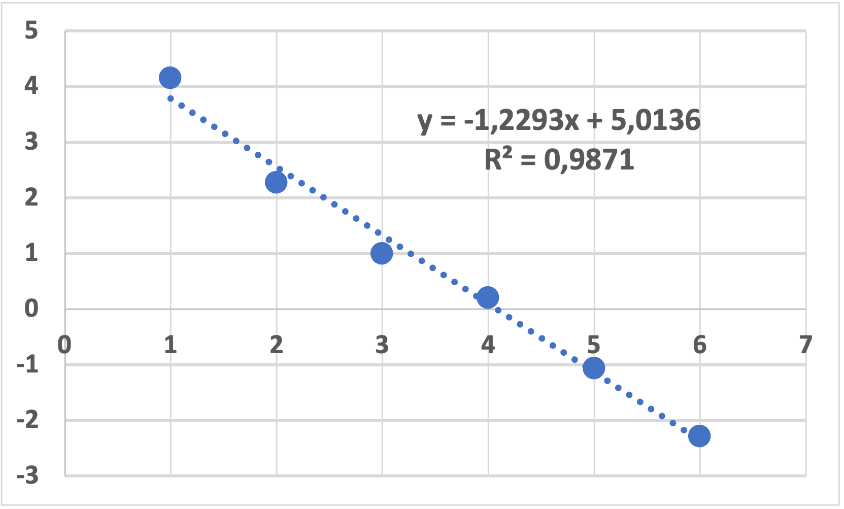
Figure 1: Error $\log_{2}\textrm{MSE}(\textbf{l},10)$ plotted against $\textbf{l}=1,...,6$.

References

- [1] Agarwal, A. and Pagliarani, S. (2021). A Fourier-based Picard-iteration approach for a class of McKean-Vlasov SDEs with Lévy jumps, Stochastics, 93(4), 592-624.
- [2] Applebaum, D. (2009). Lévy processes and stochastic calculus, volume 116 of Cambridge Studies in Advanced Mathematics, Cambridge University Press, Cambridge, Second edition.
- [3] Bossy, M. and Talay, D. (1997). A stochastic particle method for the McKean-Vlasov and the Burgers equation, Math. Comp., 66(217), 157–192.
- [4] Carmona, R. (2016). Lectures of BSDEs, Stochastic Control, and Stochastic Differential Games with Financial Applications, SIAM.
- [5] Carmona, R. and Delarue, F. (2018). Probabilistic theory of mean field games with applications I: Mean field FBSDEs, control, and games, Springer International Publishing, Switzerland.
- [6] Chen, X. and Gonçalo dos Reis (2022). A flexible split-step scheme for solving McKean-Vlasov stochastic differential equations, Applied Mathematics and Computation, 427, 127180.
- [7] dos Reis, G., Engelhardt, S. and Smith, G. (2022). Simulation of McKean-Vlasov SDEs with super-linear growth, IMA Journal of Numerical Analysis, 42, 874–922.
- [8] Erny, X. (2022). Well-posedness and propagation of chaos for McKean-Vlasov equations with jumps and locally Lipschitz coefficients, Stochastic Processes and their Applications, 150, 192–214.
- [9] Erny, X., Löcherbach, E. and Loukianova, D. (2022). White-noise driven conditional McKean-Vlasov limits for systems of particles with simultaneous and random jumps, Probability Theory and Related Fields, 183(3-4), 1027–1073.
- [10] Fang, W. and Giles, M.B. (2020). Adaptive Euler-Maruyama method for SDEs with non-globally Lipschitz drift, Ann. Appl. Probab., 30(2), 526–560.
- [11] Forien, R. and Pardoux, É. (2022). Household epidemic models and McKean-Vlasov Poisson driven stochastic differential equations, The Annals of Applied Probability, 32(2), 1210-1233.
- [12] Graham, C. (1992). McKean-Vlasov Itô-Skorohod equations, and nonlinear diffusions with discrete jump sets, Stochastic processes and their applications, 40(1), 69-82.
- [13] Hutzenthaler, M., Jentzen, A. and Kloeden, P. E. (2011). Strong and weak divergence in finite time of Euler’s method for stochastic differential equations with non-globally Lipschitz continuous coefficients, Proceedings of the Royal Society A: Mathematical, Physical and Engineering Sciences, 467(2130), 1563-1576.
- [14] Hutzenthaler, M., Jentzen, A. and Kloeden, P.E. (2012). Strong convergence of an explicit numerical method for SDEs with nonglobally Lipschitz continuous coefficients, Ann. Appl. Probab., 22 (4) 1611–1641.
- [15] Hutzenthaler, M., Kruse, T. and Nguyen, T.A. (2022), Multilevel Picard approximations for McKean-Vlasov stochastic differential equations, J. Math. Anal. Appl., 507, no. 1, Paper No. 125761, 14 pp.
- [16] Kieu, T. T., Luong, D. T. and Ngo, H. L. (2022). Tamed-adaptive Euler-Maruyama approximation for SDEs with locally Lipschitz continuous drift and locally Hölder continuous diffusion coefficients, Stochastic Analysis and Applications, 40(4), 714–734.
- [17] Kieu, TT., Luong, DT., Ngo, HL. and Tran, N.K. (2022). Strong convergence in infinite time interval of tamed-adaptive Euler-Maruyama scheme for Lévy-driven SDEs with irregular coefficients, Comp. Appl. Math., 41, 301.
- [18] Kohatsu-Higa, A. and Ogawa, S. (1997). Weak rate of convergence for an Euler scheme of nonlinear SDE’s, Monte Carlo Methods Appl., 3(4), 327–345.
- [19] Kumar, C. and Neelima (2021). On explicit Milstein-type scheme for McKean-Vlasov stochastic differential equations with super-linear drift coefficient, Electron. J. Probab., 26, Paper No. 111, 32 pp.
- [20] Kumar, C., Neelima, Reisinger, C. and Stockinger, W. (2022). Well-posedness and tamed schemes for McKean-Vlasov equations with common noise, Annals of Applied Probability, 32(5), 3283–3330.
- [21] Kumar, C. and Sabanis, S. (2017). On explicit approximations for Lévy driven SDEs with super-linear diffusion coefficients, Electron. J. Probab., 22(73), 1–19.
- [22] Liu, H., Shi, B. and Wu, F. (2023). Tamed Euler-Maruyama approximation of McKean-Vlasov stochastic differential equations with super-linear drift and Hölder diffusion coefficients, Appl. Numer. Math., 183, 56–85.
- [23] Liu, H., Wu, F. and Wu, M. (2023). The tamed Euler-Maruyama approximation of Mckean-Vlasov stochastic differential equations and asymptotic error analysis, Discrete Contin. Dyn. Syst. Ser. S, 16, no. 5, 1014–1040.
- [24] Mao, X. (2015). The truncated Euler-Maruyama method for stochastic differential equations, J. Comput. Appl. Math., 290, 370-384.
- [25] Mao, X., Szpruch, L. (2013) Strong convergence and stability of implicit numerical methods for stochastic differential equations with non-globally Lipschitz continuous coefficients, J. Comput. Appl. Math., 238 (15) 14–28 .
- [26] McKean, H. (1966). A class of Markov processes associated with nonlinear parabolic equations, Proceedings of the National Academy of Sciences of the USA, 56(6), 1907–1911.
- [27] Neelima, Biswas, S., Kumar, C., Gonçalo dos Reis and Reisinger, C. (2020). Well-posedness and tamed Euler schemes for McKean-Vlasov equations driven by Lévy noise. arXiv:2010.08585.
- [28] Ogawa, S. (1995). Some problems in the simulation of nonlinear diffusion processes, Mathematics and Computers in Simulation, 38(1-3), 217–-223.
- [29] Reisinger, C. and Stockinger, W. (2022). An adaptive Euler-Maruyama scheme for McKean-Vlasov SDEs with super-linear growth and application to the mean-field FitzHugh-Nagumo model, Journal of Computational and Applied Mathematics, 400, 113725.
- [30] Revuz, D. and Yor, M. (1999). Continuous martingales and Brownian motion, Vol. 293. Springer Science & Business Media.
- [31] Sabanis, S. (2013). A note on tamed Euler approximations, Electron. Commun. Probab., 18, 1–10.
- [32] Sabanis, S. (2016). Euler approximations with varying coefficients: the case of superlinear growing diffusion coefficients, Ann. Appl. Probab, 26(4), 2083–2105.
- [33] Zhu, J., Brzezniak, Z. and Liu, W. (2019). Maximal inequalities and exponential estimates for stochastic convolutions driven by Lévy-type processes in Banach spaces with application to stochastic quasi-geostrophic equations, SIAM Journal on Mathematical Analysis, 51(3), 2121-2167.