Well-balanced convex limiting for finite element discretizations of steady convection-diffusion-reaction equations

Abstract

We address the numerical treatment of source terms in algebraic flux correction schemes for steady convection-diffusion-reaction (CDR) equations. The proposed algorithm constrains a continuous piecewise-linear finite element approximation using a monolithic convex limiting (MCL) strategy. Failure to discretize the convective derivatives and source terms in a compatible manner produces spurious ripples, e.g., in regions where the coefficients of the continuous problem are constant and the exact solution is linear. We cure this deficiency by incorporating source term components into the fluxes and intermediate states of the MCL procedure. The design of our new limiter is motivated by the desire to preserve simple steady-state equilibria exactly, as in well-balanced schemes for the shallow water equations. The results of our numerical experiments for two-dimensional CDR problems illustrate potential benefits of well-balanced flux limiting in the scalar case.

Keywords: convection-diffusion-reaction equations; discrete maximum principles; positivity preservation; algebraic flux correction; monolithic convex limiting; well-balanced schemes

1 Introduction

Many modern numerical schemes for conservation laws are equipped with flux or slope limiters that ensure the validity of discrete maximum principles. A comprehensive review of such algorithms and of the underlying theory can be found, e.g., in [13]. Matters become more complicated in the case of inhomogeneous balance laws, especially if strong consistency with some steady-state solutions is desired. Discretizations that provide such consistency are called well balanced in the literature [2, 6, 17]. For example, a well-balanced scheme for the system of shallow water equations (SWEs) should preserve at least lake-at-rest equilibria (zero velocity, constant free surface elevation). In general, sources/sinks should be discretized in a manner compatible with the numerical treatment of flux terms [14]. In the one-dimensional case, proper balancing can often be achieved by discretizing a ‘homogeneous form’ of the balance law [5, 7, 19]. The design of well-balanced schemes for multidimensional problems is usually more difficult, especially if the source term does not admit a natural representation as the gradient of a scalar potential or divergence of a vector field.

A well-balanced and positivity-preserving finite element scheme for the inhomogeneous SWE system was developed by Hajduk [8] using the framework of algebraic flux correction. The monolithic convex limiting (MCL) algorithm presented in [8, 9] incorporates discretized bathymetry gradients into the numerical fluxes and intermediate states of the spatial semi-discretization. In the present paper, we show that the source term of a scalar convection-diffusion-reaction problem can be treated similarly. In particular, we define numerical fluxes that ensure consistency of the well-balanced MCL approximation with a linear steady state. Using a convex decomposition into intermediate states, we enforce positivity preservation, as well as local and global discrete maximum principles.

In Section 2, we discretize a model problem using the standard continuous Galerkin finite element method. The algorithm presented in Section 3 stabilizes the convective part using the MCL methodology for hyperbolic conservation laws [12, 13]. The discretization of source terms is left unchanged in this version. Our well-balanced generalization is derived in Section 4, analyzed in Section 5, and tested numerically in Section 6. The numerical examples with locally linear exact solutions show that improper treatment of source terms may cause a flux-corrected finite element method to produce spurious ripples. The proposed approach provides an effective remedy to this problem. Section 7 closes the paper with a summary and discussion of the main findings.

2 Model problem and Galerkin discretization

In computational fluid dynamics, steady convection-diffusion-reaction (CDR) equations are often used to simulate distributions of scalar quantities of interest, such as temperature, energy, or concentration of chemical species. Let $d\in\{1,2,3\}$ denote the number of space dimensions. Choosing a domain $\Omega\subset\mathbb{R}^{d}$ with Lipschitz boundary $\Gamma=\partial\Omega$, we consider the Dirichlet problem

$$-\varepsilon\Delta u+\mathbf{v}\cdot\nabla u+c\,u =f \quad\mathrm{in}\ \ \Omega,$$ (1a)

$$u =u_{D}\ \quad\mathrm{on}\ \ \Gamma_{D},$$ (1b)

where $u=u(\mathbf{x})$ is the unknown variable, $\varepsilon\geq 0$ is a constant diffusion coefficient, $\mathbf{v}=\mathbf{v}(\mathbf{x})$ is a given velocity field, $c=c(\mathbf{x})$ is a nonnegative reaction rate, and $f=f(\mathbf{x})$ is a general source term depending on the vector $\mathbf{x}=(x_{1},\ldots,x_{d})^{\top}$ of space coordinates. In the case $\varepsilon>0$, the Dirichlet boundary data $u_{D}$ is prescribed on $\Gamma_{D}=\Gamma$. In the case $\varepsilon=0$, equation (1a) becomes hyperbolic and, therefore, condition (1b) is imposed only on the inflow boundary $\Gamma_{D}\subseteq\Gamma$.

We are particularly interested in the case of dominating convection. Thus we assume that $\|\mathbf{v}\|_{(L^{\infty}(\Omega))^{d}}\gg\frac{\varepsilon}{L}$, where $L$ is the characteristic length of the problem. Because of this assumption, an exact solution to (1) may exhibit interior and/or boundary layers, in which the gradients are steep and standard finite element methods may violate discrete maximum principles [18].

Let $\mathcal{T}_{h}$ be a conforming simplex mesh such that $\bigcup_{K\in\mathcal{T}_{h}}K=\overline{\Omega}$. The vertices of $\mathcal{T}_{h}$ are denoted by $\mathbf{x}_{j},\ j\in\{1,\ldots,N_{h}\}$ and the maximum diameter of mesh cells $K\in\mathcal{T}_{h}$ by $h>0$. Restricting our discussion to linear finite elements in this paper, we express numerical approximations

$$u_{h}=\sum_{j=1}^{N_{h}}u_{j}\varphi_{j}$$ (2)

in terms of Lagrange basis functions $\varphi_{j}\in C(\bar{\Omega}),\ j\in\{1,\ldots,N_{h}\}$ such that $\varphi_{j}|_{K}\in\mathbb{P}_{1}(K)\ \forall K\in\mathcal{T}_{h}$ and $\varphi_{j}(\mathbf{x}_{i})=\delta_{ij}$ for $i\in\{1,\ldots,N_{h}\}$. The corresponding finite element space is denoted by $V_{h}$.

We assume that the Dirichlet boundary nodes are numbered using indices $M_{h}+1,\ldots,N_{h}$. Substituting (2) into the discretized weak form

$$\int_{\Omega}\left(\varepsilon\nabla w_{h}\cdot\nabla u_{h}+w_{h}[\mathbf{v}\cdot\nabla u_{h}+c\,u_{h}]\right)\mathrm{d}\mathbf{x}=\int_{\Omega}w_{h}f\mathrm{d}\mathbf{x}$$

of (1a) and using test functions $w_{h}\in\{\varphi_{1},\dots,\varphi_{M_{h}}\}$, we obtain a linear system for the unknown nodal values:

$$\sum_{j=1}^{N_{h}}(a_{ij}^{D}+a_{ij}^{C}+a_{ij}^{R})u_{j} =b_{i}, i=1,\ldots,M_{h},$$ (3a)

$$u_{i} =u_{D}(\mathbf{x}_{i}),\qquad i=M_{h}+1,\ldots,N_{h}.$$ (3b)

The coefficients of the involved matrices and vectors are given by

$$a_{ij}^{D} =\varepsilon\int_{\Omega}\nabla\varphi_{i}\cdot\nabla\varphi_{j}\mathrm{d}\mathbf{x},\qquad a_{ij}^{C}=\int_{\Omega}\varphi_{i}\mathbf{v}\cdot\nabla\varphi_{j}\mathrm{d}\mathbf{x},$$

$$a_{ij}^{R} =\int_{\Omega}c\,\varphi_{i}\varphi_{j}\mathrm{d}\mathbf{x},\qquad b_{i}=\int_{\Omega}\varphi_{i}f\mathrm{d}\mathbf{x}.$$

The matrices $A^{D}=(a_{ij}^{D})_{i,j=1}^{N_{h}},\ A^{C}=(a_{ij}^{C})_{i,j=1}^{N_{h}}$, and $A^{R}=(a_{ij}^{R})_{i,j=1}^{N_{h}}$ result from the discretization of the diffusive, convective, and reactive terms, respectively. The contribution of the right-hand side $f$ is represented by the vector $b=(b_{i})_{i=1}^{M_{h}}$ of discretized source terms.

In the next section, we stabilize the discrete convection operator $A^{C}$ using an algebraic flux correction scheme that satisfies a local discrete maximum principle (DMP) in the case $\varepsilon=0$. To ensure the DMP property of the discrete diffusion operator $A^{D}$ for $\varepsilon>0$, we assume that $a_{ij}^{D}\leq 0$ for $j\neq i\in\{1,\ldots,N_{h}\}$. This requirement is met for simplex meshes of weakly acute type [4].

3 Convex limiting for convective terms

Let $\mathcal{N}_{i}$ denote the set of indices $j$ such that the basis functions $\varphi_{i}$ and $\varphi_{j}$ have overlapping supports. For our purposes, it is worthwhile to write the $i$th equation of (3a) in the form

$$a_{i}^{R}u_{i}+\sum_{j\in\mathcal{N}_{i}\backslash\{i\}}(a_{ij}^{D}+a_{ij}^{C}+a_{ij}^{R})(u_{j}-u_{i})=b_{i},$$ (4)

where $a_{i}^{R}=\sum_{j\in\mathcal{N}_{i}}a_{ij}^{R}$ is a diagonal entry of the ‘lumped’ reactive mass matrix $\tilde{A}_{R}=(a_{i}^{R}\delta_{ij})_{i,j=1}^{N_{h}}$.

Introducing an artificial diffusion (graph Laplacian) operator $D=(d_{ij})_{i,j=1}^{N_{h}}$ with entries

$$d_{ij}=\begin{cases}\max\{|a_{ij}^{C}|,\delta h^{d-1},|a_{ji}^{C}|\}&\mbox{if}\ {j\in\mathcal{N}_{i}\backslash\{i\},}\\ {0}&{\mbox{if}\ j\not\in\mathcal{N}_{i},}\\ -\sum_{k\in\mathcal{N}_{i}\backslash\{i\}}d_{ik}&\mbox{if}\ j=i,\end{cases}$$

we define auxiliary bar states $\bar{u}_{ij}$ and numerical fluxes $f_{ij}$ for $j\in\mathcal{N}_{i}\backslash\{i\}$ as follows:

$$\bar{u}_{ij}=\frac{u_{j}+u_{i}}{2}-\frac{a_{ij}^{C}(u_{j}-u_{i})}{2d_{ij}},\qquad f_{ij}=(d_{ij}+a_{ij}^{R})(u_{i}-u_{j}).$$ (5)

It is easy to verify that the Galerkin discretization (4) is equivalent to

$$a_{i}^{R}u_{i}-\sum_{j\in\mathcal{N}_{i}\backslash\{i\}}[2d_{ij}(\bar{u}_{ij}-u_{i})+f_{ij}-a_{ij}^{D}(u_{j}-u_{i})]=b_{i}.$$ (6)

The monolithic convex limiting (MCL) algorithm developed in [12] for homogeneous hyperbolic problems replaces the target flux $f_{ij}=-f_{ji}$ with an approximation $f_{ij}^{*}=-f_{ji}^{*}$ such that

$$\min_{j\in\mathcal{N}_{i}}u_{j}=:u_{i}^{\min}\leq\bar{u}_{ij}^{*}:=\bar{u}_{ij}+\frac{f_{ij}^{*}}{2d_{ij}}\leq u_{i}^{\max}:=\max_{j\in\mathcal{N}_{i}}u_{j}.$$

These inequality constraints imply the validity of local DMPs and are satisfied for

$$f^{*}_{ij}=\begin{cases}\min\left\{f_{ij},\min\left\{2d_{ij}\left(u_{i}^{\max}-\bar{u}_{ij}\right),2d_{ij}\left(\bar{u}_{ji}-u_{j}^{\min}\right)\right\}\right\}&\text{if }f_{ij}>0,\\ 0&\text{if }f_{ij}=0,\\ \max\left\{f_{ij},\max\left\{2d_{ij}\left(u_{i}^{\min}-\bar{u}_{ij}\right),2d_{ij}\left(\bar{u}_{ji}-u_{j}^{\max}\right)\right\}\right\}&\text{if }f_{ij}<0.\end{cases}$$ (7)

To avoid division by $d_{ij}$ in the formula for $\bar{u}_{ij}$, the products $2d_{ij}\bar{u}_{ij}$ are calculated directly in practical implementations of (7). We refer the reader to [12, 13] for further explanations and proofs of local DMPs that are valid in the limit of pure convection (i.e., for $\varepsilon=0,\ c\equiv 0$, $f\equiv 0$).

4 Well-balanced convex limiting

As mentioned in the introduction, a well-designed numerical scheme should be consistent with simple steady-state equilibria. An exact solution of the CDR equation (1a) with

$$\varepsilon\geq 0,\quad\mathbf{v}\equiv\hat{\mathbf{v}},\quad c\equiv 0,\quad f\equiv\hat{f},$$ (8)

where $\hat{\mathbf{v}}\in\mathbb{R}^{d}\backslash\{\mathbf{0}\}$ and $\hat{f}\in\mathbb{R}\backslash\{0\}$ are constant, is given by

$$\hat{u}(\mathbf{x})=\hat{f}\ \frac{\mathbf{x}\cdot\hat{\mathbf{v}}}{|\hat{\mathbf{v}}|^{2}}.$$ (9)

We denote by $|\cdot|$ the Euclidean norm of vectors in $\mathbb{R}^{d}$. By the linearity of $\hat{u}$, we have

$$\hat{\mathbf{v}}\cdot\nabla\hat{u}-\varepsilon\Delta\hat{u}=\hat{\mathbf{v}}\cdot\nabla\hat{u}=\hat{f}.$$

The equilibrium state $\hat{u}$ is preserved exactly by the standard Galerkin discretization because the linear function $\hat{u}(\mathbf{x})$ belongs to the space $V_{h}$. However, this desirable property may be lost if an algebraic stabilization of convective terms is not balanced by an appropriate modification of $b_{i}$.

To derive a well-balanced MCL scheme for problem (1) with velocity $\mathbf{v}=\mathbf{v}(\mathbf{x})$ such that

$$|\mathbf{v}(\mathbf{x}_{i})|+|\mathbf{v}(\mathbf{x}_{j})|>0,\qquad i=1,\dots,N_{h},\quad j\in\mathcal{N}_{i}\backslash\{i\},$$

we introduce the balancing fluxes

$$P_{ij}=\frac{1}{2}\frac{s_{i}+s_{j}}{2}\frac{(\mathbf{x}_{i}-\mathbf{x}_{j})\cdot(\mathbf{v}(\mathbf{x}_{i})+\mathbf{v}(\mathbf{x}_{j}))}{2\,\left(\max\{|\mathbf{v}(\mathbf{x}_{i})|,|\mathbf{v}(\mathbf{x}_{j})|\}\right)^{2}},\qquad i=1,\dots,N_{h},\quad j\in\mathcal{N}_{i}\backslash\{i\}.$$ (10)

In this formula, $s_{i}:=f(\mathbf{x}_{i})-c(\mathbf{x}_{i})u_{i}$ is the net source term of the CDR equation (1a) evaluated at the vertex $\mathbf{x}_{i}$. We replace the bar state $\bar{u}_{ij}$ of representation (6) with (cf. [9])

$$\bar{u}_{ij}^{s}=\bar{u}_{ij}+\alpha_{ij}P_{ij}+\frac{b_{i}}{a_{i}^{C}},\qquad{i=1,\dots,M_{h},\quad j\in\mathcal{N}_{i}\backslash\{i\},}$$

where $a_{i}^{C}=\sum_{j\in\mathcal{N}_{i}\backslash\{i\}}2d_{ij}$ and $\alpha_{ij}=\alpha_{ji}$ is a correction factor to be defined below. By definition of $d_{ij}$, the coefficient $a_{i}^{C}$ is strictly positive. Hence, no division by zero can occur.

The standard Galerkin discretization (4) can now be expressed in terms of $\bar{u}_{ij}^{s}$ and

$$f_{ij}^{s}=2d_{ij}\left[\frac{u_{i}-u_{j}}{2}-\alpha_{ij}P_{ij}\right]+a_{ij}^{R}(u_{i}-u_{j})$$ (11)

as follows:

$$a_{i}^{R}u_{i}-\sum_{j\in\mathcal{N}_{i}\backslash\{i\}}[2d_{ij}(\bar{u}_{ij}^{s}-u_{i})+f_{ij}^{s}-a_{ij}^{D}(u_{j}-u_{i})]=0.$$ (12)

Note that we have distributed the source term $b_{i}$ among the bar states $\bar{u}_{ij}^{s}$ and stabilized these intermediate states using the limited balancing fluxes $\alpha_{ij}P_{ij}$. A similar algebraic splitting was used in [8, 9] to construct a well-balanced MCL scheme for the SWE system. Our definition of $f_{ij}^{s}$ ensures that $f_{ij}^{s}=0$ if the coefficients of problem (1) are given by (8), $u_{h}=\hat{u}$, and $\alpha_{ij}=1$. This enables us to preserve strong consistency at the corresponding steady state (see Remark 4 below).

Figure 1: Fictitious nodes.

To design an algorithm that produces $\alpha_{ij}=1$ for $u_{h}=\hat{u}$ given by formula (9), we introduce fictitious nodes $\mathbf{x}^{i}_{j}$ which are placed symmetrically to the nodes $\mathbf{x}_{j}$, $j\in\mathcal{N}_{i}\backslash\{i\}$ with respect to $\mathbf{x}_{i}$, i.e., $(\mathbf{x}^{i}_{j}+\mathbf{x}_{j})/2=\mathbf{x}_{i}$; see Fig. 1. We denote by $u^{i}_{j}$ the (fictitious) value of $u_{h}$ at $\mathbf{x}^{i}_{j}$. If the fictitious node is contained in one of the mesh cells containing $\mathbf{x}_{i}$ (like the node $\mathbf{x}^{i}_{k}$ in Fig. 1), then we simply evaluate $u_{h}$ at this point. If this is not the case, then following [11] we denote by $K^{i}_{j}$ a mesh cell containing $\mathbf{x}_{i}$ that is intersected by the half line $\{\mathbf{x}_{i}+\theta\,(\mathbf{x}_{i}-\mathbf{x}_{j})\,:\,\,\theta>0\}$ (cf. Fig. 1), extend $u_{h}|_{K^{i}_{j}}$ to a first degree polynomial on $\mathbb{R}^{d}$ and evaluate this extension at $\mathbf{x}^{i}_{j}$. Thus, in both cases, we obtain

$$u^{i}_{j}=u_{i}+\nabla u_{h}|_{K^{i}_{j}}\cdot(\mathbf{x}^{i}_{j}-\mathbf{x}_{i})=u_{i}+\nabla u_{h}|_{K^{i}_{j}}\cdot(\mathbf{x}_{i}-\mathbf{x}_{j}).$$ (13)

Other definitions of values at fictitious nodes can be found e.g. in [1, 16, 3].

Remark 1.

If $|\mathbf{v}(\mathbf{x}_{i})|+|\mathbf{v}(\mathbf{x}_{j})|$ is small, then the magnitude of $P_{ij}$ may become large. In (11) and (12), this is compensated by the multiplication by $d_{ij}$ that depends on $\mathbf{v}$.

Let us now proceed to formulating appropriate inequality constraints for well-balanced flux limiting. The multiplication by the correction factor $\alpha_{ij}=\alpha_{ji}$ in the formula for the flux $f_{ij}^{s}=-f_{ji}^{s}$ makes it possible to enforce the local discrete maximum principles

$$u_{i}=u_{i}^{\max}\ \,\wedge\ \, b_{i}\leq 0\quad\Rightarrow\quad\bar{u}_{ij}^{s}\leq\max\{u_{i},u_{j}\}{\quad\forall\,\,j\in\mathcal{N}_{i}\backslash\{i\},}$$ (14a)

$$u_{i}=u_{i}^{\min}\ \,\wedge\ \, b_{i}\geq 0\quad\Rightarrow\quad\bar{u}_{ij}^{s}\geq\min\{u_{i},u_{j}\}{\quad\forall\,\,j\in\mathcal{N}_{i}\backslash\{i\},}$$ (14b)

for $i=1,\dots,M_{h}$. Adopting this design criterion, we use the auxiliary quantities

$$\begin{array}[]{l}\displaystyle Q_{ij}^{+}=\max\left\{\frac{u^{i}_{j}-u_{i}}{2},\max\{u_{i},u_{j}\}-\bar{u}_{ij}-\frac{b_{i}}{a_{i}^{C}}\right\},\\[14.22636pt] \displaystyle Q_{ij}^{-}=\min\left\{\frac{u^{i}_{j}-u_{i}}{2},\min\{u_{i},u_{j}\}-\bar{u}_{ij}-\frac{b_{i}}{a_{i}^{C}}\right\},\end{array}\qquad i=1,\dots,M_{h},\quad j\in\mathcal{N}_{i}\backslash\{i\}$$

to define

$$R_{ij}=\begin{cases}\displaystyle\frac{Q_{ij}^{+}}{P_{ij}}&\mbox{if}\ b_{i}\leq 0\ \mbox{and}\ P_{ij}>Q_{ij}^{+},\\[8.53581pt] \displaystyle\frac{Q_{ij}^{-}}{P_{ij}}&\mbox{if}\ b_{i}\geq 0\ \mbox{and}\ P_{ij}<Q_{ij}^{-},\\[8.53581pt] 1&\mbox{otherwise},\end{cases}\qquad{i=1,\dots,M_{h},\quad j\in\mathcal{N}_{i}\backslash\{i\}.}$$

Furthermore, we set

$$R_{ij}=1,\qquad i=M_{h}+1,\dots,N_{h},\quad j\in\mathcal{N}_{i}\backslash\{i\}.$$

Then we define

$$\alpha_{ij}=\min\{R_{ij},R_{ji}\},\qquad{i=1,\dots,N_{h},\quad j\in\mathcal{N}_{i}\backslash\{i\}.}$$

This limiting strategy yields $\alpha_{ij}\in[0,1]$ such that $\alpha_{ij}=\alpha_{ji}$ and conditions (14) are satisfied.

Remark 2.

In (14), both $\max\{u_{i},u_{j}\}$ and $\min\{u_{i},u_{j}\}$ are equal to $u_{i}$ but we use the present formulation to establish a correspondence to the definition of $Q_{ij}^{\pm}$. Note that, under the sign conditions on $b_{i}$, the left-hand side inequalities of (14) hold not only under the assumption that $u_{i}$ is a local maximum or minimum, but also when $(u^{i}_{j}-u_{i})/2$ is dominated by the second term in the definition of $Q_{ij}^{+}$ or $Q_{ij}^{-}$. In particular, this is the case if $u^{i}_{j}-u_{i}$ has the same sign as $b_{i}$. Replacing $\max\{u_{i},u_{j}\}$ and $\min\{u_{i},u_{j}\}$ by $u_{i}$ in the definitions of $Q_{ij}^{\pm}$ and in (14) would be too restrictive since then the left-hand side inequalities of (14) would hold for a much smaller class of functions.

In a practical implementation, we calculate the limited balancing fluxes

$$\alpha_{ij}P_{ij}=\mathrm{sgn}(P_{ij})\min\{R_{ij}|P_{ij}|,R_{ji}|P_{ji}|\},\qquad{i=1,\dots,N_{h},\quad j\in\mathcal{N}_{i}\backslash\{i\}}$$ (15)

directly to avoid possible division by zero in finite precision arithmetic. Note that $Q_{ij}^{+}\geq 0$ if $b_{i}\leq 0$ and $Q_{ij}^{-}\leq 0$ if $b_{i}\geq 0$. It follows that

$$R_{ij}|P_{ij}|=\begin{cases}\mathrm{sgn}(P_{ij})\min\{P_{ij},Q_{ij}^{+}\}&\mbox{if}\ b_{i}<0\ \mbox{or}\ (b_{i}=0\ \mbox{and}\ P_{ij}\geq 0),\\ \mathrm{sgn}(P_{ij})\max\{P_{ij},Q_{ij}^{-}\}&\mbox{if}\ b_{i}>0\ \mbox{or}\ (b_{i}=0\ \mbox{and}\ P_{ij}\leq 0)\end{cases}$$ (16)

for $i=1,\dots,M_{h}$ and $j\in\mathcal{N}_{i}\backslash\{i\}$.

In the context of scalar CDR problems, we define the limited approximation

$$f_{ij}^{s,*}=\begin{cases}\min\left\{f_{ij}^{s},\min\left\{2d_{ij}\left(\bar{u}_{i}^{\max}-\bar{u}_{ij}^{s}\right),2d_{ij}\left(\bar{u}_{ji}^{s}-\bar{u}_{j}^{\min}\right)\right\}\right\}&\text{if }f_{ij}^{s}>0,\\ 0&\text{if }f_{ij}^{s}=0,\\ \max\left\{f_{ij}^{s},\max\left\{2d_{ij}\left(\bar{u}_{i}^{\min}-\bar{u}_{ij}^{s}\right),2d_{ij}\left(\bar{u}_{ji}^{s}-\bar{u}_{j}^{\max}\right)\right\}\right\}&\text{if }f_{ij}^{s}<0\end{cases}$$ (17)

to $f_{ij}^{s}$ using the low-order bar states $\bar{u}_{ij}^{s}$ to construct the local bounds

$$\bar{u}_{i}^{\min}:=\min_{j\in\mathcal{N}_{i}\backslash\{i\}}\bar{u}_{ij}^{s},\qquad\bar{u}_{i}^{\max}:=\max_{j\in\mathcal{N}_{i}\backslash\{i\}}\bar{u}_{ij}^{s}.$$

This limiting strategy ensures that the flux-corrected intermediate states

$$\bar{u}_{ij}^{s,*}=\bar{u}_{ij}^{s}+\frac{f_{ij}^{s,*}}{2d_{ij}}$$

satisfy the inequality constraints

$$\bar{u}_{i}^{\min}\leq\bar{u}_{ij}^{s,*}\leq\bar{u}_{i}^{\max}.$$ (18)

Note that (17) is well defined only if both indices $i$ and $j$ refer to interior nodes (and $j\in\mathcal{N}_{i}\backslash\{i\}$ as usual). If $i\in\{1,\dots,M_{h}\}$ and $j\in\mathcal{N}_{i}\cap\{M_{h}+1,\dots,N_{h}\}$, we set

$$f_{ij}^{s,*}=\begin{cases}\min\left\{f_{ij}^{s},2d_{ij}\left(\bar{u}_{i}^{\max}-\bar{u}_{ij}^{s}\right)\right\}&\text{if }f_{ij}^{s}>0,\\ 0&\text{if }f_{ij}^{s}=0,\\ \max\left\{f_{ij}^{s},2d_{ij}\left(\bar{u}_{i}^{\min}-\bar{u}_{ij}^{s}\right)\right\}&\text{if }f_{ij}^{s}<0.\end{cases}$$ (19)

This again guarantees that the constraints (18) hold.

Our well-balanced MCL scheme for problem (1) can be written in the ‘homogeneous’ form

$$a_{i}^{R}u_{i}-\sum_{j\in\mathcal{N}_{i}\backslash\{i\}}[2d_{ij}(\bar{u}_{ij}^{s,*}-u_{i})-a_{ij}^{D}(u_{j}-u_{i})] =0, {i=1,\dots,M_{h},}$$ (20a)

$${u_{i}} {=u_{D}(\mathbf{x}_{i}),}\qquad {i=M_{h}+1,\dots,N_{h}},$$ (20b)

in which the source terms are incorporated into the bar states $\bar{u}_{ij}^{s,*}$ (similarly to [8, 9]).

Remark 3.

In practice, $u_{i}$ can be calculated using the bound-preserving fixed-point iteration

$$u_{i}^{n+1}=\frac{1}{a_{i}}\sum_{j\in\mathcal{N}_{i}\backslash\{i\}}[2d_{ij}\bar{u}_{ij}^{s,*,n}-a_{ij}^{D}u_{j}^{n}],$$

where $a_{i}=a_{i}^{R}+a_{i}^{C}-\sum_{j\in\mathcal{N}_{i}\backslash\{i\}}a_{ij}^{D}>0$. Each update produces a linear combination of the states that appear on the right-hand side. In view of our assumption that $a_{ij}^{D}\leq 0$ for $j\neq i$, all weights are nonnegative. Moreover, they add up to unity if $a_{i}^{R}=0$.

Remark 4.

If the coefficients of problem (1) are given by (8), then $s_{i}=s_{j}=\hat{f}$. Moreover, $c\equiv 0$ implies $a_{ij}^{R}=0$. Substituting the nodal values $u_{i}=\hat{u}(\mathbf{x}_{i})$ of the exact steady-state solution (9) into the definition (10) of the balancing flux, we find that $P_{ij}=(u_{i}-u_{j})/2$. In addition, since $u_{h}$ is a first degree polynomial in $\Omega$, one has $u^{i}_{j}-u_{i}=u_{i}-u_{j}$ due to (13). Hence, by definition of $Q_{ij}^{\pm}$, it follows that $\alpha_{ij}=1$ and $f_{ij}^{s}=0=f_{ij}^{s,*}$. Therefore, the flux-corrected scheme (20a) coincides with the equilibrium-preserving Galerkin discretization (12). This proves that (20a) is well balanced.

Remark 5.

To avoid the evaluation of $u_{h}$ at fictitious nodes, a simplified version of the above algorithm calculates the correction factors $\alpha_{ij}$ using

$$Q_{ij}^{+}=\max\{u_{i},u_{j}\}-\bar{u}_{ij}-\frac{b_{i}}{a_{i}^{C}},\qquad Q_{ij}^{-}=\min\{u_{i},u_{j}\}-\bar{u}_{ij}-\frac{b_{i}}{a_{i}^{C}},$$

for $i=1,\dots,M_{h}$, $j\in\mathcal{N}_{i}\backslash\{i\}$. Then, instead of (14), one has the stronger properties

$$b_{i}\leq 0\quad\Rightarrow\quad\bar{u}_{ij}^{s}\leq\max\{u_{i},u_{j}\}\quad\forall\,\,j\in\mathcal{N}_{i}\backslash\{i\},$$

$$b_{i}\geq 0\quad\Rightarrow\quad\bar{u}_{ij}^{s}\geq\min\{u_{i},u_{j}\}\quad\forall\,\,j\in\mathcal{N}_{i}\backslash\{i\},$$

for $i=1,\dots,M_{h}$. The theoretical results that we prove in the next section remain valid. However, the assertion of Remark 4 is not true in general any more for this version of MCL. Nevertheless, one can still prove that the scheme (20a) is well balanced on some types of uniform meshes. On general meshes, the scheme may be not well balanced, as numerical experiments show.

5 Solvability and discrete maximum principle

In this section, we investigate the solvability of the nonlinear problem (20) and the validity of local and global discrete maximum principles. All results will be proven under the assumption that $\varepsilon>0$. To prove the solvability, additional assumptions on the data will be made as well.

First we cast (20a) into a form that will be convenient for our analysis. It follows from (5) that

$$d_{ij}(u_{i}-u_{j})=2d_{ij}(u_{i}-\bar{u}_{ij})+a_{ij}^{C}(u_{i}-u_{j})\,.$$ (21)

Substituting (21) into (11), one obtains

$$f_{ij}^{s}=2d_{ij}(u_{i}-\bar{u}_{ij}^{s})+(a_{ij}^{C}+a_{ij}^{R})(u_{i}-u_{j})+2d_{ij}\frac{b_{i}}{a_{i}^{C}}.$$ (22)

Using this expression, it is easy to verify that (20a) can be equivalently written in the form

$$a_{i}^{R}u_{i}+\sum_{j\in\mathcal{N}_{i}\backslash\{i\}}(a_{ij}^{D}+a_{ij}^{C}+a_{ij}^{R})(u_{j}-u_{i})+\sum_{j\in\mathcal{N}_{i}\backslash\{i\}}(f_{ij}^{s}-f_{ij}^{s,*})=b_{i},\quad i=1,\dots,M_{h}.$$ (23)

The solvability proof will be based on the following consequence of the Brouwer fixed-point theorem.

Lemma 1.

Let $X$ be a finite-dimensional Hilbert space with inner product $(\cdot,\cdot)_{X}$ and norm $\|\cdot\|_{X}$. Let $T:X\to X$ be a continuous mapping and $K>0$ a real number such that $(Tx,x)_{X}>0$ for any $x\in X$ with $\|x\|_{X}=K$. Then there exists $x\in X$ such that $\|x\|_{X}\leq K$ and $Tx=0$.

Proof.

See [20, p. 164, Lemma 1.4]. ∎

Theorem 1.

Let the data of (1) satisfy $\varepsilon>0$, $\nabla\cdot\mathbf{v}=0$, and $c\equiv 0$. Then the nonlinear problem (20) has a solution.

Proof.

The fluxes $f_{ij}^{s}$ and $f_{ij}^{s,*}$ are functions of the coefficient vectors $u:=(u_{1},\dots,u_{N_{h}})^{\top}\in{\mathbb{R}}^{N_{h}}$. Let us first investigate whether they depend on $u$ in a continuous way. We will proceed step by step. To show that the bar states $\bar{u}_{ij}^{s}$ are continuous functions of $u$, it suffices to investigate the continuity of (15). Since minimum and maximum are continuous functions, the functions $Q_{ij}^{+}$ and $Q_{ij}^{-}$ are continuous. If $\bar{u}\in{\mathbb{R}}^{N_{h}}$ is such that $P_{ij}(\bar{u})\neq 0$, then $P_{ij}\neq 0$ in a neighborhood of $\bar{u}$ and hence $R_{ij}|P_{ij}|$ and $R_{ji}|P_{ji}|$ are continuous in this neighborhood in view of (16). Thus, $\alpha_{ij}P_{ij}$ is continuous at $\bar{u}$ due to (15). Moreover, if $P_{ij}(\bar{u})=0$, one obtains

$$\left|(\alpha_{ij}P_{ij})(u)-(\alpha_{ij}P_{ij})(\bar{u})\right|=|\alpha_{ij}P_{ij}|(u)\leq|P_{ij}(u)|=|P_{ij}(u)-P_{ij}(\bar{u})|$$ (24)

so that $\alpha_{ij}P_{ij}$ is continuous at $\bar{u}$ also in this case. Therefore, the function in (15) is continuous on ${\mathbb{R}}^{N_{h}}$. Consequently, $\bar{u}_{ij}^{s}$, $f_{ij}^{s}$, $\bar{u}_{i}^{\min}$, and $\bar{u}_{i}^{\max}$ are continuous on ${\mathbb{R}}^{N_{h}}$. Then, if $f_{ij}^{s}(\bar{u})\neq 0$ for some $\bar{u}\in{\mathbb{R}}^{N_{h}}$, it follows from (17) and (19) that $f_{ij}^{s,*}$ is continuous in a neighborhood of $\bar{u}$. If $f_{ij}^{s}(\bar{u})=0$, then the continuity of $f_{ij}^{s,*}$ at $\bar{u}$ follows as in (24) since $|f_{ij}^{s,*}|\leq|f_{ij}^{s}|$ due to (17) and (19).

A coefficient vector $u=(u_{1},\dots,u_{N_{h}})^{\top}$ solving (20) can be split into the vectors $u_{\rm I}:=(u_{1},\dots,u_{M_{h}})^{\top}$ and $u_{\rm B}:=(u_{M_{h}+1},\dots,u_{N_{h}})^{\top}=(u_{D}(\mathbf{x}_{M_{h}+1}),\dots,u_{D}(\mathbf{x}_{N_{h}}))^{\top}$. Let us define a mapping $T:{\mathbb{R}}^{M_{h}}\to{\mathbb{R}}^{M_{h}}$ by

$$(Tv)_{i}=\sum_{j=1}^{M_{h}}(a_{ij}^{D}+a_{ij}^{C}+a_{ij}^{R})v_{j}+\sum_{j\in\mathcal{N}_{i}\backslash\{i\}}(f_{ij}^{s}-f_{ij}^{s,*})(v,u_{\rm B})-g_{i},\quad i=1,\dots,M_{h},\quad v\in{\mathbb{R}}^{M_{h}},$$

where

$$g_{i}=b_{i}-\sum_{j=M_{h}+1}^{N_{h}}(a_{ij}^{D}+a_{ij}^{C}+a_{ij}^{R})u_{D}(\mathbf{x}_{j}),\quad i=1,\dots,M_{h}.$$

Then $T$ is continuous and, since (20a) and (23) are equivalent, a vector $u\in{\mathbb{R}}^{N_{h}}$ satisfying (20b) solves (20a) if and only if $Tu_{\rm I}=0$. Thus, in view of Lemma 1, to prove the solvability of (20), it suffices to analyze the product $(Tv,v)$, where $(\cdot,\cdot)$ denotes the Euclidean inner product on ${\mathbb{R}}^{M_{h}}$.

Introducing

$$v_{h}=\sum_{j=1}^{M_{h}}v_{j}\varphi_{j}$$

and using the assumptions of the theorem, we deduce that

$$\sum_{i,j=1}^{M_{h}}v_{i}(a_{ij}^{D}+a_{ij}^{C}+a_{ij}^{R})v_{j} =\int_{\Omega}\left(\varepsilon|\nabla v_{h}|^{2}+v_{h}[\mathbf{v}\cdot\nabla v_{h}+c\,v_{h}]\right)\mathrm{d}\mathbf{x}$$

$$=\varepsilon\|v_{h}\|_{H^{1}_{0}(\Omega)}^{2}+\frac{1}{2}\int_{\Omega}\nabla\cdot(\mathbf{v}v_{h}^{2})\mathrm{d}\mathbf{x}=\varepsilon\|v_{h}\|_{H^{1}_{0}(\Omega)}^{2}.$$

Thus, it follows from the equivalence of norms on finite-dimensional spaces that there is a positive constant $C_{1}$ independent of $v$ such that

$$\sum_{i,j=1}^{M_{h}}v_{i}(a_{ij}^{D}+a_{ij}^{C}+a_{ij}^{R})v_{j}\geq C_{1}\|v\|^{2},$$ (25)

where $\|\cdot\|$ is the Euclidean norm on ${\mathbb{R}}^{M_{h}}$. To estimate the term with the fluxes, let us first introduce a matrix $(b_{ij})_{i,j=1}^{N_{h}}$ of correction factors

$$b_{ij}=\begin{cases}\frac{\displaystyle f_{ij}^{s}-f_{ij}^{s,*}}{\displaystyle f_{ij}^{s}}&\mbox{if}\ j\in\mathcal{N}_{i}\backslash\{i\}\ \mbox{and}\ f_{ij}^{s}\neq 0,\\ 0\hskip 42.67912pt&\mbox{otherwise},\end{cases}\qquad i=1,\dots,M_{h},$$

$$b_{ij}=\begin{cases}b_{ji}&\mbox{for}\ j=1,\dots,M_{h},\\ 0\hskip 42.67912pt&\mbox{otherwise},\end{cases}\qquad i=M_{h}+1,\dots,N_{h}.$$

Then

$$b_{ij}=b_{ji}\quad\mbox{and}\quad b_{ij}\in[0,1]\qquad\forall\,\,i,j=1,\dots,N_{h}.$$

Moreover,

$$\sum_{j\in\mathcal{N}_{i}\backslash\{i\}}(f_{ij}^{s}-f_{ij}^{s,*})(v,u_{\rm B})=\sum_{j\in\mathcal{N}_{i}\backslash\{i\}}(b_{ij}f_{ij}^{s})(v,u_{\rm B}),\quad i=1,\dots,M_{h}.$$

Denoting $z:=(v,u_{\rm B})$, one has

$$f_{ij}^{s}(v,u_{\rm B})=d_{ij}(z_{i}-z_{j})-2d_{ij}\alpha_{ij}(z)P_{ij},$$

where $P_{ij}$ is independent of $z$ since $c\equiv 0$. Thus,

$$\sum_{i=1}^{M_{h}}\sum_{j\in\mathcal{N}_{i}\backslash\{i\}}v_{i}(f_{ij}^{s}-f_{ij}^{s,*})(v,u_{\rm B})$$

$$\hskip 56.9055pt=\sum_{i=1}^{M_{h}}\sum_{j=1}^{N_{h}}b_{ij}(z)d_{ij}(z_{i}-z_{j})z_{i}-2\sum_{i=1}^{M_{h}}\sum_{j\in\mathcal{N}_{i}\backslash\{i\}}d_{ij}(b_{ij}\alpha_{ij})(z)P_{ij}v_{i}=I-II$$

with

$$I =\sum_{i,j=1}^{N_{h}}b_{ij}(z)d_{ij}(z_{i}-z_{j})z_{i},$$

$$II =\sum_{i=M_{h}+1}^{N_{h}}\sum_{j=1}^{N_{h}}b_{ij}(z)d_{ij}(z_{i}-z_{j})z_{i}+2\sum_{i=1}^{M_{h}}\sum_{j\in\mathcal{N}_{i}\backslash\{i\}}d_{ij}(b_{ij}\alpha_{ij})(z)P_{ij}v_{i}.$$

Interchanging $i$ and $j$ in the formula defining $I$ and using the fact that $b_{ji}(z)d_{ji}=b_{ij}(z)d_{ij}$, one obtains

$$I=\sum_{i,j=1}^{N_{h}}b_{ij}(z)d_{ij}(z_{j}-z_{i})z_{j},$$

which implies that

$$I=\frac{1}{2}\sum_{i,j=1}^{N_{h}}b_{ij}(z)d_{ij}(z_{i}-z_{j})^{2}\geq 0.$$ (26)

Furthermore,

$$II =\sum_{i,j=M_{h}+1}^{N_{h}}b_{ij}(z)d_{ij}(u_{D}(\mathbf{x}_{i})-u_{D}(\mathbf{x}_{j}))u_{D}(\mathbf{x}_{i})+\sum_{i=M_{h}+1}^{N_{h}}\sum_{j=1}^{M_{h}}b_{ij}(z)d_{ij}u_{D}(\mathbf{x}_{i})^{2}$$

$$\hskip 48.36967pt-\sum_{i=M_{h}+1}^{N_{h}}\sum_{j=1}^{M_{h}}b_{ij}(z)d_{ij}u_{D}(\mathbf{x}_{i})v_{j}+2\sum_{i=1}^{M_{h}}\sum_{j\in\mathcal{N}_{i}\backslash\{i\}}d_{ij}(b_{ij}\alpha_{ij})(z)P_{ij}v_{i}$$

and hence there are positive constants $C_{2}$ and $C_{3}$ independent of $v$ such that

$$|II|\leq C_{2}\|v\|+C_{3}.$$ (27)

Combining (25)–(27) and applying the Cauchy–Schwarz inequality, one obtains

$$(Tv,v)\geq C_{1}\|v\|^{2}-C_{2}\|v\|-C_{3}-\|g\|\|v\|\qquad\forall\,\,v\in{\mathbb{R}}^{M_{h}}$$

with $g:=(g_{1},\dots,g_{M_{h}})^{\top}$. Thus, for any $K>\max\{1,(C_{2}+C_{3}+\|g\|)/C_{1}\}$, one has $(Tv,v)>0$ for all $v\in{\mathbb{R}}^{M_{h}}$ with $\|v\|=K$, and the assertion of the theorem is true by Lemma 1. ∎

The following result will be useful for proving local and global DMPs.

Lemma 2.

For any vector $(u_{1},\dots,u_{N_{h}})^{\top}\in{\mathbb{R}}^{N_{h}}$ and any pair of indices $i\in\{1,\dots,M_{h}\}$, $j\in\mathcal{N}_{i}\backslash\{i\}$, the following estimates hold:

$$2d_{ij}(u_{i}-\bar{u}_{i}^{\max})\leq(a_{ij}^{C}+a_{ij}^{R})(u_{j}-u_{i})-2d_{ij}\frac{b_{i}}{a_{i}^{C}}+f_{ij}^{s}-f_{ij}^{s,*}\leq 2d_{ij}(u_{i}-\bar{u}_{i}^{\min}).$$ (28)

Proof.

Denote

$$q_{ij}:=(a_{ij}^{C}+a_{ij}^{R})(u_{j}-u_{i})-2d_{ij}\frac{b_{i}}{a_{i}^{C}}+f_{ij}^{s}-f_{ij}^{s,*}.$$

Using (22), one obtains

$$q_{ij}=2d_{ij}(u_{i}-\bar{u}_{ij}^{s})-f_{ij}^{s,*}.$$

If $f_{ij}^{s}>0$, then, according to (17) and (19), one has

$$f_{ij}^{s,*}\leq 2d_{ij}(\bar{u}_{i}^{\max}-\bar{u}_{ij}^{s})$$

and hence

$$q_{ij}\geq 2d_{ij}(u_{i}-\bar{u}_{i}^{\max}).$$

If $f_{ij}^{s}\leq 0$, then $f_{ij}^{s,*}\leq 0$ and hence

$$q_{ij}\geq 2d_{ij}(u_{i}-\bar{u}_{ij}^{s})\geq 2d_{ij}(u_{i}-\bar{u}_{i}^{\max}).$$

This proves the first inequality in (28). The second one follows analogously. ∎

Theorem 2.

Let $\varepsilon>0$. Then the solution of (20) satisfies the following local DMPs for any $i\in\{1,\dots,M_{h}\}$:

$$b_{i}\leq 0\quad\Rightarrow\quad u_{i}\leq\max_{j\in\mathcal{N}_{i}\backslash\{i\}}u_{j}^{+},$$ (29a)

$$b_{i}\geq 0\quad\Rightarrow\quad u_{i}\geq\min_{j\in\mathcal{N}_{i}\backslash\{i\}}u_{j}^{-},$$ (29b)

where $u_{j}^{+}=\max\{u_{j},0\}$ and $u_{j}^{-}=\min\{u_{j},0\}$. If $a_{i}^{R}=0$, then the following stronger local DMPs hold:

$$b_{i}\leq 0\quad\Rightarrow\quad u_{i}\leq\max_{j\in\mathcal{N}_{i}\backslash\{i\}}u_{j},$$ (30a)

$$b_{i}\geq 0\quad\Rightarrow\quad u_{i}\geq\min_{j\in\mathcal{N}_{i}\backslash\{i\}}u_{j}.$$ (30b)

Proof.

Consider any $i\in\{1,\dots,M_{h}\}$ such that $b_{i}\leq 0$. If $a_{i}^{R}\neq 0$, it suffices to assume that $u_{i}>0$ since otherwise (29a) holds trivially. Hence $a_{i}^{R}u_{i}\geq 0$ since $a_{i}^{R}\geq 0$. Since the solution of (20) satisfies (23), it follows from (28) that

$$b_{i}\geq\sum_{j\in\mathcal{N}_{i}\backslash\{i\}}\left\{a_{ij}^{D}(u_{j}-u_{i})+2d_{ij}(u_{i}-\bar{u}_{i}^{\max})+2d_{ij}\frac{b_{i}}{a_{i}^{C}}\right\}.$$ (31)

Let us assume that $u_{i}>u_{j}$ for all $j\in\mathcal{N}_{i}\backslash\{i\}$. Then $u_{i}\geq\bar{u}_{i}^{\max}$ due to (14a) and it follows from (31) that

$$b_{i}\geq b_{i}+\sum_{j\in\mathcal{N}_{i}\backslash\{i\}}a_{ij}^{D}(u_{j}-u_{i}).$$ (32)

Since $a_{ij}^{D}\leq 0$ for any $j\in\mathcal{N}_{i}\backslash\{i\}$, $a_{ii}^{D}>0$, and $\sum_{j\in\mathcal{N}_{i}}a_{ij}^{D}=0$, there exists $j\in\mathcal{N}_{i}\backslash\{i\}$ such that $a_{ij}^{D}<0$. Therefore,

$$\sum_{j\in\mathcal{N}_{i}\backslash\{i\}}a_{ij}^{D}(u_{j}-u_{i})>0,$$

which is in contradiction to (32). Consequently, there exists $j\in\mathcal{N}_{i}\backslash\{i\}$ such that $u_{i}\leq u_{j}$, thus proving (30a) and hence also (29a).

The implications (29b) and (30b) follow analogously. ∎

To prove global DMPs, we assume that the mesh is such that, for any $i\in\{1,\dots,M_{h}\}$, there exist $k\in\{M_{h}+1,\dots,N_{h}\}$ and $i_{1},i_{2},\dots,i_{l}\in\{1,\dots,M_{h}\}$ such that all these indices are mutually different and

$$a_{ii_{1}}^{D}\neq 0,\quad a_{i_{1}i_{2}}^{D}\neq 0,\quad\dots\quad a_{i_{l-1}i_{l}}^{D}\neq 0,\quad a_{i_{l}k}^{D}\neq 0.$$ (33)

This assumption is typically satisfied.

Theorem 3.

Let $\varepsilon>0$. Then the solution of (20) satisfies the following global DMPs:

$$b_{i}\leq 0,\,\,i=1,\dots,M_{h}\,\,\,\Rightarrow\,\,\,\max_{i=1,\dots,N_{h}}\,u_{i}\leq\max_{i=M_{h}+1,\dots,N_{h}}\,u_{i}^{+}\,,$$ (34a)

$$b_{i}\geq 0,\,\,i=1,\dots,M_{h}\,\,\,\Rightarrow\,\,\,\min_{i=1,\dots,N_{h}}\,u_{i}\geq\min_{i=M_{h}+1,\dots,N_{h}}\,u_{i}^{-}\,.$$ (34b)

If $c=0$ in $\Omega$, then the following stronger global DMPs hold:

$$b_{i}\leq 0,\,\,i=1,\dots,M_{h}\,\,\,\Rightarrow\,\,\,\max_{i=1,\dots,N_{h}}\,u_{i}=\max_{i=M_{h}+1,\dots,N_{h}}\,u_{i}\,,$$ (35a)

$$b_{i}\geq 0,\,\,i=1,\dots,M_{h}\,\,\,\Rightarrow\,\,\,\min_{i=1,\dots,N_{h}}\,u_{i}=\min_{i=M_{h}+1,\dots,N_{h}}\,u_{i}\,.$$ (35b)

Proof.

Let us assume that $b_{i}\leq 0$ for all $i=1,\dots,M_{h}$. If $c$ does not vanish in $\Omega$, it suffices to assume that $\max_{i=1,\dots,N_{h}}\,u_{i}>0$ since otherwise (34a) holds trivially. In this case, the right-hand side of the implication (34a) reduces to the right-hand side of the implication (35a).

Let $i\in\{1,\dots,N_{h}\}$ be an arbitrary index such that

$$u_{i}=\max_{j=1,\dots,N_{h}}\,u_{j}\,.$$ (36)

If $i\in\{M_{h}+1,\dots,N_{h}\}$, then the right-hand side equality of the implication (35a) holds. Thus, let us assume that $i\in\{1,\dots,M_{h}\}$. Since $a_{i}^{R}u_{i}\geq 0$, the inequality (31) holds again. Using (14a), one obtains $u_{i}\geq\bar{u}_{i}^{\max}$ and hence it follows from (31) that

$$0\geq\sum_{j\in\mathcal{N}_{i}\backslash\{i\}}a_{ij}^{D}(u_{j}-u_{i}).$$

Since $a_{ij}^{D}\leq 0$ for any $j\in\mathcal{N}_{i}\backslash\{i\}$ and $u_{i}$ is a global maximum, all terms in the sum are nonnegative, which implies that

$$a_{ij}^{D}(u_{j}-u_{i})=0\quad\forall\,\,j\in\mathcal{N}_{i}\backslash\{i\}.$$

Let $k\in\{M_{h}+1,\dots,N_{h}\}$ and $i_{1},i_{2},\dots,i_{l}\in\{1,\dots,M_{h}\}$ be such that (33) holds. Then $u_{i_{1}}=u_{i}$ and hence (36) holds with $i=i_{1}$. Repeating the above arguments, one finally concludes that (36) holds with $i=k\in\{M_{h}+1,\dots,N_{h}\}$, which proves that the right-hand side equality of the implication (35a) holds.

The proof of (34b) and (35b) is analogous. ∎

The global DMPs imply that our well-balanced MCL scheme is positivity preserving.

Corollary 1.

Let $\varepsilon>0$. Consider a finite element approximation $u_{h}$ of the form (2). Suppose that its coefficients satisfy (20). Then

$$f\geq 0\ \mbox{in}\ \Omega\quad\mbox{and}\quad u_{D}\geq 0\ \mbox{on}\ \Gamma_{D}\quad\Rightarrow\quad u_{h}\geq 0\ \mbox{in}\ \Omega.$$

Proof.

If $f\geq 0$ in $\Omega$, then $b_{i}\geq 0$ for $i=1,\dots,M_{h}$ and hence it follows from (34b) that the solution of (20) satisfies

$$\min_{i=1,\dots,N_{h}}\,u_{i}\geq\min_{i=M_{h}+1,\dots,N_{h}}\,u_{i}^{-}=\min_{i=M_{h}+1,\dots,N_{h}}\,\min\{u_{D}(\mathbf{x}_{i}),0\}.$$

Thus, if $u_{D}\geq 0$ on $\Gamma_{D}$, one has $u_{i}\geq 0$ for $i=1,\dots,N_{h}$. Since the minimum of a continuous function that is piecewise linear on $\mathcal{T}_{h}$ is attained at a vertex of $\mathcal{T}_{h}$, it follows that $u_{h}\geq 0$ in $\Omega$. ∎

6 Numerical examples

In this section, we perform numerical studies for two-dimensional test problems. In our discussion of the results, the label MC is used for the monolithic convex limiter presented in Sec. 3. The label WMC refers to the well-balanced generalization of MC, as presented in Sec. 4. All simulations were performed using a ParMooN [21] implementation of the methods under investigation.

The square domain $\Omega=(0,1)^{2}$ is used in all of our numerical experiments. Uniform refinement of the coarse (level 0) triangulations shown in Fig. 2 yields two families of computational meshes. We use the label Grid 1 for meshes generated from the triangulation shown on the left and Grid 2 for refinements of the triangulation shown on the right. The stopping criterion for fixed-point iterations uses the absolute tolerance $10^{-8}$ for the residual of the nonlinear discrete problem.

Figure 2: Level 0 triangulations used for Grid 1 (left) and Grid 2 (right) families of computational meshes.

6.1 Interior layers

In the first numerical example, we solve the CDR equation (1a) with $\mathbf{v}=(1,0)^{\top}$ and $\varepsilon=10^{-8}$. To demonstrate the need for a well-balanced treatment of source terms, we set

$$f(x,y)=\begin{cases}10&\mbox{if}\ x\in[0.1,0.6],\ y\in[0.25,0.75],\\ 0&\mbox{otherwise},\end{cases}\qquad c(x,y)=\begin{cases}25&\mbox{if}\ x>0.75,\\ 0&\mbox{otherwise}.\end{cases}$$

Homogeneous Dirichlet boundary conditions are prescribed on $\Gamma_{D}=\Gamma$. The discontinuities in $f$ and $c$ produce sharp interior layers. The exact solution of this new test problem is linear in the core of the subdomain $(0.1,0.6)\times(0.25,0.75)$ and constant in the core of the subdomain $(0.6,0.75)\times(0.25,0.75)$. Note that the restriction of (1a) to the former subdomain is a CDR equation of the form considered at the beginning of Sec. 4.

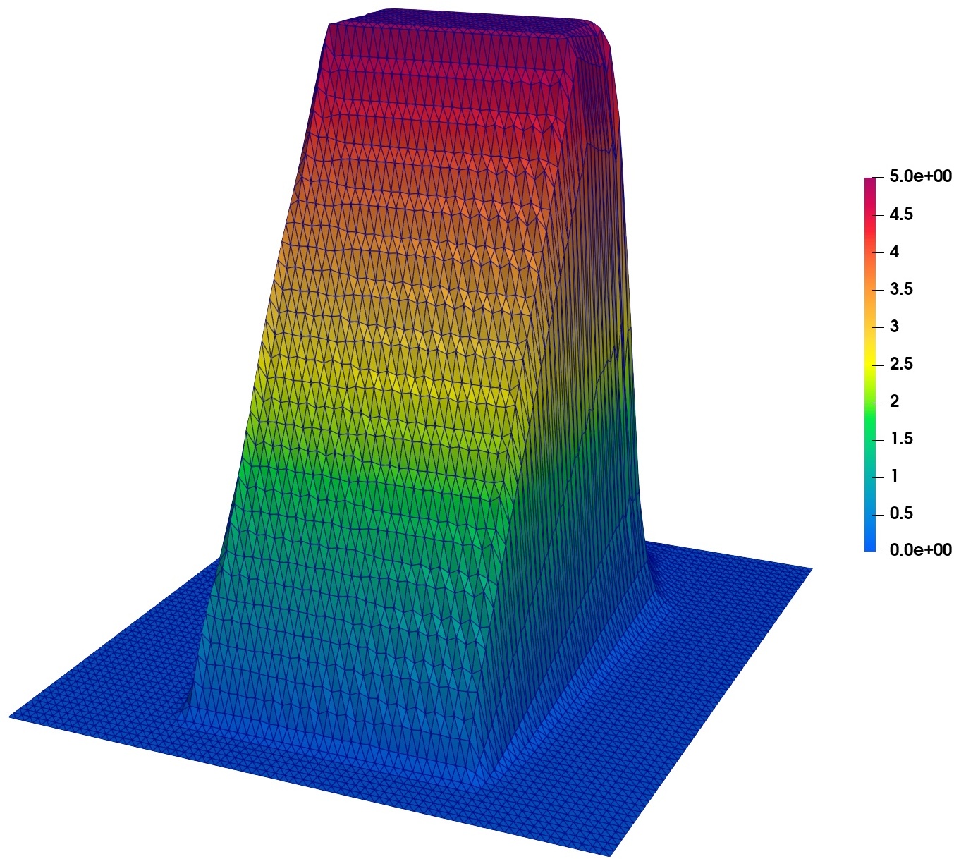
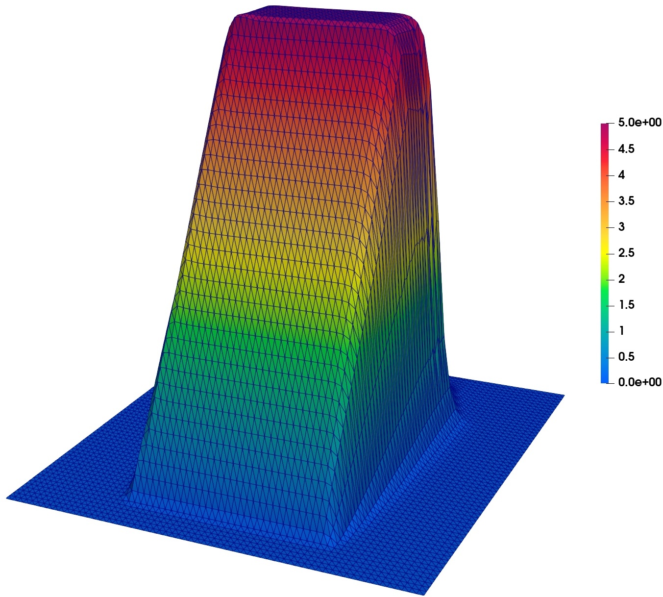
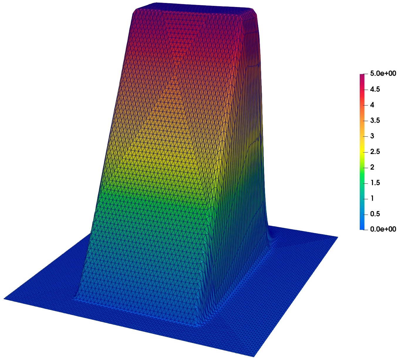
Figure 3: Interior layers, MC (left) and WMC (right) solutions, Grid 1 / level 5.

Figure 4: Interior layers, MC (left) and WMC (right) solutions, Grid 2 / level 5.

The numerical solutions shown in Figs 4 and 4 were obtained on level 5 triangulations of Grid 1 and Grid 2, respectively. The spurious ripples in the MC results are caused by the fact that the flux-corrected approximation to the convective term is not in equilibrium with the standard Galerkin discretization of the source term. The WMC version is free of this drawback and produces nonoscillatory results. Figure 5 shows the Grid 2 / level 7 approximation obtained with WMC.

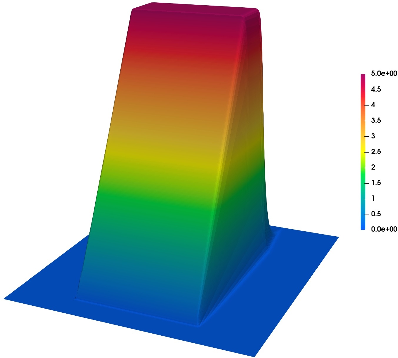
Figure 5: Interior layers, WMC solution, Grid 2 / level 7.

6.2 Boundary layers

The next test problem that we consider in this numerical study was introduced by John et al. in [10, Example 3]. The manufactured exact solution

$$u(x,y)=xy^{2}-y^{2}\exp\left(\frac{2(x-1)}{\varepsilon}\right)-x\exp\left(\frac{3(y-1)}{\varepsilon}\right)+\exp\left(\frac{2(x-1)+3(y-1)}{\varepsilon}\right)$$

of the CDR equation (1a) with $\mathbf{v}=(2,3)^{\top}$ and $c\equiv 0$ is used to define the right-hand side $f$ and the Dirichlet boundary data $u_{D}$. The exact solution has boundary layers at $x=1$ and $y=1$.

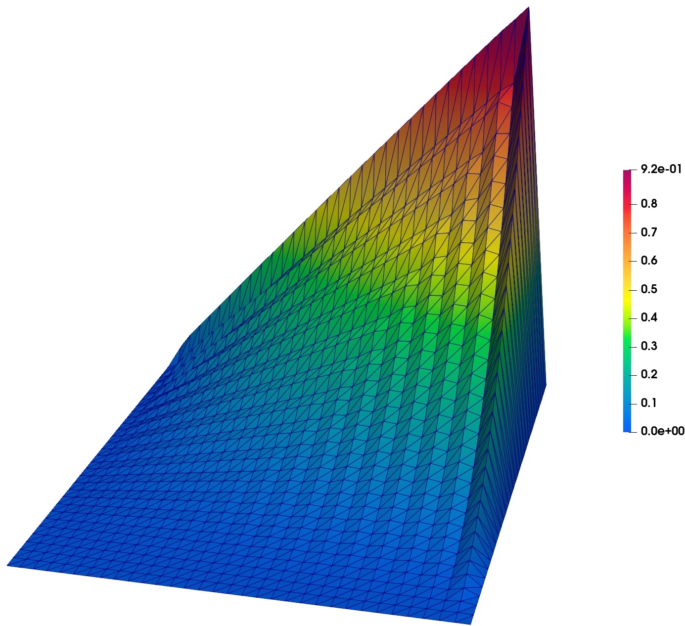
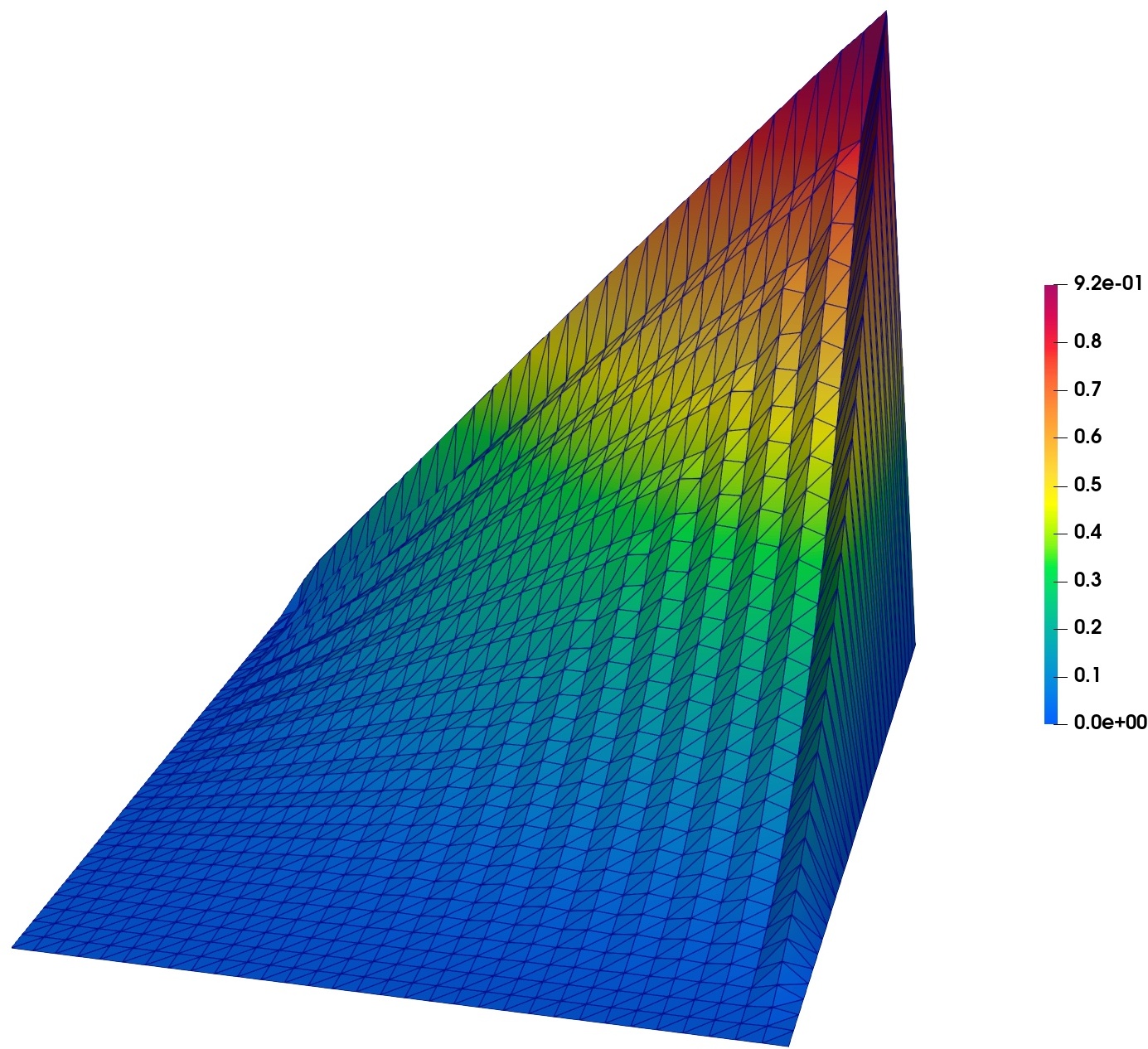
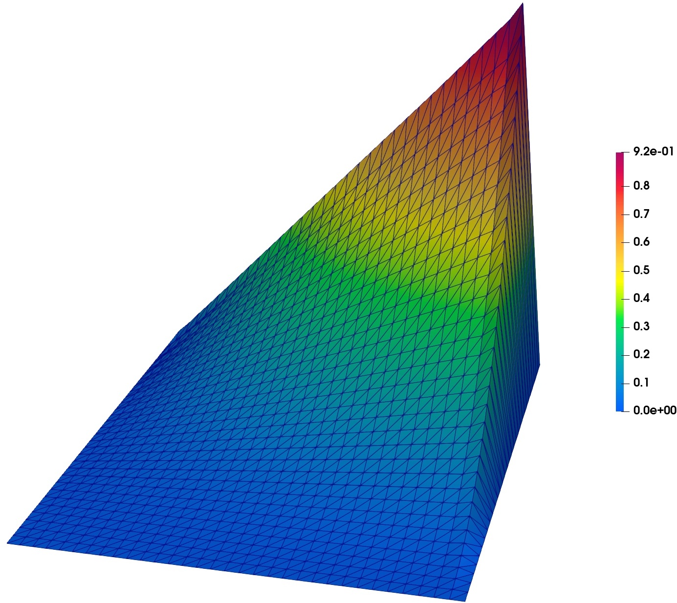
Figure 6: Boundary layers, MC solutions, Grid 1 / level 4, $\varepsilon=10^{-3},10^{-6},$ $10^{-9}$ (left to right).

Figure 7: Boundary layers, WMC solutions, Grid 1 / level 4, $\varepsilon=10^{-3},10^{-6},$ $10^{-9}$ (left to right).

We ran numerical simulations for $\varepsilon\in\left\{10^{-3},10^{-6},10^{-9}\right\}$ on Grid 1 / level 4. The MC and WMC results are presented in Figs 7 and 7, respectively. Once again, the MC version produces spurious oscillations, whereas the WMC approximations are well resolved and free of ripples. Figure 8 shows the WMC result for $\varepsilon=10^{-9}$ obtained using Grid 1 / level 7.

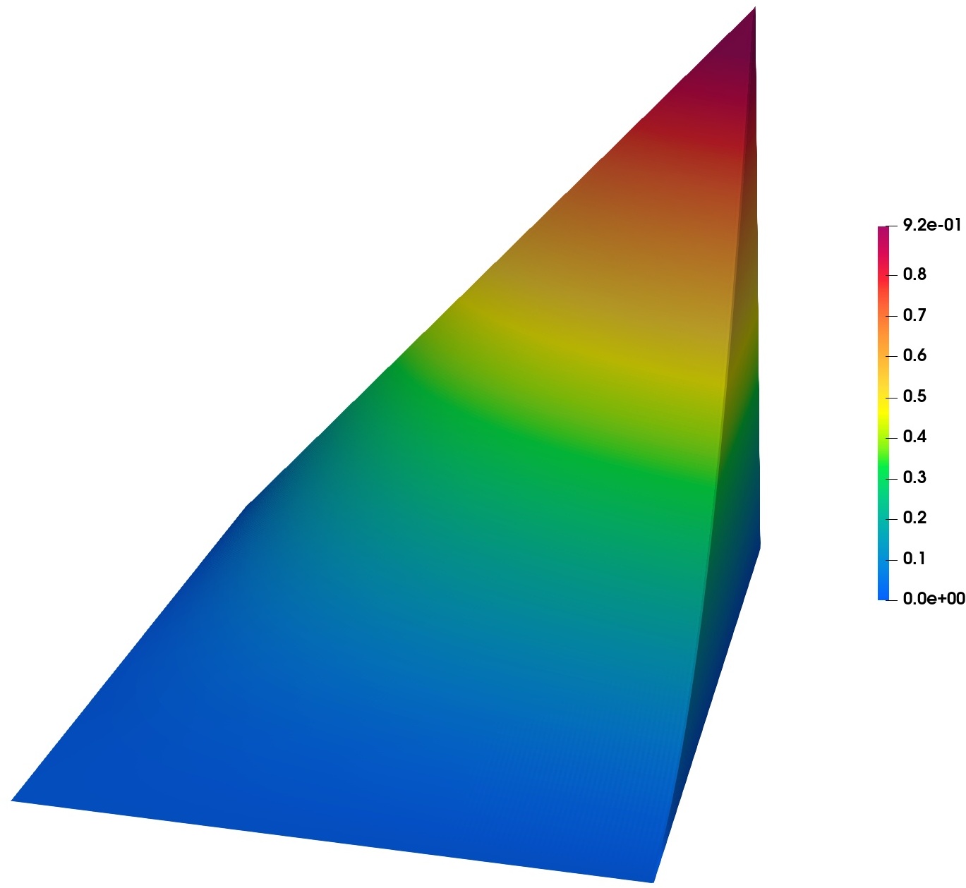
Figure 8: Boundary layers, WMC solution, Grid 1 / level 7, $\varepsilon=10^{-9}$.

6.3 Circular layers

In the next test, we perform numerical experiments for the CDR equation (1a) with the non-constant velocity field $\mathbf{v}=(y,-x)^{\top}$. The source terms are defined by

$$f(x,y)=\left\{\begin{array}[]{ll}1&\mathrm{if}\ \ 0.25\leq\sqrt{x^{2}+y^{2}}\leq 0.75,\\ 0&\mathrm{otherwise},\end{array}\right.$$

and $c(x,y)=1-f(x,y)$. We impose a homogeneous Neumann boundary condition on $\Gamma_{N}=\{(x,0)\,:\,0<x<1\}$ and set $u_{D}=0$ on the Dirichlet boundary $\Gamma_{D}=\Gamma\backslash\Gamma_{N}$.

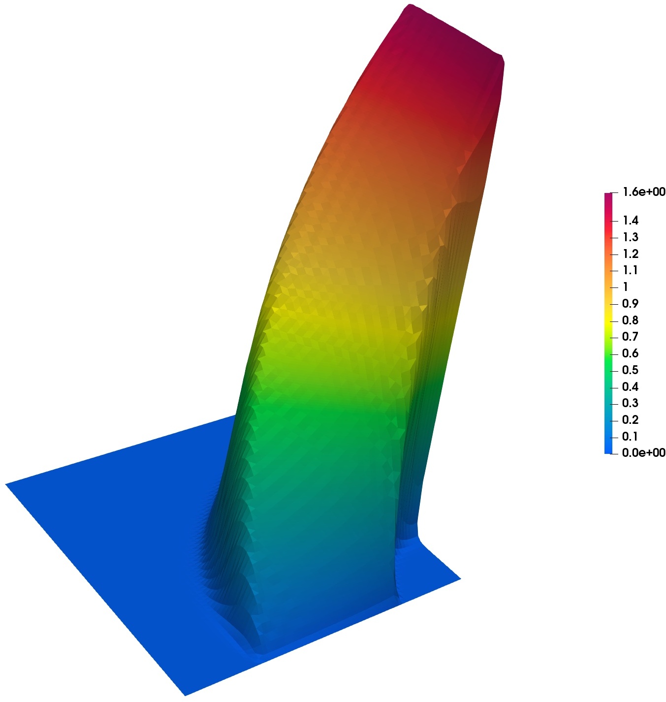
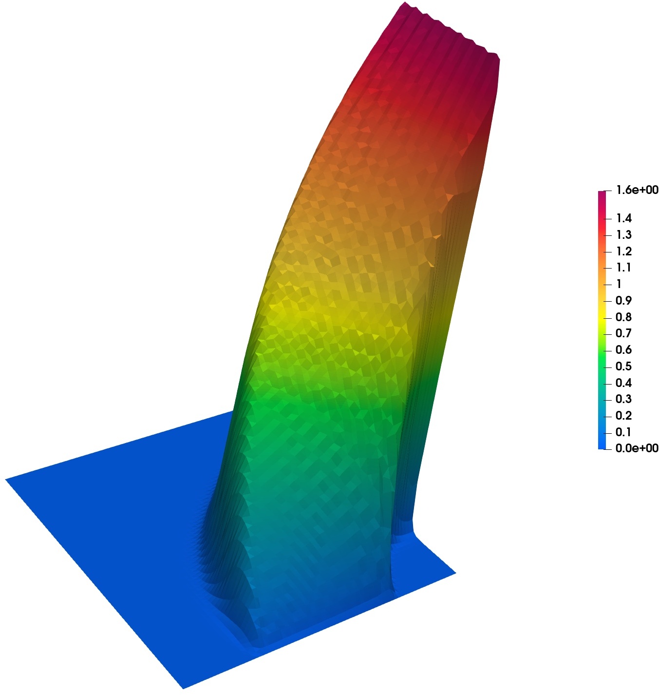
Figure 9: Circular layers, MC solutions, Grid 1 / level 5, $\varepsilon=10^{-4},10^{-6}$ (left to right).

Figure 10: Circular layers, WMC solutions, Grid 1 / level 5, $\varepsilon=10^{-4},10^{-6}$ (left to right).

We ran numerical simulations for $\varepsilon\in\left\{10^{-4},10^{-6}\right\}$ on Grid 1 / level 5. The MC and WMC results are presented in Figs 10 and 10, respectively. Spurious ripples can again be seen in the MC solution of the CDR equation with $\varepsilon=10^{-6}$. Although the exact solution is not linear between the circular internal layers, the WMC approximation is free of ripples. Figure 11 shows the WMC result for $\varepsilon=10^{-4}$ obtained using Grid 1 / level 7.

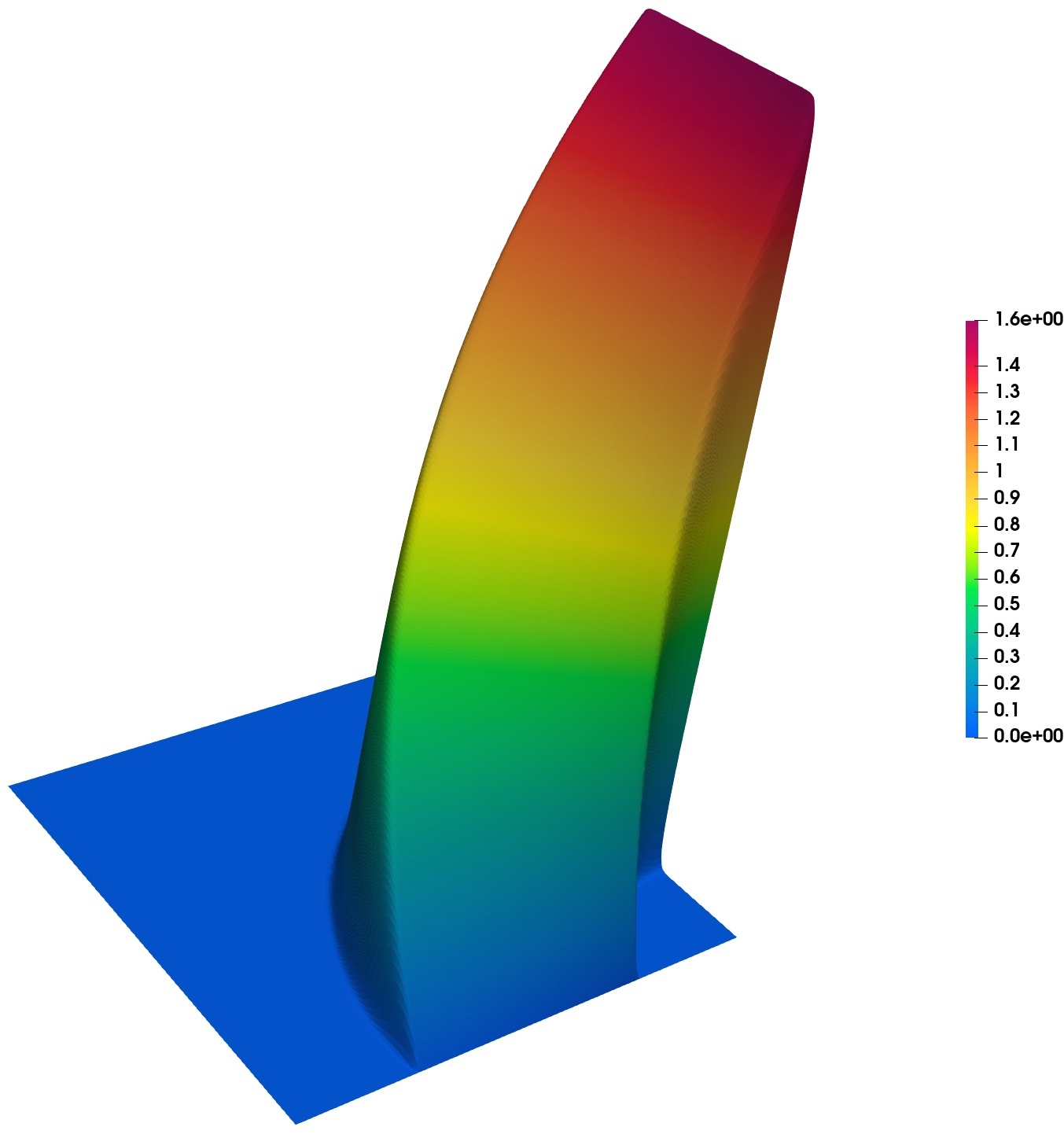
Figure 11: Circular layers, WMC solution, Grid 1 / level 7, $\varepsilon=10^{-4}$.

6.4 Circular convection

In this final example, we study the grid convergence properties of the WMC method. Following Lohmann [15, Eq. (3.24)], we consider equation (1a) with $\varepsilon=0,\mathbf{v}=(y,-x)^{\top}$, and $c\equiv 1$. The smooth exact solution and the inflow boundary condition are given by

$$u(x,y)=\exp\left(-100\left(\sqrt{x^{2}+y^{2}}-0.7\right)^{2}\right),\qquad 0\leq x,y\leq 1.$$

The right-hand side satisfies $f=cu$.

Figure 12 shows the Grid 1 / level 7 solution obtained using the WMC limiter. The experimental order of convergence (E.O.C.) w.r.t. a norm $\|\cdot\|$ is determined using the formula

$$\mathrm{E.O.C.}=\log_{2}\left(\frac{\|u-u_{2h}\|}{\|u-u_{h}\|}\right).$$

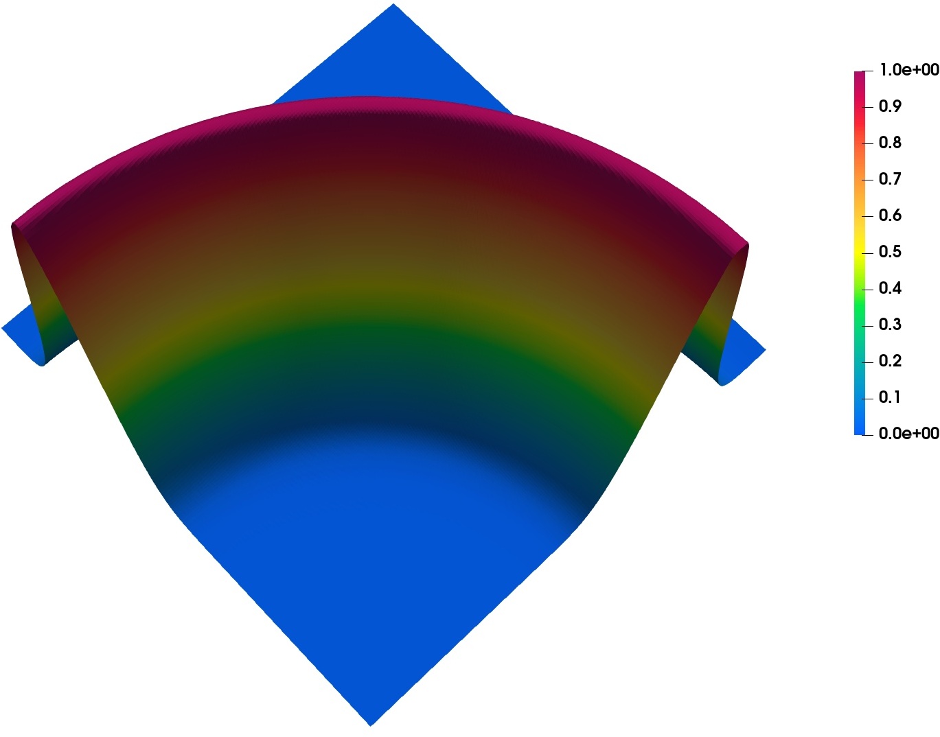
Figure 12: Circular convection, WMC solution, Grid 1 / level 7.

In Tables 1 and 2, we list the $L^{1}$ and $L^{2}$ errors for both types of computational meshes. The Grid 1 and Grid 2 convergence rates approach 2 on fine mesh levels. We conclude that the WMC treatment of source terms does not degrade the convergence behavior of our scheme. Further improvements could be achieved using linearity-preserving local bounds (cf. [12, Example 6.1]).

Level	$\|u-u_{h}\|_{L^{2}}$	E.O.C.	$\|u-u_{h}\|_{L^{1}}$	E.O.C.
3	$0.095\,276\,909\,014\,531$	$0$	$0.057\,723\,388\,291\,951$	$0$
4	$0.038\,372\,306\,081\,693$	$1.312\,061\,139\,879\,611\,6$	$0.018\,893\,367\,506\,366$	$1.611\,276\,119\,755\,095\,5$
5	$0.014\,511\,912\,422\,34$	$1.402\,827\,815\,474\,684$	$0.005\,769\,009\,229\,707\,9$	$1.711\,484\,390\,336\,64$
6	$0.004\,508\,852\,795\,307\,1$	$1.686\,405\,339\,657\,069\,5$	$0.001\,505\,324\,209\,899\,9$	$1.938\,249\,329\,971\,896\,6$
7	$0.001\,272\,604\,191\,414\,9$	$1.824\,976\,631\,411\,569\,6$	$0.000\,329\,000\,365\,774\,43$	$2.193\,913\,148\,537\,673$
8	$0.000\,296\,527\,052\,617\,97$	$2.101\,548\,143\,161\,334$	$0.000\,059\,768\,047\,877\,223$	$2.460\,642\,860\,061\,867$

Table 1: Circular convection, $\|\cdot\|_{L^{2}}$ and $\|\cdot\|_{L^{1}}$ errors for Grid 1 triangulations.

Level	$\|u-u_{h}\|_{L^{2}}$	E.O.C.	$\|u-u_{h}\|_{L^{1}}$	E.O.C.
3	$0.059\,103\,898\,044\,568$	$0$	$0.032\,231\,134\,811\,308$	$0$
4	$0.023\,430\,355\,995\,447$	$1.334\,874\,408\,412\,071$	$0.010\,010\,115\,253\,685$	$1.686\,996\,399\,423\,337$
5	$0.008\,093\,785\,515\,068\,6$	$1.533\,492\,351\,068\,108\,7$	$0.002\,915\,773\,477\,482\,8$	$1.779\,508\,036\,964\,343$
6	$0.002\,476\,325\,884\,763\,6$	$1.708\,613\,432\,289\,037\,8$	$0.000\,758\,337\,010\,149\,84$	$1.942\,967\,603\,431\,133\,4$
7	$0.000\,680\,365\,476\,570\,55$	$1.863\,819\,343\,823\,379\,4$	$0.000\,153\,633\,947\,405\,36$	$2.303\,342\,101\,048\,385$
8	$0.000\,167\,891\,955\,418\,68$	$5.340\,704\,926\,956\,977\,5$	$0.000\,007\,614\,616\,136\,816$	$4.334\,581\,912\,843\,703$

Table 2: Circular convection, $\|\cdot\|_{L^{2}}$ and $\|\cdot\|_{L^{1}}$ errors for Grid 2 triangulations.

7 Conclusions

This paper demonstrates that flux correction tools designed for time-dependent hyperbolic conservation laws require careful adaptation to other types of partial differential equations. In particular, the numerical treatment of source terms becomes important in the steady state limit, which may be affected by algebraic manipulations of the weighted residual formulation. The nonlinear stabilization term of the proposed method includes fluxes that modify the standard Galerkin discretization of source terms in an appropriate manner. The underlying design philosophy is based on an analogy with a well-balanced finite element scheme for the shallow water equations. It is hoped that this analogy (and the way in which it is exploited in the present paper) will advance the development of next-generation flux limiters for finite element discretizations of balance laws.

Acknowledgments

The work of D. Kuzmin was supported by the German Research Foundation (Deutsche Forschungsgemeinschaft, DFG) under grant KU 1530/23-3. The work of P. Knobloch was supported by the grant No. 22-01591S of the Czech Science Foundation.

References

• [1] Paul Arminjon and Alain Dervieux. Construction of TVD-like artificial viscosities on two-dimensional arbitrary FEM grids. J. Comput. Phys., 106(1):176–198, 1993.
• [2] Emmanuel Audusse, Christophe Chalons, and Philippe Ung. A simple well-balanced and positive numerical scheme for the shallow-water system. Communications in Mathematical Sciences, 13(5):1317–1332, 2015.
• [3] Santiago Badia and Jesús Bonilla. Monotonicity-preserving finite element schemes based on differentiable nonlinear stabilization. Comput. Methods Appl. Mech. Engrg., 313:133–158, 2017.
• [4] Gabriel R. Barrenechea, Volker John, and Petr Knobloch. Finite element methods respecting the discrete maximum principle for convection-diffusion equations. SIAM Rev., 66(1), 2024.
• [5] Rosa Donat and Anna Martínez-Gavara. Hybrid second order schemes for scalar balance laws. Journal of Scientific Computing, 48:52–69, 2011.
• [6] Ulrik S. Fjordholm, Siddhartha Mishra, and Eitan Tadmor. Well-balanced and energy stable schemes for the shallow water equations with discontinuous topography. Journal of Computational Physics, 230(14):5587–5609, 2011.
• [7] Llanos Gascón and José Miguel Corberán. Construction of second-order TVD schemes for nonhomogeneous hyperbolic conservation laws. Journal of Computational Physics, 172(1):261–297, 2001.
• [8] Hennes Hajduk. Algebraically Constrained Finite Element Methods for Hyperbolic Problems With Applications to Geophysics and Gas Dynamics. PhD thesis, TU Dortmund University, 2022.
• [9] Hennes Hajduk and Dmitri Kuzmin. Bound-preserving and entropy-stable algebraic flux correction schemes for the shallow water equations with topography. Technical report, arXiv:2207.07261 [math.NA], 2022.
• [10] Volker John, Joseph M. Maubach, and Lutz Tobiska. Nonconforming streamline-diffusion-finite-element-methods for convection-diffusion problems. Numerische Mathematik, 78(2):165–188, December 1997.
• [11] Petr Knobloch. An algebraically stabilized method for convection-diffusion-reaction problems with optimal experimental convergence rates on general meshes. Numer. Algorithms, 94(2):547–580, 2023.
• [12] Dmitri Kuzmin. Monolithic convex limiting for continuous finite element discretizations of hyperbolic conservation laws. Computer Methods in Applied Mechanics and Engineering, 361:112804, 2020.
• [13] Dmitri Kuzmin and Hennes Hajduk. Property-Preserving Numerical Schemes for Conservation Laws. World Scientific, 2023.
• [14] Randall J. LeVeque. Balancing source terms and flux gradients in high-resolution Godunov methods: The quasi-steady wave-propagation algorithm. Journal of Computational Physics, 146(1):346–365, 1998.
• [15] Christoph Lohmann. Physics-Compatible Finite Element Methods for Scalar and Tensorial Advection Problems. Springer, 2019.
• [16] Paulo R. M. Lyra, Kenneth Morgan, Jaime Peraire, and Joaquim Peiró. TVD algorithms for the solution of the compressible Euler equations on unstructured meshes. Internat. J. Numer. Methods Fluids, 19(9):827–847, 1994.
• [17] Sebastian Noelle, Normann Pankratz, Gabriella Puppo, and Jostein R Natvig. Well-balanced finite volume schemes of arbitrary order of accuracy for shallow water flows. Journal of Computational Physics, 213(2):474–499, 2006.
• [18] Hans-Görg Roos, Martin Stynes, and Lutz Tobiska. Robust Numerical Methods for Singularly Perturbed Differential Equations, volume 24 of Springer Series in Computational Mathematics. Springer-Verlag, Berlin, second edition, 2008.
• [19] Peter K. Sweby. "TVD" schemes for inhomogeneous conservation laws. In Josef Ballmann and Rolf Jeltsch, editors, Nonlinear Hyperbolic Equations—Theory, Computation Methods, and Applications: Proceedings of the Second International Conference on Nonlinear Hyperbolic Problems, Aachen, FRG, March 14 to 18, 1988, pages 599–607. Springer, 1989.
• [20] Roger Temam. Navier-Stokes equations. Theory and numerical analysis. North-Holland Publishing Co., Amsterdam-New York-Oxford, 1977. Studies in Mathematics and its Applications, Vol. 2.
• [21] Ulrich Wilbrandt, Clemens Bartsch, Naveed Ahmed, Najib Alia, Felix Anker, Laura Blank, Alfonso Caiazzo, Sashikumaar Ganesan, Swetlana Giere, Gunar Matthies, Raviteja Meesala, Abdus Shamim, Jagannath Venkatesan, and Volker John. ParMooN – A modernized program package based on mapped finite elements. Computers and Mathematics with Applications, 74:74–88, 2016.