Comparing Data-Driven and Mechanistic Models for Predicting Phenology in Deciduous Broadleaf Forests

Abstract

Understanding the future climate is crucial for informed policy decisions on climate change prevention and mitigation. Earth system models play an important role in predicting future climate, requiring accurate representation of complex sub-processes that span multiple time scales and spatial scales. One such process that links seasonal and interannual climate variability to cyclical biological events is tree phenology in deciduous broadleaf forests. Phenological dates, such as the start and end of the growing season, are critical for understanding the exchange of carbon and water between the biosphere and the atmosphere. Mechanistic prediction of these dates is challenging. Hybrid modelling, which integrates data-driven approaches into complex models, offers a solution. In this work, as a first step towards this goal, train a deep neural network to predict a phenological index from meteorological time series. We find that this approach outperforms traditional process-based models. This highlights the potential of data-driven methods to improve climate predictions. We also analyze which variables and aspects of the time series influence the predicted onset of the season, in order to gain a better understanding of the advantages and limitations of our model.

1 Introduction

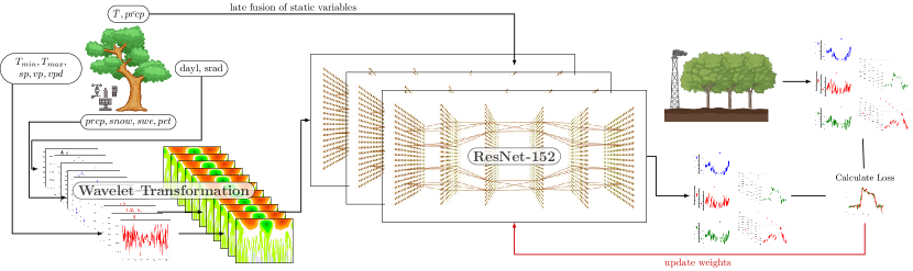
Figure 1: Our approach to predicting the green chromatic coordinate from meteorological variables. We use a wavelet transform on meteorological data from the current and previous years and an ensemble of ResNets to predict phenology and several auxiliary labels.

Understanding the future climate is important towards making political decisions for climate change prevention and mitigation. The main method to predict future climate are large Earth’s system models (ESMs). These models need to represent many complex sub-processes that span multiple time scales and spacial scales to make good predictions. One such process is tree phenology in deciduous broadleaf forest. Phenology describes the timing of periodic events in biological life cycles and links them to seasonal and interannual variations in climate[12], for example the date when trees start to grow or shed their leafs. Since understanding the length of the season in which the trees carry functional leafs is essential to understand the exchange of carbon and water between the biosphere and the atmosphere [28], in this work, we aim to predict the stat of this season (SoS) and end of this season (EoS).

Two challenges emerge when predicting these phenological dates. First, the change between dormancy and maximum leafs is not instantaneous but the number and maturity of leaves increases gradually. Hence, researchers have to rely on thresholds. However, previous work demonstrated that the choice of threshold has a significant influence on interannual patterns and long-term trends of these dates [14]. Second, the processes that relate meteorological events to these dates are non-linear, complex and not fully understood. Nevertheless, ESMs often rely on simple models that use only very few simple meteorological features, for example [16], or even prescribed phenology, for example [1, 22, 31].

One approach that can aid in addressing these challenges is hybrid modeling, as suggested by [15] and applied in similar situations, for example, by [3, 5]. Hybrid modeling is an approach where, in a complex model, some parts are replaced by data-driven models. For phenology, large datasets are available from satellite observations [26], in-situ studies [11], and near-remote sensing [28, 23]. In this work, we present a data-driven model for phenology. This is a first step towards replacing the phenology model in a land surface model (LSM). We train a convolutional neural network (CNN), namely a ResNet-152[7], on near-remote sensing observations of a plant phenological index in deciduous broadleaf forest.

Near-remote sensing data is available in higher temporal resolutions and is more objective than in-situ observations [11]. Further, they are less susceptible to atmospheric disturbance like clouds than satellite observations [19]. To tackle the challenges mentioned above, we, first, not only predict the phenological dates SoS and EoS, but daily greenness indices, allowing us to calculate the dates with different thresholds post-hoc. Second, we use a ResNet, which can learn complex relations between meteorological time series and the phenological index from the data.

We compare our data-driven approach to two process-based approaches. First, LoGrop-P, the phenology model of JSBACH [16], the LSM of ICON-ESM [10]; and second, a model that prescribes phenology. We find that the data-driven model reduces the error compared to these models for daily greenness by 16% and for the start of season (SoS) by 47% / 9%. However, we find no improvement in predicting the end of season (EoS) and, in an ablation study, we find that our approach is only slightly better than simpler data-driven models.

Finally, we use two methods to interpret the neural network. First, we use Integrated Gradients (IG) [24] to understand which variables have the largest influence towards the start of season. To understand, in particular, which time scales are important, we perform a wavelet transformation (WT) on the input time series before using the CNN. We find that the network relies primarily on features and scales that are more informative of the general climate than meteorological events.

Secondly, we employ an approach based on causal inference [18] to validate that the CNN relies on growing degree days (GDD) and chilling days two higher level descriptors of the temperature time-series that are known to be important towards the SoS and are used by the LoGro-P model.

2 Related Work

Predicting the greenness of forests using machine learning has been attempted before. For example, [27] conducted a challenge where teams predicted the greenness of multiple different sites up to 30 days ahead. In contrast to this work, where we train one global model, the teams in the challenge trained one model per site. Further, they did not use deep learning, but mostly simpler data-driven approaches. In contrast, [6] trained a Long Short Term Memory model but also only on a single site in the US.

3 Data and Methods

To calculate the phenological state of the forest, we use the green chromatic coordinate (GCC) [19] from observations provided by the PhenoCam network [23]. Digital images are captured at various locations throughout North America at intervals ranging from half-hourly to daily. For each site, a region of interest containing the canopy is selected, and the mean RGB color is calculated. The GCC is given by

$$GCC=G/(R+G+B).$$ (1)

Following previous work [28], we use the 90^th percentile of GCC for each day as the target. The GCC dataset we use is provided by the PhenoCam network [23]. We use the data from all deciduous broadleaf forest sites in the network that, contain at least one year of observations, are in the top two data-quality groups and contain no GCC value below 0.1 or above 0.6. The data is standardized such that the smallest value becomes zero and the largest value becomes one. We split the sites randomly into 66 sites for training (247 site years), 9 sites for validation (37 site years), and 16 sites for testing (73 site years).

As input, we use eleven meteorological variables: day length, precipitation, short-wave radiation, snow-water equivalent, vapor pressure, vapor pressure deficit (VPD), minimum and maximum air temperature (T_min, T_max), potential evapotranspiration, snow, and surface air pressure. The first ten variables are part of Daymet project[25], a project that interpolates meteorological variables from ground-based measurements, and the air pressure is taken from ERA-5 [8] reanalysis data.

Following [30], we decided for a direct rather than iterative multi-step prediction. We predict the 365 yearly values of GCC simultaneously using one neural network with 365 outputs. Further, to account for legacy effects in vegetation, for example, reported in [29], we use the meteorological observations of the current and the previous year, leaving us with eleven time series of 730 days. We use a continuous wavelet transformation on each of the time series individually. We use the Ricker-wavelet [20] with a scale of $2^{i}$ days for $i\in\{-1,\dots,8\}$ positioned at each day of the time series using zero padding.

We train a ResNet [7] on the wavelet-transformed time series. We stack the results for the ten scales for all eleven variables along the first axis to create a 108 by 730 input with one channel. All input values are normalized to mean zero and standard deviation one. Further, we use a late fusion of the annual temperature and precipitation means over 30 years after the convolutional part of the ResNet. We pre-train on ImageNet [21] and afterwards alter the CNN to the suitable input and output dimensions.

Using [2], we optimize the size of the ResNet ({18, 34, 50, 101, 152}; optimal: 152) along other hyper-parameters on the validation set. The other hyper-parameters are batch size ([1, 128]; optimal: 1), learning rate ([0.00001, 1]; optimal: 0.912), the parameters of the cosine annealing with warm restarts ($t_{0}$: [10, 1000]; optimal: 790), the optimizer used ({Adam, SGD}; optimal: SGD), and the number of epochs before training stops early ([1, 100]; optimal: 18).

To avoid over-fitting, we use multiple auxiliary tasks. In addition to the 90^th GCC percentile, we predict 20 additional color indices provided by the PhenoCam network, as well as five yearly values for kernel-NDVI [26] from MODIS [13]: mean, standard deviation, and 50^th, 75^th, and 90^th percentile. We standardize all labels and minimize the sum over the individual mean squared errors. To focus on GCC, we multiply the loss of the auxiliary tasks with a constant $0<\lambda<1$, which we optimized as an additional hyper-parameter on the validation set ([0,1]; optimal: 0.890). An overview is displayed in Figure 1. Finally, we add a random walk as an additional input. Later, we want to interpret the importance of each variable, time-point, and scale using IG. To this end, we dismiss any value that is less important than the 99.9 percentile of the random walk’s importance scores.

To reach a better generalization performance, we train twenty of these neural networks and use them in an ensemble for inference. To this end, we calculate the final prediction as a weighted mean over the predictions of the individual models. The weights are optimized using the validation set.

Additionally, we want to understand whether our data-driven model relies on high level features of the temperature time-series. Since these features are not input variables, we cannot use IG or comparable methods to determine whether they are relevant to the decision of the neural network. Instead we use [18], a method based on causal inference. This method reduces the question whether a feature is used by a deep neural network to a conditional dependence test. We use the HSConIC [4] for this conditional dependence test with a level of significance of $p=0.05$. Following [17], we validate that this method is suitable, by adding two features that do not influence the SoS but are of similar complexity to the features of interest.

4 Experiments and Results

To understand the quality and limitations of our data-driven model, we conduct four experiments: First, we evaluate our model against two mechanistic models; second, we conduct an ablation study on the different parts of our model; third, we quantify the importance of each variable towards the SoS; and finally, we evaluate whether the network uses the same features as mechanistic models.

We compare the data-driven model (last line of Table 1) to two mechanistic models. The first model uses a prescribed phenology (first line of Table 1). For this model we prescribe $\mathbb{E}(GCC\,|\,DoY)$ the average GCC per day of year on the training set. The second model is LoGro-P, the phenology model of JSBACH [16] (second line of Table 1).

For these models we compare the coefficient of determination between predictions and observations for GCC (R²), on the GCC anomalies (R${}^{2}_{\textup{anomalies}}$), on the start of season (SoS R²), and end of season (EoS R²). Additionally, we report the root mean squared error for the GCC values (RMSE), the SoS (SoS RMSE), and the EoS (EoS RMSE).

To estimate the start and end of season, we use the halfway point between the highest and lowest GCC as a threshold. The LoGro-P model predicts the leaf area index instead of GCC but it is highly related to GCC [28]. For this reason and because of the difficulties mentioned in [14], we calibrate the estimations of the SoS and EoS of each model by training a linear correction on the validation set.

The results of the comparison are presented in Table 1. The data-driven approach outperforms the mechanistic models for GCC and SoS, but not for EoS. The model increases R² by $13\%$ and reduces the RMSE by $16\%$ compared to prescribing phenology. For the SoS, the model reduces the RMSE by $47\%$ (7.0 days) compared to the prescribed phenology and by $9\%$ (0.9 days) compared to LoGro-P. However, the coefficient of determination on the anomalies is only $0.198$, and, for EoS, the error increased by $3\%$ (1.2 days).

In the ablation study, we remove the wavelet transformation and/or replace the ResNet by linear regression. We find that the simpler models have a similar performance. The $R^{2}$ of the full model is identical to the linear regression and the SoS RSME of the linear regression is 3.7% higher than for the full model. Only R${}^{2}_{\textup{anomalies}}$ improved notably ($27\%$).

Table 1: The performance on the twelve holdout test sets. The best value in each column is bold

Model	R2	R${}^{2}_{\textup{anomalies}}$	RMSE	SoS R2	SoS RMSE	EoS R2	EoS RMSE
Prescribed Phenology	0.599	0.000	0.031	0.000	14.9	0.000	34.9
LoGro-P[16]	–	–	–	0.688	8.7	-0.010	34.9
Linear Regression	0.661	0.155	0.026	0.697	8.2	-0.056	35.2
+ Wavelet	0.630	0.078	0.028	0.632	9.0	-0.024	35.8
ResNet	0.643	0.112	0.028	0.716	7.9	-0.094	37.0
+ Wavelet	0.678	0.198	0.026	0.720	7.9	-0.025	36.1

Third, we want to quantify the importance of each variable towards the prediction of SoS by IG [24]. However, the SoS is not directly the output of the neural network. To be able to use IG, we add an additional layer to the CNN, calculating

$$150-\sum_{t=80}^{150}\sigma(\textup{gcc}_{t}-0.5)$$ (2)

with $\sigma$ the sigmoid function. The result of this calculation is virtually identical to the values determined by the threshold method ($R^{2}=0.986$). For the importance analysis, we exclude years where the start of season is predicted before day 80. The results are displayed in Figure 3. The most important variables are the snow, the potential evapotranspiration, which is a predictor of the soil moisture, and the minimum temperature. While these features are known to be meaningful towards the SoS, we find that all days are of similar importance and long, close to yearly, periods are much more relevant than daily periods, indicating that the network relies on a general climate rather than specific meteorological events.

We compare this result, to the coefficients of the linear classifier. Following [9] we multiply each linear coefficient with the standard deviation of the variable. We consider the linear classifier for day of year (DoY) 120. Similar to our model, the linear classifier also relies on all days and not specifically on the DoYs directly prior to DoY 120. Further, the three most importance features according to the linear classifier are the air pressure, the vapor pressure and the vapor pressure deficit. The minimum temperature, a feature that many mechanistic models use exclusively, is ranked eighths.

Figure 2: The observation and prediction for one example from the test set.

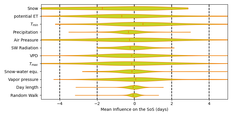
Figure 3: The importance of each variable as evaluated by IG. The variables are ordered by absolute mean importance. Each row shows the distribution of influences on the SoS over all site-years. The orange line marks the mean.

Finally we want to test whether our model relies on the same high-level features as the mechanistic LoGro-P model. This model relies on two features to predict the SoS [16]: the chill days, the number of days below four degrees Celsius before a day of the year, and the growing degree days

$$GDD=\sum_{t=1}^{doy}\max(0,T_{t}-277.15\textup{K})$$ (3)

where $T_{t}$ is the mean temperature at day $t$. We determine whether our model also relies on these features at DoY 120. To avoid detecting the importance of the average temperature, we decorrelate these features from from the average temperature. Following [17], we validate that this method of [18] is suitable, by testing two additional features that do not influence the SoS but are of similar complexity to the features of interest: the chill days and GDD of the previous year.

We find that the network uses the chill days and growing degree days of the current but not the previous year to determine the SoS.

5 Conclusions and Future Research

In this work we compare a data-driven method to two mechanistic models. We find that our model performs better in predicting the greenness of canopies and in predicting the start of season. However, the architecture only slightly outperforms much simpler architectures. We further analysed which features are used by the neural network to predict the start of season. While we found that our model considers the features used by the mechanistic LoGro-P model and considers variables relevant that are considered by experts, the analysis with integrated gradients revealed that the model considers mainly long time scales and does not focus on the time period directly before the start of season. This indicates that the model understood the impact of the brought climate on the phenology but not the influence of meteorological events.

We found that no model can detect the end of season with any accuracy. This might be due to problems in the data that might already add a high amount of uncertainty to the day of year when the end of season is observed. Further, the data has considerable differences between sites, likely due to differences in the data acquisition, for example, different orientations and angles of the cameras.

Therefore, this approach could be improved by considering data from different sources or putting a stronger focus on normalizing the GCC data according to site specific properties.

References

- [1] IT Baker, L Prihodko, AS Denning, Michael Goulden, S Miller, and HR Da Rocha. Seasonal drought stress in the amazon: Reconciling models and observations. Journal of Geophysical Research: Biogeosciences, 113(G1), 2008.
- [2] James Bergstra, Rémi Bardenet, Yoshua Bengio, and Balázs Kégl. Algorithms for hyper-parameter optimization. Advances in neural information processing systems, 24, 2011.
- [3] RedaReda ElGhawi, Basil Kraft, Christian Reimers, Markus Reichstein, Marco Körner, Pierre Gentine, and Alexander J WinklerWinkler. Hybrid modeling of evapotranspiration: inferring stomatal and aerodynamic resistances using combined physics-based and machine learning. Environmental Research Letters, 18(3):034039, 2023.
- [4] Kenji Fukumizu, Arthur Gretton, Xiaohai Sun, and Bernhard Schölkopf. Kernel measures of conditional dependence. Advances in neural information processing systems, 20, 2007.
- [5] Arthur Grundner, Tom Beucler, Pierre Gentine, Fernando Iglesias-Suarez, Marco A Giorgetta, and Veronika Eyring. Deep learning based cloud cover parameterization for icon. Journal of Advances in Modeling Earth Systems, 14(12):e2021MS002959, 2022.
- [6] Peng Guan, Yili Zheng, and Guannan Lei. Analysis of canopy phenology in man-made forests using near-earth remote sensing. Plant Methods, 17(1):1–15, 2021.
- [7] Kaiming He, Xiangyu Zhang, Shaoqing Ren, and Jian Sun. Deep residual learning for image recognition. In Proceedings of the IEEE conference on computer vision and pattern recognition, pages 770–778, 2016.
- [8] Hans Hersbach, Bill Bell, Paul Berrisford, Shoji Hirahara, András Horányi, Joaquín Muñoz-Sabater, Julien Nicolas, Carole Peubey, Raluca Radu, Dinand Schepers, et al. The era5 global reanalysis. Quarterly Journal of the Royal Meteorological Society, 146(730):1999–2049, 2020.
- [9] Martin Jung, Markus Reichstein, Christopher R Schwalm, Chris Huntingford, Stephen Sitch, Anders Ahlström, Almut Arneth, Gustau Camps-Valls, Philippe Ciais, Pierre Friedlingstein, et al. Compensatory water effects link yearly global land co2 sink changes to temperature. Nature, 541(7638):516–520, 2017.
- [10] Johann H Jungclaus, Stephan J Lorenz, Hauke Schmidt, Victor Brovkin, Nils Brüggemann, Fatemeh Chegini, Traute Crüger, Philipp De-Vrese, Veronika Gayler, Marco A Giorgetta, et al. The icon earth system model version 1.0. Journal of Advances in Modeling Earth Systems, 14(4):e2021MS002813, 2022.
- [11] Guohua Liu, Isabelle Chuine, Rémy Denéchère, Frédéric Jean, Eric Dufrêne, Gaëlle Vincent, Daniel Berveiller, and Nicolas Delpierre. Higher sample sizes and observer inter-calibration are needed for reliable scoring of leaf phenology in trees. Journal of Ecology, 109(6):2461–2474, 2021.
- [12] Merriam-Webster. Phenology.
- [13] ORNL DAAC. Modis and viirs land products global subsetting and visualization tool, 2018.
- [14] Annu Panwar, Mirco Migliavacca, Jacob A Nelson, José Cortés, Ana Bastos, Matthias Forkel, and Alexander J Winkler. Methodological challenges and new perspectives of shifting vegetation phenology in eddy covariance data. Scientific Reports, 13(1):13885, 2023.
- [15] Markus Reichstein, Gustau Camps-Valls, Bjorn Stevens, Martin Jung, Joachim Denzler, Nuno Carvalhais, and fnm Prabhat. Deep learning and process understanding for data-driven earth system science. Nature, 566(7743):195–204, 2019.
- [16] Christian H Reick, Veronika Gayler, Daniel Goll, Stefan Hagemann, Marvin Heidkamp, Julia EMS Nabel, Thomas Raddatz, Erich Roeckner, Reiner Schnur, and Stiig Wilkenskjeld. Jsbach 3-the land component of the mpi earth system model: documentation of version 3.2. 2021.
- [17] Christian Reimers, Niklas Penzel, Paul Bodesheim, Jakob Runge, and Joachim Denzler. Conditional dependence tests reveal the usage of abcd rule features and bias variables in automatic skin lesion classification. In Proceedings of the IEEE/CVF Conference on Computer Vision and Pattern Recognition, pages 1810–1819, 2021.
- [18] Christian Reimers, Jakob Runge, and Joachim Denzler. Determining the relevance of features for deep neural networks. In European Conference on Computer Vision, pages 330–346. Springer, 2020.
- [19] Andrew D Richardson, Julian P Jenkins, Bobby H Braswell, David Y Hollinger, Scott V Ollinger, and Marie-Louise Smith. Use of digital webcam images to track spring green-up in a deciduous broadleaf forest. Oecologia, 152:323–334, 2007.
- [20] Norman Ricker. Further developments in the wavelet theory of seismogram structure. Bulletin of the Seismological Society of America, 33(3):197–228, 1943.
- [21] Olga Russakovsky, Jia Deng, Hao Su, Jonathan Krause, Sanjeev Satheesh, Sean Ma, Zhiheng Huang, Andrej Karpathy, Aditya Khosla, Michael Bernstein, et al. Imagenet large scale visual recognition challenge. International journal of computer vision, 115:211–252, 2015.
- [22] Kevin Schaefer, G James Collatz, Pieter Tans, A Scott Denning, Ian Baker, Joe Berry, Lara Prihodko, Neil Suits, and Andrew Philpott. Combined simple biosphere/carnegie-ames-stanford approach terrestrial carbon cycle model. Journal of Geophysical Research: Biogeosciences, 113(G3), 2008.
- [23] B. Seyednasrollah, A.M. Young, K. Hufkens, T. Milliman, M.A. Friedl, S. Frolking, M. Richardson, A.D. a nd Abraha, D.W. Allen, M. Apple, M.A. Arain, J. Baker, J.M. Baker, D. Baldocchi, C.J. Bernacchi, J. Bhat tacharjee, P. Blanken, D.D. Bosch, R. Boughton, E.H. Boughton, R.F. Brown, D.M. Browning, S.P. Brunsell, N. an d Burns, M. Cavagna, H. Chu, P.E. Clark, B.J. Conrad, E. Cremonese, D. Debinski, A.R. Desai, R. Diaz-D elgado, L. Duchesne, A.L. Dunn, D.M. Eissenstat, T. El-Madany, D.S.S. Ellum, S.M. Ernest, L. Esposito, A. an d Fenstermaker, L.B. Flanagan, B. Forsythe, J. Gallagher, D. Gianelle, T. Griffis, P. Groffman, J. Gu, L. an d Guillemot, M. Halpin, P.J. Hanson, D. Hemming, A.A. Hove, E.R. Humphreys, A. Jaimes-Hernandez, A.A. Jaradat, J. Johnson, E. Keel, V.R. Kelly, J.W. Kirchner, P.B. Kirchner, M. Knapp, M. Krassovski, O. Langvall, G. Lanthier, G.l. Maire, E. Magliulo, T.A. Martin, B. McNeil, G.A. Meyer, M. Migliavacca, B. P. Mohanty, C.E. Moore, R. Mudd, J.W. Munger, Z.E. Murrell, Z. Nesic, H.S. Neufeld, T.L. O’Halloran, A.C. Oechel, W. a nd Oishi, W.W. Oswald, T.D. Perkins, M.L. Reba, B. Rundquist, B.R. Runkle, E.S. Russell, A. Sadler, E.J. a nd Saha, N.Z. Saliendra, L. Schmalbeck, M.D. Schwartz, R.L. Scott, E.M. Smith, O. Sonnentag, P. Stoy, S. Strachan, K. Suvocarev, J.E. Thom, R.Q. Thomas, A.K. Van den berg, R. Vargas, J. Verfaillie, C.S. Vogel, J.J. Walker, N. Webb, P. Wetzel, S. Weyers, A.V. Whipple, T.G. Whitham, G. Wohlfahrt, J.D. Wood, S. Wo lf, J. Yang, X. Yang, G. Yenni, Y. Zhang, Q. Zhang, and D. Zona. Phenocam dataset v2.0: Vegetation phenology from digital camera imagery, 2000-2018. 2019.
- [24] Mukund Sundararajan, Ankur Taly, and Qiqi Yan. Axiomatic attribution for deep networks. In International conference on machine learning, pages 3319–3328. PMLR, 2017.
- [25] MM Thornton, R Shrestha, Y Wei, PE Thornton, SC Kao, BE Wilson, BW Mayer, Y Wei, R Devarakonda, RS Vose, et al. Daymet: daily surface weather data on a 1-km grid for north america, version 4 r1. ORNL DAAC, Oak Ridge, Tennessee, USA. Single Pixel Extraction Tool| Daymet (ornl. gov), 2022.
- [26] Qiang Wang, Álvaro Moreno-Martínez, Jordi Muñoz-Marí, Manuel Campos-Taberner, and Gustau Camps-Valls. Estimation of vegetation traits with kernel ndvi. ISPRS Journal of Photogrammetry and Remote Sensing, 195:408–417, 2023.
- [27] Kathryn Wheeler, Michael Dietze, David LeBauer, Jody Peters, Andrew D. Richardson, R. Quinn Thomas, Kai Zhu, Uttam Bhat, Stephan Munch, Raphaela Floreani Buzbee, Min Chen, Benjamin Goldstein, Jessica S. Guo, Dalei Hao, Chris Jones, Mira Kelly-Fair, Haoran Liu, Charlotte Malmborg, Naresh Neupane, Debasmita Pal, Arun Ross, Vaughn Shirey, Yiluan Song, McKalee Steen, Eric A. Vance, Whitney M. Woelmer, Jacob Wynne, and Luke Zachmann. Predicting spring phenology in deciduous broadleaf forests: An open community forecast challenge. SSRN Electronic Journal, 2023.
- [28] Lisa Wingate, Jérôme Ogée, Edoardo Cremonese, Gianluca Filippa, Toshie Mizunuma, Mirco Migliavacca, Christophe Moisy, Matthew Wilkinson, Christine Moureaux, Georg Wohlfahrt, et al. Interpreting canopy development and physiology using a european phenology camera network at flux sites. Biogeosciences, 12(20):5995–6015, 2015.
- [29] Xin Yu, René Orth, Markus Reichstein, Michael Bahn, Anne Klosterhalfen, Alexander Knohl, Franziska Koebsch, Mirco Migliavacca, Martina Mund, Jacob A Nelson, et al. Contrasting drought legacy effects on gross primary productivity in a mixed versus pure beech forest. Biogeosciences, 19(17):4315–4329, 2022.
- [30] Ailing Zeng, Muxi Chen, Lei Zhang, and Qiang Xu. Are transformers effective for time series forecasting? In Proceedings of the AAAI conference on artificial intelligence, volume 37, pages 11121–11128, 2023.
- [31] Xiwu Zhan, Yongkang Xue, and G James Collatz. An analytical approach for estimating co2 and heat fluxes over the amazonian region. Ecological Modelling, 162(1-2):97–117, 2003.