Breathing mode of a quantum droplet in a quasi-one-dimensional dipolar Bose gas

Abstract

We investigate the breathing mode and the stability of a quantum droplet in a tightly trapped one-dimensional dipolar gas of bosonic atoms. When the droplet with a flat-top density profile is formed, the breathing mode frequency scales as the inverse of the number of atoms in the cloud. This is straightforwardly derived within a phenomenological hydrodynamical approach and confirmed using both a variational method based on a generalized Gross-Pitaevskii action functional and the sum-rule approach. We extend our analysis also to the presence of axial confinement showing the effect of the trap on the density profile and therefore on the breathing mode frequency scaling. Our analysis confirms the stability of the quantum droplet against the particles emission when the flat-top density profile is observed. Our results can be used as a guide to the experimental investigations of collective modes to detect the formation of quantum droplets in quasi-one-dimensional dipolar gases.

I Introduction

In the last years the research activity on quantum droplets in atomic gases has become very intense and fruitful. The achievement of Bose-Einstein condensation of lanthanide atoms with large magnetic moments (like ${}^{164}Dy$ or ${}^{166}Er$) Lauriane Chomaz et al. (2023), where the competition of short and long-range interactions results in a variety of phases, allowed the observation of self-bound droplets, leading to the subsequent realization of dipolar supersolids in cigar-shaped potentialsSchmitt et al. (2016); Kadau et al. (2016); Chomaz et al. (2016); Böttcher et al. (2019). For this geometry it has been shown, both theoretically and experimentally, that increasing the harmonic confinement along the direction of the dipoles, the ground state of the system passes from a single-droplet to multiple-droplet phase. For a stricty one-dimensional dipolar bosonic gas predictions for the formation of self-bound droplet are available Oldziejewski et al. (2020); Palo et al. (2021, 2022) however they haven’t been observed experimentally yet. Beyond dipolar gases, droplets have also been observed in attractive bosonic mixtures Cabrera et al. (2018); Semeghini et al. (2018); D’Errico et al. (2019).

Among the collective excitations, the breathing mode frequency has been demonstrated to be a basic and reliable tool for investigating the nature of the state in the atomic clouds. The crossover from a non-interacting gas described by the one-dimensional mean-field Thomas-Fermi regime to a Tonks-Girardeau gas and then to a super-Tonks-Girardeau gas, has been experimentally and theoretically studied for bosonic cesium atomsHaller et al. (2009) characterized by contact type of interactions. Large number of theoretical investigations have then been devoted to the study of the spectrum of excitations in dipolar gases, as for the three-dimensional case where droplets are formedWächtler and Santos (2016) or in the cigar-like configuration Baillie et al. (2017); Pal et al. (2022).

In this paper we investigate the response of a quantum droplet to a radial compression in a quasi-one-dimensional dipolar Bose gas in a regime describing the one-dimensional tubes experimentally achievable as in Ref. Tang et al., 2018; Kao et al., 2021. This configuration differs from the case of cigar-shaped trapsD’Errico et al. (2019) where a transverse component in the atomic cloud is still relevant. Thanks to a phenomenological approach that relies on a specific density profile of a droplet, the flat-top, we find that the breathing mode scales as $N^{-1}$, with $N$ the number of the particle in the cloud. We then estimate the breathing mode for a real droplet density profile using a generalized Gross-Pitaevskii (GGPE) approach that allows to take explicitly into account the contributions of density gradients. We then test the findings for the breathing mode estimates using the sum-rule approach, in the limit of zero trapping confinement. We find that when there is a self-bound droplet with a flat-top density profile the $N^{-1}$ scaling is still fulfilled. We rely on the equation of state obtained using our previous Variational Bethe-Ansatz that encodes the contribution of both contact and dipolar interactions on equal footingPalo et al. (2020, 2021, 2022, 2023) for the quasi-one dimensional dipolar gas for a range of density and scattering lengths from experimental configurationTang et al. (2018). Results for the stability of the droplet against the particles emission when the trapping potential is released are also discussed. Moreover we find a hierarchy between the breathing mode frequency estimated via the GGPE and the one using the sum-rule as a result of the Holder inequality. Finally we extend the previous approaches to the presence of the harmonic oscillator confinement and discuss the changes in the density profile of the droplet and the correspomding breathing frequency.

The paper is organized as follows: In Sec.II the different approaches for estimating the breathing mode are presented. Together with a brief description of the sum-rule approach, the phenomenological approach (in Sec. II.1) and generalized Gross-Pitaevski (in Sec. II.2) approach are discussed. This Section also contains the extension to the case of a finite trapping potential. In Sec. III we test the predictions obtained in Sec.II.1 and Sec. II.2 against the sum-rule estimates of the breathing mode frequency. Finally in Sec.IV we give conclusions and an outlook.

II Breathing mode for a droplet

We can evaluate the frequency of the lowest radial compressional oscillation of the cloud in a longitudinal harmonic trap

$$H_{\text{long}}=\frac{1}{2}m\omega_{ho}^{2}\sum_{j}x_{j}^{2},$$ (1)

with $\omega_{ho}$ the longitudinal trapping frequency, using a sum-rule approach  Menotti and Stringari (2002). It allows to compute the breathing mode frequency from ground-state density profiles alone, since the breathing mode $\Omega_{b}$ is obtained as the response of the droplet to a change of the trap frequency $\omega_{ho}$,

$$\Omega^{2}_{b}=-2\langle\sum^{N}_{i=1}x^{2}_{i}\rangle\left[\frac{\partial\langle\sum^{N}_{i=1}x^{2}_{i}\rangle}{\partial\omega^{2}_{ho}}\right]^{-1}.$$ (2)

The breathing mode can also be expressed as $m_{1}/m_{-1}$, where $m_{1,-1}$ are the moments of order plus or minus one of the square radius operator (see App. B for definitions). For a 1D Bose gas with repulsive contact interaction, the squared ratio of breathing mode to trapping frequency starts from $4$ in the ideal gas limitHu et al. (2014); Choi et al. (2015); Chen et al. (2015); Gudyma et al. (2015), smoothly decreases to $3$ in the mean-field Gross-Pitaevskii regime and then increases back to 4 in the Tonks-Girardeau limittes , when the system can be seen as impenetrable bosonsGirardeau (1960). We can observe the same evolution in the quasi-1D dipolar gas with repulsive contact interactionPalo et al. (2021). When the effective interaction is attractive and the system evolves into a self-bound droplet state, in principle there is no need to trap the system and the breathing mode can be interpreted as the response of the droplet to an infinitesimal trapping frequency. With this in mind we will use Eq. (2) around $\omega_{ho}=0$. Below we will discuss two alternative approaches for estimating the breathing mode, starting with a phenomenological classical approach and pursuing with a generalized Gross-Pitaevskii equation. The phenomenological approach allow us to predict analytically the scaling form of the breathing mode frequency at large number of particles, while a more accurate numerical treatment is achieved using the GGPE.

II.1 Phenomenological treatment of the breathing mode

Let us consider a one-dimensional gas with energy per unit length $e(n)$ for a particle density $n$. The gas can form a stable droplet of density $n_{1}$ such that

$$e(n_{1})-n_{1}\frac{de}{dn_{1}}=0.$$ (3)

We assume that the droplet oscillates while keeping its density uniform, i.e. always remains in the regime of a flat top density, with edges of negligible size so that

$$n(x,t)=\frac{N}{L(t)}\theta\left(\frac{L(t)}{2}-|x|\right),$$ (4)

where $L$ is the droplet size, giving by the continuity equation $\partial_{t}n+\partial_{x}j=0$, the current

$$j(x,t)=\frac{N\dot{L}(t)}{L^{2}(t)}x,$$ (5)

and the velocity $v(x,t)=j(x,t)/n(x,t)$

$$v(x,t)=\frac{\dot{L}(t)x}{L(t)}.$$ (6)

Then, the kinetic energy of the oscillating droplet is

$$T = \frac{1}{2}m\int_{-L(t)/2}^{L(t)/2}n(x,t)v(x,t)^{2}dx$$ (7)

$$= \frac{mN\dot{L}(t)^{2}}{24},$$ (8)

while the potential energy is

$$V=L(t)e\left(\frac{N}{L(t)}\right).$$ (9)

So from the Lagrangian $\mathcal{L}=T-V$ we obtain the equations of motion

$$\frac{Nm}{12}\ddot{L}=\frac{N}{L(t)}e^{\prime}\left(\frac{N}{L(t)}\right)-e\left(\frac{N}{L(t)}\right).$$ (10)

For $N/L=n_{1}$, we recover the time-independent solution. For densities close to $n_{1}$, we linearize the equation writing $n(x,t)=\frac{N}{L_{eq}+\delta L(t)}=n_{1}(1-\delta L(t)/L_{eq})$ and

$$\frac{Nm}{12}\delta\ddot{L}=-n_{1}^{3}e^{\prime\prime}(\rho_{1})\frac{\delta L(t)}{N}.$$ (11)

From the above equation, we obtain the breathing mode frequency:

$$\Omega_{b}^{2}=\left(\frac{12n_{1}^{3}e^{\prime\prime}(n_{1})}{mN^{2}}\right),$$ (12)

so that $\Omega_{b}\propto 1/N$. When the profile density shows the flat top behaviour, increasing the number of particles corresponds only to a variation of the volume (enlargement of the droplet, (see panel $a)$ of Fig. 1), and therefore in the above estimate of the breathing mode, only the number of particles changes.

In the presence of a weak harmonic trapping we need to add a term to the energy given by,

$$U=\frac{1}{2}m\omega_{ho}^{2}\int dxx^{2}n(x,t),$$ (13)

and using the above ansatz (4) it results in

$$U=N\frac{m\omega_{ho}^{2}}{24}L^{2}(t).$$ (14)

The ansatz for the density remains valid as long as the harmonic trap does not deform too strongly the droplet, that is as long as $U\ll V$. The modified equilibrium density is then found by minimizing $U+V$ with respect to $L$. To first order, we have

$$n_{eq}(\omega_{ho})=\frac{N}{L_{eq}(\omega_{ho})}=n_{1}+\frac{m(\omega_{ho}N)^{2}}{12n_{1}^{2}e^{\prime\prime}(n_{1})},$$ (15)

and the condition of validity of our ansatz becomes $\omega_{ho}\ll\Omega_{b}$. With the new Lagrangian $\mathcal{L}=T-U-V$, we obtain

$$\Omega^{2}(\omega_{ho})=\Omega_{b}^{2}+\omega_{ho}^{2}\left(4+\frac{n_{1}e^{\prime\prime\prime}(n_{1})}{e^{\prime\prime}(n_{1})}\right).$$ (16)

Given that $\Omega_{b}^{2}=O(N^{-2})$ in the absence of the trap, Eq. (16) is only applicable when

$$N^{2}\ll\frac{12n_{1}^{3}e^{\prime\prime}(n_{1})}{m\omega_{ho}^{2}}.$$ (17)

In the Appendix C we briefly sketch how to take into account the deformation of the droplet by the harmonic trapping.

II.2 Generalized Gross-Pitaevskii approach

The previous approximation assumes a discontinuity of the density at the edges of the droplet (flat top) and neglects entirely the contribution of the density gradients to the potential energy. In the present subsection, we introduce a generalized Gross-Pitaevskii equationKolomeisky et al. (2000); Dunjko et al. (2001); Öhberg and Santos (2002); Oldziejewski et al. (2020) that allows to take into account the contribution of density gradients to the breathing frequency. The generalized Gross-Pitaevskii equation is obtained by minimizing the action

$$S=\int dxdt\left[i\hbar\psi^{*}\partial_{t}\psi-\frac{\hbar^{2}}{2m}|\partial_{x}\psi|^{2}-e(|\psi|^{2})\right],$$ (18)

with respect to infinitesimal variation of the field $\psi(x,t)$, where $e(n)$ is the same energy per unit length as in the previous subsection. Using the density phase representation

$$\psi(x,t)=\sqrt{n(x,t)}e^{i\theta(x,t)},$$ (19)

the variational equations are recast in the hydrodynamic form

$$\partial_{t}n+\frac{\hbar}{m}\partial_{x}(n\partial_{x}\theta)=0$$ (20)

$$\frac{\hbar}{m}\partial_{t}\theta+\frac{1}{2}\left(\frac{\hbar}{m}\partial_{x}\theta\right)^{2}+\frac{e^{\prime}(n)}{m}-\frac{\hbar^{2}}{2m^{2}\sqrt{n}}\partial_{x}^{2}(\sqrt{n})=0$$

The equilibrium solution is found with $\theta(x,t)=-\mu t/\hbar$. Now, if $n_{0}(x)$ is a variational solution describing a static droplet, we can consider a time dependent density of the form

$$n(x,t)=\frac{1}{R(t)}n_{0}\left(\frac{x}{R(t)}\right),$$ (22)

that describes a droplet that is stretched or compressed as a function of time, containing $N=\int dxn_{0}(x)$ particles. The continuity equation (20) then imposes a space and time dependent phase

$$\theta(x,t)=\frac{mx^{2}}{2\hbar}\frac{\dot{R}(t)}{R(t)}+\int_{0}^{t}\frac{\mu(t^{\prime})dt^{\prime}}{\hbar}.$$ (23)

If that ansatz is inserted in the action, Eq. (18), one finds

$$S=\frac{Nm\langle x^{2}\rangle}{2}\int dt\dot{R}^{2}(t)-\int\frac{\hbar^{2}}{8mR^{2}(t)}\int dy\frac{n_{0}^{\prime}(y)^{2}}{n_{0}(y)}$$

$$-\int dtR(t)\int dye\left(\frac{n_{0}(y)}{R(t)}\right)-N\int dt\mu(t),$$ (24)

where

$$\langle x^{2}\rangle=\frac{\int dyy^{2}n_{0}(y)}{\int dyn_{0}(y)}.$$ (25)

For $R(t)=1$, and $d\mu/dt=0$, the action is already extremal since $n_{0}(x)$ is a static solution. By extremizing $S$ with respect to $R(t)$, one has the equation of motion

$$Nm\langle x^{2}\rangle\ddot{R}(t)=\frac{\hbar^{2}}{4mR^{3}(t)}\int dy\frac{n_{0}^{\prime}(y)^{2}}{n_{0}(y)}$$

$$-\int dy\left[e\left(\frac{n_{0}(y)}{R(t)}\right)-\frac{n_{0}(y)}{R(t)}e^{\prime}\left(\frac{n_{0}(y)}{R(t)}\right)\right].$$ (26)

In the Appendix D, we check that when $n_{0}(y)$ is the ground state density, Eq. (II.2) is satisfied with $R=1$. In the case of small oscillations of the droplet, $R(t)=1+\epsilon\cos(\Omega_{b}t)$, with $\epsilon\ll 1$, we are lead to the breathing frequency

$$\Omega_{b}^{2}=\frac{\int dyn_{0}(y)^{2}e"(n_{0}(y))+\frac{3\hbar^{2}}{4m}\int\frac{dy}{n_{0}(y)}\left(\frac{dn_{0}(y)}{dy}\right)^{2}}{m\int dyy^{2}n_{0}(y)}.$$ (27)

In Eq. (27), only the equilibrium density profile enters, allowing to compute the frequency of the breathing mode from the minimization of the static generalized Gross-Pitaevskii Hamiltonian. The result of the phenomenological treatment of sec.II.1 is recovered when we assume $n_{0}(x)$ constant inside the droplet (flat top) and zero outside. When the profile differs significantly from a flat top with narrow edges, we can expect from Eq. (27) deviations from the phenomenological Eq. (12). In particular, this should be the case at low number of particles with a so-called dark soliton profile. The variational treatment can be easily generalized to the presence of a harmonic trap with frequency $\omega_{ho}$. By adding a term $-V(x)|\psi(x)|^{2}$ to the action Eq. (12) and using the density-phase representation, one arrives to the result:

$$\Omega^{2}(\omega_{ho})=\omega_{ho}^{2}+\frac{\int dyn_{0}(y)^{2}e"(n_{0}(y))+\frac{3\hbar^{2}}{4m}\int\frac{dy}{n_{0}(y)}\left(\frac{dn_{0}(y)}{dy}\right)^{2}}{m\int dyy^{2}n_{0}(y)},$$ (28)

where the profile density $n_{0}(y)$, and $\Omega_{b}$ consequently, is calculated using the generalized Gross-Pitaevskii equation including the trapping potential. A fully quantum treatment using the Dirac-Frenkel variational principleDirac (1930); Frenkel (1950) with a many-body trial wavefunction obtained by applying a dilatation to the ground state wavefunction is discussed in App. A. The generalized Gross-Pitaevskii equation can be understood as the classical limit of that approach. In the fully quantum treatment, the breathing mode can be linked to higher moments $m_{3}/m_{1}$ of the dynamic structure factor, as shown in App. A

III Results

All derivations in the previous Section assume the formation of droplets with a flat top density profile and are extended for situations where the latter is not altered by the presence of a trapping potential. Here we test the predictions and the expressions for the breathing mode by using the ground-state energy based on the Variational Bethe-AnsatzPalo et al. (2020, 2021, 2022, 2023) to calculate the density profile and plug it in the sum rule Eq. (2). We choose $\mu_{D}=9.93\mu_{B}$, $l_{\perp}=57.3nm$ and $a_{ho}=\sqrt{\hbar/(m\omega_{ho})}=24000a_{0}$, where $a_{0}$ is the Bohr radius, to make contact with recent experimental works on the strictly one-dimensional dipolar $\mathrm{{}^{162}Dy}$ gasKao et al. (2021); Tang et al. (2018). Finally we consider the case in which the angle between the dipoles orientation and the longitudinal z-axis is $\theta=0$.

III.1 Breathing mode without a trapping potential

We follow the formation of the flat-top droplets by looking at the density profiles obtained after solving the stationary generalized Gross-Pitaevskii equation, generalized by replacing the Hartree-term with the energy per unit length of the bulk quasi-one dimensional dipolar system obtained using the Variational Bethe Ansatz approachPalo et al. (2020, 2022). In panel a) of Fig. 1 we follow the evolution of the density profile as a function of the number of particles in the cloud, namely $N=50,100,200$ and $400$, for the case $a_{1D}=-7000a_{0}$, in the absence of trap. The system supports the occurrence of a self-bound droplet ($\mu<0$) and, on increasing the number of particles $N$, the typical flat-top shape is reached ($\mu<0$ and constant). In the left panel $b)$ we display this behavior for different scattering lengths, by showing the value of the density at the center of the trap, normalized by the equilibrium density reached when the density profile becomes flat, as a function of $N$. The flat-top density profile is reached when the density at center of the cloud is constant.

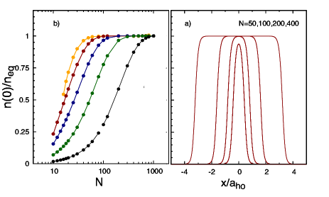
Figure 1: In panel $a)$ we show the evolution of the density profile as the number of the particles in the cloud is increased for the case $a_{1D}=-7000a_{0}$, for some selected cases i.e. $N=50,100,200$ and $400$. In panel $b)$ we show, for several scattering lengths $a_{1d}$, the ratio between the density at the center $n(x=0)$ of the cloud and the equilibrium density reached when the density profile becomes flat as a function of the numbers of particle $N$ in the droplet. Data for scattering lengths $a_{1d}/a_{0}=-6500,-7000,-7500,-8000,-8500$ are shown using orange, dark-red, dark-blue, dark-green and black solid dots respectively. All lines are intended to be guide to the eye.

We verify the $N^{-1}$ scaling hydrodynamic prediction for the breathing mode, showing that $\Omega^{2}_{b}N^{2}$ estimated using sum-rule Eq. 2 saturates to a constant value for large number of particles, in the droplet phase (see Fig. 2).

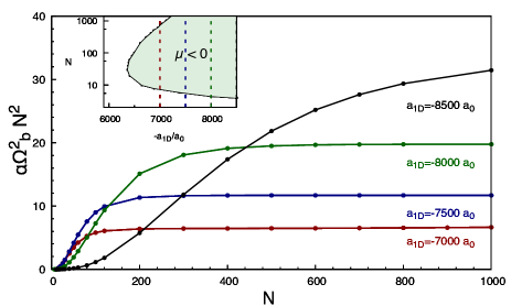
Figure 2: Breathing mode square of the droplet in the absence of trapping potential multiplied by $N^{2}$ for several value of $a_{1D}$. Dark-red, blue, dark-green and black solid dots are estimates of $\Omega_{b}^{2}$ using sum-rule approach from Eq. (2) for $-a_{1D}/a_{0}=7000,7500,8000,8500$ respectively. For each scattering length the values of $\Omega_{b}^{2}$ have been multiplied by a common constant factor $\alpha$ to show easily the constant behaviour in the same figure. In the inset we show the phase diagram for the dipolar system from Ref. Palo et al., 2022, where the self-bound droplet occurs when the chemical potential $\mu<0$. The dashed lines corresponds to the values shown in the main figure with the same color code. All lines are intended to be guide to the eye.

We see in more detail the behaviour of the breathing mode comparing its estimates obtained using the different approximations for a selected scattering length, namely $a_{1D}=-7000a_{0}$, as a function of the number of particles. For $N\gtrsim 100$ we can identify a region, consistent with a flat-top density profile region (see panel $a)$ of Fig.1) where all the three estimates used collapse. The fact that all the approaches quantitatively agrees with each other implies that the response function $\mathrm{Im}\chi(\omega)\sim Z\delta(\omega-\Omega_{b})$, see App. B, and i.e. in this region the breathing mode is sharply defined.

When the number of particles in the cloud is smaller, yet larger than a critical value beyond which the system is not self-bound (in this case roughly $N\simeq 10$ see inset of Fig. 2), the profile density looses the flat-top droplet shape. The phenomenological hydrodynamic approach strongly relies on the assumption that the droplet oscillates while keeping its density uniform (i.e. the droplet shape is a simple rectangle). In the small $N$ region, where the cloud has not achieved a flat-top density profile, the breathing mode grows as $N^{\beta}$ with $\beta>2/3$ where $\beta=2/3$ is the behavior predicted for a solitonic shape density profileAstrakharchik and Malomed (2018). For large number of particles where the droplet shows a flat top, the $N^{-1}$ decay of the breathing mode predicted in Eq. (12) works well but becomes obviously inaccurate when we depart from the simple rectangular shape and it is necessary to retain the whole profile density as in the generalized Gross -Pitaevkii equations (Eq. 27). The two different behaviours of the breathing mode as a function of $N$ produce a maximum that can be interpreted, together with the $N^{-1}$ scaling, as the signature of the development of a dropletAstrakharchik and Malomed (2018); Tylutki et al. (2020); Du et al. (2023).

In Fig. 3 we see that the estimate of the breathing mode based on Eq. (27) is always above the sum-rule estimate Eq. (2) in the whole $N$ range; we expect this hierarchy since the generalized Gross-Pitaevskii estimate is related to the moment ratio $m_{3}/m_{1}$ while the sum-rule is related to the ratio $m_{1}/m_{-1}$, and $m_{3}/m_{1}\geq m_{1}/m_{-1}$ as discussed in App. B.

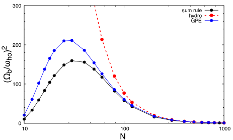
Figure 3: Breathing mode square of the droplet as a function of number of particles $N$ without the trap for $a_{1D}=-7000a_{0}$, divided by the longitudinal frequency consistent with $a_{ho}=24000a_{0}$. Black, blue and red solid dots are estimates for $\Omega_{b}$ using the sum-rule approach Eq.  (2), derivation from Gross-Pitaevskii Eq. (27) and the hydrodynamic approach Eq. (12) respectively. All lines are intended to be guide to the eye.

We conclude this part of the section by commenting on the stability of the cloud and therefore on the possibility of detecting the droplet and this behaviour for an experimental configuration close to the one achieved in Ref. Tang et al., 2018; Kao et al., 2021. We look at the ratio of the breathing-mode frequency to the particle-emission threshold: $-\hbar\Omega_{b}/\mu$ which is shown in Fig. 4 for several scattering lengths as a function of the number of particles in the cloud. When the energies of the collective mode are above the chemical potential, i.e. $-\hbar\Omega_{b}/\mu>1$, exciting the droplet leads to emission of particles. As a consequence the cloud self-evaporates Petrov (2015), a property that might make the system a possible bath for sympathetic cooling for the other system. In a dipolar bosonic gas confined in a cigar-shaped trapBaillie et al. (2017), or in a strictly 1D bosonic mixtureTylutki et al. (2020) the breathing mode was predicted to be always bound.

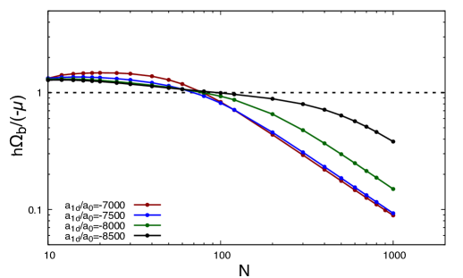
Figure 4: Ratio of breathing mode of the droplet, using the sum-rule approach, and chemical potential as a function of number of particles $N$ without the trap for $-a_{1D}/a_{0}=7000,7500$, $8000$, and $8500$ (Dark-red, blue, dark-green and black solid dots respectively). All lines are intended to be guide to the eye.

By contrast, in the case we are investigating, which is strictly one-dimensional and where besides the dipolar interaction we also have the repulsive contact interaction, we find that for size smaller than $N\simeq 80$ exciting the droplet would imply an evaporation of the cloud itself, that could occur by the fragmentation of the droplet into small pieces. Therefore the increasing scaling of the breathing frequency as a function of $N$, as well as its maximum will not be detectable, while for larger number of particles, yet achieveable, the cloud is stable and this occurs when the flat-top density profile is reached and the $N^{-1}$ behaviour of the breathing mode fullfilled.

III.2 Breathing mode for a trapped system

In this part of the section we analyse how the trapping potential affects the density profile and consequently the breathing mode and if it is possible to detect a scaling law similar to the one obtained for the self-bound droplet. As discussed in the previous section the first effect of the trapping potential is to introduce $\omega_{ho}$ in the breathing potential as the relevant scale as shown in Eq. (16) and Eq. (28).

In Fig. 5 we show a case where there is an appreciable region where the effect of the potential is not so strong and we can appreciate a plateau in the quantity $\Omega_{b}^{2}N^{2}$ that can be related to the region of $N$ for which we observe a flat top behavior in the density profile (see red data in panel $a)$ and $c)$). When $N\gtrsim 1000$ the effect of the trap to the density profile is visible (see panel $d)$), the chemical potential become eventually positive, and we loose the plateau in $\Omega_{b}^{2}N^{2}$.

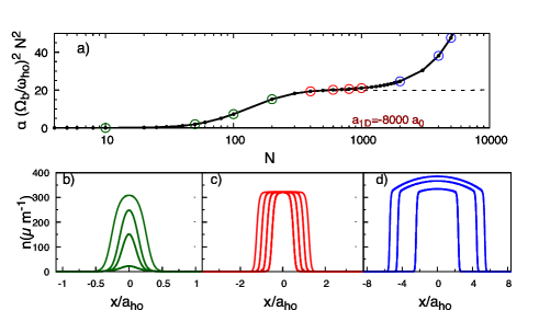
Figure 5: In the upper panel $a)$ we show $\alpha(\Omega_{b}/\omega_{ho})^{2}N^{2}$ for the scattering length $a_{1D}=-8000a_{0}$, where $\alpha$ is a constant multiplicative value. The dashed black curve is the same quantity computed for the system in the absence of trap, it is apparent the constant behavior at large $N$. In the lower panels we show the density profiles of the trapped cloud for different number of particles in different regions. We show profile densities with solid dark-green lines for $N=10,50,100$ and $200$ (panel $b)$, with red solid lines for $N=400,600,800$ and $1000$ (panel $c)$ and with blue solid lines for $N=2000,4000$ and $5000$. Open dots in the upper panel correspond to the results for the density profile shown in the lower panels according to the color code. Lines are intended to be guide to the eye.

The qualitative picture of the breathing mode as a function of the number of particles is similar to the one obtained in the absence of the trapping potential: there is maximum in $\Omega_{b}$ that signals the fact that droplet with a flat-top density profile is developing.

We conclude our analysis by comparing the different approaches for computing the breathing mode for trapped system using, beyond the standard sum-rule approach, Eq. (2), the hydrodynamic expression Eq. (16) and the generalized Gross-Pitaevskii approach Eq. (28). Analogously to the case in the absence of the trap, we observe that breathing-mode estimated by using the sum rule has the lowest value and hierarchy between the estimates of $\Omega_{b}$ is fulfilled as well (App. B).

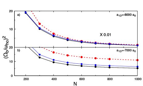
Figure 6: $\Omega^{2}_{b}/\omega^{2}_{ho}$ as a function of number of particles $N$ with the trap for $a_{1D}=-8000a_{0}$ (panel $a)$) and $a_{1D}=-7000a_{0}$ (panel $b)$). Black, blue and red solid dots are estimates for $\Omega_{b}$ using the sum-rule approach Eq. (2), derivation from Gross-Pitaevskii Eq. (28) and the hydrodynamic approach Eq. (12) respectively. All lines are intended to be guide to the eye.

As largely already discussed before, in the absence of trap the breathing mode of the droplets decays as $N^{-1}$ and all the different estimates converge (see fig. 3) once we are in the region where the droplet has a flat-top density profile. We can observe the same kind of collapse only if we are in the flat-top region also with the trapping potential, that means that the effect of the trap is small and therefore Eq. (12) and Eq. (28) are good approximations and the collective mode is well defined. This is clearly shown in Fig. 6, where in panel $a)$ we show $(\Omega_{b}/\omega_{ho})^{2}$ for $a_{1D}/a_{0}=8000$ in a range of $N$ where the flat-top shape of the profile density holds (see Fig. 5) with the appropriate consequences. In this range there in an apparent collapse. However, in the same range of $N$ we can consider a scattering length smaller in absolute value ($a_{1D}/a_{0}=-7000$). In this case the trapping potential affects the profile density shape so we cannot expect the collapse of all derivations (see panel $b)$ of Fig. 6.

IV Conclusions

We have investigated the breathing mode of a quantum droplet in a one-dimensional dipolar Bose gas in a regime close to that experimentally realizedTang et al. (2018); Kao et al. (2021). Our theory relies on a variational calculation of the ground state energy as a function of densityPalo et al. (2020, 2021, 2023). When the dipolar interactions are made attractive, by increasing the scattering length and the number of particles, a soliton-like density profile is obtained with a maximum that scales linearly with the number of particles $N$. Upon further increasing the number of particles, the density acquires a flat-top profile whose maximum does not vary with $N$, indicating the formation of the droplet. Starting with a phenomenological approach, that relies on an idealized rectangular density profile of the droplet, and simple hydrodynamics, we have found that the breathing mode frequency scales as $N^{-1}$. We have then turned to a generalized Gross-Pitaevskii (GGPE) approachKolomeisky et al. (2000); Oldziejewski et al. (2020) that takes into account explicitly density gradients. Finally we have benchmarked the results with the sum-rule approach, in the limit of zero trapping confinement. Of these three methods, the sum rule always gives the lowest estimate, as it links the breathing mode to the lowest moments of the dynamic structure factor. Both the sum-rule and the GGPE give a vanishing breathing frequency at low particle number $N$ and show a maximum of the breathing frequency at intermediate values of $N$. At large value of $N$, they become asymptotic to the hydrodynamic approximation. We have considered the stability of the cloud against particle emission, and we have found that the cloud is stable at $N$ sufficiently large. We have also analyzed the breathing mode of the droplet in the presence of longitudinal trapping. In the presence of the trap the frequency of the breathing mode does not return to zero when increasing the number of particles, saturating to a value that depends on the scattering length. One remark is in order here: While the momentum distribution is the natural observable to investigate the formation of droplets in two or three dimensions where the breaking of the translational symmetry is well established, the quasi-one dimensional case is more delicate because the droplet corresponds to a flat top density and the measure of the breathing mode we propose is more reliable. We believe that our theoretical predictions for quasi-one-dimensional quantum droplets are testable with the available experimental setups of strongly confined gases of dipolar atoms in quasi-one dimensional geometry. In particular, the behavior of the measured breathing mode of the droplet will highlight the reliability and accuracy of the three theoretical methods we have proposed. Finally, we stress that the generalized Gross-Pitaevskii approach developed here could be applied also to droplets forming in other quasi-one-dimensional superfluid systems.

Appendix A Dirac-Frenkel variational method and sum rules

In a second quantized treatment, we can introduce the dilatation operator

$$D=\frac{\hbar}{2i}\int dxx\left(\psi^{\dagger}\frac{\partial\psi}{\partial x}-\frac{\partial\psi^{\dagger}}{\partial x}\psi\right),$$ (29)

and the quadrupole operator

$$Q=\frac{1}{2}\int dxx^{2}\psi^{\dagger}(x)\psi(x),$$ (30)

satisfying the commutation relations

$$[Q,H] = \frac{i\hbar}{m}D,$$ (31)

$$[D,Q] = -2i\hbar Q.$$ (32)

If we consider the annihilation operator $\psi(x)$, the particle density $n(x)$ and the particle current $j(x)$, they transform under a time-dependent dilatation as

$$e^{i\frac{\lambda D}{\hbar}}\psi(x)e^{i\frac{mQ}{\hbar}\frac{d\lambda}{dt}}e^{-i\frac{mQ}{\hbar}\frac{d\lambda}{dt}}e^{-i\frac{\lambda D}{\hbar}} = e^{-i\frac{mx^{2}}{2\hbar}\frac{d\lambda}{dt}}e^{-\lambda/2}\psi(xe^{-\lambda}),$$ (33)

$$e^{i\frac{\lambda D}{\hbar}}e^{-i\frac{mQ}{\hbar}\frac{d\lambda}{dt}}n(x)e^{i\frac{mQ}{\hbar}\frac{d\lambda}{dt}}e^{-i\frac{\lambda D}{\hbar}} = e^{-\lambda}n(xe^{-\lambda}),$$ (34)

$$e^{i\frac{\lambda D}{\hbar}}e^{-i\frac{mQ}{\hbar}\frac{d\lambda}{dt}}j(x)e^{i\frac{mQ}{\hbar}\frac{d\lambda}{dt}}e^{-i\frac{\lambda D}{\hbar}} = e^{-2\lambda}j(xe^{-\lambda})$$

$$+\frac{d}{dt}(e^{-\lambda})xn(xe^{-\lambda}).$$

Choosing as normalized trial wavefunction

$$|\Psi\rangle(t)=e^{\frac{imQ}{\hbar}\frac{d\lambda}{dt}}e^{-i\lambda(t)D/\hbar}e^{-iE_{0}t/\hbar}|0\rangle,$$ (36)

the expectation values of the particle density and current behave as

$$\langle\Psi|\rho(x)|\Psi\rangle = e^{-\lambda}\langle 0|\rho(xe^{-\lambda})|0\rangle=\frac{1}{R}n_{0}\left(\frac{x}{R}\right),$$

$$\langle\Psi|j(x)|\Psi\rangle = e^{-2\lambda}\langle 0|j(xe^{-\lambda})|0\rangle+\frac{d}{dt}(e^{-\lambda})x\langle 0|\rho(xe^{-\lambda})|0\rangle$$ (37)

$$= 0+\frac{mx\dot{R}}{\hbar R^{2}}n_{0}\left(\frac{x}{R}\right),$$

so we recover the ansatz we used for the density in the GGPE with $R(t)=e^{\lambda(t)}$. Moreover, using the representation

$$\psi(x)=e^{i\theta(x)}\sqrt{n(x)}$$ (38)

with $[\theta(x),\rho(x^{\prime})]=i\delta(x-x^{\prime})$ the time dependent rescaling shifts the phase $\theta$ by $mx^{2}\dot{\lambda}(t)/(2\hbar)$ as in the GGPE. Inserting the trial wavefunction (36) in the Dirac-FrenkelDirac (1930); Frenkel (1950) action

$$S=\int dt\left[i\hbar\langle\Psi|\partial_{t}|\Psi\rangle-\langle\Psi|H|\Psi\rangle\right],$$ (39)

we get

$$S=m\langle 0|Q|0\rangle\int dt\left[\frac{d}{dt}(e^{\lambda})\right]^{2}$$

$$-\int dt\langle 0|e^{\frac{i}{\hbar}\lambda D}(H-E_{0})e^{-\frac{i}{\hbar}\lambda D}|0\rangle,$$

and for small oscillations,

$$S=m\langle 0|Q|0\rangle\int dt\left(\frac{d\lambda}{dt}\right)^{2}-\frac{\lambda^{2}}{\hbar^{2}}\int dt\langle 0|D(H-E_{0})D|0\rangle,$$

yielding

$$\Omega_{b}^{2} = \frac{\langle 0|D(H-E_{0})D|0\rangle}{\hbar^{2}\langle 0|Q|0\rangle},$$ (40)

$$= \frac{\langle 0|Q(H-E_{0})^{3}Q|0\rangle}{\langle 0|Q(H-E_{0})Q\rangle},$$

where in the second line, we have used the commutation relations (31)–(32). That last expression can be rewritten as a sum-ruleStringari (1994). Using the imaginary part of the quadrupole-quadrupole response function,

$$\mathrm{Im}\chi_{QQ}(\omega)=\pi\sum_{n}|\langle 0|Q|n\rangle|^{2}\delta(E_{n}-\hbar\omega-E_{0}),$$ (41)

we rewrite our expression

$$\Omega_{b}^{2}=\frac{\int_{0}^{+\infty}d\omega\omega^{3}\mathrm{Im}\chi_{QQ}(\omega)}{\int_{0}^{+\infty}d\omega\omega\mathrm{Im}\chi_{QQ}(\omega)}.$$ (42)

Appendix B Sum rules and Hölder inequality

Sum rules such as (42) or the expressions derived in Ref.Stringari (1994) yield upper bounds for the gap between the ground state and the first excited state having a nonzero matrix element of $Q$ with the ground state

$$E_{1}-E_{0}\leq\Delta(\alpha,\beta)=\left[\frac{\int_{0}^{+\infty}d\omega(\hbar\omega)^{\alpha}\mathrm{Im}\chi_{QQ}(\omega)}{\int_{0}^{+\infty}d\omega(\hbar\omega)^{\beta}\mathrm{Im}\chi_{QQ}(\omega)}\right]^{\frac{1}{\alpha-\beta}}.$$ (43)

These bounds are related to each other by

$$\Delta(\alpha,\beta)^{\alpha-\beta}\Delta(\beta,\gamma)^{\beta-\gamma}=\Delta(\alpha,\gamma)^{\alpha-\gamma},$$ (44)

and in the case of a single mode $\Im\chi(\omega)=A\delta(\omega-\Omega)$, they all lead to $E_{1}-E_{0}\leq\Omega$. With a richer spectrum, the sum rules result in different estimates for the energy of the first excited state. The bounds Eq. (44) depend of the generalized moments

$$m_{\alpha}=\int_{0}^{+\infty}d\omega(\hbar\omega)^{\alpha}\mathrm{Im}\chi_{QQ}(\omega)$$ (45)

of the response function. For $\alpha$ a positive integer, the moment $m_{\alpha}$ can be expressed using only multiple commutators of $Q$ with the Hamiltonian, while for $\alpha=-1$ it can be expressed in terms of the real part of the response function $\chi_{QQ}(\omega=0)$. This makes such bounds convenient since they only depend on quantities computed in the ground state. However, one would like to determine which bounds yield the most accurate estimates for the energy of the excited state. It turns out that using Hölder inequalitiesAbramowitz and Stegun (1972), such hierarchy can be established. If we start from the integral

$$\int_{0}^{+\infty}\frac{d\omega}{\pi}(\hbar\omega)^{x\alpha+(1-x)\gamma}\mathrm{Im}\chi(\omega),$$ (46)

with $0<x<1$ by choosing $p=1/x$ and $q=1/(1-x)$, and applying the Hölder inequalities (3.2.8) or (3.2.10) of Ref.Abramowitz and Stegun (1972) to the functions

$$(\hbar\omega)^{\alpha/p}\left(\mathrm{Im}\chi(\omega)/\pi\right)^{1/p},$$ (47)

and

$$(\hbar\omega)^{\gamma/q}\left(\mathrm{Im}\chi(\omega)/\pi\right)^{1/q},$$ (48)

we find

$$\int_{0}^{+\infty}\frac{d\omega}{\pi}(\hbar\omega)^{x\alpha+(1-x)\gamma}\mathrm{Im}\chi(\omega)\leq\left[\int_{0}^{+\infty}\frac{d\omega}{\pi}(\hbar\omega)^{\alpha}\mathrm{Im}\chi(\omega)\right]^{x}$$

$$\times\left[\int_{0}^{+\infty}\frac{d\omega}{\pi}(\hbar\omega)^{\gamma}\mathrm{Im}\chi(\omega)\right]^{(1-x)}.$$ (49)

Such inequality, inserted in Eq. (43), results in

$$\Delta(\alpha,\alpha x+\gamma(1-x))\geq\Delta(\alpha x+\gamma(1-x),\gamma).$$ (50)

In particular, with $\alpha>\beta>\gamma$, setting $x=(\beta-\gamma)/(\alpha-\gamma)$, we get $\Delta(\alpha,\beta)\geq\Delta(\beta,\gamma)$. Then, by inserting this inequality in Eq. (44), we obtain $\Delta(\alpha,\beta)\geq\Delta(\alpha,\gamma)\geq\Delta(\beta,\gamma)$, so more accurate estimates are obtained with lower values of the exponents in Eq. (43). In particular, the estimate given by Eq. (42), that is $\alpha=3,\beta=1$ in Eq. (43), is always above the one with $\alpha=1,\beta=-1$ from Ref. Chiofalo et al. (1996); Menotti and Stringari (2002). Obviously, when the difference between the two approximations becomes large, it is an indication that the breathing mode is not sharply defined. So, by comparing the results of the two approximations, we can identify the regions of the phase diagram where a well defined breathing mode can be observed.

Appendix C Deformation of the droplet

When the condition $\omega_{0}\ll\Omega_{b}$ is not fulfilled, we must take into account the deformation of the droplet by the harmonic trapping. This can be done using a local density approximationDe Palo et al. (2008). The density in the system at rest is given by

$$e^{\prime}(\rho_{\mathrm{eq}}(x))=\mu-V(x),$$ (51)

but we have alsoPalo et al. (2022) $e(\rho)\geq e^{\prime}(\rho_{1})\rho$, and $E-\mu N\geq\int[e^{\prime}(\rho_{1})+V(x)-\mu]\rho(x)dx$. So when $V(x)>\mu-e^{\prime}(\rho_{1})$, we can minimize energy by setting $\rho_{\mathrm{eq}}(x)=0$. We have therefore a discontinuous drop of the density from $\rho_{1}$ to zero at $x=\pm L/2$, and $V(L/2)=\mu-e^{\prime}(\rho_{1})$. At the center of the trap, the density is given by $e^{\prime}(\rho_{\mathrm{eq}}(0))=\mu$ and the number of particles is

$$N = \sqrt{\frac{2}{m\omega_{0}^{2}}}\left[\rho_{1}\sqrt{e^{\prime}(\rho_{\mathrm{eq}}(0)-e^{\prime}(\rho_{1})}\right.$$ (52)

$$\left.+\int_{\rho_{1}}^{\rho_{\mathrm{eq}}(0)}\sqrt{e^{\prime}(\rho_{\mathrm{eq}}(0))-e^{\prime}(\rho)}d\rho\right]$$

Hydrodynamic equationsMenotti and Stringari (2002); De Palo et al. (2008) can be derived from the Hamiltonian

$$H=\int_{-L/2}^{L/2}\left[\frac{\rho_{\mathrm{eq}}(x)}{2m}(\partial_{x}\theta)^{2}+e^{\prime\prime}(\rho_{\mathrm{eq}}(x))\frac{(\delta\rho)^{2}}{2}\right],$$ (53)

with commutation relations $[\theta(x),\delta\rho(y)]=-i\delta(x-y)$. The field $\theta(x,t)$ is a velocity potential, while $\delta\rho(x,t)$ is the deviation of the local density from its equilibrium value. In general, an ansatz of the form Eq. (6 corresponds to $\theta(x,t)=\epsilon(t)x^{2}/2$. The continuity equation still leads to an ansatz compatible with Eq. (4) for $\delta\rho(x,t)$, but in general, the Euler equation cannot be satisfied. Nevertheless, we can introduce the Lagrangian

$$\mathcal{L}_{\mathrm{hydro}}=\int dx\left[\frac{(\partial_{t}\theta)^{2}}{2e"(\rho_{\mathrm{eq}}(x))}-\frac{\rho_{\mathrm{eq}}(x)(\partial_{x}\theta)^{2}}{2m}\right],$$ (54)

and use the form $\theta(x,t)=\epsilon(t)x^{2}/2$ as a variational ansatz in the action.

Appendix D Properties of the ground state wavefunction of the Generalized GPE

The ground state wavefunction of the generalized GPE satisfies

$$-\frac{\hbar^{2}}{2m}\frac{d^{2}\psi_{0}}{dx^{2}}+[e^{\prime}(\psi_{0}^{2})+V(x)-\mu]\psi_{0}=0.$$ (55)

Multiplying Eq.(55) by $\psi_{0}$, we find

$$-\frac{\hbar^{2}}{2m}\frac{d}{dx}\left(\psi_{0}\frac{d\psi_{0}}{dx}\right)+\frac{\hbar^{2}}{2m}\left(\frac{d\psi_{0}}{dx}\right)^{2}+[e^{\prime}(\psi_{0}^{2})+V(x)-\mu]\psi_{0}^{2}=0,$$ (56)

while multiplying Eq.(55) by $d\psi_{0}/dx$ and integrating, yields

$$e(\psi_{0})^{2}+[V(x)-\mu]\psi_{0}^{2}-\frac{\hbar^{2}}{2m}\left(\frac{d\psi_{0}}{dx}\right)^{2}=\int_{-\infty}^{x}m\omega_{0}^{2}y\psi_{0}(y)^{2}dy.$$ (57)

Using Eq. (56), we can eliminate $(V(x)-\mu)\psi_{0}^{2}$ in Eq. (56). By integrating the resulting equation from $-\infty$ to $+\infty$, we obtain

$$\int_{-\infty}^{+\infty}dx\left[\frac{\hbar^{2}}{m}\left(\frac{d\psi_{0}}{dx}\right)^{2}+e^{\prime}(\psi_{0}^{2})\psi_{0}^{2}-e(\psi_{0}^{2})\right]$$

$$+\int_{-\infty}^{+\infty}dxm\omega_{0}^{2}\int_{-\infty}^{x}dyy\psi_{0}(y)^{2}=0.$$ (58)

Using an integration by parts in the second line, we finally obtain

$$\int dx\left[\frac{\hbar^{2}}{m}\left(\frac{d\psi_{0}}{dx}\right)^{2}+e^{\prime}(\psi_{0}^{2})\psi_{0}^{2}-e(\psi_{0}^{2})-m\omega_{0}^{2}x^{2}\psi_{0}(x)^{2}\right]=0.$$ (59)

After substituting $\psi_{0}(x)=\sqrt{n_{0}(x)}$, we see that the condition above reduces to Eq.(II.2) with $R(t)=1,\forall t$.

References

- Lauriane Chomaz et al. (2023) F. F. Lauriane Chomaz, Igor Ferrier-Barbut, B. L. L. Bruno Laburthe-Tolra, and T. Pfau, Rep. Prog. Phys. 86, 026401 (2023).
- Schmitt et al. (2016) M. Schmitt, M. Wenzel, F. Böttcher, I. Ferrier-Barbut, and T. Pfau, Nature 539, 259 (2016).
- Kadau et al. (2016) H. Kadau, M. Schmitt, M. Wenzel, C. Wink, T. Maier, I. Ferrier-Barbut, and T. Pfau, Nature 530, 194 (2016).
- Chomaz et al. (2016) L. Chomaz, S. Baier, D. Petter, M. J. Mark, F. Wächtler, L. Santos, and F. Ferlaino, Phys. Rev. X 6, 041039 (2016).
- Böttcher et al. (2019) F. Böttcher, M. Wenzel, J.-N. Schmidt, M. Guo, T. Langen, I. Ferrier-Barbut, T. Pfau, R. Bombín, J. Sánchez-Baena, J. Boronat, et al., Phys. Rev. Res. 1, 033088 (2019).
- Oldziejewski et al. (2020) R. Oldziejewski, W. Górecki, K. Pawlowski, and K. Rzazewski, Phys. Rev. Lett. 124, 090401 (2020).
- Palo et al. (2021) S. D. Palo, E. Orignac, M. Chiofalo, and R. Citro, Phys. Rev. B 103, 115109 (2021).
- Palo et al. (2022) S. D. Palo, E. Orignac, and R. Citro, Phys. Rev. B 106, 014503 (2022).
- Cabrera et al. (2018) C. Cabrera, L. Tanzi, J. Sanz, B. Naylor, P. Thomas, P. Cheiney, and L. Tarruell, Phys. Rev. Lett. 93, 050401 (2018).
- Semeghini et al. (2018) G. Semeghini, G. Ferioli, L. Masi, C. Mazzinghi, L. Wolswijk, F. Minardi, M. Modugno, G. Modugno, M. Inguscio, and M. Fattori, Phys. Rev. Lett. 120, 235301 (2018).
- D’Errico et al. (2019) C. D’Errico, A. Burchianti, M. Prevedelli, L. Salasnich, F. Ancilotto, M. Modugno, F. Minardi, and C. Fort, Phys. Rev. Res. 1, 033155 (2019).
- Haller et al. (2009) E. Haller, M. Gustavsson, M. Mark, J. G. Danzl, R. Hart, H. C. Naegerl, and G. Pupillo, Science 325, 1224 (2009).
- Wächtler and Santos (2016) F. Wächtler and L. Santos, Phys. Rev. A 94, 043618 (2016), eprint 1605.08676.
- Baillie et al. (2017) D. Baillie, R. M. Wilson, and P. B. Blakie, Phys. Rev. Lett. 119, 255302 (2017).
- Pal et al. (2022) S. Pal, D. Baillie, and P. B. Blakie, Phys. Rev. A 105, 023308 (2022).
- Tang et al. (2018) Y. Tang, W. Kao, K.-Y. Li, S. Seo, K. Mallayya, M. Rigol, S. Gopalakrishnan, and B. L. Lev, Phys. Rev. X 8, 021030 (2018).
- Kao et al. (2021) W. Kao, K.-Y. Li, K.-Y. Lin, S. Gopalakrishnan, and B. L. Lev, Science 371, 296 (2021).
- Palo et al. (2020) S. D. Palo, R. Citro, and E. Orignac, Phys. Rev. B 101, 045102 (2020).
- Palo et al. (2023) S. D. Palo, E. Orignac, R. Citro, and L. Salasnich, Condens. Matter 8, 26 (2023).
- Menotti and Stringari (2002) C. Menotti and S. Stringari, Phys. Rev. A 66, 043610 (2002).
- Hu et al. (2014) H. Hu, G. Xianlong, and X.-J. Liu, Physical Review A 90, 013622 (2014).
- Choi et al. (2015) S. Choi, V. Dunjko, Z. D. Zhang, and M. Olshanii, Phys. Rev. Lett. 115, 115302 (2015).
- Chen et al. (2015) X.-L. Chen, Y. Li, and H. Hu, Physical Review A 91, 063631 (2015).
- Gudyma et al. (2015) A. I. Gudyma, G. E. Astrakharchik, and M. B. Zvonarev, Phys. Rev. A 92, 021601 (2015).
- (25) By solving the time-dependent generalized Gross-Pitaevskii equation, we have verified that, after initially exciting the mode by external radial compression of the trap, in the limit .
- Girardeau (1960) M. Girardeau, J. Math. Phys. 1, 516 (1960).
- Kolomeisky et al. (2000) E. B. Kolomeisky, T. J. Newman, J. P. Straley, and X. Qi, Phys. Rev. Lett. 85, 1146 (2000).
- Dunjko et al. (2001) V. Dunjko, V. Lorent, and M. Olshanii, Phys. Rev. Lett. 86, 5413 (2001).
- Öhberg and Santos (2002) P. Öhberg and L. Santos, Phys. Rev. Lett. 89, 240402 (2002).
- Dirac (1930) P. A. M. Dirac, Mathematical Proceedings of the Cambridge Philosophical Society 26, 376 (1930).
- Frenkel (1950) Y. Frenkel, Wave mechanics: advanced general theory (Dover Publications, New York, 1950).
- Astrakharchik and Malomed (2018) G. E. Astrakharchik and B. A. Malomed, Phys. Rev. A 98, 013631 (2018).
- Tylutki et al. (2020) M. Tylutki, G. E. Astrakharchik, B. A. Malomed, and D. S. Petrov, Phys. Rev. A 101, 051601 (2020).
- Du et al. (2023) X. Du, Y. Fei, X.-L. Chen, and Y. Zhang, Phys. Rev. A 108, 033312 (2023).
- Petrov (2015) D. Petrov, Phys. Rev. Lett. 115, 155302 (2015).
- Stringari (1994) S. Stringari, Phys. Rev. B 49, 6710 (1994).
- Abramowitz and Stegun (1972) M. Abramowitz and I. Stegun, eds., Handbook of mathematical functions (Dover, New York, 1972).
- Chiofalo et al. (1996) M. L. Chiofalo, S. Conti, and M. P. Tosi, J. Phys.: Condens. Matter 8, L1921 (1996).
- De Palo et al. (2008) S. De Palo, E. Orignac, R. Citro, and M. L. Chiofalo, Phys. Rev. B 77, 212101 (2008).