Radius selection using kernel density estimation for the computation of nonlinear measures

Abstract

When nonlinear measures are estimated from sampled temporal signals with finite-length, a radius parameter must be carefully selected to avoid a poor estimation. These measures are generally derived from the correlation integral which quantifies the probability of finding neighbors, i.e. pair of points spaced by less than the radius parameter. While each nonlinear measure comes with several specific empirical rules to select a radius value, we provide a systematic selection method. We show that the optimal radius for nonlinear measures can be approximated by the optimal bandwidth of a Kernel Density Estimator (KDE) related to the correlation sum. The KDE framework provides non-parametric tools to approximate a density function from finite samples (e.g. histograms) and optimal methods to select a smoothing parameter, the bandwidth (e.g. bin width in histograms). We use results from KDE to derive a closed-form expression for the optimal radius. The latter is used to compute the correlation dimension and to construct recurrence plots yielding an estimate of Kolmogorov-Sinai entropy. We assess our method through numerical experiments on signals generated by nonlinear systems and experimental electroencephalographic time series.

Keywords Nonlinear measures; correlation sum; correlation dimension; Kolmogorov-Sinai entropy; kernel density estimation; recurrence plots.

1 Introduction

Nonlinearity and chaos govern a wide variety of systems. They are found in neurons firing patterns (Faure and Korn, 2001) and related electrophysiological signals (Freeman, 2003), and in unpredictable changes of Earth climate (Ghil et al., 2008), to cite few examples. Nonlinear measures of such systems are made more accurate thanks to an increasing interest in numerical tools suitable for nonlinear phenomena. Indeed, data generated by such systems are more suitable to nonlinear time series analysis, which provide complementary information to traditional linear methods such as power spectrum analysis (Yang et al., 2018).

Our work focuses on estimating various metrics, measures (in the sense of quantitative indices), and invariants that rely on the computation of a correlation sum. The correlation sum is the estimator of the correlation integral, which is the mean probability that two points of the phase space trajectory of a dynamical system are neighbors (Ott, 2002), i.e. the mean probability that their distance is less than a parameter called radius, threshold or tolerance depending on the application domain. The correlation sum captures important aspects of the nonlinear dynamics. Therefore, it is a fundamental quantity in various nonlinear measures: correlation dimension (Grassberger and Procaccia, 1983a), Kolmogorov-Sinai entropy (Grassberger and Procaccia, 1983b; Eckmann and Ruelle, 1985; Faure and Korn, 1998), its approximate versions ApEn (Pincus, 1991) and SampEn (Richman and Moorman, 2000), Rényi’s entropies (Principe, 2010; Singh and Príncipe, 2011), recurrence plots (Eckmann et al., 1987), (Marwan et al., 2007) and related metrics of recurrence quantification analysis (Grendár et al., 2013), etc.

In different nonlinear measures, the radius appears either as a variable or as a parameter. For instance, the correlation dimension is computed by estimating a scaling factor on a logarithmic plot of the correlation sum versus the radius. In contrast, a recurrence plot displays neighboring points on a black and white image and requires to fix the radius parameter beforehand. In both cases, the radius is selected as small as possible. As a correlation sum computed from a finite-length time series will likely tend to 0 together with the radius parameter, the challenge is to identify a radius range corresponding to a statistically useful distribution of neighbors. Eckmann and Ruelle (Eckmann and Ruelle, 1985) (Section V.A.1.a.) refer to it as a “meaningful range” for the radius parameter. In our approach, we first derive an expression of the optimal radius. Then, we introduce a range to select a radius parameter or to study the properties of a function of the radius.

Several empirical rules exist to select a value or a range of values for the radius; however, they generally focused on a particular nonlinear measure (Webber and Marwan, 2015; Zbilut and Webber Jr, 1992; Pincus, 1991). Here, we introduce a method which can be applied to any nonlinear measure derived from the correlation sum. Observing that log-correlation sums are particularly used in nonlinear indices and that relative error arises from logarithmic error terms, we focus on minimizing a relative error between the correlation sum and the correlation integral. We show that minimizing the relative error term is equivalent to minimizing a well-known error used in the framework of Kernel Density Estimation (KDE), widely studied in statistics (Silverman, 1986) and in signal processing (Gunduz and Principe, 2009; Singh and Príncipe, 2011).

KDE denotes a family of non-parametric density estimation methods which generalize the well-known histogram methods (Silverman, 1986). Simple probability functions called kernels are placed at sample data points to approximate the underlying density function. In the KDE framework, the choice of the kernel width influences the degree of smoothing of the estimated density function. Selecting the kernel width is known as the bandwidth selection problem. The latter can be formulated simply as a bias-variance trade-off. Bandwidth selection is an extensively studied problem (see (Jones et al., 1996) for a brief review) with notable usages in signal processing, e.g. mutual information estimation (Moon et al., 1995). The convergence of kernel density estimators for mixing dynamical systems was recently shown in (Hang et al., 2018).

The relation between kernel density estimation and the correlation sum is noted in (Yu et al., 2000) to estimate dynamical invariants in noisy situations. More recently, Gaussian kernels estimators of the correlation integral are applied to estimate Rényi’s entropies (Principe, 2010; Singh and Príncipe, 2011; Erdogmus and Principe, 2006). Here, KDE is used not to derive new estimators of nonlinear measures but rather as a framework providing a systematic rule to select the radius in computing nonlinear measures. We show that the radius minimizing the relative error of the correlation sum estimator is equivalent to the bandwidth minimizing the Mean Integrated Squared Error (MISE) of a density estimator (Section 3.1). Therefore, we use a bandwidth selection method from KDE to derive a closed-form expression for the optimal radius (Section 3.2) and define a “meaningful range” for the radius variable relatively to our optimum (Section 3.3). We conduct numerical experiments on well-known dynamical systems. First, we study the behavior of the correlation sum estimator in the “meaningful range” for signals of different lengths and noise levels (Section 4). Then, we estimate the Kolmogorov-Sinai entropy of both simulated and real signals, using recurrence plots computed with an optimal radius (Section 5).

2 Correlation sum and correlation dimension

Let $(\mathcal{X},\mathcal{A},\mu,T)$ be a measure-preserving dynamical system with $\mathcal{X}\subset\mathbb{R}^{d}$ and $\mu$ the invariant measure (probability distribution in the phase space invariant upon the dynamics). The correlation integral $c(r)$ is the mean probability to find a pair of points at two different time $x,y\in\mathcal{X}$ arbitrarily close, such that the distance between $x$ and $y$ is less than a small radius parameter $r$ (Ott, 2002; Singh and Príncipe, 2011):

$$c(r)={\mathbb{P}}\left((x,y):\|x-y\|_{p}<r\right)=\int\limits_{x\in\mathcal{X}}\mu(B_{r}(x))d\mu(x)$$ (1)

where $B_{r}(x)=\{y\in\mathcal{X}:\|x-y\|_{p}<r\}$ is the generalized $d$-dimensional ball in $L_{p}$ space, with radius $r$ and center $x$. In practice, an estimator of the correlation integral can be computed from a sample trajectory $x_{i}\in\mathbb{R}^{d},1\leq i\leq n$ (Grassberger and Procaccia, 1983a):

$$C(r,n)=\frac{1}{n^{2}}\sum\limits_{i,j=1}^{n}\Theta(r-\|x_{i}-x_{j}\|_{p})\xrightarrow[n\to\infty]{}c(r)$$ (2)

where $\Theta$ is Heaviside step function and $C(r,n)$ is called the correlation sum (Pesin, 2008; Grassberger and Procaccia, 1983a). For small values of $r$, the correlation integral grows as a power law:

$$c(r)\approx\text{const}\times r^{D_{2}}$$ (3)

The quantity $D_{2}$ is called the correlation dimension.

3 Kernel density estimation

A probability density function $f$ may be estimated by placing smoothing kernels at each sample point. A smoothing kernel $K$ is defined as a valid probability density function, which satisfies (Silverman, 1986):

$$\int K(u)du=1 \forall u\in\mathbb{R},K(u)\geq 0$$ (4)

Without loss of generality, we introduce a scaled version of the kernel with a $L_{p}$ norm and a scaling factor $h>0$, $K_{h}(u)=h^{-d}K(u/h)$, which is a valid kernel when $K$ is a valid kernel. A simple kernel is the uniform or boxcar kernel, which remains constant over a domain:

$$K_{h}(u)=\frac{1}{\tau_{p,d}h^{d}}\Theta(h-\|u\|_{p})$$ (5)

where $\Theta$ is Heaviside step function and $\tau_{p,d}$ is the volume of the unit ball defined by the norm $p$ in a $d$-dimensional space (see Appendix A). Given samples $x_{i}\in\mathbb{R}^{d},1\leq i\leq n$, distributed according to a density $f$, a kernel density estimator of $f$ is:

$$\hat{f}_{h}(x)=n^{-1}\sum\limits_{i=1}^{n}K_{h}(x-x_{i})$$ (6)

While kernel density estimators are consistent for i.i.d. samples, independence between consecutive samples cannot generally be assumed for dynamical systems. Hang  et al. (Hang et al., 2018) showed that kernel density estimators are also consistent for dynamical systems with mixing properties and weakly-continuous density function (more specifically $\mathcal{C}$-mixing systems with pointwise $\alpha$-Hölder controllable density, see (Hang et al., 2018) defs. 1 and 2).

The bandwidth parameter $h$ determines the “width” of the kernels and consequently the degree of smoothing of the estimator. A plethora of methods exist to select the bandwidth parameter, see (Jones et al., 1996). Among existing bandwidth selection methods, minimizing the Asymptotic Mean Integrated Squared Error (AMISE), a Taylor expansion of the MISE of the estimator $\mathbb{E}[\int_{\mathbb{R}^{d}}(f(x)-\hat{f}(x))^{2}dx]$, is appealing for practical applications as it allows to derive a closed-form expression of an approximately optimal bandwidth (Silverman, 1986):

$$h_{\text{AMISE}}=\left[\dfrac{W_{1}(K)\times d}{n\times\left[W_{2}(K)\right]^{2}\times W_{1}(\nabla^{2}f)}\right]^{1/(d+4)}$$ (7)

where the functionals $W_{i}$ are defined as $W_{1}(g)=\int_{\mathbb{R}^{d}}g^{2}(x)dx$ and $W_{2}(g)=\int_{\mathbb{R}^{d}}x_{1}^{2}g(x)dx$, where $x_{1}$ is a scalar component of $x$. Reference rules (Silverman, 1986; Scott, 1979) can be easily obtained by replacing the unknown quantity $W_{1}(\nabla^{2}f)$ with the quantity computed using a reference distribution, generally a Gaussian distribution.

4 A reference rule for the optimal radius

To derive the expression of an optimal radius, we proceed as follows. First, we show that the radius minimizing the relative error of the correlation sum estimator is equivalent to the bandwidth minimizing the MISE of a particular density estimator. Second, we derive the closed-form expression of the radius minimizing the AMISE of the estimator. Finally, we identify a meaningful range to select a variable radius.

4.1 Criterion to select the radius

The correlation integral, $c(r)=\mathbb{E}_{\mu}\left[\mu(B_{r}(x))\right]$, is generally estimated by the correlation sum, $\hat{C}(r,n)=n^{-1}\sum_{i=1}^{n}\hat{\mu}(B_{r}(x_{i}))$ ((1) and (2)). To obtain a good estimation of the correlation sum, we shall minimize the error between an estimator of the invariant measure of a ball , $\hat{\mu}(B_{r}(x))$, and the true quantity $\mu(B_{r}(x))$. However, minimizing such error is not sufficient to provide a good estimation for small $r$: the scale of the error decreases with $r$ and systematically leads to the trivial solution $r=0$. Indeed, when $r$ decreases, the absolute error decreases while the relative error is multiplied by a factor proportional to $1/r$ ((3)) and consequently blows up. Therefore, we want to find the radius minimizing a relative error criterion on $\hat{\mu}(B_{r}(x))$. Let $\lambda$ be the Lebesgue measure, such that $\lambda(B_{r})$ is the volume of a ball with radius $r$. We use the fact that $\mu(B_{r}(\cdot))$ is proportional to $r$ (see (Eckmann and Ruelle, 1985), Section V.A.) and consequently that $\mu(B_{r}(\cdot))\propto\lambda(B_{r})$ to simplify the expression of the relative error and express the following local relative error:

$$L(r,x)=\mathbb{E}\left[\left(\frac{\mu(B_{r}(x))-\hat{\mu}(B_{r}(x))}{\lambda(B_{r})}\right)^{2}\right]$$ (8)

where the expectation is taken over samples used to construct the estimator. Given a fixed $r$, $\mu(B_{r}(\cdot))$ is a bounded function on $\mathcal{X}$. We denote $\rho$ the normalized density of $\mu(B_{r}(\cdot))$, such that

$$\rho(x)=\frac{\mu\left(B_{r}(x)\right)}{\int_{\mathcal{X}}\mu(B_{r}(x))dx}=\frac{\mu\left(B_{r}(x)\right)}{\lambda(B_{r})}$$ (9)

and, similarly, $\hat{\rho}_{r}(x)=\hat{\mu}(B_{r}(x))/\lambda(B_{r})$ the estimator of the normalized density $\rho$. After replacing in (8), we obtain:

$$L(r,x)=\mathbb{E}\left[\left(\rho(x)-\hat{\rho}_{r}(x)\right)^{2}\right]$$ (10)

Then, integrating (10) over possible values of $x$ gives a global criterion to select the optimal radius $r_{\text{opt}}$:

$$r_{\text{opt}} =\operatorname*{arg\,min}_{r}\mathcal{L}(r)$$ (11)

where

$$\mathcal{L}(r) =\int_{\mathcal{X}}\mathbb{E}\left[\left(\rho(x)-\hat{\rho}_{r}(x)\right)^{2}\right]dx$$ (12)

With simple manipulations, we see that (12) is indeed the MISE between the estimator of the normalized density $\hat{\rho}_{r}$ and the true normalized density $\rho$ (Silverman, 1986). Finally, $\hat{\rho}_{r}$ can be identified by replacing $\hat{\mu}(B_{r}(x))$ with $\hat{\rho}_{r}$ in the expression of the correlation sum estimator ((2)):

$$C(r,n) =\frac{\lambda(B_{r})}{n}\sum_{i=1}^{n}\hat{\rho}_{r}(x_{i})=\frac{1}{n^{2}}\sum_{i,j=1}^{n}\Theta(r-\|x_{i}-x_{j}\|)$$

yielding

$$\hat{\rho}_{r}(x) =\frac{1}{n\lambda(B_{r})}\sum_{i=1}^{n}\Theta(r-\|x-x_{i}\|)$$ (13)

As $\lambda(B^{p,d}_{r})=\lambda(B^{p,d}_{1})r^{d}$ (A), we observe that $\hat{\rho}_{r}$ is a kernel density estimator with a uniform kernel and a bandwidth parameter $r$ ((5)). Hence, it follows from (11) that the bandwidth minimizing the MISE of the estimator $\hat{\rho}_{r}$ can provide a good approximation of the optimal radius $r_{\text{opt}}$ minimizing the relative error on the correlation sum estimator. Moreover, the AMISE method ((7)) can be used to approximate $r_{\text{opt}}$ with a simple, closed-form expression that resembles to the empirical rules currently used. In the next section, we use the AMISE minimization method to derive a reference rule for the optimal radius.

4.2 Derivation of a reference rule for the optimal radius

As presented in section 3, a Taylor expansion of the MISE can be used to derive a closed-form expression of the optimal bandwidth for an estimator. A particular interest for this method is motivated by the possibility of deriving a closed-form expression of the optimal bandwidth. We use a reference Gaussian distribution in (7) and derive the expressions for $W_{1}(K)$ and $W_{2}(K)$ for the uniform kernel (see Appendix B). Then, substituting these expressions into (7) gives the main result of the paper: a reference rule radius $r_{\text{opt}}$ defined as

$$r_{\text{opt}} =\alpha_{p,d}\times\hat{s}\times n^{-1/(d+4)}$$ (14)

where $\alpha_{p,d}$, depending on the norm and dimension, rescales $r_{\text{opt}}$; $\hat{s}$ is an estimate of the spread of data; and $n$ is the length of the trajectory in phase space.

Remark 1.

In practice, the phase space is reconstructed using a time delay embedding procedure (according to Takens theorem (Takens, 1981)) ; hence, if $N$ denotes the length of the univariate time series, $d$ the embedding dimension and $\tau$ the delay, the length of the trajectory in reconstructed phase space is $n=N-(d-1)\tau$.

4.2.1 Estimation of the spread $\hat{s}$

A first choice for the spread $\hat{s}$ is the average marginal sample standard deviation, defined by $\hat{\sigma}=\sqrt{d^{-1}\sum_{i}S_{i,i}}$, $S\in\mathbb{R}^{d\times d}$ is the sample covariance matrix. When the $d$-dimensional sample is constructed from an univariate time series using delay embedding, components on the diagonal of the sample covariance matrix are equal: $\hat{\sigma}$ is then the sample standard deviation of the time series. Alternatively, as the interquartile range IQR is a good alternative to standard deviation for non-Gaussian data (see (Silverman, 1986) for discussion), a common choice for $\hat{s}$ is:

$$\hat{s}=\min\left(\hat{\sigma},\dfrac{\mathrm{IQR}}{1.34}\right).$$ (15)

4.2.2 Derivation of the reference factor $\alpha_{p,d}$

The expression for the 1-dimensional reference factor is relatively straightforward: $\alpha_{p,1}=(12\sqrt{\pi})^{1/5}\approx 1.843$. The general closed-form expression for $\alpha_{p,d}$ is more complex (see Appendix B, (35)); however, the expression can be simplified for common norms (Appendix C):

$$\alpha_{1,d} =\left[\left(d+2\right)!\,(d+1)(\sqrt{\pi})^{d}\right]^{1/(d+4)}$$ (16)

$$\alpha_{2,d} =2\times\left[\frac{\Gamma\left(\frac{d}{2}+2\right)}{2}\right]^{1/(d+4)}$$ (17)

$$\alpha_{\infty,d} =\left[\frac{36(\sqrt{\pi})^{d}}{d+2}\right]^{1/(d+4)}$$ (18)

Moreover, $\alpha_{p,d}$ is to be computed only once for common dimensions and norms. Hence, we report in Table 1 some values of $\alpha_{p,d}$ that can be used in (14).

$\alpha_{p,d}$		$p$
		1	2	$\infty$
$d$	1	1.843	1.843	1.843
	2	2.468	2.000	1.745
	3	3.087	2.150	1.694
	4	3.705	2.294	1.666
	5	4.325	2.432	1.649

Table 1: Rounded values of the coefficient $\alpha_{p,d}$ for common norms and dimensions. The values can directly be used in reference rule radius, $r_{\text{opt}}=\alpha_{p,d}\times\min\left(\hat{\sigma},\mathrm{IQR}/1.34\right)\times n^{-1/(d+4)}$.

4.3 Identification of a meaningful range for a variable radius

As discussed above, some nonlinear indices require selecting the range of radius values in which the quantity is estimated. For instance, this applies to nonlinear indices quantifying a scaling exponent of the form $\lim\limits_{r\to 0}\frac{\log\nu(B_{r})}{\log r}$ (with $\nu$ a (with nu a probability distribution in the phase space), as often encountered in the chaotic systems literature (see e.g. (Pesin, 2008; Ott, 2002)). In practice, the limit ${r\to 0}$ is generally intractable, and estimations of $\nu$ for small $r$ are highly variable due to poor statistics (Eckmann and Ruelle, 1985). On the other hand, at a certain point, large $r$ will not capture the desired scaling effect. Hence, there is a range of values which must be selected to support a good estimation of the nonlinear measure. Here, we introduce our arguments to guide the selection of a meaningful range for a variable radius.

The AMISE can be expanded in an integrated squared bias and integrated variance of the density estimator, giving the following expressions of bias and variance as functions of $r$ (Silverman, 1986):

$$\mathrm{bias}(r) \simeq\frac{r^{2}}{2}W_{2}(K)\nabla^{2}\rho(x)$$ (19)

$$\mathrm{var}(r) \simeq\frac{W_{1}(K)}{nr^{d}}\rho(x)$$ (20)

The behavior of the relative error with $r$ can be understood from (19) and (20): the bias is proportional to $r$ whereas the variance is inversely proportional to $r$. As $r_{\text{opt}}$ minimizes the AMISE, the bias contribution increases with $r$ while the variance decreases with $r$. However, the bias term only depends on $r$ whereas the variance term decreases when the number of points increases. This observation –considering that usually the bandwidth minimizing the AMISE is too large, suggests selecting the optimal radius $r_{\text{opt}}$ as the upper bound for the meaningful range. We introduce a range parameter $0<\beta<1$ to select the lower bound as a fraction of $r_{\text{opt}}$, such that the radius values lie within the range:

$$\mathcal{R}=\left[\beta r_{\text{opt}},r_{\text{opt}}\right]$$ (21)

Due to the relations (19) and (20), we argue that the value of $\beta$ shall be decreased when increasing the number of points.

5 Estimation of the correlation dimension

In the following, we investigate the behavior of the Grassberger and Proccacia algorithm for the estimation of the correlation dimension. We compare the spread and bias of estimations in the full range of available scales with estimations in the meaningful range derived in Section 4.3.

5.1 The Grassberger and Proccacia algorithm

The correlation dimension $D_{2}$ can be expressed as:

$$D_{2}=\lim\limits_{r\to 0}\dfrac{\log c(r)}{\log r}=\lim\limits_{r\to 0}\lim\limits_{n\to\infty}\dfrac{\log C(r,n)}{\log r}$$ (22)

The Grassberger and Proccacia algorithm (Grassberger and Procaccia, 1983a) for the empirical estimation of the correlation dimension consists in computing the correlation sum for different values of $r$ and plotting $\log C(r,n)$ versus $\log r$. The slope of the linear region in this logarithmic plot provide the desired estimation of the correlation dimension $D_{2}$ (Ott, 2002). Similarly to the original paper (Grassberger and Procaccia, 1983a), we use linear regression to estimate the slope.

5.2 Procedure for generating reconstructed trajectories

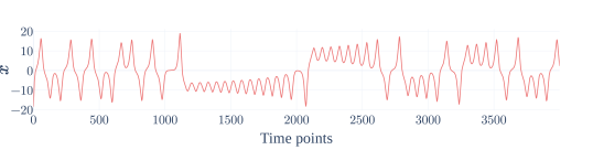
((a))

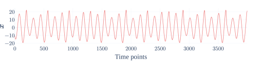
((b))

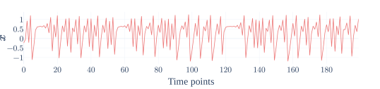
((c))

Figure 1: Sample series for the Lorenz attractor (1(a)), the Rössler attractor (1(b)) and the Hénon map (1(c)). Series from the $x$ coordinates were systematically used to reconstruct the trajectory using Takens delay embedding.

We conducted numerical experiments on the Lorenz system (Lorenz, 1963) ($\sigma=10$, $\beta=\frac{8}{3}$, $\rho=28$, $dt=0.01$), the Rössler system (Rössler, 1976) ($a=0.1$, $b=0.1$, $c=14$, $dt=0.05$) and the Hénon map (Hénon, 1976) ($a=1.4$, $b=0.3$). We apply the following procedure to generate random time series of different length. After drawing a random initial state, we generate time series for all systems – using a Runge-Kutta 4/5 method for Lorenz and Rössler – such that the length of the time series is $N$ after removing transients (sample series are presented in Figure 1). Then, the trajectory is reconstructed using Takens delay embedding (series from the $x$ coordinates were systematically used). The original system dimension is used as embedding dimension $d$. The time delay parameter $\tau$ is set to $1$ for the Hénon map and selected as the first minimum of the time-delayed mutual information function (Fraser and Swinney, 1986) for the Lorenz and Rössler systems. Please note that the length of the reconstructed trajectories, $n=N-(d-1)\tau$, is used to compute the optimal radius using (14) (see Remark 1).

Remark 2.

Here, we assume that the delay and embedding dimension are correctly selected as a bad phase space reconstruction deteriorates the $\log C(r,n)$ versus $\log r$ plot (Kantz and Schreiber, 2004). In practice, this embedding problem can be efficiently addressed as a plethora of methods exist to select the delay and the embedding dimension (see for instance (Kantz and Schreiber, 2004), Ch. 3.3 and Ch. 9.2).

5.3 Numerical results for the radius range

Here, we visualize the meaningful range on the log-log plot of the correlation sum versus the radius. We first generate 100 series for each system (4000 points for Rössler and Lorenz attractor, 200 points for Hénon map, respectively), select 25 random values of radius and compute the corresponding correlation sums. We overlay the average value of $r_{\text{opt}}$ and the ranges with arbitrary values $\beta\in\{0.01,0.1,0.5\}$ on the plot of $\log C(r,n)$ vs $\log r$. Results are presented in Figure 2. We observe that the spread of the correlation sum over the runs is low at the location of reference radius and increases when the radius is decreased. Hence, smaller values of $\beta$ likely lead to higher variance estimations.

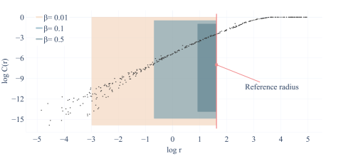
((a))

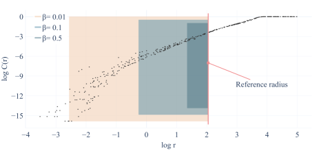
((b))

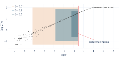
((c))

Figure 2: Log-log plot of correlation sums versus the radius used to estimate the correlation dimension for Lorenz (2(a)), Rössler (2(b)) and Hénon (2(c)) systems. The dots correspond to estimates of the correlation sum at random values of radius for trajectories integrated from random initial states. The colored regions show different ranges defined by $\left[\beta r_{\text{opt}},r_{\text{opt}}\right]$, with $\beta=0.01$ (in beige), $0.1$ (in light blue) or $0.5$ (in dark blue).

On 2(b), a knee is present around a value $\log(r_{\text{knee}})\simeq-1$, such that the slope $a_{\text{left}}$ in a left range $[r_{0},r_{\text{knee}}]$ is higher than the slope $a_{\text{right}}$ in right range $[r_{\text{knee}},r_{1}]$. In practice, a knee may appear from the superposition of signals from non-interacting subsystems with different amplitude (Eckmann and Ruelle, 1985). In this situation, $a_{\text{left}}$ characterizes the two subsystems while $a_{\text{right}}$ corresponds only to the system with the largest signal amplitude. Consequently, a careful analysis of the plot of $\log C(r,n)$ vs $\log r$ might be necessary to select a range capturing the desired properties of systems under study.

5.4 Influence of the time series length

Using the procedure described in Section 5.2, we generate $100$ trajectories for each length:

1. $N=250,500,1000,2500,5000$ for the Lorenz system,

2. $N=500,1000,2500,5000,7500$ for the Rössler system,

3. $N=100,250,500,1000,2500$ for the Hénon map.

Remark 3.

Notice that the discrepancies for the number of points used for the three systems can be justified by the resulting trajectories after time delay embedding. Indeed, when the number of points is too low, the reconstructed trajectories cannot properly reflect the dynamics nor the correct dimension of the attractor. For instance, in our experiments this was the case for time series of 100 points for the Rössler system.

We computed correlations sums for $20$ values of $r$ ranging between $10^{-8}$ and $2\sigma$, where $\sigma$ is the sample standard deviation. We compared the estimation using the Grassberger and Proccacia algorithm on the entire curve (the plateau on the right was omitted) with the estimation for $20$ values of $r$ in the meaningful range $(\beta r_{\text{opt}},r_{\text{opt}})$, for values of $\beta\in\{0.01,0.1,0.5\}$. We show in Figure 3 a violin plot of the estimated values depending on the duration of the time series and the range used to estimate the dimension. We compare our estimations with the values of correlation dimension reported by Sprott and Rowlands (Sprott and Rowlands, 2001) for much longer series ($2.049\pm 0.096$ for Lorenz attractor, $1.986\pm 0.078$ for Rössler attractor, $1.220\pm 0.036$ for Hénon map).

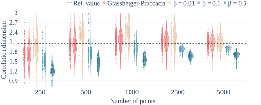
((a))

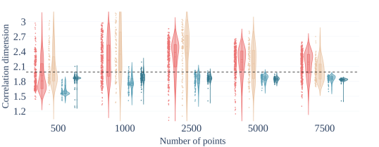
((b))

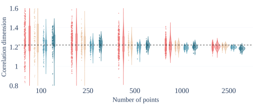
((c))

Figure 3: Influence of the number of points on the estimation of the correlation dimension from Lorenz (3(a)), Rössler (3(b)) and Hénon (3(c)) systems. We compare the original version of the Grassberger and Proccacia algorithm (red) with an estimation of the slope in the range $\left[\beta r_{\text{opt}},r_{\text{opt}}\right]$, with $\beta=0.01$ (beige), $\beta=0.1$ (light blue), $\beta=0.5$ (dark blue).

Overall, we observe that the spread of the estimations decreases with increasing $\beta$. With $\beta=0.01$ (beige) the result is almost similar to the original version of the Grassberger and Proccacia algorithm (red). In contrast, estimations for larger values of $\beta$ are more localized, but around values of dimension further apart from the reference dimension. We observe that the number of points affects significantly the variance of the estimations for larger values of $\beta$. However, for both Rössler and Hénon attractors, the range parameter $\beta=0.1$ (light blue) gives estimations with lower variance and bias compared to $\beta=0.5$ (dark blue). This suggests that the range must be selected sufficiently large to provide a proper support for dimension estimation. Moreover, although the bias of the Grassberger-Proccacia algorithm is low in this setup, a single dimension estimate can be far from the true dimension. Therefore, one can favor a smaller range for $r$ to reliably estimate a quantity slightly lower than the true dimension.

We found qualitatively similar results for Lorenz and Rössler attractors when series of different length are obtained by downsampling an original series of fixed length (results not shown).

5.5 Influence of observational white noise

Finally, we investigate the influence of observational noise on the estimation of the correlation dimension in the different ranges. Observational noise is ubiquitous in practical applications and creates a knee on the plot of $\log C(r,n)$ versus $\log r$, with a dimension at the left of the knee equal to the embedding dimension (see (Eckmann and Ruelle, 1985; Grassberger and Procaccia, 2004)). Hence, the range must be selected at the right of the knee to provide good estimations of the dimension.

We generate 100 time series of 1000 points for the three systems. Each series, with standard deviation $\sigma$, is corrupted with additive white Gaussian noise with standard deviation $\sigma_{\text{noise}}=k\,\sigma$, where $k$ defines the noise level. As above, we compare the estimation of the original Grassberger and Proccacia algorithm with the estimation in the different ranges (the reference radius (14) is computed for each noise-corrupted series). We present in Figure 4 a violin plot for noise levels $k=0,0.05,0.1,0.15,0.2$. For both Rössler and Lorenz attractors, we observe that a noise level of 5% is sufficient to corrupt estimations with the original version of the Grassberger and Proccacia algorithm (red) or the range $\beta=0.01$ (beige). In contrast, larger values of $\beta$ yield more consistent results under the different noise conditions. Therefore, this observation suggests that in noise conditions, the correlation dimension can be more robustly estimated from a smaller range of $r$.

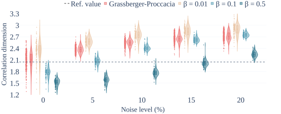
((a))

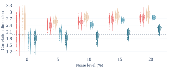
((b))

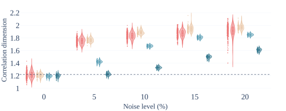
((c))

Figure 4: Estimation of the correlation dimension from Lorenz (4(a)), Rössler (4(b)) and Hénon (4(c)) systems under different levels of additive white Gaussian noise: comparison of the original Grassberger and Proccacia algorithm (blue) with an estimation of the slope in the range $\left[\beta r_{\text{opt}},r_{\text{opt}}\right]$, with $\beta=0.01$ (beige), $\beta=0.1$ (light blue), $\beta=0.5$ (dark blue).

6 Estimation of Kolmogorov-Sinai entropy using recurrence plots

In this section, we investigate the behavior of the goodness-of-fit of an estimator of a nonlinear measure with the radius parameter. We also study the reference radius inherent to (14) under different conditions. We use the reference radius in the construction of recurrence plots used to estimate the Kolmogorov-Sinai (KS) entropy of Hénon map and apply similar method to real electroencephalographic (EEG) signals.

6.1 Recurrence plots and Kolmogorov-Sinai entropy

6.1.1 Recurrence plots

Recurrence plots (Eckmann et al., 1987) display phase-space neighbors as a 2D black-and-white image whose $(i,j)$ element is black if trajectory points $x_{i}$ and $x_{j}$ are closer than a fixed radius $\varepsilon$. More formally, from a phase-space trajectory $\{x_{i}\},1\leq i\leq n$, a recurrence plot $\textsc{rp}(\varepsilon)\in\mathbb{R}^{n\times n}$ is defined as:

$$(\textsc{rp}(\varepsilon))_{i,j}=\Theta(\varepsilon-\|x_{i}-x_{j}\|_{p})$$ (23)

where $\Theta(\cdot)$ denotes Heaviside step function, $\|\cdot\|_{p}$ is a norm, usually either $L_{1}$, $L_{2}$, or $L_{\infty}$. The patterns in recurrence plots reflect properties of the underlying dynamical system and can be quantified using the Recurrence Quantification Analysis (RQA) framework, providing a set of powerful non-parametric visualization and characterization tools for nonlinear time series analysis. The relationship between recurrence plots (and RQA measures) and the correlation sum intuitively follows (23) (Grendár et al., 2013). Indeed, simple mathematical manipulations show that the recurrence rate, defined as the average number of recurrent points in a recurrence plot, is equal to the correlation sum (Thiel et al., 2003).

6.1.2 Estimating Kolmogorov-Sinai entropy from recurrence plots

The Kolmogorov-Sinai (KS) or measure-theoretic entropy (Kolmogorov, 1985; Sinai Ya, 1959) measures the evolution of uncertainty with the iteration of the map of a dynamical system. The lower bound $K_{2}$, often used as the estimate of KS entropy (Faure and Korn, 1998), is defined as (Grassberger and Procaccia, 1983b):

$$K_{2}=\lim\limits_{r\to 0}\lim\limits_{m\to\infty}\lim\limits_{n\to\infty}\frac{1}{\Delta t}\log\dfrac{C^{m}(r,n)}{C^{m+1}(r,n)}$$ (24)

$C^{m}(r,n)$ denotes the correlation sum built from a delay-reconstructed trajectory in a $m$-dimensional $L_{\infty}$ space. While it is possible to approximate the KS entropy directly from correlation sums (Pincus, 1991; Richman and Moorman, 2000), we rather consider the method in (Faure and Korn, 1998). The latter approximates the KS entropy from the histogram of diagonal lines of length greater than $m$ in a recurrence plot $\textsc{rp}(\varepsilon)$:

$$N^{\varepsilon}(m)=\text{card}\{(i,j):\forall k\in\{0,\dots,m-1\},|u_{i+k}-u_{j+k}|<\varepsilon\}$$ (25)

A diagonal of size $m$ on a recurrence plot reflects that two trajectories stayed at a distance smaller than a threshold $\varepsilon$ for $m$ time-steps, or equivalently that two delay-reconstructed vectors in $m$-dimensional space are close under $L_{\infty}$ norm. Hence, the histogram of diagonal lines, $N^{\varepsilon}(m)$, captures information similar to the correlation sum from delay-coordinates, $C^{m}(r,n)$; whereas the parameters $\varepsilon$ and $r$ are analogous in the two quantities. The main advantage of the Faure and Korn method is computational: while $C^{m}(r,n)$ is computed for several values of the embedding dimension $m$, the histogram $N^{\varepsilon}(m)$ is computed only once. Then, using the diagonal line histograms to rewrite the KS entropy (24) as a function of $r=\varepsilon$ gives:

$$K_{2}(r)=\lim\limits_{m\to\infty}\lim\limits_{n\to\infty}\frac{1}{\Delta t}\log\dfrac{N^{r}(m+1)}{N^{r}(m+2)}$$ (26)

Faure and Korn (Faure and Korn, 1998) suggest to evaluate the average slope of a $\log N^{r}(m)$ vs $m$ plot for various values of $r$. Then, taking the limit $r\to 0$ is supposed to converge to a constant value equal to the KS entropy, $K_{2}$, up to a scaling factor. However, selecting the smallest possible $r$ to estimate the limit $r\to 0$ from real-world data (i.e. finite-size samples with noise) likely leads to estimations flawed by a large variance, as discussed in (Faure and Lesne, 2015). Hence, the problem is to select a value of $r$ yielding the best possible estimations of the KS entropy. We use our reference radius ((14)) to compute the recurrence plot used to estimate the KS entropy. Recurrence plots and diagonal line histograms were computed using the pyunicorn package (Donges et al., 2015).

6.2 Numerical experiments for the Hénon map

We generate 100 time series for each length ($n=150,250,500,1500$ points) from the standard Hénon map ($a=1.4$, $b=0.3$). For each series, we use the Faure and Korn method and compute the value of $K_{2}(r)$, (26), as a function $\log r$ curve for $50$ values of $\log r$ ranging from $-4$ to $0.5$. We then compute the reference radius ((14)) — using the series length $n$ and dimension $d=1$ — and average the values over series of same length. Results are presented in Figure 5.

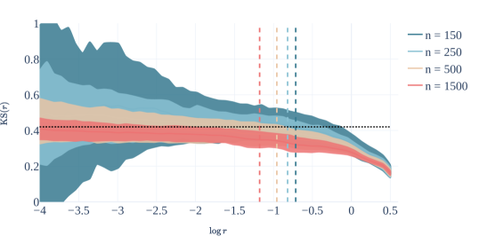
Figure 5: Estimation of Kolmogorov-Sinai entropy for time series from the Hénon map with different lengths $n$. The filled areas corresponds to the $95\%$ (Gaussian) confidence intervals for each length. The vertical dashed lines represents the average reference radius associated to each length. The horizontal dashed line indicates the reported entropy for Hénon map, $K_{2}=0.42$.

We notice that the variance of the estimation increases for decreasing radius and decreasing number of points. This result is presumably due to a poor statistical power for small values of the radius and short time series. However, the estimation seems to converge in average to the theoretical value ($H_{KS}=0.42$ (Faure and Korn, 1998)) when $r$ tends to $0$. Notice that the right-most part of the plot exhibits a large bias between the estimated and theoretical entropy values. Contrary to the variance, the bias does not seem to decrease with increasing number of points. Thus this bias is more symptomatic of the radius being too high to obtain any valuable information about the Hénon map. This bias-variance trade-off is usually related to a Mean Squared Error (MSE) minimization problem.

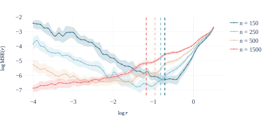
Figure 6: Estimation of the log-Mean Square Error of the Kolmogorov-Sinai entropy estimator as a function of the radius value (lower is better). The filled areas corresponds to the $95\%$ bootstrap confidence interval for each length. We see that for different time series, the reference radius gives a log-MSE value between $-7$ and $-5$.

As the MSE of an estimator quantifies the goodness-of-fit, the parameters of the estimator yielding the minimum value of MSE can be systematically selected. We numerically compute the MSE of the KS entropy estimator as a function of $\log r$ and use this plot as an objective criterion to evaluate the adequacy of our reference radius. The MSE consists in the sum of a squared bias term, measuring the difference between the theoretical value and the estimation, as well as the variance of the estimator. We use a theoretical value $K_{2}=0.42$ and all of the 100 sample series to compute the MSE, overlay the reference radius averaged over series of same length, and show the results in Figure 6. For short time series, we observe that the radius selected by the reference rule is systematically close to the minimum of the MSE. For longer time series, the reference radius is larger than the minimum of the curve. Nevertheless, for values of $r<r_{\text{opt}}$, the slope of the MSE curve gets flatter for increasing number of points and allows arbitrary selection of smaller radius values. We report similar observations for two other estimators of the KS entropy, the Approximate and Sample entropies (results not shown).

6.3 Application to EEG signals in the context of epilepsy

To show the viability of our approach on real-world data, we apply our radius selection procedure to estimate the KS entropy of epileptic EEG signals. A significant decrease of the EEG signal entropy at the epileptic seizure location is a common feature for automatic seizure detection (Ocak, 2008; Srinivasan et al., 2007). We use the data publicly available from the University of Bonn (Andrzejak et al., 2001), which consists in five sets of EEG data. Each set contains 100 segments of $23.6$ seconds recorded at $173.61$Hz (4096 points per segment), which were visually inspected for artifacts and band-pass filtered between $0.5$Hz and $40$Hz. Two sets contains surface EEG recorded from five healthy volunteers at rest, either with closed (set O) and opened eyes (set Z). The three other sets, consisting in signals from five epileptic patients recorded during presurgical evaluation, contain segments either from seizure-free intervals (at epileptogenic site, set F, or at the hippocampal formation of the opposite hemisphere of the brain, set N) or during seizure (at epileptogenic site, set S).

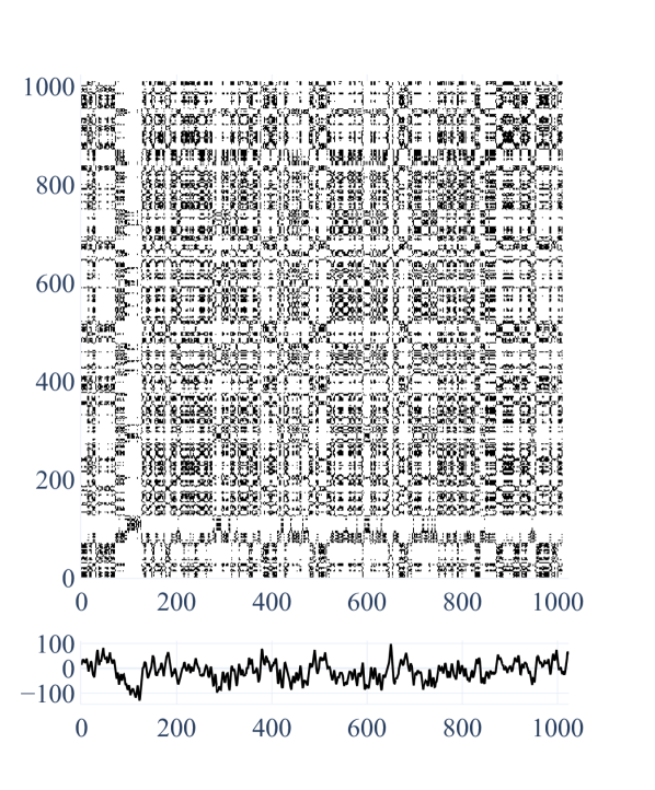
((a))

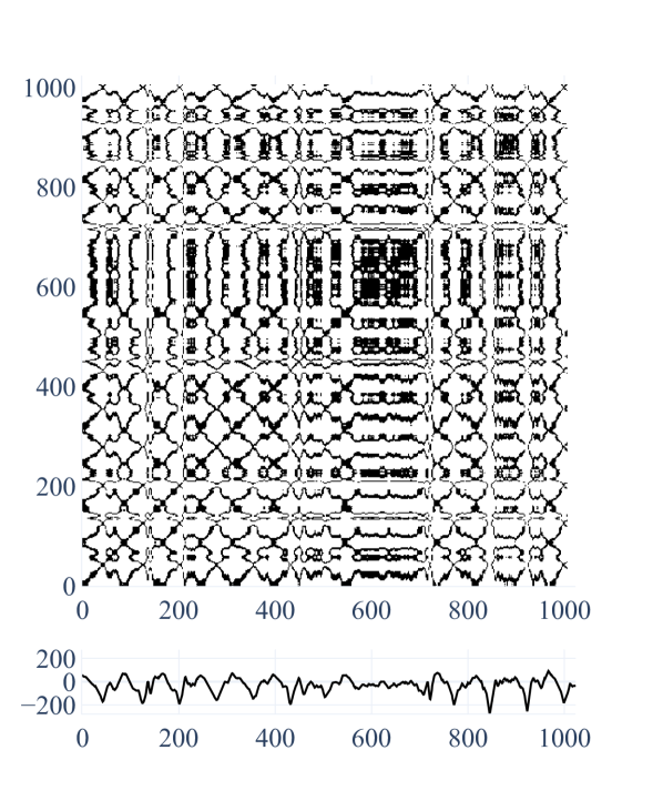
((b))

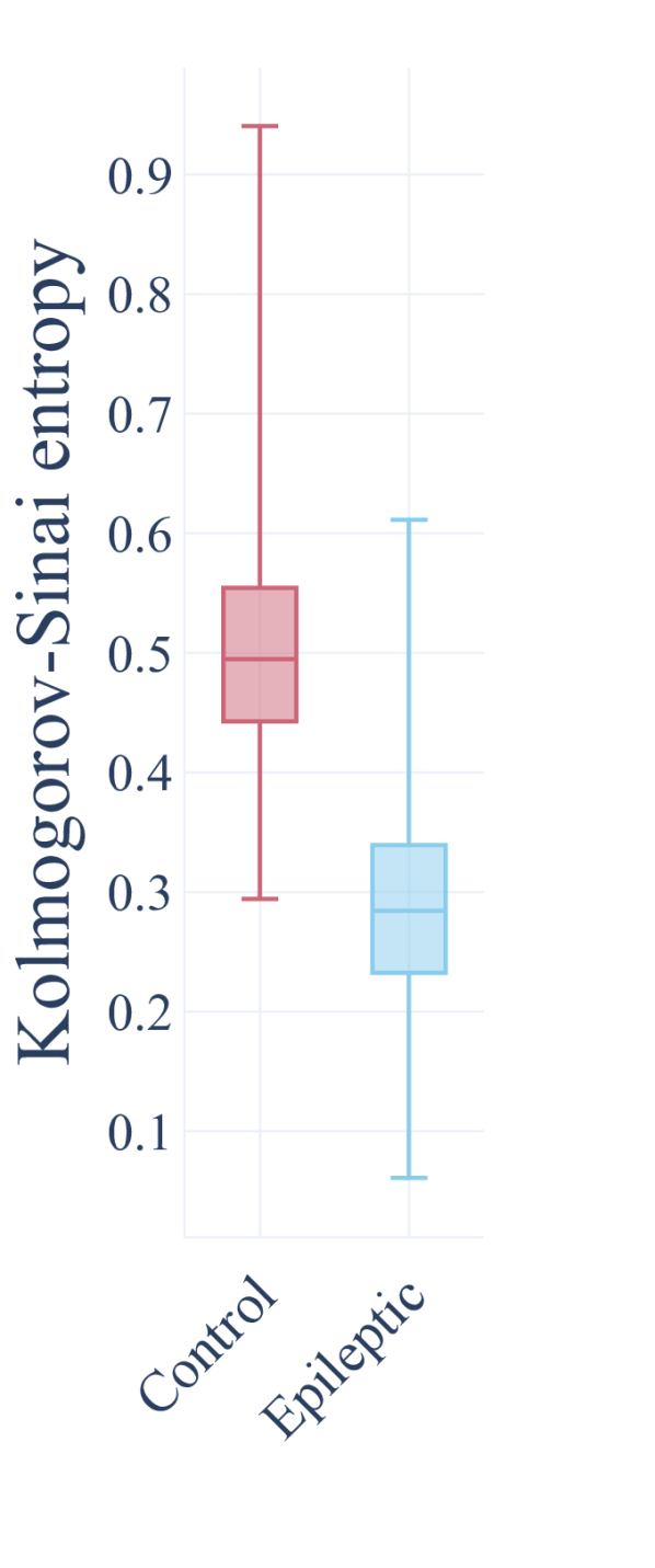
((c))

Figure 7: Estimation of the Kolmogorov-Sinai entropy from recurrence plots to discriminate epileptic from healthy EEG signals: (7(a)) and (7(b)) show sample EEG signals and recurrence plots for an healthy volunteer and an epileptic patient respectively. The value $r=1.843\times\hat{s}\times n^{-1/5}$ ((14)) is used to compute the recurrence plots from the univariate time series; (7(c)) contains a box plot of the estimated entropies for both control and epileptic groups. As expected, the entropy values are significantly lower for the epileptic group.

Each record is divided in four segments of 1024 points. For each segment, we compute a recurrence plot with the radius set by (14) and estimate the KS entropy using the Faure and Korn method. Recurrence plots and signals sampled from the sets Z and F are shown in 7(a) and 7(b). We present in 7(c) a box plot of the KS entropy for the healthy volunteers (control group) and the epileptic patients. Our estimator gives an average KS entropy of $0.288\pm 0.005$ (95% confidence interval) for the epileptic group and $0.504\pm 0.006$ for the control group, which confirms an average significant decrease of the KS entropy with epilepsy, as reported in previous studies (Kannathal et al., 2005).

Finally, to compare the discrimination strength of common closed-form radius selection methods, we estimate the KS entropy with each method, perform a two-samples Z-test (epileptic versus control group) and collect the Z-score. We report a Z-score of $Z=45.3$ (resp. $Z=39.3$) for the $r=0.2\sigma$ (resp. $r=0.1\sigma$, with $\sigma$ the series standard deviation) rule (Pincus, 1991), $Z=48.9$ when the radius is set to $10\%$ of the maximum phase space neighborhood (Zbilut and Webber Jr, 1992), $Z=41.1$ (resp. $Z=34.6$) when the radius is selected such that $10\%$ (resp. $4$%) of the number of points are selected as neighbors (Webber and Marwan, 2015; Kraemer et al., 2018), $Z=54.9$ for the reference rule radius $r=1.843\times\hat{s}\times n^{-1/5}$ ((14)). Subsequently, although all methods detect significant differences between the two groups, the radius given by (14) gives the most statistically significant results.

7 Discussion and conclusion

We propose a new approach for selecting the radius parameter in nonlinear measures derived from the correlation sum. We first formulate a relative error function on the quantities underlying correlation sums. We show that minimizing the loss function is equivalent to minimizing the MISE of a kernel density estimator. We use the AMISE minimization method to derive a closed-form expression to select the radius. Additionally, we observe how the bias and variance of the estimator varies with the radius and derive a “meaningful” range to select a variable radius.

We investigate the behavior of the Grassberger and Proccacia algorithm for estimating the correlation dimension in radius ranges of different size. We observe that the range parameter $\beta$ can be selected close to $1$ for low-variance estimations, and close to $0$ for low-bias estimations. However, the presence of noise in the observed signal induces typical error in the estimations and leads to favor small ranges close to the reference radius.

We then use the reference radius to construct recurrence plots for estimating the Kolmogorov-Sinai entropy from both simulated and experimental signals. In a first analysis, we reconstruct the Mean Squared Error curve of the entropy estimator for Hénon map and show that the reference radius is close to the minimum of the curve. We confirm the experimental adequacy of the method by obtaining significant results in characterizing epileptic EEG signals.

Moreover, our theoretical approach yields a reference radius that is similar to several existing radius selection methods arising from empirical or numerical experience: the radius is a fraction of the scale of the data (Pincus, 1991; Zbilut and Webber Jr, 1992) and compensates for the dimension of the data (Kraemer et al., 2018).

For the specific case of recurrence plots, (Andreadis et al., 2020) recently proposed an empirical procedure to identify an optimal radius value. They define a metric to measure the distance between recurrence plots and compute the distance between recurrence plots constructed from the same time series using increasing values of radius. The radius value is considered “optimal” when it minimizes the distance between consecutive recurrence plots, i.e. such that a slightly changing the radius has the minimal impact on the recurrence plot. The principal issues with this procedure are the computational burden of building several recurrence plots and the difficulty to reliably identify the optimum. In contrast, our method is computationally much more efficient and not restricted to recurrence plots.

Our numerical experiments suggest that the reference radius given in (14) can be used as a default parameter to obtain robust and significant values for a number of different nonlinear tools and measures: correlation dimension, recurrence plots, Kolmogorov-Sinai entropy. In future work, we plan to investigate the relation between our optimal radius and the embedding parameters, which play a role on the trajectories resolution in the reconstructed phase space. Additionally, we plan to use the reference radius in EEG signal processing application, notably to extract dynamical features characterizing the oscillatory dynamics of motor imagery EEG signals.

Appendix A Volume of generalized balls

Let $B_{r}^{p,d}(x)$ be an open $d$-ball of size $r$ in an $L_{p}$ space, i.e. $B_{r}^{p,d}(x)=\{y\in\mathbb{R}^{d}:\|x-y\|_{p}<r\}$. We write $\tau_{p,d}=\lambda(B_{1}^{p,d})$ the volume of the generalized unit ball, where $\lambda$ is the Lebesgue measure. The volume of a generalized ball of radius $r$ is $\lambda(B_{r}^{p,d})=\tau_{p,d}r^{d}$. The general formula for the volume of a generalized unit ball is (Wang, 2005):

$$\tau_{p,d}=\frac{(2\Gamma(\frac{1}{p}+1))^{d}}{\Gamma(\frac{d}{p}+1)}$$ (27)

which can be simplified for common $L_{p}$ spaces:

$$\tau_{1,d} =\frac{2^{d}}{d!} \tau_{2,d} =\frac{\pi^{\frac{d}{2}}}{\Gamma(\frac{d}{2}+1)} \tau_{\infty,d} =2^{d}$$ (28)

$\Gamma$ denotes Euler’s gamma function with the property $\Gamma(z+1)=z\Gamma(z)$.

Appendix B Derivation of a reference rule for the uniform kernel

The expression of the bandwidth minimizing the Asymptotic Mean Integrated Squared Error is ((Silverman, 1986), Eq. 4.14 and 4.15):

$$h_{\text{AMISE}}=\left[\dfrac{W_{1}(K)\cdot d}{n\cdot\left[W_{2}(K)\right]^{2}\cdot W_{1}(\nabla^{2}f)}\right]^{1/(d+4)}$$ (29)

where $W_{i}$ are the functionals $W_{1}(g)=\int_{\mathbb{R}^{d}}g^{2}(u)du$ and $W_{2}(g)=\int_{\mathbb{R}^{d}}u_{1}^{2}g(u)du$, where $u_{1}$ is the first component of $u\in\mathbb{R}^{d}$ (as the kernel is symmetric, it is sufficient to consider only $u_{1}$ in $W_{2}$). We compute $W_{1}$ for the uniform kernel:

$$W_{1}(K)=\int\limits_{\mathbb{R}^{d}}K^{2}(u)du=\int\limits_{B_{1}^{p,d}(0)}\left(\frac{1}{\tau_{p,d}}\right)^{2}du=\frac{1}{\tau_{p,d}}$$ (30)

$W_{1}(\nabla^{2}\rho)$ for a $d$-dimensional Gaussian reference distribution $\phi$ is given in (Silverman, 1986, Eq. 4.13):

$$W_{1}(\nabla^{2}\rho)\approx W_{1}(\nabla^{2}\phi)=(2\sqrt{\pi})^{-d}\left(d/2+d^{2}/4\right)$$ (31)

Then, $W_{2}$ in the 1-dimensional case:

$$W_{2}(K)=\int\limits_{\mathbb{R}}u^{2}K(u)du=\int\limits_{-1}^{1}\frac{u^{2}}{\tau_{p,1}}du=\frac{1}{3}$$ (32)

For $d\geq 2$, using $u_{i}$ to denote the $i$-th coordinate of $u\in\mathbb{R}^{d}$:

$$W_{2}(K) =\int\limits_{\mathbb{R}^{d}}u_{1}^{2}K(u)du$$

$$=\frac{1}{\tau_{p,d}}\int\limits_{\mathbb{R}}u_{1}^{2}\left(\,\,\int\limits_{\mathbb{R}^{d-1}}\Theta(1-(|u_{1}|^{p}+\sum_{i=2}^{d}|u_{i}|^{p})^{1/p})du_{d}\dots du_{2}\right)\,du_{1}$$

Changing to spherical coordinates $\vec{u}_{2:d}=(\eta,\vec{\xi})$ with an orientation vector $\vec{\xi}$ and a radius $\eta=(\sum_{i=2}^{d}|u_{i}|^{p})^{1/p}$ and :

$$W_{2}(K) =\frac{1}{\tau_{p,d}}\int\limits_{\mathbb{R}}u_{1}^{2}\int\limits_{\eta=0}^{\infty}\int\limits_{\mathbb{R}^{d-2}}\Theta\left(1-(|u_{1}|^{p}+\eta^{p})^{1/p}\right)d\vec{\xi}\,d\eta\,du_{1}$$

$$=\frac{\tau_{p,d-1}}{\tau_{p,d}}\int\limits_{\mathbb{R}}u_{1}^{2}\int\limits_{\eta=0}^{\infty}(d-1)\eta^{d-2}\Theta\left(1-(|u_{1}|^{p}+\eta^{p})^{1/p}\right)d\eta\,du_{1}$$

$$=\frac{\tau_{p,d-1}}{\tau_{p,d}}\int\limits_{u_{1}=-1}^{1}u_{1}^{2}\int\limits_{\eta=0}^{(1-|u_{1}|^{p})^{1/p}}{(d-1)}\eta^{d-2}d\eta\,du_{1}$$

$$=\frac{\tau_{p,d-1}}{\tau_{p,d}}\int\limits_{u_{1}=-1}^{1}u_{1}^{2}\left((1-|u_{1}|^{p})^{1/p}\right)^{(d-1)}\,du_{1}$$

$$=\frac{\tau_{p,d-1}}{\tau_{p,d}}\frac{2}{3}{}_{2}F_{1}\left(\frac{3}{p},\frac{1-d}{p};\frac{3+p}{p};1\right)$$

where ${}_{2}F_{1}(a,b;c;z)$ is the Gaussian hypergeometric function. Finally, using the fact that $\frac{\tau_{p,d-1}}{\tau_{p,d}}=\frac{\Gamma(\frac{d}{p}+1)}{2\Gamma(\frac{1}{p}+1)\Gamma(\frac{d-1}{p}+1)}$, (see Appendix A.1) and the expansion of ${}_{2}F_{1}$ at $z=1$ (Olver et al., 2020, Eq. 15.4.20), we can further simplify:

$$W_{2}(K) =\frac{\tau_{p,d-1}}{\tau_{p,d}}\frac{2\Gamma\left(1+\frac{3}{p}\right)\Gamma\left(\frac{d-1}{p}+1\right)}{3\Gamma\left(\frac{d+2}{p}+1\right)}=\frac{\Gamma\left(\frac{d}{p}+1\right)\Gamma\left(1+\frac{3}{p}\right)}{3\Gamma\left(\frac{d+2}{p}+1\right)\Gamma\left(\frac{1}{p}+1\right)}$$ (33)

We then derive the reference rule by plugging the appropriate values in (29). First, we derive the expression in the simple 1 dimensional case, which is independent from $p$:

$$r_{\text{opt}}=\left[12\sqrt{\pi}\right]^{1/5}\cdot\hat{s}\cdot n^{-1/5}\approx 1.843\cdot\hat{s}\cdot n^{-1/5}$$ (34)

The general formula for $d\geq 2$ is more complex:

$$r_{\text{opt}} =\left[\dfrac{4d(2\sqrt{\pi})^{2}}{\tau_{p,d}d(d+2)}\times\dfrac{\left(3\Gamma\left(\frac{d+2}{p}+1\right)\Gamma\left(\frac{1}{p}+1\right)\right)^{2}}{\left(\Gamma\left(\frac{d}{p}+1\right)\Gamma\left(1+\frac{3}{p}\right)\right)^{2}}\right]^{1/(d+4)}\cdot\hat{s}\cdot n^{-1/(d+4)}$$

$$=\left[\dfrac{4(2\sqrt{\pi})^{d}\left(3\Gamma\left(\frac{d+2}{p}+1\right)\Gamma\left(\frac{1}{p}+1\right)\right)^{2}}{\tau_{p,d}(d+2)\left(\Gamma\left(\frac{d}{p}+1\right)\Gamma\left(1+\frac{3}{p}\right)\right)^{2}}\right]^{1/(d+4)}\cdot\hat{s}\cdot n^{-1/(d+4)}$$ (35)

Appendix C Simplification of the reference rule for common norms

We address the case $p=1$:

$$r_{\text{opt}} =\left[\dfrac{4(2\sqrt{\pi})^{d}\left(3\Gamma\left(d+3\right)\Gamma\left(2\right)\right)^{2}}{\tau_{p,d}(d+2)\left(\Gamma\left(d+1\right)\Gamma\left(4\right)\right)^{2}}\right]^{1/(d+4)}\cdot\hat{s}\cdot n^{-1/(d+4)}$$

$$=\left((\sqrt{\pi})^{d}(d+1)\left(d+2\right)!\right)^{1/(d+4)}\cdot\hat{s}\cdot n^{-1/(d+4)}$$ (36)

Then, the limiting case $p\to\infty$:

$$r_{\text{opt}} =\left[\dfrac{4(2\sqrt{\pi})^{d}\left(3\Gamma\left(1\right)\Gamma\left(1\right)\right)^{2}}{\tau_{p,d}(d+2)\left(\Gamma\left(1\right)\Gamma\left(1\right)\right)^{2}}\right]^{1/(d+4)}\cdot\hat{s}\cdot n^{-1/(d+4)}$$

$$=\left[\frac{36(\sqrt{\pi})^{d}}{d+2}\right]^{1/(d+4)}\cdot\hat{s}\cdot n^{-1/(d+4)}$$ (37)

Finally the case $p=2$:

$$r_{\text{opt}} =\left[\dfrac{4(2\sqrt{\pi})^{d}\left(3\Gamma\left(\frac{d+2}{2}+1\right)\Gamma\left(\frac{1}{2}+1\right)\right)^{2}}{\tau_{2,d}(d+2)\left(\Gamma\left(\frac{d}{2}+1\right)\Gamma\left(1+\frac{3}{2}\right)\right)^{2}}\right]^{1/(d+4)}\cdot\hat{s}\cdot n^{-1/(d+4)}$$

$$=\left[\dfrac{2^{d+2}\Gamma\left(\frac{d}{2}+1\right)\left(3\Gamma\left(\frac{d}{2}+1\right)(\frac{d}{2}+1)\Gamma\left(\frac{1}{2}+1\right)\right)^{2}}{(d+2)\left(\Gamma\left(\frac{d}{2}+1\right)\Gamma\left(1+\frac{1}{2}\right)(1+\frac{1}{2})\right)^{2}}\right]^{1/(d+4)}\cdot\hat{s}\cdot n^{-1/(d+4)}$$

$$=\left[2^{d+2}\Gamma\left(\frac{d}{2}+1\right)(d+2)\right]^{1/(d+4)}\cdot\hat{s}\cdot n^{-1/(d+4)}$$

$$=2\left[\frac{\Gamma\left(\frac{d}{2}+1\right)}{2}\right]^{1/(d+4)}\cdot\hat{s}\cdot n^{-1/(d+4)}$$ (38)

References

- Andreadis et al. (2020) Andreadis, I., Fragkou, A. D. and Karakasidis, T. E. (2020) On a topological criterion to select a recurrence threshold. Chaos: An Interdisciplinary Journal of Nonlinear Science, 30, 013124.
- Andrzejak et al. (2001) Andrzejak, R. G., Lehnertz, K., Mormann, F., Rieke, C., David, P. and Elger, C. E. (2001) Indications of nonlinear deterministic and finite-dimensional structures in time series of brain electrical activity: Dependence on recording region and brain state. Physical Review E, 64, 061907.
- Donges et al. (2015) Donges, J. F., Heitzig, J., Beronov, B., Wiedermann, M., Runge, J., Feng, Q. Y., Tupikina, L., Stolbova, V., Donner, R. V., Marwan, N. et al. (2015) Unified functional network and nonlinear time series analysis for complex systems science: The pyunicorn package. Chaos: An Interdisciplinary Journal of Nonlinear Science, 25, 113101.
- Eckmann et al. (1987) Eckmann, J.-P., Kamphorst, S. O. and Ruelle, D. (1987) Recurrence plots of dynamical systems. EPL (Europhysics Letters), 4, 973.
- Eckmann and Ruelle (1985) Eckmann, J.-P. and Ruelle, D. (1985) Ergodic theory of chaos and strange attractors. In The theory of chaotic attractors, 273–312. Springer.
- Erdogmus and Principe (2006) Erdogmus, D. and Principe, J. C. (2006) From linear adaptive filtering to nonlinear information processing-the design and analysis of information processing systems. IEEE Signal Processing Magazine, 23, 14–33.
- Faure and Korn (1998) Faure, P. and Korn, H. (1998) A new method to estimate the Kolmogorov entropy from recurrence plots: its application to neuronal signals. Physica D: Nonlinear Phenomena, 122, 265–279.
- Faure and Korn (2001) — (2001) Is there chaos in the brain? I. Concepts of nonlinear dynamics and methods of investigation. Comptes Rendus de l’Académie des Sciences-Series III-Sciences de la Vie, 324, 773–793.
- Faure and Lesne (2015) Faure, P. and Lesne, A. (2015) Estimating Kolmogorov entropy from recurrence plots. In Recurrence Quantification Analysis, 45–63. Springer.
- Fraser and Swinney (1986) Fraser, A. M. and Swinney, H. L. (1986) Independent coordinates for strange attractors from mutual information. Physical review A, 33, 1134.
- Freeman (2003) Freeman, W. J. (2003) Evidence from human scalp electroencephalograms of global chaotic itinerancy. Chaos: An Interdisciplinary Journal of Nonlinear Science, 13, 1067–1077.
- Ghil et al. (2008) Ghil, M., Chekroun, M. D. and Simonnet, E. (2008) Climate dynamics and fluid mechanics: Natural variability and related uncertainties. Physica D: Nonlinear Phenomena, 237, 2111–2126.
- Grassberger and Procaccia (1983a) Grassberger, P. and Procaccia, I. (1983a) Characterization of strange attractors. Physical review letters, 50, 346.
- Grassberger and Procaccia (1983b) — (1983b) Estimation of the Kolmogorov entropy from a chaotic signal. Physical review A, 28, 2591.
- Grassberger and Procaccia (2004) — (2004) Measuring the strangeness of strange attractors. In The theory of chaotic attractors, 170–189. Springer.
- Grendár et al. (2013) Grendár, M., Majerová, J. and Špitalskỳ, V. (2013) Strong laws for recurrence quantification analysis. International Journal of Bifurcation and Chaos, 23, 1350147.
- Gunduz and Principe (2009) Gunduz, A. and Principe, J. C. (2009) Correntropy as a novel measure for nonlinearity tests. Signal Processing, 89, 14–23.
- Hang et al. (2018) Hang, H., Steinwart, I., Feng, Y. and Suykens, J. A. (2018) Kernel density estimation for dynamical systems. The Journal of Machine Learning Research, 19, 1260–1308.
- Hénon (1976) Hénon, M. (1976) A two-dimensional mapping with a strange attractor. In The Theory of Chaotic Attractors, 94–102. Springer.
- Jones et al. (1996) Jones, M. C., Marron, J. S. and Sheather, S. J. (1996) A brief survey of bandwidth selection for density estimation. Journal of the American statistical association, 91, 401–407.
- Kannathal et al. (2005) Kannathal, N., Choo, M. L., Acharya, U. R. and Sadasivan, P. (2005) Entropies for detection of epilepsy in eeg. Computer methods and programs in biomedicine, 80, 187–194.
- Kantz and Schreiber (2004) Kantz, H. and Schreiber, T. (2004) Nonlinear time series analysis, vol. 7. Cambridge university press.
- Kolmogorov (1985) Kolmogorov, A. N. (1985) A new metric invariant of transitive dynamical systems and automorphisms of Lebesgue spaces. Trudy Matematicheskogo Instituta imeni VA Steklova, 169, 94–98.
- Kraemer et al. (2018) Kraemer, K. H., Donner, R. V., Heitzig, J. and Marwan, N. (2018) Recurrence threshold selection for obtaining robust recurrence characteristics in different embedding dimensions. Chaos: An Interdisciplinary Journal of Nonlinear Science, 28, 085720.
- Lorenz (1963) Lorenz, E. N. (1963) Deterministic nonperiodic flow. Journal of the atmospheric sciences, 20, 130–141.
- Marwan et al. (2007) Marwan, N., Romano, M. C., Thiel, M. and Kurths, J. (2007) Recurrence plots for the analysis of complex systems. Physics reports, 438, 237–329.
- Moon et al. (1995) Moon, Y.-I., Rajagopalan, B. and Lall, U. (1995) Estimation of mutual information using kernel density estimators. Phys. Rev. E, 52, 2318–2321.
- Ocak (2008) Ocak, H. (2008) Optimal classification of epileptic seizures in EEG using wavelet analysis and genetic algorithm. Signal processing, 88, 1858–1867.
- Olver et al. (2020) Olver, F. W. J., Daalhuis, A. B. O., Lozier, D. W., Schneider, B. I., Boisvert, R. F., Clark, C. W., B. R. Mille and, B. V. S., Cohl, H. S. and M. A. McClain, e. (2020) Nist Digital Library of Mathematical Functions. http://dlmf.nist.gov/, Release 1.1.0 of 2020-12-15. URL: http://dlmf.nist.gov/.
- Ott (2002) Ott, E. (2002) Chaos in dynamical systems. Cambridge university press.
- Pesin (2008) Pesin, Y. B. (2008) Dimension theory in dynamical systems: contemporary views and applications. University of Chicago Press.
- Pincus (1991) Pincus, S. M. (1991) Approximate entropy as a measure of system complexity. Proceedings of the National Academy of Sciences, 88, 2297–2301.
- Principe (2010) Principe, J. C. (2010) Information theoretic learning: Renyi’s entropy and kernel perspectives. Springer Science & Business Media.
- Richman and Moorman (2000) Richman, J. S. and Moorman, J. R. (2000) Physiological time-series analysis using approximate entropy and sample entropy. American Journal of Physiology-Heart and Circulatory Physiology, 278, H2039–H2049.
- Rössler (1976) Rössler, O. E. (1976) An equation for continuous chaos. Physics Letters A, 57, 397–398.
- Scott (1979) Scott, D. W. (1979) On optimal and data-based histograms. Biometrika, 66, 605–610.
- Silverman (1986) Silverman, B. W. (1986) Density estimation for statistics and data analysis, vol. 26. CRC press.
- Sinai Ya (1959) Sinai Ya, G. (1959) On the notion of entropy of a dynamical system. In Doklady of Russian Academy of Sciences, vol. 124, 768–771.
- Singh and Príncipe (2011) Singh, A. and Príncipe, J. C. (2011) Information theoretic learning with adaptive kernels. Signal Processing, 91, 203–213.
- Sprott and Rowlands (2001) Sprott, J. C. and Rowlands, G. (2001) Improved correlation dimension calculation. International Journal of Bifurcation and Chaos, 11, 1865–1880.
- Srinivasan et al. (2007) Srinivasan, V., Eswaran, C. and Sriraam, N. (2007) Approximate entropy-based epileptic EEG detection using artificial neural networks. IEEE Transactions on information Technology in Biomedicine, 11, 288–295.
- Takens (1981) Takens, F. (1981) Detecting strange attractors in turbulence. In Dynamical systems and turbulence, Warwick 1980, 366–381. Springer.
- Thiel et al. (2003) Thiel, M., Romano, M. C. and Kurths, J. (2003) Analytical description of recurrence plots of white noise and chaotic processes. arXiv preprint nlin/0301027.
- Wang (2005) Wang, X. (2005) Volumes of generalized unit balls. Mathematics Magazine, 78, 390–395.
- Webber and Marwan (2015) Webber, C. and Marwan, N. (2015) Recurrence quantification analysis. Theory and Best Practices.
- Yang et al. (2018) Yang, Y.-X., Gao, Z.-K., Wang, X.-M., Li, Y.-L., Han, J.-W., Marwan, N. and Kurths, J. (2018) A recurrence quantification analysis-based channel-frequency convolutional neural network for emotion recognition from EEG. Chaos: An Interdisciplinary Journal of Nonlinear Science, 28, 085724.
- Yu et al. (2000) Yu, D., Small, M., Harrison, R. G. and Diks, C. (2000) Efficient implementation of the Gaussian kernel algorithm in estimating invariants and noise level from noisy time series data. Physical Review E, 61, 3750.
- Zbilut and Webber Jr (1992) Zbilut, J. P. and Webber Jr, C. L. (1992) Embeddings and delays as derived from quantification of recurrence plots. Physics letters A, 171, 199–203.