The Priced Survey Methodology: Theory

Abstract

In this paper, I introduce the Priced Survey Methodology (PSM), a tool designed to overcome the limitations of traditional survey methods in analyzing social preferences. The PSM’s design draws inspiration from consumption choice experiments, as respondents fill out the same survey multiple times under different choice sets. I generalize Afriat’s theorem and show that the Generalized Axiom of Revealed Preferences is necessary and sufficient for the existence of a concave, continuous, and single-peaked utility function rationalizing answers to the PSM. This result has two major implications. First, it is possible to measure a respondent’s ideal answer to a survey using only ordinal relations between possible answers. Second, the PSM captures aspects of social preferences often overlooked in standard surveys, such as the relative importance that respondents attribute to different survey questions. I deploy a PSM measuring altruistic preferences in a sample of online participants, recover respondents’ single-peaked preferences, and draw several implications.

JEL C9, D91, C44

Keywords: Decision Theory, Revealed Preference, Social Preferences, Behavioral Economics, Survey.

1 Introduction

One of the most fundamental contributions of economics to the history of thought is its ability to explain choices by a set of preferences. These preferences encompass consumption goods, attitudes towards risk, time, and social aspects. Specifically, social preferences include aspects such as altruism, identity, environmental concerns, political inclinations, and perceptions of fairness and justice, and are typically measured through specific experimental designs (e.g., Fehr and Schmidt (1999), Henrich et al. (2001), Abeler, Nosenzo and Raymond (2019)) or surveys (e.g., Desmet, Ortuño-Ortín and Wacziarg (2017), Falk et al. (2018), Stantcheva (2023)). While these two approaches are valuable in many contexts, they leave several points unanswered. To start, one common assumption behind experimental measures of social preferences is the existence of a utility representation that internalizes social aspects. However, little is known about the rationality axioms sustaining the existence of a utility representation for social preferences. As for surveys, there can be multiple decision mechanisms explaining survey answers. Moreover, individual survey data comparisons pose several challenges (Bond and Lang (2019)).

In this paper, I unveil the Priced Survey Methodology (PSM), a tool designed to overcome the limitations of traditional survey methods in analyzing social preferences. The PSM bridges the gap between decision theory and empirical survey data, enabling a more nuanced and precise exploration of how individuals form and express social preferences. The design of the PSM is close to experiments built to recover preferences from choices on linear budget sets as respondents fill the same survey multiple times under different choice sets. In every round of the PSM, each given participant initially sees a default answer. She can adjust this default to better match her preferences. However, adjusting the answer from the default is costly, and participants have a finite pool of credits in each round. The credit cost for deviations isn’t constant but varies between rounds. With this design, it is as if subjects were “buying” goods when they move from the default.

The first key contribution of this paper is theoretical. I generalize Afriat’s theorem and show that the Generalized Axiom of Revealed Preferences (GARP) is necessary and sufficient for the existence of a concave, continuous, and single-peaked utility function rationalizing answers to the PSM. Indeed, the default option in the PSM is not always the null answer, but is round-specific and necessarily belongs to a corner of the answer space. Consider for example a survey with two questions, both on a $\{0,\dots,10\}$ scale. In some rounds, the default might be $(10,10)$, so subjects might “pay” credits to decrease their answers, while in other rounds, the default might be $(0,0)$, in which case subjects pay to increase their answers to both questions. With this unique feature of the PSM design, it is possible to observe subjects revealing non-monotonic preferences.

The key intuition behind the Theorem is that it is possible to partition the space of possible answers $X$ into non-overlapping regions, $X=\bigcup_{c\in C(X)}r_{c}$, with $C(X)$ the set of corners in space $X$. Each region $r_{c}$ in that partition is comprehensive in the coordinate system originating in corner $c$. Moreover, to the extent that the PSM data satisfy GARP, then in any region $r_{c}$ of the partition, the utility function rationalizing the PSM data is continuous, concave, and monotonic in the coordinate system originating in corner $c$. The resulting utility - monotonic in each region in the coordinate system associated with that region - is single-peaked. Figure LABEL:fig_intro illustrates this intuition in the case of a PSM consisting of two questions, both on a $\{0,4\}$ scale, and four rounds. On the left is a dataset with four answers satisfying GARP, $q^{k}$, for $k\in\{1,\dots,4\}$ the round index. Each of the four rounds starts at a different corner of the state space. Round $1$ start at corner $(0,0)$, round 2 at $(0,4)$, round 3 at $(4,0)$, and round 4 at $(4,4)$. On the right are indifference curves corresponding to a utility function rationalizing the dataset. This utility function is single-peaked. As can be seen in this figure, the state space is partitioned into four regions delimited by the dotted lines, and in the coordinate system originating in the region $r_{c}$, the rationalizing utility function is continuous, concave, and increasing with $q_{c}$.

This theorem has several implications. Firstly, rather than interpreting the cardinal answers subjects provide to a traditional survey, the PSM allows to estimate - and interpret utility parameters, which are related to the ordinal relations between all possible answers to the survey. This is more than a simple interpretation difference. It is a key improvement, as utility parameters offer a robust ground for comparing social preferences.

Secondly, by estimating the peak of the utility function behind survey answers, experimenters have access to a new measure of a respondent’s ideal answer to a survey. This measure is estimated using ordinal relations between survey answers, thereby not subject to issues inherent to cardinal interpretations of scales. In the example of Figure LABEL:fig_intro, the answer to the traditional survey, $q^{0}$, is not identical to the peak of the utility function rationalizing the respondent’s answer, which is at the center of the figure.

Thirdly, it is possible to measure valuable aspects of social preferences that cannot be captured with traditional surveys such as the importance that respondents give to the various questions in a survey. For example, a respondent might highly value altruism but might not prioritize expressing this in her answers relative to other survey topics. Without recognizing this distinction, an experimenter might mistakenly interpret this respondent’s answer to a traditional survey as indicating lower altruism rather than a differential emphasis on expressing altruistic values in the survey context.

Finally, it is possible to measure the rationality behind social preferences by adapting established rationality measures in the consumer choice analysis (e.g., Afriat (1972), Houtman and Maks (1985), Varian (1990), Echenique, Lee and Shum (2011)). Indeed, since rationality indices are based on the analysis of GARP violations in consumption choice data, they can easily be extended to study GARP violations in PSM data.

I apply the PSM to a sample of 100 online respondents. All participants had to answer a PSM consisting of nine rounds and two questions measuring altruistic and self-interested preferences. There are two main results. First, I measure the decision-making quality by evaluating the consistency of individual choices with GARP, using the CCEI Index (Critical Cost Efficiency Index) developed by Afriat (1972). I find that respondents reach an average CCEI score of 94%. This is higher than CCEI scores measured in several experiments on consumption choices, including, for example, Choi et al. (2007). The relatively high rationality of the respondents raises the question of how easy it is to violate rationality in the PSM design. I use Bronars’ test, measuring the probability that a respondent with a random behavior would violate GARP in her answers to the PSM. I find that if answers to the PSM were made randomly, out of 1000 simulated choices, 45% on average would violate rationality. Although this score is below scores achieved in several studies on consumption choices, it is harder to achieve high Bronars scores in the PSM, as budget sets originate from different corners so choice sets intersect less often.

Second, I use the individual-level PSM data to estimate the following single-peaked utility function for each respondent $i$:

$$u^{i}(q)=-\sum_{s=1}^{S}\frac{1}{2}a_{s}^{i}\left(q_{s}-b_{s}^{i}\right)^{2}.$$

Vector $\mathbf{b^{i}}=\{b_{s}^{i}\}_{s\in\mathcal{S}}$ measures respondent $i$’s ideal answer. Vector $\mathbf{a^{i}}=\{a_{s}^{i}\}_{s\in\mathcal{S}}$ measures the significance that respondent $i$ places on different survey questions. For instance, a respondent might value altruism but might not prioritize expressing this in her answer relative to other survey topics. Although it is challenging to build a robust analysis of the correlates of social preferences given the sample size, it seems that older and more educated respondents care relatively more about answering the survey. The more educated respondents are also significantly less altruistic and self-interested than the traditional survey predicts. Finally, I find a weak positive correlation between respondents’ ideal points, as estimated through the PSM, and respondents’ answers to the traditional survey. This result would suggest that answers provided to a traditional survey might not always be good predictors of respondents’ ideal answers.

2 Related Literature

The PSM is close to experiments built to recover preferences from choices on linear budget sets (Andreoni and Miller (2002), Choi et al. (2007), Choi et al. (2014), Fisman et al. (2015) Halevy, Persitz and Zrill (2018)). Choi et al. (2007), Choi et al. (2014) and Halevy, Persitz and Zrill (2018) study risk preferences using portfolio choices of Arrow securities. Andreoni and Miller (2002) and Fisman et al. (2015) are closer to the PSM in spirit as they seek to recover altruistic preferences using modified versions of the dictator game. However, the experiments on consumption choices are meant to capture monotonic preferences. Since respondents have ideal points when answering surveys, preferences behind survey answers cannot be monotonic, so the previous designs cannot be applied to recover preferences behind survey answers. A key contribution of this paper is to change the default option across rounds of the PSM, and to make it costly to deviate from that default. Since the default is not always the origin, respondents might “pay” to decrease their answers to the PSM. Translated in the verbiage of consumer choices, it is as if respondents were paying to “sell” rather than paying to “buy”. With this simple, yet critical aspect of the PSM design, Afriat’s Theorem can be generalized. Cyclical consistency (GARP) becomes necessary and sufficient for the existence of a continuous, concave, and single-peaked utility function rationalizing PSM answers.

Various proofs of Afriat’s theorem theorem exist in the literature (e.g., Varian (1982), Polisson and Renou (2016), Chambers and Echenique (2016)). The theorem has been extended to risk preferences (Polisson, Quah and Renou (2020)), and to more general choice environments (Forges and Minelli (2009), Nishimura, Ok and Quah (2017)). One key assumption behind Afriat (1967) is that $\geq$ constitutes a pre-order of the consumption sets. That is, absent constraints on choice, any individual’s consumption will tend to infinity. While this assumption can be justified in the analysis of consumption choices, it cannot reasonably hold for social preferences embedded in survey responses. My key contribution to the literature here is to generalize Afriat’s theorem to study single-peaked preference domains.

3 Design and Theory

Notations. Let’s consider a PSM with $S$ questions, $\mathcal{S}=\{1,\dots,S\}$ denotes the set of questions, and $\mathcal{K}=\{0,\dots,K\}$ denotes a set of rounds. I denote $X(s)$ the set of possible answers to question $s$, and $X=\Pi_{s\in\mathcal{S}}X(s)$ the set of possible answers to the survey $\mathcal{S}$, with $X\subset\mathbb{R}^{S}$. Let $X^{o}=\{q^{k}\}_{k\in\mathcal{K}}\subset X$ denotes the set of observations, and $\mathcal{A}$ the set of subsets of $X$. I assume that the answer of respondent $i$ to question $s$ belongs to the integer scale $X(s)=\{0,\dots,N(s)\}$, although the analysis is similar for any close, countable, and compact set $X$. The default answer in the $k$th round is $o^{k}\in C(X)$, where $C(X)$ is the set of corners of $X$. For example, if $X=\{0,\dots,10\}\times\{0,\dots,10\}$, there are four corners, $C(X)=\{(0,0),(10,0),(10,10),(0,10)\}$.

Design. The PSM has two key design features. First, each respondent answers the same survey $K$ times under different choice sets. Second, in any round $k$, respondents are presented with a default answer that belongs to one of the corners. Respondents have a budget in tokens $R$. Deviating from the default answer is costly. It is as if subjects were “buying” goods with their budget when they move from the default. Figure LABEL:fig:fig1 represents a PSM with three rounds and two questions, both on the set $\{0,\dots,10\}$. A respondent’s answer to the PSM in round $k$ can be represented as a vector $q^{k}$ of two integers between $0$ and $10$. In round 0, represented by Panel (a), the default answer is point $(10,0)$. The choice set of this round includes all possible answers in the square. Round 0 is then similar to a traditional survey of Likert scale questions starting at the default $(10,0)$. In round 1, represented by Panel (b), the default answer is the origin $(0,0)$. The respondent might want to move from this default to a point closer to her ideal point but has limited options. She chooses to submit $q^{1}$ as her final answer. In round 2, represented by panel (c) of Figure LABEL:fig:fig1, the default answer is the corner $(0,10)$. The respondent submits $q^{2}$ as her final answer in round $2$.

Choice sets. The choice sets are designed as follows. In round $0$, respondents are asked to answer the survey when all answers are included in the choice set, as represented in Figure LABEL:fig:fig1 panel (a). In the following rounds, the choice sets are such that the answer to round $0$, $q^{0}$, is never attainable. The basic idea is that if a subject has an ideal point when answering the survey which is close to $q^{0}$, she would answer close to $q^{0}$ in any round. In round $1$ for example, she would increase her answers to both question $1$ and question $2$ to express a more neutral answer, similar to what she did in round $0$.

I denote $o$ the zero corner, $o=(0,0)$ in the previous corner. To simplify the notations, when I denote $q$ without a subscript, I mean the coordinate of $q$ in the coordinate system whose origin is $o$. Let $o^{k}\in C(X)$ denote the default answer in round $k$. $p_{s}^{k}$ denotes the price in tokens of marginally changing the answer from the default of round $k$ for question $s$, and $p^{k}=\{p^{k}_{s}\}_{s\in\mathcal{S}}$. In the coordinate system with origin $o^{k}\in C(X)$, the choice set of observation $k$ can be defined as follows:

$$B^{k}=\{q\in X\text{ such that }q_{o^{k}}.p^{k}\leq R\},$$ (1)

with $q_{o^{k}}$ the coordinates of $q$ in the coordinate system with origin $o^{k}$, and $q_{o^{k}}.p^{k}$ the scalar product between $q_{o^{k}}$ and $p^{k}$. A dataset summarizing individual answers and choice sets across rounds will be denoted $D=\{q^{k},B^{k}\}_{k\in\mathcal{K}}$.

The similarity with the standard consumption choice environment is straightforward from equation (1). In the PSM, it is as if subjects were “buying” goods when they move from the default, facing linear budget constraints. Since the ideal answer $q^{0}$ is not part of the budget set in round $k$, subjects should “saturate” their budget set in any given observation $k\geq 1$, behaving like (rational) consumers in the different coordinate systems.

Axiomatization of survey answers.

I seek to understand when a respondent’s behavior is compatible with rational choice. Formally, a preference relation $\succcurlyeq$ weakly rationalizes the dataset $D$ if for all observation $k\geq 1$ and $y\in X$, $p^{k}.q^{k}_{o^{k}}\geq p^{k}.y_{o^{k}}$ implies $q^{k}\succcurlyeq y$.

Definition 1

A preference relation $\succcurlyeq$ is c-monotonic with respect to the order pair $(\geq,>)$ relative to the budget sets $\{B^{k}\}_{k\in\mathcal{K}\setminus\{0\}}$ if for any round $k\in\mathcal{K}\setminus\{0\}$ and any pair $(x,y)\in B^{k}$, $x_{o^{k}}\geq y_{o^{k}}$ iff $x\succcurlyeq y$ and $x_{o^{k}}>y_{o^{k}}$ iff $x\succ y$, with $\succ$ the strict part of $\succcurlyeq$.

$c$-monotonicity generalizes the standard concept of monotonicity to account for monotonicity in all coordinate systems. In the order pair $(\geq,>)$, the binary relation $\geq$ (resp. $>$), by definition, implies that $x\geq y$ (resp. $x>y$) if $x_{s}\geq y_{s}$ for all $s\in\mathcal{S}$ (resp. $x_{s}\geq y_{s}$ for all $s\in\mathcal{S}$ with at least one strict inequality).

Consider the two panels of Figure LABEL:fig2. When the respondent answers $q^{2}$ in round $2$, she could have chosen $q^{1}$ by spending strictly less than she did in round $2$. We therefore cannot conclude that the respondent regards the two choices as exactly equivalent. These two observations provide a refutation of the hypothesis that the respondent is rational and her preferences $c$-monotonic. As usual in the revealed preference literature, a preference relation can be characterized through a utility function. A utility function $u:X\rightarrow\mathbb{R}$ weakly rationalizes the data if for all $k$ and $y\in X$, $p^{k}.q^{k}_{o^{k}}\geq p^{k}.y_{o^{k}}$ implies that $u(q^{k})\geq u(y)$.

One key aspect of the PSM is that $\geq$ does not constitute an exogenous pre-order of the set of possible survey answers. Indeed, respondents have ideal points when answering surveys, so the axiomatization of choice used in the consumer choice environment cannot be applied. My working assumption is that since $q^{0}$ never belongs to the choice sets after round 0, in each coordinate system that originates with a corner answer, respondents should saturate their budget constraint and behave rationally. This is what is expected when the choice correspondence is single-peaked (Bossert and Peters (2009)), and the ideal point of a respondent belongs to the neighborhood of $q^{0}$.

Definition 2

The subjective pre-order of set $X(s)$ denoted $\trianglerighteq_{s}$ is such that in round $k\geq 1$,

$$\trianglerighteq_{s}=\begin{cases}\geq\text{ if }\forall q\in B(p^{k},R),q_{s}\leq q^{0}_{s}\\ \leq\text{ if }\forall q\in B(p^{k},R),q_{s}\geq q^{0}_{s}\\ \end{cases}$$

Any round $k$ falls in one of the two cases highlighted in Definition 2, by design of the choice sets. Definition 2 says that the natural pre-order of $X(s)$ is $\geq$ when increasing $q_{s}$ is costly, and is $\leq$ when decreasing $q_{s}$ is costly. Concretely, take an integer scale $\{0,\dots,10\}$ for question $s$. In any round, the default for question $s$ is either $0$ or $10$. If the default is $0$ in round $k$, increasing the answer is costly. The respondent would perceive that $0$ is lower than $1$, which is lower than $2$, …, lower than $n$, lower the highest answer she can give to question $s$, and which is lower than $q^{0}_{s}$ by construction. Reciprocally, if the default is $10$ in round $k$, decreasing the answer from $10$ is costly. The respondent would perceive that $10$ is ranked below $9$, ranked below $8$, and so forth, until the lowest possible answer she can give to question $s$, which is ranked below $q^{0}_{s}$. The following corollary is direct from Definition 2.

Corollary 1

In the coordinate system with origin $o_{k}\in C(X)$, in round $k\geq 1$, the subjective pre-order of set $X(s)$ is $\trianglerighteq_{s}=\geq$.

This corollary says that in the coordinate system that takes as origin the default answer of round $k$, Definition 2 means that $\geq$ is the pre-order of the set of alternatives $B(p^{k},R)$, as perceived by the respondent. As a result of this Corollary - which is direct from Definition 2 - it is possible to apply the rationality axioms used in the standard consumption choice environment and follow the same formalization to recover preferences. Here are the rationality axioms in the different coordinate systems:

Definition 3

For subject $i\in\mathcal{I}$, an observed bundle $q^{k}\in X$ is

1. directly revealed preferred to a bundle $q$, denoted $q^{k}R^{0}q$, if $p^{k}q^{k}_{o^{k}}\geq p^{k}q_{o^{k}}$ or $q_{o^{k}}=q^{k}_{o^{k}}$.

2. directly revealed strictly preferred to a bundle $q$, denoted $q^{k}P^{0}q$, if $p^{k}q^{k}_{o^{k}}>p^{k}q_{o^{k}}$ or $q_{o^{k}}=q^{k}_{o^{k}}$.

3. revealed preferred to a bundle $q$, denoted $q^{k}Rq$, if there exists a sequence of observed bundles $(q^{j},\dots,q^{m})$ such that $q^{k}R^{0}q^{j}$, …$q^{m}R^{0}q$.

4. revealed strictly preferred to a bundle $q$, denoted $q^{k}Pq$, if there exists a sequence of observed bundles $(q^{j},\dots,q^{m})$ such that $q^{k}R^{0}q^{j}$, …$q^{m}R^{0}q$, and at least one of them is strict.

Note that if the default was $o$ in any round, Definition 3 would reduce to the standard rationality axioms assumed in the consumer choice environment. The following definition generalizes the standard cyclical consistency condition established by Varian (1982), so that it holds in all coordinate systems:

Definition 4

A dataset $D=\{q^{k},B^{k}\}_{k\in\mathcal{K}}$ satisfies the general axiom of revealed preference (GARP) if for every pair of observed bundles, $q^{k}Rq$ implies not $qP^{0}q^{k}$.

Again, in the coordinate system where $o^{k}=o$, Definition 4 reduces to the standard definition of GARP from Varian (1982). Figure LABEL:fig2 illustrates the (direct) revealed preference relations inherent to the PSM. Panel (a) represents the two last rounds of Figure LABEL:fig:fig1. Here, when the respondent chooses $q^{2}$, $q^{1}$ is also in her budget set, as $p^{2}.q^{1}_{o(1)}<p^{2}q^{2}_{o(2)}$. $q^{2}$ is directly revealed preferred to $q^{1}$. In panel (b), in round $1$, the respondent chooses $q^{1}$ although $q^{2}$ is available, thereby revealing that she prefers $q^{1}$ to $q^{2}$. In round $2$, she chooses $q^{2}$ although $q^{1}$ is available, thereby revealing that she prefers $q^{2}$ to $q^{1}$. Since $q^{2}\neq q^{1}$, these two answers violate GARP (WARP too in that case).

One important feature of this design of the PSM is that irrationality can be assessed using standard indices of the revealed preference literature such as the Critical Cost Efficiency Index (Afriat (1972)), Varian’s index (Varian (1990)), or the Money Pump Index (Echenique, Lee and Shum (2011)). As I will show next, utility functions rationalizing the data might be singled-peaked. I define a single-peaked function below:

Definition 5

A function $f:X\rightarrow\mathbb{R}$ is said single-peaked if

• There exists a point $y^{*}\in X$ such that $f(y)\leq f(y^{*})$ for any $y\in X$.

• For any $x,y\in X$ such that $x_{c}\leq y_{c}\leq y^{*}_{c}$ for $c\in C(X)$, $f(x)\leq f(y)\leq f(y^{*})$.

The second condition means that if it is possible to rank $x,y,y^{*}$ as $x_{c}\leq y_{c}\leq y^{*}_{c}$ in a given coordinate system $c$, then $f(x)\leq f(y)$ as $x$ is further away than $y$ in the coordinate system $c$. The following theorem generalizes Afriat (1967):

Theorem 1

The following conditions are equivalent:

1. $D$ has a c-mononotonic weak rationalization.

2. The data satisfy GARP.

3. There are strictly positive real numbers $U^{k}$ and $\lambda^{k}$, for each $k$ such that

   $$U^{k}\leq U^{l}+\lambda^{l}p^{l}(q^{k}_{o(l)}-q^{l}_{o(l)})$$ (2)

   for each pair of observations $(q^{k},B^{k}),(q^{l},B^{l})$ in $D$.

4. $D$ has a single-peaked, continuous, concave utility function that rationalizes the data.

If all observations start from the origin $o$, Theorem 1 reduces to the standard version of Afriat’s theorem. What is remarkable here is that accounting for different origins, Afriat’s theorem can be generalized and $D$ admits a rationalizing utility function that is single-peaked.

Before detailing the proof, it is useful to observe that given a solution to the system of inequalities 3 in Theorem 1, one can write down a rationalizing utility function as follows:

$$u(x)=\min\{U^{k}+\lambda^{k}p^{k}.(x_{o^{k}}-q^{k}_{o^{k}}):k=1,\dots,K\},$$ (3)

for $x\in\mathbb{R}^{S}$. This utility function is illustrated in Figure LABEL:fig3 in a case where $S=2$. On the left, in Figure LABEL:fig3, is a dataset with four observations satisfying GARP. $q^{0}$ denotes the respondent’s answers to the traditional survey. On the right are indifference curves corresponding to the utility function defined, as above, from solutions to the Afriat inequalities for that dataset. These indifference curves represent single-peaked preferences. As the indifference curve becomes closer to the peak, the corresponding utility level becomes higher.

To gain intuition on the properties of the utility function (3), consider again the case of Figure LABEL:fig3, given that the parameters behind this figure take the following values: $p^{k}=(1,1)$, $q^{k}_{o^{k}}=(1,1)$ for any $k\in\{1,\dots,4\}$, and $o^{1}=(0,0)$, $o^{2}=(4,0)$, $o^{3}=(0,4)$, and $o^{4}=(4,4)$. Here, since none of the $q^{k}$ for $i\in\{1,\dots,4\}$ is revealed preferred to one of the other, we can set $U^{k}=\lambda^{k}=1$ for any $k\in\{1,\dots,4\}$, so (3) can be rewritten as:

$$u(x)=\min\{x_{o^{k}}+y_{o^{k}}-1\}.$$ (4)

Simple computations implies that the choice space $X=\{0,4\}\times\{0,4\}$ can be divided in four regions:

$$\begin{cases}u(x)=x+y-1\text{ if }x\leq 2\text{ and }y\leq 2\\ u(x)=3-y+x\text{ if }x\leq 2\text{ and }y\geq 2\\ u(x)=3-x+y\text{ if }x\geq 2\text{ and }y\leq 2\\ u(x)=7-x-y\text{ if }x\geq 2\text{ and }y\geq 2.\end{cases}$$

These regions are separated by the dotted lines in the left panel of Figure LABEL:fig3. In the region where $x\leq 2$ and $y\leq 2$, the indifference curve associated with the utility function $u$ is the indifference curve associated with $u(x)=x+y-1$. It is downward slopping, as in a textbook example of consumer choice analysis. In the region where $x\leq 2$ but $y\geq 2$ however, the indifference curve becomes increasing, as $u(x)=4-y+x$. However, as seen in the coordinate system originating in $(4,0)$, the utility function $u(x)$ is increasing, continuous and concave with $x_{(4,0)}$.

In this example, the utility $u$ reaches its maximum level at the point where the four regions intersect. Indeed, at that point $x^{*}$, it is impossible to increase $u(x^{*})$ by changing $x^{*}$, since $u(x^{*})=\min_{k\in\{1,\dots,4\}}u^{k}(x^{*})$. Interestingly, the peak of the utility function is reached at point $q^{*}=(2,2)$ which is not equal to $q^{0}$, the answer that the respondent gave to the traditional survey. This difference stems from the way the respondent answered the PSM. In the four rounds of the PSM, the respondent answered neutrally, so her ideal point, as estimated using the PSM, shows neutrality between the two questions.

Finally, to prove that the utility function is single-peaked, it suffices to consider a pair of points $x,y$ such that $x$, $y$, and $x^{*}$ belong to the same line. This means that there exists a coordinate system $c$ such that $y_{c}\leq x_{c}\leq x^{*}_{c}$. In this example, as long as $y_{c}\leq x_{c}\leq x^{*}_{c}$, then $y,x,x^{*}$ necessarily belong to the region that contains $c$. For example, if $x,y,x^{*}$ belongs to the region where $x\leq 2$ and $y\leq 2$ , since $u(x)$ is increasing with $x_{(0,0)}$ in that region, then $y_{c}\leq x_{c}\leq x^{*}_{c}$ implies $u(y)\leq u(x)\leq u(x^{*})$. The reasoning is the same for the three other regions. This proves the second property of the definition of single-peaked functions.

The proof in the general case is detailed below and follows a similar logic. Provided that a survey has $S$ questions, the first step consists in partitioning the space $X$ into $2^{S}$ regions, as $\mid C(X)\mid=2^{S}$. Each region $r_{c}$ is comprehensive in the coordinate system originating in corner $c\in C(X)$. Moreover, in each region $r_{c}$, $u(x)=u^{c}(x)$, with $u^{c}(x)=\min_{k\in\mathcal{K}:o^{k}=c}u^{k}(x)$ with $u^{k}(x)=U^{k}+\lambda^{k}p^{k}.(x_{o^{k}}-q_{o^{k}}^{k})$ so the utility function $u$ is continuous, concave, and increasing with $x_{c}$ in region $r_{c}$. The second step consists in demonstrating that the resulting utility function verifies the two properties of Definition 5.

Before turning to the proof, observe that the utility that I have depicted is not smooth. Introducing smoothness is not crucial, as for the standard consumption choice environment, but might be interesting in the applications. Below, I show that point 3 of Theorem 1 implies point 4, and that $D$ admits a single-peaked, continuous, concave utility function that rationalizes the data. These are the novel aspects of the proof. The rest of the proof is provided in the Appendix as it remains close to the standard proof of Afriat’s Theorem.

Proof. Below, I demonstrate that $3\Rightarrow 4$. The rest of the proof of the theorem can be found in the Appendix.

Define the utility function (3). It can be demonstrated that $u$ is a weak rationalization. First, $u(q^{k})=U^{k}$ for all round $k$ as (2) implies that $U^{k}=U^{k}+\lambda^{k}p^{k}(q^{k}_{o(k)}-q^{k}_{o(k)})\leq U^{l}+\lambda^{l}p^{l}(q^{k}_{o(l)}-q^{l}_{o(l)})$. Second, for any round $k$, let $y$ be such that $p^{k}.q^{k}_{o^{k}}\geq p^{k}.y_{o^{k}}$. We have that $u(q^{k})\geq u(y)$, because

$$u(q^{k})=U^{k}\geq U^{k}+\lambda^{k}p^{k}.(y_{o^{k}}-q^{k}_{o^{k}})\geq u(y).$$

The preference represented by $u$ is a weak rationalization of the data.

The function given in (3) is the minimum of continuous, concave functions, and hence is itself continuous, and concave. To prove that it is single-peaked, I define $u^{c}$ as follows:

$$u^{c}(x)=\min_{k\in\mathcal{K}:o^{k}=c}u^{k}(x)$$

and

$$u^{k}(x)=U^{k}+\lambda^{k}p^{k}.(x_{o^{k}}-q_{o^{k}}^{k}).$$

With these notations, the utility function $u$ can be defined as

$$u(x)=\min_{c\in C(X)}u^{c}(x).$$ (5)

When $S=2$ for example, $C(X)$ has four elements, so it is possible to partition the space $X$ into four regions. We can formally characterize region $r_{c}\subset X$ as:

$$r^{c}=\{x\in X:u^{c}(x)\leq u^{w}(x)\text{ for any }w\in C(X)\setminus c\}.$$ (6)

The utility function $u$ is increasing with $x_{c}$ in region $r^{c}$ for any $c\in C(X)$, the indifference curves in that region are convex in the coordinate system with origin $c$, and the set $r^{c}$ is comprehensive if nonempty in the coordinate system with origin $c$. Indeed, $u^{c}$ reaches its minimum value for $x_{c}=0$, so if set $r^{c}$ is nonempty, it necessarily includes $x\in X$ such that $x_{c}=0$.

Remark 1

For any $x\in X$, there exists a region $r_{c}$ such that $x\in r_{c}$. If $x\in int(r_{c})$, then $x\notin r_{w}$ for any $w\in C(X)\setminus c$.

This remark means that $X=\bigcup_{c\in C(X)}r_{c}$ and that the different regions do not overlap in $X$. Adjacent regions only share boundaries. Figure 2 represents the partition of $X$ into four regions in a case where $S=2$.

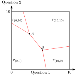
Figure 2: Four regions

For each corner $c$, define its opposite corner $n_{c}$, characterized as follows. For each $c\in C(X)$ there exists a unique $n_{c}\in C(X)$ such that for any $x\in X$, $x_{c}=s_{c}-x_{n_{c}}$, with $s_{c}$ the maximum answer that can be provided to the survey in the coordinate system $c$. Concretely, each answer to the survey admits an answer that is the exact opposite. In the case represented in Figure 2, corner $(0,0)$ has the opposite corner $(10,10)$. Let set $X^{*}=\{x^{*}\in X:u(x^{*})\geq u(x)\text{ for any }x\in X\}$, and set $Z^{*}$ characterized as follows:

$$Z^{*}=\{x\in X:\exists w\in C(X)\text{ and }u^{w}(x)=u^{n_{w}}(x)\leq u^{c}(x)\text{ for any }c\in C(X)\setminus\{w,n_{w}\}\}.$$ (7)

Observe that in Figure 2, $x\in X$ belongs to the segment $AB$ if:

$$u^{(0,0)}(x)=u^{(10,10)}(x)\leq\min(u^{(10,0)}(x),u^{(0,10)}(x)),$$ (8)

so $x\in Z^{*}$ for $w=(0,0)$ or $w=(10,10)$. I am now going to show that $X^{*}\subset Z^{*}$. To do that, I will show that $y\notin Z^{*}\implies y\notin X^{*}$, or equivalently, if for any $y\in X$, $y\notin Z^{*}$, then there exists a $x\in X$ such that $u(y)<u(x)$.

There are two cases to consider.

Case $1$: $y\in X$, and belongs to a region $r_{c}$ but $y$ is not on a boundary of $r_{c}$. That is, $u(y)=u^{c}(y)<\min_{w\in C(X)\setminus c}u^{w}(y)$. In that case, by continuity and monotonicity, there exists a small vector $\epsilon$ such that $\epsilon_{c}>0$ and $u(y+\epsilon)=u^{c}(y+\epsilon)>u^{c}(y)=u(y)$. This proves that $y$ cannot be a maximum of $u$.

Case $2$: $y\in X$, and belongs to the boundary between two adjacent regions and no opposite regions. That is:

$$u^{w}(y)=u^{z}(y)\leq\min_{c\in C(X)\setminus\{w,z\}}u^{c}(y)$$ (9)

with $z\notin n_{w}$, meaning $y$ belongs to the boundary of regions $r_{w}$ and $r_{z}$ but $w$ and $z$ are not opposite corners. If $w$ and $z$ are not opposite corners, then there necessarily exists a small perturbation $\epsilon$ such that $u^{w}(y+\epsilon)=u^{z}(y+\epsilon)$, and either $\epsilon_{w}>0$ or $\epsilon_{z}>0$. If $\epsilon_{w}>0$ without loss of generality, $u(y+\epsilon)=u^{w}(y+\epsilon)>u^{w}(y)=u^{w}(y)$, so $y$ does not maximize $u$.

To see why there necessarily exists a small perturbation $\epsilon$ such that $u^{w}(y+\epsilon)=u^{z}(y+\epsilon)$, and either $\epsilon_{w}>0$ or $\epsilon_{z}>0$, consider the case where $S=2$ depicted in Figure 2. Since corners $(0,0)$ and $(0,10)$ are adjacent, a downward slopping line from the perspective of the coordinate system with origin $(0,0)$ is an upward slopping line in the coordinate system with origin $(0,10)$. More generally, if $\epsilon_{w}=(\epsilon,\epsilon_{w,y})$, with $\epsilon>0$, then $\epsilon_{z}=(\epsilon,-\epsilon_{w,y})$, so either $\epsilon_{w}>0$ or $\epsilon_{z}>0$, depending on the sign of $\epsilon_{w,y}$. This intuition generalizes to any dimension $S>2$. This concludes the proof that $y\notin Z^{*}\implies y\notin x^{*}$, so $X^{*}\subset Z^{*}$

Restricting the feasible values of $x$ to $Z^{*}$, since $u^{w}(x)$ is linear in $x$, there is a unique $x^{*}\in X^{*}$ such that $x^{*}=\operatorname*{arg\,max}_{x\in Z^{*}}u^{w}(x)=u(x)$. By construction, $x^{*}=\operatorname*{arg\,max}_{x\in X}u(x)$. This shows the first property of single-peaked functions, according to Definition 5.

To prove the second property of single-peaked functions, take a segment that goes from $x^{*}$ to any $y\in X$ and that contains some $x\in X$. We can prove that $u(x^{*})\geq u(x)\geq u(y)$. Since $y,x,x^{*}$ belongs to the same straight line, there exists a coordinate system or corner $c$ such that $y_{c}\leq x_{c}\leq x^{*}_{c}$.

Remark 2

If there exists $c\in C(X)$ such that $y_{c}\leq x_{c}\leq x^{*}_{c}$, then $x$ and $y$ cannot be in opposite regions.

Proof. This remark can be demonstrated by contradiction. Assume that $x$ and $y$ belong to two opposite regions $w$ and $n_{w}$. Since $x\in r_{w}$, $x_{w}\leq x_{w}^{*}$. Since $y\in r_{n_{w}}$, $y_{n_{w}}\leq x_{n_{w}}^{*}$, so $y_{w}\geq x_{w}^{*}$. This implies that $x_{w}\leq x_{w}^{*}\leq y_{w}$. If $c=w$, then $x_{c}\leq x_{c}^{*}\leq y_{c}$, a contradiction. If $c=n_{w}$, following the same reasoning, we obtain the contradiction $y_{n_{w}}\leq x_{n_{w}}^{*}\leq x_{n_{w}}$. The last case to consider is $c\in C(X)\setminus\{w,n_{w}\}$. Since $c$ is different from $n_{w}$, $c\in C(X)$ is adjacent to $w$. Hence, $w$ and $c$ share the same coordinate in at least one dimension $s$. Concretely, the answer to question $s$ in coordinate $w$ is the same as the answer to question $s$ in the coordinate system $c$. Since $x_{s,c}=x_{s,w}\leq x_{s,c}^{*}=x_{s,w}^{*}\leq y_{s,c}=y_{s,w}$, $x_{c}\leq x^{*}\leq y_{c}$ cannot hold. $\blacksquare$

Using the previous remark, it is possible to reduce the number of cases to consider in the proof.

Case 1: $x,y,x^{*}\in r_{c}$. This is the simplest case, and it is direct that $u(x^{*})=u^{c}(x^{*})\geq u(x)=u^{c}(x)\geq u(y)=u^{c}(y)$ by monotonicity.

Case 2: $x,y\in r_{c}$ and $x^{*}\in r_{w}$ with $r_{c}$ and $r_{w}$ adjacent. In that case, there necessarily exists a point $z\in X$ on segment $yx^{*}$ such that $y_{c}\leq x_{c}\leq z_{c}\leq x^{*}_{c}$, and $z$ belongs to the boundary between regions $r_{c}$ and region $r_{w}$: $u^{c}(z)=u^{w}(z)$. In that case,

$$u(y)=u^{c}(y)\leq u(x)=u^{c}(x)\leq u(z)=u^{c}(z)$$

and

$$u^{w}(z)\leq u^{w}(x^{*})=u(x^{*}),$$

so

$$u(y)\leq u(x)\leq u(x^{*}).$$

Case 3: $y\in r_{c}$ and $x,x^{*}\in r_{w}$ with $r_{c}$ and $r_{w}$ adjacent. There necessarily exists a point $z\in X$ on segment $yx^{*}$ such that $y_{c}\leq z_{c}\leq x_{c}\leq x^{*}_{c}$, and $z$ belongs to the boundary between regions $r_{c}$ and region $r_{w}$: $u^{c}(z)=u^{w}(z)$. In that case,

$$u(y)=u^{c}(y)\leq u(x)=u^{c}(x)\leq u(z)=u^{c}(z)=u^{w}(z)$$

Moreover, the following inequalities are also verified:

$$u^{w}(z)=u(z)\leq u^{w}(x)=u(x)\leq u^{w}(x^{*})=u(x^{*}).$$

While $u^{w}(x)\leq u(x^{*})$ is immediate, the inequality $u^{w}(z)\leq u^{w}(x)$ stems from the shape of the indifference curves in the region $r_{w}$. If $z_{w}\geq x_{w}$, then since indifference curves are increasing in $r_{w}$, it is direct that $u^{w}(z)\leq u^{w}(x)$. If $z_{w}\geq x_{w}$ is not verified, then $u^{w}(z)\leq u^{w}(x)$ because the indifference curve going through $z$ in region $r_{w}$ is convex and downward slopping relative to origin $w$, so the maximum slope it takes in $z$ is the slope of segment $x^{*}z$. Indeed, otherwise, the indifference curve going through $z$ would go above $x^{*}$, contradicting that $x^{*}$ maximizes $u$. Since the slope of the segment $x^{*}z$ is equal to the slope of segment $xx^{*}$, $u^{w}(z)\leq u^{w}(x)$ is verified.

$\blacksquare$

4 Application

4.1 Data Description

I conducted a Priced Survey Methodology with 100 online participants recruited through Amazon Mechanical Turk. All participants had to answer a PSM consisting of the two following survey questions measuring altruism and self-interest:

On a scale from 0 to +10, where 0 indicates that you strongly disagree and +10 that you strongly agree, to what extent do you agree with these statements:

1. Individuals should primarily look after their own well-being before concerning themselves with the well-being of others.

2. Helping others, even when there’s no direct benefit to oneself, is a fundamental value that people should live by.

Participants filled out this survey for 9 consecutive rounds. They were paid $1 for completing the nine rounds and a short sociodemographic survey of seven questions. Table 1 provides summary statistics of individual characteristics.

Variables	Number of Participants
Female	23
Age
18-34	61
35+	39
Education
Low	17
Medium	14
High	69
Household income
under 34999	17
35000-49999	28
50000-74999	45
75000+	10
Occupation
Paid work	81
House work	11
Retired	2
Students	6
Marital status
married	88
single	12
Number of children
none	7
1	46
1+	47
Observations	100

• The low, medium, and high education levels correspond to primary, secondary, and university education, respectively. Household annual income is in $.

Table 1: Sociodemographic Variables.

Budget sets. In the first round, subjects can choose any answer to both questions on the $\{0,\dots,10\}$ scale. In the 8 following rounds, subjects are randomly presented with 8 different choice sets. The choice set of respondent $i$ in round $k\geq 1$, $B^{k}_{i}$, depends on $i$’s initial answer $q^{0}_{i}$:

$$B^{k}_{i}=\{q_{o^{k}}\in X\text{ such that }q_{o^{k}}.p^{k}\leq q^{0}_{i,o^{k}}.p^{k}-2\}.$$

That way, in any round $k\geq 1$, $q^{0}_{i}$ is not attainable but would have been with two more tokens. Since some respondents give answers close to one of the corners in round $0$, making $q^{0}_{i}$ not attainable in all rounds can turn out challenging. Hence, rounds such that $q_{o^{k}}.p^{k}\leq 2$ are excluded from the analysis. The price vectors are chosen so that budget sets intersect many times. As seen next, these aspects of the design imply that respondents can violate rationality. This is important, as if subjects behave rationality, it is not an artifact of the design but a feature of their decisions. Finally, the rounds are designed such that two out of eight rounds start from each of the four corners. Figure 3 gives the budget sets faced by two different respondents. In the left panel, the respondent initially provides a neutral answer to round $0$, $q^{0}=(5,5)$. Her budget sets in the following eight rounds are computed such that $q^{0}=(5,5)$ is never attainable, and two out of eight rounds start from each of the four corners. The black, blue, green, and red budget lines correspond to the rounds where the default answer is $(0,0)$, $(0,10)$, $(10,10)$, and $(10,0)$ respectively. In the right panel, the respondent initially provides a more asymmetrical answer, $q^{0}=(8,2)$, agreeing with question $1$ and disagreeing with question $2$.

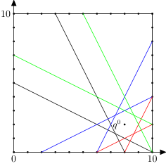
Figure 3: Examples of budget sets

4.2 Checking rationality

I begin by looking at respondents’ rationality when they fill out the PSM. For that, I introduce a slightly generalized version of the Critical Cost Efficiency Index (CCEI) introduced by Afriat (1972).

Definition 6

For subject $i\in\mathcal{I}$, and $e\in[0,1]$, an observed bundle $q^{k}\in X$ is

1. $e$-directly revealed preferred to a bundle $q$, denoted $q^{k}R^{0}_{e}q$, if $ep^{k}q^{k}_{o^{k}}\geq p^{k}q_{o^{k}}$ or $q_{o^{k}}=q^{k}_{o^{k}}$.

2. $e$-directly revealed strictly preferred to a bundle $q$, denoted $q^{k}P^{0}_{e}q$, if $ep^{k}q^{k}_{o^{k}}>p^{k}q_{o^{k}}$ or $q_{o^{k}}=q^{k}_{o^{k}}$.

3. $e$-revealed preferred to a bundle $q$, denoted $q^{k}R_{e}q$, if there exists a sequence of observed bundles $(q^{j},\dots,q^{m})$ such that $q^{k}R^{0}_{e}q^{j}$, …$q^{m}R^{0}_{e}q$.

4. $e$-revealed strictly preferred to a bundle $q$, denoted $q^{k}P_{e}q$, if there exists a sequence of observed bundles $(q^{j},\dots,q^{m})$ such that $q^{k}R^{0}_{e}q^{j}$, …$q^{m}R^{0}_{e}q$. and at least one of them is strict.

and

Definition 7

Let $e\in[0,1]$. A dataset $D=\{q^{k},B^{k}\}_{k\in\mathcal{K}}$ satisfies the general axiom of revealed preference at level $e$ (GARP_e) if for every pair of observed bundles, $q^{k}R_{e}q$ implies not $qP^{0}_{e}q^{k}$.

Afriat’s inconsistency index is

$$e^{*}=\max\{e\in[0,1]:\{q^{k},B^{k}\}_{k\in\mathcal{K}}\text{ satisfies }GARP_{e}\}.$$

Afriat’s inconsistency index is the most prevalent in the literature, and measures the extent of utility-maximizing behavior in the data. The main idea behind this index is that if expenditures at each observation are sufficiently “deflated”, then violations of GARP will disappear. The closer is the index to 1, the smaller it is necessary to shrink any budget to avoid GARP violation.

The violations of revealed preferences are summarized in Table 2. The average value of the CCEI index is 94%. As a comparison, Choi et al. (2014) finds an average CCEI of 88% in a standard consumption choice environment. Varian (1990) suggests a significance threshold of 95% for the CCEI index. Hence, even in uncontrolled and online experimental settings, subjects appear to behave rationally in the PSM. The average number of GARP violations in the sample is 1.7, with about 60% of the respondents with $0$ GARP violations.

	CCEI	GARP	Bronars	Time
Mean	0.94	1.69	0.45	277.20
Std	0.13	3.25	0.10	134.92
p5	0.61	0.00	0.34	87.90
p25	0.94	0.00	0.36	159.75
p50	1.00	0.00	0.43	258.50
p75	1.00	2.00	0.50	385.50
p95	1.00	9.30	0.64	480.50

• Column 1 gives the summary statistics of Afriat’s Critical Cost Efficiency Index (CCEI). Column 2 gives the summary statistics for the number of GARP violations. Column 3 gives the summary statistics for the Bronars’ index, and Column 4 gives the summary statistics for the time to complete the experiment in seconds.

Table 2: Summary Statistics: Rationality

The relatively high rationality of the respondents raises the question of how easy it is to violate rationality in this PSM design. Bronars (1987) designed a test that answers this question. The test measures the probability that a respondent with a random behavior would violate GARP in the consumption choice environment. Bronars’ test is widely applied in the literature on consumer choice and revealed preferences (Cox (1997), Mattei (2000), Andreoni and Miller (2002)). For example, Cox (1997) reports a Bronars power of 0.49 in a study of three consumption goods and seven budget rounds. With 11 budgets and two goods, Andreoni and Miller (2002) report a Bronars power of 78%. Since each individual faces different choice sets in the PSM, it is possible to perform Bronars’s test for each respondent. Column 3 of Table 2 reports the summary statistics of Bronars power test in the PSM. On average, the Bronars power is 45%, meaning that if answers to the PSM were made randomly, out of 1000 simulated choices, 45% would violate rationality. Hence, the Bronars’ power of this PSM design is relatively low. One reason why it is hard to achieve high indices in the PSM is that budget sets originate from different corners. Hence, they inherently intersect less than when they all originate from the same corner, as in the consumption choice environment. Future research might look at different designs that achieve higher Bronars scores. Increasing the Bronars’s scores might require adding more rounds, or setting individual-specific price vectors across rounds.

4.3 Estimating Preferences

Given that subjects’ answers are close to rational, it is worth recovering preferences behind survey answers. For subjects that do not consistently give corner answers, I will estimate the following single-peaked functional form:

$$u^{i}(q)=-\sum_{s=1}^{S}\frac{1}{2}a_{s}^{i}\left(q_{s}-b_{s}^{i}\right)^{2}.$$ (10)

Vector $\mathbf{b^{i}}=\{b^{i}_{s}\}_{s\in\mathcal{S}}$ measures respondent $i$’s ideal answer. It offers a robust alternative to the “ideal point” measured directly through the (cardinal) answer that respondents give to traditional surveys. The key difference with traditional surveys is that the ideal point $\mathbf{b^{i}}$ is measured using all rounds of the PSM. Vector $\mathbf{a^{i}}=\{a^{i}_{s}\}_{s\in\mathcal{S}}$ captures the relative significance that respondent $i$ places on different survey questions. Traditional surveys do not typically reveal the weight respondents assign to various questions, which can crucially influence their responses. For instance, a respondent might highly value altruism but might not prioritize expressing this in her answers relative to other survey topics. Without recognizing this distinction, one might mistakenly interpret such a response pattern as indicating lower altruism, rather than a differential emphasis on expressing altruistic values in the survey context.

With this specification, indifference curves are smooth and have an elliptic shape. Although more general specifications can be found, this one has the advantage of giving simple functional forms for the optimal answer to question $s$ in round $k$:

$$q_{1,o^{k}}=\alpha^{k}b_{1,o^{k}}+(1-\alpha^{k})\frac{R^{k}-p_{2}^{k}b_{2,o^{k}}}{p_{1}^{k}},$$ (11)

with $\alpha^{k}=\frac{a_{1}/(p_{1}^{k})^{2}}{a_{1}/(p_{1}^{k})^{2}+a_{2}/(p_{2}^{k})^{2}}$, and $q_{2,o^{k}}=(R^{k}-p_{1}^{k}q_{1,o^{k}})/p_{2}^{k}$, with $R^{k}=q^{0}_{i,o^{k}}.p^{k}-2$. It is as if a respondent was weighting providing an answer to question $1$ close to $b_{1}$ versus providing an answer to question $2$ close to $b_{2}$. If $\alpha^{k}$ is high, the respondent prefers to give an answer close to $b_{1}$ in observation $k$ and diverges from $b_{2}$ when she answers question $2$. Moreover, since $0<\alpha^{k}<1$, a respondent will never entirely “sacrifice” one question to give her ideal answer to the other question. She would rather try to answer both questions as close as she can to her ideal answer $(b_{1},b_{2})$. This property is akin to the taste for variety property of the CES specification commonly used in consumer theory.

Figure LABEL:fig_indif2 represents the indifference curves associated with the estimation of the utility function (10) for two respondents (respondent 65 and respondent 89). The indifference curves associated with the utility estimation for respondent 65 are represented in the left panel. Respondent 65 gives a corner answer to the traditional survey but her preferences are in fact less extreme. Using the PSM to estimate her ideal answer, we find $\mathbf{b}^{65}=(7.8,6.4)$. Moreover, this respondent appears to care more about question $2$ than question $1$, as $\mathbf{a}^{65}=(1.2,2.4)$, which seems at odd with the high answer provided to question $1$ to the traditional survey. The indifference curves associated with the utility estimation for respondent 94 are represented in the left panel. Respondent 94 cares relatively equally about the two questions, $\mathbf{a}^{94}=(1,0.75)$, but agrees relatively more with question 1 than with question 2, $\mathbf{b}^{94}=(4.3,2.1)$. For both respondents, there is a significant discrepancy between $\mathbf{b}^{i}$ and $q^{i,0}$.

Figure LABEL:fig:correl_b_q represents the correlations between $b_{s,i}$ and $q_{s}^{i,0}$ for the two questions. There is a weak positive correlation between $b_{i}$ and $q^{i,0}$. Taken at face value, this result would suggest that the answers provided to traditional surveys might not necessarily be good predictors of the ideal points that subjects have on scales. This intriguing result deserves further investigation in different PSM designs and larger datasets.

	$a_{1}$	$a_{2}$	$b_{1}$	$b_{2}$	$q_{1}^{0}$	$q_{2}^{0}$
Constant	1.653	$1.722^{*}$	$3.723^{**}$	$3.839^{***}$	$9.478^{***}$	$8.735^{***}$
	(1.010)	(1.014)	(1.504)	(1.384)	(1.258)	(1.326)
Age
18-34	$-0.801^{*}$	-0.345	0.799	0.819	-0.072	0.161
	(0.455)	(0.457)	(0.677)	(0.623)	(0.566)	(0.597)
Male	0.584	0.211	0.082	-0.656	0.088	0.211
	(0.497)	(0.499)	(0.740)	(0.681)	(0.619)	(0.653)
Education
Medium	$2.034^{***}$	$1.795^{**}$	$-2.553^{**}$	$-2.891^{***}$	$-1.563^{*}$	$-2.023^{**}$
	(0.731)	(0.734)	(1.088)	(1.001)	(0.910)	(0.960)
High	0.452	$1.027^{*}$	$-1.752^{**}$	$-1.597^{**}$	-0.746	-1.134
	(0.578)	(0.580)	(0.860)	(0.791)	(0.720)	(0.759)
Income
35000-49999	0.961	0.397	-0.772	-0.681	-1.234	-0.004
	(0.649)	(0.652)	(0.966)	(0.889)	(0.808)	(0.852)
50000-74999	0.349	-0.282	0.506	0.817	-0.787	0.145
	(0.614)	(0.616)	(0.914)	(0.841)	(0.765)	(0.806)
750000+	0.400	1.108	-2.119	-0.369	-0.030	0.570
	(0.876)	(0.880)	(1.305)	(1.200)	(1.091)	(1.151)
Number of Children
1	-0.452	0.022	0.396	0.769	0.089	-0.234
	(0.787)	(0.790)	(1.172)	(1.078)	(0.980)	(1.034)
1+	-0.283	-0.297	0.584	0.663	-0.101	0.194
	(0.790)	(0.793)	(1.176)	(1.082)	(0.984)	(1.038)
Observations	89	89	89	89	89	89
R2	0.224	0.151	0.177	0.190	0.104	0.081

• $\mathbf{a^{i}}$ and $\mathbf{b^{i}}$ are the parameters of the utility model (10) estimated using PSM data and a NLLS method. $q^{0}_{s}$ is the answer of subject $i$ to statement $s$ in round $0$, where $i$ faces no constraint on her choice set. 11 outliers were excluded from the data. For these respondents, the estimated utility parameters $\mathbf{a^{i}}$ and $\mathbf{b^{i}}$ were too extreme. The rule for exclusion of respondent $i$ is $a^{i}_{s}>15$, $a^{i}_{s}<0$, or $\mid b^{i}_{s}\mid>15$. This led to the exclusion of several respondents that violated rationality, leading to counterintuitive utility functions. Several of these outliers were rational but their Bronars’ scores were low, suggesting that rationality might be due to the experimental design for these respondents. ^∗ ($p<0.05$), ^∗∗ ($p<0.01$), ^∗∗∗($p<0.001$).

Table 3: Utility parameters explained by Sociodemographic Variables

Table 3 reports the summary statistics for the utility parameters, estimated using the non-linear least square method. Several patterns emerge. From column 1, parameter $a^{2}$ is significantly lower for the younger respondents. Hence, younger respondents seem to care less about expressing their self-interested preferences than older respondents. Similarly, the more educated respondents seem to care more about replying to the survey. Finally, from columns 3 to 6, respondents with medium to high education levels are significantly less altruistic and self-interested than the traditional survey predicts.

The PSM design used in this application can be improved in several ways. First, increasing the Bronars score could be achieved by increasing the number of rounds, or modifying the choice sets. Moreover, it might be pertinent to include more than one round where subjects can choose from the full choice set $X$. That way, it would be feasible to dynamically update the choice sets if respondents are not consistent when reporting their ideal answer. Finally, it might be worth testing the PSM with a payment that increases with the consistency of the answers provided to the PSM. That way, subjects might feel relatively more compelled to provide consistent answers than when their payment is unconditional.

5 Discussion

In this paper, I introduced a novel methodology to measure social preferences - the priced survey methodology. The PSM bridges the gap between decision theory and empirical survey data, enabling a more nuanced and precise exploration of how individuals form and express social preferences. The design of the PSM is close to experiments built to recover preferences from choices on linear budget sets as respondents fill the same survey multiple times under different choice sets.

The first key contribution of this paper is theoretical. I generalize Afriat’s theorem, and show that the Generalized Axiom of Revealed Preferences (GARP) is necessary and sufficient for the existence of a concave, continuous, and single-peaked utility function rationalizing survey answers. There are several important implications. First, rather than interpreting the cardinal answers subjects provide to a traditional survey, the PSM allows to estimate utility parameters. These utility parameters offer a robust ground for comparing social preferences. Moreover, by estimating the peak of the utility function rationalizing PSM answers, experimenters have access to a novel measure of a respondent’s ideal answer to a survey. Finally, the PSM allows experimenters to measure aspects of social preferences that cannot be captured with traditional surveys such as the relative importance that respondents give to different survey questions.

A simple PSM design is implemented in a sample of 100 online participants. All participants had to answer a PSM consisting of nine rounds and two questions measuring altruistic and self-interested preferences. Several interesting patterns emerge. First, I find that respondents reach an average CCEI score of 94%. Moreover, I used the individual-level data to estimate a smooth, concave, and single-peaked utility function. Although the low number of participants makes it difficult to interpret the results, it seems that older and more educated respondents care relatively more about answering the survey. The more educated respondents are also significantly less altruistic and self-interested than the traditional survey predicts. Finally, I find a weak positive correlation between respondents’ ideal points, as estimated through the PSM, and respondents’ answers to the traditional survey.

Future studies have the potential to refine the PSM’s design, increasing in particular the Bronars scores. Such advancements are pivotal for an in-depth analysis of the rational underpinnings of social preferences. In this context, Seror (2023)’s methodology for estimating behavioral biases through choice rankings might present a promising avenue. Additionally, extending the application of the PSM to various domains, including behavioral economics, social psychology, and public policy—could offer deeper insights into the complex layers of social preference dynamics. These explorations are not only crucial for theoretical advancements but also bear significant implications for practical interventions and policy formulations.

Appendix

Appendix A Proof of Theorem 1

The proof that $4\Rightarrow 1$ is direct, and $3\Rightarrow 4$ has been proven in the main text. It remains to be proven that $2\Rightarrow 3$, and $1\Leftrightarrow 2$.

Proof that $2\Rightarrow 3$. The following is a constructive proof that follows the standard proof of Afriat’s Theorem, as detailed by Chambers and Echenique (2016, p.45).

Consider the revealed preference pair $(\succcurlyeq^{R},\succ^{R})$ restricted to $X^{0}$. GARP implies that there is a preference relation $\succcurlyeq$ on $X^{0}$ such that $x\succcurlyeq y$ when $x\succcurlyeq^{R}y$, and $x\succ y$ when $x\succ^{R}y$. Partition $X^{0}$ according to the equivalence classes of $\succcurlyeq$. That is, let $I_{1},\dots,Y_{J}$ be a partition of $X^{0}$ such that $x\sim y$ for $x,y\in I_{j}$ and $x\succ y$ if $x\in I_{j}$, $y\in I_{h}$ and $j>h$.

Define $(U^{k},\lambda^{k})_{k\in\mathcal{K}}$ recursively. Let $U^{k}=\lambda^{k}=1$ if $x^{k}\in I_{J}$.

Suppose that we have defined $(U^{k},\lambda^{k})$ for all $x^{k}\in\bigcup_{h=j+1}^{J}I_{h}$. We can choose $V_{j}$ such that, for all $x^{l}\in I_{j}$ and $x^{k}\in\bigcup_{h=j+1}^{J}I_{h}$,

$$V_{j}<U^{k}$$

and

$$V_{j}<U^{k}+\lambda^{k}p^{k}.(x^{l}_{o^{k}}-x^{k}_{o^{k}}).$$ (A.1)

Set $U^{l}=V_{j}$ for all $l$ with $x^{l}\in I_{j}$.

Given this choice of $U^{l}$, if $x^{k}\in\bigcup_{h=j+1}^{J}I_{h}$, then $U^{l}<U^{k}$. Moreover, since $p^{l}.(x^{k}_{o^{l}}-x^{l}_{o^{l}})>0$, it is possible to characterize $\lambda^{l}$ as:

$$\lambda^{l}=\max_{k}\frac{U^{k}-U^{l}}{p^{l}.(x^{k}_{o^{l}}-x^{l}_{o^{l}})}\geq 0$$ (A.2)

where the max is taken over the values of $k$ such that $x^{k}\in\bigcup_{h=j+1}^{J}I_{h}$.

The chosen $(U^{k},\lambda^{k})_{k\in\mathcal{K}}$ satisfy the system of inequalities (2). Indeed, let $k$ and $l$ be such that $x^{k}\in I_{j}$, and $x^{l}\in I_{h}$ with $j>h$. Then (A.1) ensures that

$$U^{l}\leq U^{k}+\lambda^{k}p^{k}.(x^{l}_{o^{k}}-x^{k}_{o^{k}}).$$

and equation (A.2) ensures that

$$U^{k}\leq U^{l}+\lambda^{k}p^{l}.(x^{k}_{o^{l}}-x^{l}_{o^{l}}).$$

If $k$ and $l$ are such that $x^{k},x^{l}\in I_{j}$, then $U^{k}=U^{l}$, so $U^{k}\leq U^{l}+\lambda^{k}p^{l}.(x^{k}_{o^{l}}-x^{l}_{o^{l}})$ because $p^{l}.(x^{k}_{o^{l}}-x^{l}_{o^{l}})\geq 0$, and $U^{l}\leq U^{k}+\lambda^{k}p^{k}.(x^{l}_{o^{k}}-x^{k}_{o^{k}})$ because $p^{k}.(x^{l}_{o^{k}}-x^{k}_{o^{k}})\geq 0$

Proof that $1\Leftrightarrow 2$. The proof below closely follows the steps of the proof of Theorem 3.1 in Chambers and Echenique (2016, p. 37).

Theorem 2

In any observation $k$, $(\geq,>)$ is an acyclic order pair, and for any $(x,y)\in B^{k}$, it satisfies $x_{o^{k}}>y_{o^{k}}\geq z$ $\Rightarrow$ $x_{o^{k}}>z_{o^{k}}$. There exists a preference relation which is c-monotonic with respect to the order pair $(\geq,>)$ and which weakly rationalizes the data iff $(\succcurlyeq^{R},\succ^{R})$ satisfies GARP.

Assume that $\succcurlyeq$ is c-monotonic and weakly rationalizes the data $D$. Assume moreover that $(\succcurlyeq^{R},\succ^{R})$ does not satisfy GARP. Hence, there exists a sequence of observations in $D$ $x^{1},\dots,x^{L}$ such that

$$x^{1}\succcurlyeq^{R}\dots\succcurlyeq^{R}x^{L}\text{ and }x^{L}\succ^{R}x^{1}$$

As $x^{L}\succ^{R}x^{1}$ and $B^{L}$ is comprehensive in the coordinate system with origin $o^{L}$, there exists $z\in B^{L}$ such that $x^{L}\succcurlyeq^{R}z$ and $z_{o^{L}}>x^{1}_{o^{L}}$.

Since $\succcurlyeq$ weakly rationalizes D, $x^{1}\succcurlyeq\dots\succcurlyeq x^{L}\succcurlyeq z$. By c-monotonicity, since $z_{o^{L}}>x^{1}_{o^{L}}$, $z\succ x^{1}$, a contradiction that $\succcurlyeq$ is a preference relation.

Conversely, assume that $(\succcurlyeq^{R},\succ^{R})$ is an acyclic order pair. Let’s show that $(\succcurlyeq^{R}\cup\geq,>)$ is also an acyclic order pair. To do that, we make first three key observations. For any observation $k$, and pair $(x,y)\in B^{k}$

1. $x\succcurlyeq^{R}y$ and $y_{o^{k}}\geq z_{o^{k}}$ $\Rightarrow$ $x\succcurlyeq^{R}z$.

2. $x\succcurlyeq^{R}y$ and $y_{o^{k}}>z_{o^{k}}$ $\Rightarrow$ $x\succ^{R}z$.

3. $x\succ^{R}y$ and $y_{o^{k}}\geq z_{o^{k}}$ $\Rightarrow$ $x\succ^{R}y$.

Assume that $(\succcurlyeq^{R}\cup\geq,>)$ is not acyclic and let $Q=\succcurlyeq^{R}\cup\geq$. There exists a sequence of observations in $D$ such that $x^{1}Q\dots Qx^{L}$ and $x^{L}_{o^{L}}>x^{1}_{o^{1}}$. Without loss of generality, the cycle can be rewritten as

$$x^{1}_{o^{1}}\geq x^{2}_{o^{1}},x^{2}_{o^{2}}\geq x^{3}_{o^{2}},x^{3}_{o^{3}}\geq x^{4}_{o^{3}},\dots x^{p-1}_{o^{p-1}}\geq x^{p}_{o^{p-1}}\text{, }x^{p}\succcurlyeq^{R}\dots\succcurlyeq^{R}x^{L}\text{, and }x^{L}_{o^{L}}>x^{1}_{o^{L}}.$$

If $p\neq L$, $x^{L-1}\succcurlyeq^{R}x^{L}$ and $x^{L}{o^{L}}>x^{1}_{o^{L}}$ implies, from observation 2, that $x^{L-1}\succ^{R}x^{1}$. Repeating the same reasoning using the inequality $x^{1}_{o^{1}}\geq x^{2}_{o^{1}}$, we obtain $x^{L-1}\succ^{R}x^{2}$. Repeating again in an iterative way, we obtain $x^{L-1}\succ^{R}x^{p}$. Hence, $x^{p}\succcurlyeq^{R}\dots\succcurlyeq^{R}x^{L-1}\succ^{R}x^{p}$, contradicting that $(\succcurlyeq^{R},\succ^{R})$ is acyclic. This implies that $(\succcurlyeq^{R}\cup\geq,>)$ is an acyclic order pair.

As $(\succcurlyeq^{R}\cup\geq,>)$ is an acyclic order pair, there is a preference relation $\succcurlyeq$ such that $\succcurlyeq^{R}\subseteq\succcurlyeq$, $\geq\subseteq\succcurlyeq$, and $>\subseteq\succ$ (Theorem 1.5 in Chambers and Echenique (2016, p. 7)). As a consequence, $\succcurlyeq$ is c-monotonic with respect to $(\geq,>)$ and weakly rationalizes $D$.

References

- (1)
- Abeler, Nosenzo and Raymond (2019) Abeler, Johannes, Daniele Nosenzo and Collin Raymond. 2019. “Preferences for Truth-Telling.” Econometrica 87(4):1115–1153.
- Afriat (1967) Afriat, S. N. 1967. “The Construction of Utility Functions from Expenditure Data.” International Economic Review 8(1):67–77.
- Afriat (1972) Afriat, Sidney N. 1972. “Efficiency Estimation of Production Function.” International Economic Review 13(3):568–98.
- Andreoni and Miller (2002) Andreoni, James and John Miller. 2002. “Giving According to GARP: An Experimental Test of the Consistency of Preferences for Altruism.” Econometrica 70(2):737–753.
- Bond and Lang (2019) Bond, Timothy N. and Kevin Lang. 2019. “The Sad Truth about Happiness Scales.” Journal of Political Economy 127(4):1629–1640.
- Bossert and Peters (2009) Bossert, Walter and Hans Peters. 2009. “Single-Peaked Choice.” Economic Theory 41(2):213–230.
- Bronars (1987) Bronars, Stephen G. 1987. “The Power of Nonparametric Tests of Preference Maximization.” Econometrica 55(3):693–698.
- Chambers and Echenique (2016) Chambers, Christopher P. and Federico Echenique. 2016. Revealed Preference Theory. Econometric Society Monographs Cambridge University Press.
- Choi et al. (2007) Choi, Syngjoo, Raymond Fisman, Douglas Gale and Shachar Kariv. 2007. “Consistency and Heterogeneity of Individual Behavior under Uncertainty.” American Economic Review 97(5):1921–1938.
- Choi et al. (2014) Choi, Syngjoo, Shachar Kariv, Wieland Müller and Dan Silverman. 2014. “Who Is (More) Rational?” American Economic Review 104(6):1518–50.
- Cox (1997) Cox, James C. 1997. “On Testing the Utility Hypothesis.” Economic Journal 107(443):1054–1078.
- Desmet, Ortuño-Ortín and Wacziarg (2017) Desmet, Klaus, Ignacio Ortuño-Ortín and Romain Wacziarg. 2017. “Culture, Ethnicity, and Diversity.” American Economic Review 107(9):2479–2513.
- Echenique, Lee and Shum (2011) Echenique, Federico, Sangmok Lee and Matthew Shum. 2011. “The Money Pump as a Measure of Revealed Preference Violations.” Journal of Political Economy 119(6):1201–1223.
- Falk et al. (2018) Falk, Armin, Anke Becker, Thomas Dohmen, Benjamin Enke, David Huffman and Uwe Sunde. 2018. “Global Evidence on Economic Preferences*.” The Quarterly Journal of Economics 133(4):1645–1692.
- Fehr and Schmidt (1999) Fehr, Ernst and Klaus M. Schmidt. 1999. “A Theory of Fairness, Competition, and Cooperation.” The Quarterly Journal of Economics 114(3):817–868.
- Fisman et al. (2015) Fisman, Raymond, Pamela Jakiela, Shachar Kariv and Daniel Markovits. 2015. “The distributional preferences of an elite.” Science 349(6254):aab0096.
- Forges and Minelli (2009) Forges, Françoise and Enrico Minelli. 2009. “Afriat’s theorem for general budget sets.” Journal of Economic Theory 144(1):135–145.
- Halevy, Persitz and Zrill (2018) Halevy, Yoram, Dotan Persitz and Lanny Zrill. 2018. “Parametric Recoverability of Preferences.” Journal of Political Economy 126(4):1558–1593.
- Henrich et al. (2001) Henrich, Joseph, Robert Boyd, Samuel Bowles, Colin Camerer, Ernst Fehr, Herbert Gintis and Richard McElreath. 2001. “In Search of Homo Economicus: Behavioral Experiments in 15 Small-Scale Societies.” American Economic Review 91(2):73–78.
- Houtman and Maks (1985) Houtman, M and J Maks. 1985. “Determining all Maximal Data Subsets Consistent with Revealed Preference.” Kwantitatieve Methoden 19:89–104.
- Mattei (2000) Mattei, Aurelio. 2000. “Full-scale real tests of consumer behavior using experimental data.” Journal of Economic Behavior & Organization 43(4):487–497.
- Nishimura, Ok and Quah (2017) Nishimura, Hiroki, Efe A. Ok and John K.-H. Quah. 2017. “A Comprehensive Approach to Revealed Preference Theory.” American Economic Review 107(4):1239–63.
- Polisson, Quah and Renou (2020) Polisson, Matthew, John K.-H. Quah and Ludovic Renou. 2020. “Revealed Preferences over Risk and Uncertainty.” American Economic Review 110(6):1782–1820.
- Polisson and Renou (2016) Polisson, Matthew and Ludovic Renou. 2016. “Afriat’s Theorem and Samuelson’s ‘Eternal Darkness’.” Journal of Mathematical Economics 65(C):36–40.
- Seror (2023) Seror, Avner. 2023. “A Semi-Parametric Approach to Behavioral Biases.” Working Paper .
- Stantcheva (2023) Stantcheva, Stefanie. 2023. “How to Run Surveys: A Guide to Creating Your Own Identifying Variation and Revealing the Invisible.” Annual Review of Economics 15(1):205–234.
- Varian (1990) Varian, Hal. 1990. “Goodness-of-fit in optimizing models.” Journal of Econometrics 46(1-2):125–140.
- Varian (1982) Varian, Hal R. 1982. “The Nonparametric Approach to Demand Analysis.” Econometrica 50(4):945–973.