Joint 3D User and 6D Hybrid Reconfigurable Intelligent Surface Localization

Abstract

The latest assessments of the emerging technologies for ris have indicated the concept’s significant potential for localization and sensing, either as individual or simultaneously realized tasks. However, in the vast majority of those studies, the RIS state (i.e., its position and rotation angles) is required to be known a priori. In this paper, we address the problem of the joint three-dimensional (3D) localization of a hybrid RIS (HRIS) and a user. The most cost- and power-efficient hybrid version of an RIS is equipped with a single reception radio-frequency chain and meta-atoms capable of simultaneous reconfigurable reflection and sensing. This dual functionality is controlled by adjustable power splitters embedded at each hybrid meta-atom. Focusing on a downlink scenario where a multi-antenna base station transmits multi-carrier signals to a user via an HRIS, we propose a multi-stage approach to jointly estimate the metasurface’s 3D position and 3D rotation matrix (i.e., 6D parameter estimation) as well as the user’s 3D position. Our simulation results verify the validity of the proposed estimator via extensive comparisons of the root-mean-square error of the state estimations with the crb, which is analytically derived. Furthermore, it is showcased that there exists an optimal hris power splitting ratio for the desired multi-parameter estimation problem. We also study the robustness of the proposed method in the presence of scattering points in the wireless propagation environment.

I Introduction

REconfigurable intelligent surfaces (ris) are recently being extensively studied as an enabling technology for the upcoming 6g of wireless systems [1, 2]. An ris is a planar surface made of sub-wavelength unit cells with controllable em properties [3, 4]. In essence, ris can modify wave characteristics such as phase, amplitude, frequency, and even polarization, offering radio propagation control [5, 6, 7]. Smart wireless environments can be achieved via this characteristic of ris, which provides coverage extension and localization, as well as sensing capabilities [8, 9]. Hence, ris are expected to be the vital enabler for the 6g of wireless systems [10, 11], where joint communications and localization is expected to aid various use cases [12], such as connected robotics, autonomous systems, and other immersive applications [13]. There have been several studies on ris’s utility in radio localization by developing localization algorithms or deriving crb, see, e.g., [14, 15, 16, 17, 18, 19, 20, 21, 22, 23, 24, 25, 26, 27, 28, 29]. In those works, ris have been successfully deployed for ue radio localization in two different general scenarios. In the first scenario, except for the bs, the ris acts as anchor with known state, i.e., location and orientation. These kind of systems are known as RIS-aided or RIS-enabled localization [30], and exploit reflected signals from ris to improve or assist ue localization. In the second scenario, a ue can use an RIS(s) to enable its localization, where the RIS(s)’s state is unknown and needs to be estimated. This problem is known as RIS localization, which one can see as a bi-static sensing or a calibration problem [26].

RIS-aided ue localization has been intensely studied in recent years, ranging from two-dimensional (2D) to 3D scenarios under either ff or nn operating conditions, as well as indoor and outdoor scenarios [31, 32, 14, 15, 16, 17, 18, 19, 20, 21, 22, 23, 24, 25, 33, 34, 35, 36, 37]. ue localization under the nn condition via analyzing the crb has been studied in [14] for passive ris, and for hybrid ris (hris) with los blockage in [18]. Moreover, the possibility of ue positioning under nlos harsh propagation conditions has been shown [32, 24], in which the ris is equipped with a large number of reflecting elements. In [20], the authors showed that the fim on the ue position estimation, in the case it operates in the  nn regime, quadratically increases with the size of the ris. Furthermore, a ue localization algorithm based on compressed sensing techniques for an uplink nn scenario was presented in [21]. 3D ue localization and synchronization in the ff scenario has been studied in [15, 16], where ue mobility and the spatial-wideband effect were taken into account. In [19, 29], multiple ris were adopted for ue localization. In [19], the ris modulate an impinging unmodulated carrier and time-difference-of-arrival is calculated at the receivers to estimate the UE location. The localization approach in [29] considered narroband transmission and was based in aoa estimation. In [25], the potential of using an ris for ue orientation estimation, besides its location estimation, was studied via an crb analysis.

The problem of RIS localization, which assumes that the ris state (i.e., position and/or orientation) is unknown, has been rarely discussed. While lack of knowledge of the RIS position and orientation generally does not affect RIS-aided communication, it prevents RIS-aided UE localization [38]. The RIS position or orientation may be unknown for a number of reasons, including poor calibration, lack of knowledge of the environment map in which the RIS is placed, or due to mobility of the RIS itself [39, 40]. The relevant works are only [26, 28] that focused on a passive ris. In these works, the locations of the transmitters and receivers are assumed to be known, which requires some overhead for infrastructure calibration. The estimation of aoa and aod separately at the ris offers a promising way for ris localization jointly with the localization of one of the transmitter and receiver [27], reducing the aforementioned calibration overhead. However, one cannot separately estimate the aoa and aod at the passive ris. Adding sensing capability to the ris can be a promising solution to overcome this challenge [27], which was first proposed in [41] for individual channel estimation. This version of an ris was then extended in [42, 43, 44] to a HRIS that is capable of simultaneous reflection and sensing. According to this RIS hardware architecture, waveguides feed the incident signals at each hybrid meta-atom to reception (RX) rf chains, which is connected to a baseband unit. This reception mechanism effectively acts as an analog combiner whose phase shifts can be dynamically optimized [42]. Very recently, [18] studied UE localization in an NF scenario, considering multiple RX rf chains at the HRIS and that its state is precisely known. HRIS-assisted MIMO radar-communication systems has been investigated, where the HRIS simultaneously reflected communications signals and received radar echos [45]. However, HRISs with a single RX rf chain in localization problems, where their states are unknown, have not yer been investigated.

In this paper, we extend our recent work in [27], which addressed joint 2D ue and hris localization, to joint 3D ue and hris localization under ff conditions, including the 3D rotation matrix estimation for the HRIS. The main contributions of this paper are summarized as follows.

• We devise a multi-stage algorithm for joint multiple-input-single-output (MISO) 3D localization and synchronization of a ue and an hris under ff scenarios. In the first step, we estimate the geometric parameters of the associated channels, i.e., delay, gain, aoa/aod at hris, and aod at the BS. The aoa/aod estimation at the HRIS is enabled by its single RX RF chain. Using these estimations at a further stage, we calculate the 3D position and clock bias of the ue and the hris. At the final step of the proposed approach, we make use of the positions’ estimates, the aoa at the HRIS from the BS and the aod from the HRIS to the ue to estimate the 3D rotation matrix of the HRIS.

• We investigate the role of several system parameters (the transmit power at the BS, the power splitting ratio at the hris, and the presence of scatterers) on the error of the proposed estimation approach via extensive simulations, and through comparisons with the estimator’s crb, which is derived for this purpose. In this investigation, we consider hris phase profiles from the dft. Our simulation results showcase the efficiency of the proposed estimatin algorithm, which attains the corresponding crb at high transmit power levers. The critical role of the hris power splitting ratio on the localization performance is also unveiled. We finally show that the proposed approach is robust to the presence of the scattering points (SPs).

The rest of this paper is organized as follows: In Section II, the system and signal models are described, while the Fisher information of the estimations is detailed in Section III. The proposed estimation algorithm is presented in Section IV. In Section V, we numerically evaluate the rmse of the parameters’ estimation and compare it with the respective crb. Section VI concludes the paper.

Notation

Vectors and matrices are indicated by lowercase and uppercase bold letters, respectively. The element in the $i$-th row and $j$-th column of matrix $\mathbf{A}$ is denoted by $\left[\mathbf{A}\right]_{i,j}$ and $\det(\mathbf{A})$ returns $\mathbf{A}$’s determinant. The sub-index $i:j$ determines all the elements between $i$ and $j$. The complex conjugate, Hermitian, transpose, and Moore–Penrose inverse operators are represented by $\left(.\right)^{*}$, $\left(.\right)^{\mathsf{H}}$, $\left(.\right)^{\top}$, and $\left(.\right)^{\dagger}$, respectively. $\|.\|$ calculates the norm of vectors or Frobenius norm of matrices. $\odot$ and $\otimes$ indicate the element-wise and Kronecker products, respectively. $\mathbb{R}$ and $\mathbb{C}$ are the real and complex number sets, $\Re\{\cdot\}$ and $\Im\{\cdot\}$ give the real and imaginary parts of a complex number, and $\jmath=\sqrt{-1}$. $\mathbf{1}_{K}$ and $\mathbf{0}_{K}$ are column vectors with length $K$ comprising all ones and zeros, respectively. The functions $\text{atan2}(y,x)$ and acos(x) are the four-quadrant inverse tangent and inverse cosine functions, respectively.

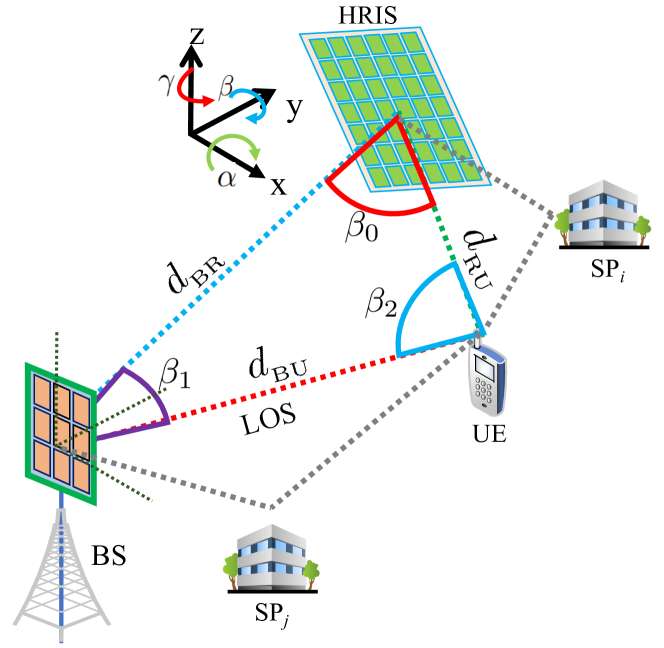
Figure 1: The considered wireless system comprising a multi-antenna BS, a single-antenna UE, and a single-RX-RF HRIS. The 3D location of the UE and the 6D state of the HRIS are unknown.

II System and Signal Models

In this section, we introduce the considered HRIS-empowered system model as well as the models for the received signals and the wireless channel that will be deployed for the proposed localization approach.

II-A System Setup

Consider the wireless system scenario in Fig. 1 consisting of one $M_{{}_{\text{B}}}$-antenna BS with a known location $\mathbf{p}_{\text{B}}\in\mathbb{R}^{3}$, one single-antenna UE with an unknown location $\mathbf{p}_{\text{U}}\in\mathbb{R}^{3}$, and an HRIS with unknown location $\mathbf{p}_{\text{R}}\in\mathbb{R}^{3}$ and unknown orientation. We consider the downlink scenario where the BS sends $T$ orthogonal frequency division multiplexing (OFDM) symbols over time via $K$ subcarriers. We assume that all the associated channels remain constant during each transmission time slot. To model the HRIS orientation, we use a rotation matrix $3\times 3$ matrix $\mathbf{R}$ that determines local coordinate frames, which belongs in the special orthogonal group SO(3), i.e., orthogonal matrices with unit-valued determinant. In particular, we define a reference orientation where the axes are in the same direction as those of the global coordinate frame, as shown in Fig. 1. We assume that the global coordinate system is aligned with the BS local coordinate system. Accordingly, we can express the HRIS rotation matrix as follows:

$$\mathbf{R}=\mathbf{R}_{\alpha}(z)\mathbf{R}_{\beta}(y)\mathbf{R}_{\gamma}(x),$$ (1)

where $\mathbf{R}_{\beta}(z)$, $\mathbf{R}_{\beta}(y)$, and $\mathbf{R}_{\beta}(x)$ represent the rotation matrices w.r.t. $z$-axis, $y$-axis, and $x$-axis, respectively, and are expressed as follows:

$$\mathbf{R}_{\alpha}(z)=\begin{bmatrix}\cos{\alpha}&\sin{\alpha}&0\\ -\sin{\alpha}&\cos{\alpha}&0\\ 0&0&1\end{bmatrix},$$ (2a)

$$\mathbf{R}_{\beta}(y)=\begin{bmatrix}\cos{\beta}&0&\sin{\beta}\\ 0&1&0\\ -\sin{\beta}&0&\cos{\beta}\end{bmatrix},$$ (2b)

$$\mathbf{R}_{\gamma}(x)=\begin{bmatrix}1&0&0\\ 0&\cos{\gamma}&-\sin{\gamma}\\ 0&\sin{\gamma}&\cos{\gamma}\end{bmatrix}.$$ (2c)

The direction vectors from the HRIS to the BS and the UE in the local coordinate system can be respectively obtained as:

$$\mathbf{q}_{\text{RB}}=\mathbf{R}^{\top}(\mathbf{p}_{\text{B}}-\mathbf{p}_{\text{R}})/\|\mathbf{p}_{\text{B}}-\mathbf{p}_{\text{R}}\|,$$ (3a)

$$\mathbf{q}_{\text{RU}}=\mathbf{R}^{\top}(\mathbf{p}_{\text{U}}-\mathbf{p}_{\text{R}})/\|\mathbf{p}_{\text{U}}-\mathbf{p}_{\text{R}}\|.$$ (3b)

Similarly, we respectively write the direction vectors from the BS to the HRIS and the UE in the BS coordinate system as:

$$\mathbf{q}_{\text{BR}}=(\mathbf{p}_{\text{R}}-\mathbf{p}_{\text{B}})/\|\mathbf{p}_{\text{R}}-\mathbf{p}_{\text{B}}\|,$$ (4a)

$$\mathbf{q}_{\text{BU}}=(\mathbf{p}_{\text{U}}-\mathbf{p}_{\text{B}})/\|\mathbf{p}_{\text{U}}-\mathbf{p}_{\text{B}}\|.$$ (4b)

Moreover, the HRIS and UE are assumed unsynchronized with the BS, leading to the unknown clock biases $b_{\text{R}}$ and $b_{\text{U}}$ at the HRIS and UE, respectively, with respect to the BS. Therefore, in addition to the HRIS location and UE position, the latter clock bias components need to be estimated.

The BS is assumed equipped with a uniform planar array (UPA) with $M_{{}_{\text{B}}}=M_{{}_{\text{B}}}^{r}\times M_{{}_{\text{B}}}^{c}$ elements. The element in each $r$th row ($r\in\{0,\dots,M_{{}_{\text{B}}}^{r}-1\}$) and $s$th column ($s\in\{0,\dots,M_{{}_{\text{B}}}^{c}-1\}$) has the position $\mathbf{q}_{r,s}=[d(2r-M_{{}_{\text{B}}}^{r}+1)/2),0,d(2s-M_{{}_{\text{B}}}^{c}+1)/2)]^{\top}$ in the local coordinate system of the BS, with $d$ being the spacing between the elements. Similarly, the HRIS is a UPA with $M_{{}_{\text{R}}}=M_{{}_{\text{R}}}^{r}\times M_{{}_{\text{R}}}^{c}$ unit elements, all attached via a dedicated waveguide to a single RX RF chain [42], enabling simultaneous tunable reflection and sensing of impinging signals. Accordingly, each $(n,m)$th element ($n\in\{0,\dots,M_{{}_{\text{R}}}^{r}-1\}$ and $m\in\{0,\dots,M_{{}_{\text{R}}}^{c}-1\}$) of the HRIS has the position $\mathbf{q}_{n,m}=[d(2n-M_{{}_{\text{R}}}^{r}+1)/2),0,d(2m-M_{{}_{\text{R}}}^{c}+1)/2)]^{\top}$ in the local coordinate system of the HRIS. We assume for both the BS and HRIS that $d\leq\lambda/2$ with $\lambda$ being the carrier frequency wavelength. We further assume that the UE operates in the FF range of the BS and the HRIS. Our final assumption is that the HRIS and the UE share their observations with a fusion center (FC) via a reliable link [46]. The FC is responsible for carrying out, the targeted in this paper, joint location estimation of the UE and the HRIS, which we will be presented in the sequel.

II-B Signal and Channel Models

The HRIS is capable of simultaneously sensing and reflecting its impinging signals. To this end, it possesses $M_{{}_{\text{R}}}$ identical power splitters within its structure to divide the received signal power at each meta-atom into two parts [42, 43, 44]: one for reflection and the other for sensing/reception. For the latter operation, the HRIS adopts a phase shifting network to feed a portion of the impinging signals on its elements to the single RX RF chain. Mathematically, this phase shifting network applies a combining vector modeled by $\mathbf{c}_{{}_{t}}\in\mathbb{C}^{M_{{}_{\text{R}}}}$ with $|[\mathbf{c}_{{}_{t}}]_{i}|=1$ $\forall$ $i=1,\ldots,M_{{}_{\text{R}}}$ during each time interval $t$. Each $i$-th HRIS unit element also reflects the remaining portion of its impinging signal at each time $t$, which is modeled by the phase shift $[\boldsymbol{\gamma}_{{}_{t}}]_{i}$ with $\boldsymbol{\gamma}_{t}\in\mathbb{C}^{M_{{}_{\text{R}}}}$ and $|[\boldsymbol{\gamma}_{{}_{t}}]_{i}|=1$. We make the assumation that the FC has complete knowledge about the HRIS combining vector and phase profile. We further assume that the multi-antenna BS applies the dft codebook for its beamforming vector $\mathbf{f}_{{}_{t}}\in\mathbb{C}^{M_{{}_{\text{B}}}}$ at each time instant $t$, and transmits unit-power symbols.

Under the above assumptions, after cyclic prefix removal and fast Fourier transform (FFT) application, the received signals at the HRIS and the UE at each time instant $t$, which are respectively denoted by the matrices $\mathbf{y}_{{}_{\text{R}},_{t}}\in\mathbb{C}^{K}$ and $\mathbf{y}_{{}_{\text{U}},_{t}}\in\mathbb{C}^{K}$, can be expressed as follows:

$$\mathbf{y}_{{}_{\text{R},t}} =g_{{}_{\text{BR}}}\sqrt{\rho P_{\text{B}}}\mathbf{d}(\tau_{{}_{\text{BR}}})\,\mathbf{c}_{{}_{t}}^{\top}\mathbf{a}_{{}_{\text{R}}}(\boldsymbol{\phi}_{{}_{\text{RB}}})\mathbf{a}^{\top}_{{}_{\text{B}}}(\boldsymbol{\theta}_{{}_{\text{BR}}})\mathbf{f}_{{}_{t}}+\mathbf{w}_{{}_{\text{R}},_{t}},$$ (5a)

$$\mathbf{y}_{{}_{\text{U},t}} =\mathbf{y}_{{}_{\text{BU}},_{t}}+\mathbf{y}_{{}_{\text{BRU}},_{t}}+\mathbf{y}^{s}_{{}_{\text{BU}},_{t}}+\mathbf{y}^{s}_{{}_{\text{BRU}},_{t}}+\mathbf{w}_{{}_{\text{U}},_{t}},$$ (5b)

where $g_{{}_{\text{BR}}}$ denotes the unknown complex gain of the BS-HRIS link, $P_{\text{B}}$ is the BS transmit power, $\rho$ represents the common power splitting ratio at each hybrid meta-atom used for the sensing operation, and $\mathbf{w}_{{}_{\text{R}},_{t}}\in\mathbb{C}^{K}$ and $\mathbf{w}_{{}_{\text{U}},_{t}}\in\mathbb{C}^{K}$ indicate the effect of additive thermal noise at the HRIS and the UE, respectively, each modeled as a vector with zero-mean circularly-symmetric independent and identically distributed Gaussian elements with variance $\sigma^{2}$. The model can be generalized to accommodate unequal power splitting [44], but such a generalization is not considered in the current work. In (5b), $\mathbf{y}_{{}_{\text{BU}},_{t}}\in\mathbb{C}^{K}$ and $\mathbf{y}_{{}_{\text{BRU}},_{t}}\in\mathbb{C}^{K}$ represent the received signals at time $t$ at the UE from the BS through their direct los path and through the HRIS, respectively, while $\mathbf{y}^{s}_{{}_{\text{BU}},_{t}}\in\mathbb{C}^{K}$ and $\mathbf{y}^{s}_{{}_{\text{BRU}},_{t}}\in\mathbb{C}^{K}$ denote the received interference signals at time $t$ at the ue in the BS-UE and BS-HRIS-UE paths, respectively. The latter four contributions at the UE received signal in (5b) are given by:

$$\mathbf{y}_{{}_{\text{BU}},_{t}}= g_{{}_{\text{BU}}}\sqrt{P_{\text{B}}}\mathbf{d}(\tau_{{}_{\text{BU}}})\mathbf{a}^{\top}_{{}_{\text{B}}}(\boldsymbol{\theta}_{{}_{\text{BU}}})\,\mathbf{f}_{{}_{t}},$$ (6a)

$$\mathbf{y}_{{}_{\text{BRU}},_{t}}= g_{{}_{\text{BRU}}}\sqrt{(1-\rho)P_{\text{B}}}\mathbf{d}(\tau_{{}_{\text{BRU}}})\,\mathbf{a}^{\top}_{{}_{\text{R}}}(\boldsymbol{\theta}_{{}_{\text{RU}}})\,\text{diag}(\boldsymbol{\gamma}_{{}_{t}})$$

$$\mathbf{a}_{{}_{\text{R}}}(\boldsymbol{\phi}_{{}_{\text{RB}}})\,\mathbf{a}^{\top}_{{}_{\text{B}}}(\boldsymbol{\theta}_{{}_{\text{BR}}})\mathbf{f}_{{}_{t}},$$ (6b)

$$\mathbf{y}^{s}_{{}_{\text{BU}},_{t}}= \sum_{i=0}^{N_{s_{0}}}g_{{}_{\text{BSU}},_{i}}\sqrt{P_{\text{B}}}\mathbf{d}(\tau_{{}_{\text{BSU}},_{i}})\mathbf{a}^{\top}_{{}_{\text{B}}}(\boldsymbol{\theta}_{{}_{\text{BS}},_{i}})\mathbf{f}_{{}_{t}},$$ (6c)

$$\mathbf{y}^{s}_{{}_{\text{BRU}},_{t}}= \sum_{j=0}^{N_{s_{1}}}g_{{}_{\text{BRSU}},_{j}}\sqrt{(1-\rho)P_{\text{B}}}\mathbf{d}(\tau_{{}_{\text{BRSU}},_{j}})\mathbf{a}^{\top}_{{}_{\text{R}}}(\boldsymbol{\theta}_{{}_{\text{RS}},_{j}})\text{diag}(\boldsymbol{\gamma}_{{}_{t}})$$

$$\mathbf{a}_{{}_{\text{R}}}(\boldsymbol{\phi}_{{}_{\text{RB}}})\,\mathbf{a}^{\top}_{{}_{\text{B}}}(\boldsymbol{\theta}_{{}_{\text{BR}}})\mathbf{f}_{{}_{t}},$$ (6d)

where $N_{s_{0}}$ and $N_{s_{1}}$ indicate the number of SPs in the BS-UE and HRIS-UE links, respectively. In addition, $g_{{}_{\text{BU}}}$ and $g_{{}_{\text{BRU}}}$ denote the unknown complex gains of the BS-UE and BS-HRIS-UE links, respectively, while $g_{{}_{\text{BSU}},_{i}}$ and $g_{{}_{\text{BRSU}},_{j}}$ are respectively the unknown complex gains of the BS-$\text{SP}_{i}$-UE and BS-HRIS-$\text{SP}_{j}$-UE links. As previously mentioned, the effect of the reflection of the BS-$\text{SP}_{j}$-HRIS link via the HRIS on the received signal strength at the UE is neglected in (6). Finally, $\mathbf{d}(\cdot)$ appearing in (5a) and (6a)– (6) represents the delay steering vector, which is defined as:

$$\mathbf{d}(\tau)\triangleq\left[1,\,e^{-\jmath 2\pi\Delta_{f}\tau},\,\dots,\,e^{-\jmath 2\pi(K-1)\,\Delta_{f}\tau}\right]^{\top},$$ (7)

where $\Delta_{f}$ denotes the sub-carrier spacing. Under our lack-of-synchronization assumption between the BS and the other network nodes, the propagation delay for all associated links is given by:

$$\tau_{{}_{\text{BR}}} =\frac{{d}_{{}_{\text{BR}}}}{c}+b_{{}_{\text{R}}},\tau_{{}_{\text{BRU}}}=\frac{{d}_{{}_{\text{BR}}}+{d}_{{}_{\text{RU}}}}{c}+b_{{}_{\text{U}}},$$ (8a)

$$\tau_{{}_{\text{BSU}},_{i}} =\frac{d_{{}_{\text{BS}},_{i}}+d_{{}_{\text{US}},_{i}}}{c}+b_{{}_{\text{U}}},\tau_{{}_{\text{BU}}}=\frac{{d}_{{}_{\text{BU}}}}{c}+b_{{}_{\text{U}}},$$ (8b)

$$\tau_{{}_{\text{BRSU}},_{j}} =\frac{d_{{}_{\text{BR}}}+d_{{}_{\text{RS}},_{j}}+d_{{}_{\text{US}},_{j}}}{c}+b_{{}_{\text{U}}},$$ (8c)

where ${d}_{{}_{\text{BR}}}\triangleq\|\mathbf{p}_{\text{B}}-\mathbf{p}_{\text{R}}\|$, ${d}_{{}_{\text{BU}}}\triangleq\|\mathbf{p}_{\text{B}}-\mathbf{p}_{\text{U}}\|$, ${d}_{{}_{\text{RU}}}\triangleq\|\mathbf{p}_{\text{R}}-\mathbf{p}_{\text{U}}\|$, $d_{{}_{\text{BS}},_{i}}\triangleq\|\mathbf{p}_{\text{B}}-\mathbf{p}_{i,s}\|$, $d_{{}_{\text{RS}},_{j}}\triangleq\|\mathbf{p}_{\text{R}}-\mathbf{p}_{j,s}\|$, $d_{{}_{\text{US}},_{j}}\triangleq\|\mathbf{p}_{\text{U}}-\mathbf{p}_{j,s}\|$, and $d_{{}_{\text{US}},_{i}}\triangleq\|\mathbf{p}_{\text{U}}-\mathbf{p}_{i,s}\|$ with $c$ being the speed of light. $\mathbf{p}_{i,s}$ and $\mathbf{p}_{j,s}$ denote the position of the $i$th and $j$th SP positions in the BS-UE and HRIS-UE links, respectively.

In (5) and (6), $\boldsymbol{\theta}_{{}_{\text{BR}}}$ and $\boldsymbol{\theta}_{{}_{\text{BU}}}$ respectively represent the AODs from the BS towards the HRIS and the UE, based on the BS local coordinate system. These vectors are respectively along the directions of $\mathbf{q}_{{}_{\text{BR}}}$ and $\mathbf{q}_{{}_{\text{BU}}}$ in (4), and can be expressed as:

$$\boldsymbol{\theta}_{{}_{\text{BR}}} =[{\theta}_{{}_{\text{BR}}}^{(\text{az})},{\theta}_{{}_{\text{BR}}}^{(\text{el})}]^{\top}=[\text{atan2}([\mathbf{q}_{{}_{\text{BR}}}]_{2},[\mathbf{q}_{{}_{\text{BR}}}]_{1}),\text{acos}([\mathbf{q}_{{}_{\text{BR}}}]_{3})]^{\top},$$ (9a)

$$\boldsymbol{\theta}_{{}_{\text{BU}}} =[{\theta}_{{}_{\text{BU}}}^{(\text{az})},{\theta}_{{}_{\text{BU}}}^{(\text{el})}]^{\top}=[\text{atan2}([\mathbf{q}_{{}_{\text{BU}}}]_{2},[\mathbf{q}_{{}_{\text{BU}}}]_{1}),\text{acos}([\mathbf{q}_{{}_{\text{BU}}}]_{3})]^{\top}.$$ (9b)

Similarly, $\boldsymbol{\theta}_{{}_{\text{RU}}}$ and $\boldsymbol{\phi}_{{}_{\text{RB}}}$ represent respectively the AOD from the HRIS to the UE and the AOA to the HRIS from the BS, both expressed with respect to the HRIS local coordinate system. In fact, $\boldsymbol{\theta}_{{}_{\text{RU}}}$ and $\boldsymbol{\phi}_{{}_{\text{RB}}}$ are in the directions of $\mathbf{q}_{{}_{\text{RU}}}$ and $\mathbf{q}_{{}_{\text{RB}}}$ in (3), respectively, and are given as follows:

$$\boldsymbol{\phi}_{{}_{\text{RB}}} =[{\phi}_{{}_{\text{RB}}}^{(\text{az})},{\phi}_{{}_{\text{RB}}}^{(\text{el})}]^{\top}=[\text{atan2}([\mathbf{q}_{{}_{\text{RB}}}]_{2},[\mathbf{q}_{{}_{\text{RB}}}]_{1}),\text{acos}([\mathbf{q}_{{}_{\text{RB}}}]_{3})]^{\top},$$ (10a)

$$\boldsymbol{\theta}_{{}_{\text{RU}}} =[{\theta}_{{}_{\text{RU}}}^{(\text{az})},{\theta}_{{}_{\text{RU}}}^{(\text{el})}]^{\top}=[\text{atan2}([\mathbf{q}_{{}_{\text{RU}}}]_{2},[\mathbf{q}_{{}_{\text{RU}}}]_{1}),\text{acos}([\mathbf{q}_{{}_{\text{RU}}}]_{3})]^{\top}.$$ (10b)

In the same way, $\boldsymbol{\theta}_{{}_{\text{RS}},_{j}}$ represents the AOD from the HRIS to the $j$th SP, based on the HRIS local coordinate system, while $\boldsymbol{\theta}_{{}_{\text{BS}},_{i}}$ denotes the AOD from the BS towards the $i$th SP with respect to the BS local coordinate system.

Finally, in (5) and (6), $\mathbf{a}_{{}_{\text{B}}}(\cdot)\in\mathbb{C}^{M_{{}_{\text{B}}}}$ and $\mathbf{a}_{{}_{\text{R}}}(\cdot)\in\mathbb{C}^{M_{{}_{\text{R}}}}$ represent the steering vectors at the BS and the HRIS, respectively, and both can be expressed in the form $\mathbf{a}(\boldsymbol{\psi})\triangleq\mathbf{a}_{r}(\boldsymbol{\psi})\otimes\mathbf{a}_{c}(\boldsymbol{\psi})$, where each $n$-th element of $\mathbf{a}_{r}(\cdot)$ and $\mathbf{a}_{c}(\cdot)$ is defined as:

$$[\mathbf{a}_{r}(\boldsymbol{\psi})]_{n} =e^{-\jmath\frac{2\pi nd}{\lambda}\sin{[\boldsymbol{\psi}]_{\text{el}}}\cos{[\boldsymbol{\psi}]_{\text{az}}}},$$ (11a)

$$[\mathbf{a}_{c}(\boldsymbol{\psi})]_{n} =e^{-\jmath\frac{2\pi nd}{\lambda}\cos{[\boldsymbol{\psi}]_{\text{el}}}},$$ (11b)

where $\boldsymbol{\psi}$ denotes the AOA/AOD at the HRIS or AOD at the BS. In addition, $[\boldsymbol{\psi}]_{\text{az}}$ and $[\boldsymbol{\psi}]_{\text{el}}$ are the azimuth and elevation components of $\boldsymbol{\psi}$, respectively.

III Fisher Information Analysis

In this section, we present the Fisher information matrix (FIM) of the associated channels’ parameters, the HRIS and UE positions, the HRIS rotation matrix, as well as the HRIS and UE synchronization.

III-A FIM of Channel Parameters

We first concatenate the $t$-th noise-free observation over the $k$-th sub-carrier at the HRIS, $[\boldsymbol{\mu}_{{}_{\text{R}},_{t}}]_{k}\in\mathbb{C}$, and at the UE, $[\boldsymbol{\mu}_{{}_{\text{U}},_{t}}]_{k}\in\mathbb{C}$, in the vector $\boldsymbol{\mu}_{{}_{t},_{k}}\triangleq[[\boldsymbol{\mu}_{{}_{\text{R}},_{t}}]_{k},[\boldsymbol{\mu}_{{}_{\text{U}},_{t}}]_{k}]^{\top}\in\mathbb{C}^{2}$. Let us define the aggregated vectors $\boldsymbol{\tau}\triangleq[\tau_{{}_{\text{BR}}},\tau_{{}_{\text{BU}}},\tau_{{}_{\text{BRU}}}]^{\top}$, $\boldsymbol{\theta}\triangleq[\boldsymbol{\theta}_{{}_{\text{BR}}},\boldsymbol{\theta}_{{}_{\text{BU}}},\boldsymbol{\theta}_{{}_{\text{RU}}},\boldsymbol{\phi}_{{}_{\text{RB}}}]^{\top}$, and $\mathbf{g}\triangleq[\mathbf{g}^{\top}_{{}_{\text{BR}}},\mathbf{g}^{\top}_{{}_{\text{BU}}},\mathbf{g}^{\top}_{{}_{\text{BRU}}}]^{\top}$, where $\mathbf{g}_{{}_{\text{BR}}}\triangleq[\Re(g_{{}_{\text{BR}}}),\Im(g_{{}_{\text{BR}}})]^{\top}$, $\mathbf{g}_{{}_{\text{BU}}}\triangleq[\Re(g_{{}_{\text{BU}}}),\Im(g_{{}_{\text{BU}}})]^{\top}$, and $\mathbf{g}_{{}_{\text{BRU}}}\triangleq[\Re(g_{{}_{\text{BRU}}}),\Im(g_{{}_{\text{BRU}}})]^{\top}$. Using the latter notations, we introduce the vector with the associated unknown channels parameters:

$$\boldsymbol{\zeta}=[\underbrace{\boldsymbol{\tau}^{\top},\boldsymbol{\theta}^{\top}}_{\triangleq\boldsymbol{\eta}\in\mathbb{R}^{11}},\mathbf{g}^{\top}]^{\top}\in\mathbb{R}^{17}.$$ (12)

Considering the availability of the stacked observation vector $\boldsymbol{\mu}_{{}_{t},_{k}}$ at the fusion center, and given (5a)–(6) and the Slepian-Bangs formula [48, Sec. 3.9], we can write the FIM of $\boldsymbol{\zeta}$, $\mathbf{J}_{\boldsymbol{\zeta}}\in\mathbb{R}^{17\times 17}$, as follows:

$$\mathbf{J}_{\boldsymbol{\zeta}}\triangleq\frac{2}{\sigma^{2}}\sum_{t=1}^{T}\sum_{k=1}^{K}\Re\Bigg{\{}\frac{\partial\boldsymbol{\mu}_{{}_{t},_{k}}}{\partial\boldsymbol{\zeta}}\left(\frac{\partial\boldsymbol{\mu}_{{}_{t},_{k}}}{\partial\boldsymbol{\zeta}}\right)^{\mathsf{H}}\Bigg{\}}.$$ (13)

The latter expression can be used to obtain the equivalent FIM (EFIM) of the AOAs, AODs, and TOAs via the formula:

$$\mathbf{J}_{\boldsymbol{\eta}}\triangleq[[\mathbf{J}_{\boldsymbol{\zeta}}^{-1}]_{1:11,1:11}]^{-1}\quad.$$ (14)

The CRBs corresponding to AOAs, AODs, and TOAs, namely, the angle of arrival error bound (AAEB), angle of departure error bound (ADEB), and time of arrival error bound (TEB) can be respectively obtained using (14) as follows:

$${\sigma}_{{\tau}_{\text{i}}} =\sqrt{\mathbb{E}[\left(\tau_{{}_{\text{i}}}-\hat{\tau}_{{}_{\text{i}}}\right)^{2}]}\geq\text{TEB}_{i}\triangleq\sqrt{\left[\mathbf{J}_{\boldsymbol{\eta}}^{-1}\right]_{j,j}}\quad,$$

$$\forall(i,j)\in\{(\text{BR},1),(\text{BU},2)(\text{BRU},3)\},$$ (15a)

$${\sigma}_{\boldsymbol{\theta}_{\text{i}}} =\sqrt{\mathbb{E}[\|\boldsymbol{\theta}_{{}_{\text{i}}}-\hat{\boldsymbol{\theta}}_{{}_{\text{i}}}\|^{2}]}\geq\text{ADEB}_{i}\triangleq\sqrt{[\mathbf{J}_{\boldsymbol{\eta}}^{-1}]_{j,j}}\quad,$$

$$\forall(i,j)\in\{(\text{BR},4:5),(\text{BU},6:7),(\text{BRU},8:9)\},$$ (15b)

$${\sigma}_{\boldsymbol{\phi}_{\text{RB}}} =\sqrt{\mathbb{E}\left[\|\boldsymbol{\phi}_{{}_{\text{RB}}}-\hat{\boldsymbol{\phi}}_{{}_{\text{RB}}}\|^{2}\right]}\geq\text{AAEB}_{{}_{\text{RB}}}\triangleq\sqrt{[\mathbf{J}_{\boldsymbol{\eta}_{{}_{\text{ch}}}}^{-1}]_{10:11,10:11}},$$ (15c)

where $\hat{\boldsymbol{\tau}}_{{}_{\text{i}}}$, $\hat{\boldsymbol{\theta}}_{{}_{\text{i}}}$, and $\hat{\boldsymbol{\phi}}_{{}_{\text{RB}}}$ are the estimation of the true parameters ${\boldsymbol{\tau}}_{{}_{\text{i}}}$, ${\boldsymbol{\theta}}_{{}_{\text{i}}}$, and ${\boldsymbol{\phi}}_{{}_{\text{RB}}}$, respectively.

III-B FIM of State Parameters

We commence by expressing the rotation matrix in (1) with respect to its columns, i.e., as $\mathbf{R}=[\mathbf{r}_{1},\mathbf{r}_{2},\mathbf{r}_{3}]$ with $\mathbf{r}_{1}$, $\mathbf{r}_{2}$, and $\mathbf{r}_{3}$ being three-dimensional column vectors. Then, we introduce the following state parameters vector:

$$\boldsymbol{\zeta}_{s}\triangleq[\mathbf{p}_{\text{R}}^{\top},\mathbf{p}_{\text{U}}^{\top},b_{{}_{R}},b_{{}_{U}},\mathbf{r}^{\top}]\in\mathbb{R}^{17},$$ (16)

where $\mathbf{r}\triangleq[\mathbf{r}_{1}^{\top},\mathbf{r}_{2}^{\top},\mathbf{r}_{3}^{\top}]^{\top}$. Given the relationship between the channel and the state parameters, we can derive the FIM of the latter parameters using the transformation matrix $\mathbf{T}\in\mathbb{R}^{11\times 17}$, where the $\ell$-th row and $m$-th column of $\mathbf{T}$ is obtained as $[\mathbf{T}]_{\ell,m}={\partial[\,\boldsymbol{\eta}]\,_{\ell}}/{\partial[\,\boldsymbol{\zeta}_{{}_{\text{s}}}]\,_{m}}$[48, Eq.(3.30)]. The elements of $\mathbf{J}_{\boldsymbol{\zeta}}$ and $\mathbf{T}$ are provided in the Appendices A and B, respectively. Then, using these matrices and (14), we can compute the FIM of the state parameters as follows:

$$\mathbf{J}_{\boldsymbol{\zeta}_{{}_{\text{s}}}}=\mathbf{T}^{\top}\mathbf{J}_{\boldsymbol{\eta}}\mathbf{T}.$$ (17)

To derive the error bounds for estimating the state parameters, it is necessary to consider the constraint on $\mathbf{R}$. Therefore, we derive the ccrb [49], which gives the lower bound on the covariance error of the estimate for each unbiased estimator, taking into account the required constraint on $\mathbf{R}$. The orthogonality of this matrix, i.e., $\mathbf{R}^{\top}\mathbf{R}=\mathbf{I}_{3}$, imposes the following constraint:

$$\boldsymbol{h}(\mathbf{r})\triangleq[ \|\mathbf{r}_{1}\|^{2}-1,\mathbf{r}_{2}^{\top}\mathbf{r}_{1},\mathbf{r}_{3}^{\top}\mathbf{r}_{1},$$

$$\|\mathbf{r}_{2}\|^{2}-1,\mathbf{r}_{2}^{\top}\mathbf{r}_{3},\|\mathbf{r}_{3}\|^{2}-1]^{\top}=\mathbf{0}_{6}.$$ (18)

We next define the matrix $\boldsymbol{\Phi}\triangleq\text{blkdiag}(\mathbf{I}_{8},\frac{1}{\sqrt{2}}\boldsymbol{\Phi}_{0})\in\mathbb{R}^{17\times 17}$ including the matrix notation:

$$\boldsymbol{\Phi}_{0}\triangleq\begin{bmatrix}-\mathbf{r}_{3}&\mathbf{0}_{3}&\mathbf{r}_{2}\\ \mathbf{0}_{3}&-\mathbf{r}_{3}&-\mathbf{r}_{1}\\ \mathbf{r}_{1}&\mathbf{r}_{2}&\mathbf{0}_{3}\end{bmatrix},$$ (19)

which satisfies $\mathbf{G}(\boldsymbol{\zeta})\boldsymbol{\Phi}=0$ where $[\mathbf{G}]_{i,j}=\partial[\boldsymbol{h}(\boldsymbol{\zeta}_{s})]_{i}/\partial[\boldsymbol{\zeta}_{s}]_{j}$ $\forall$$i=1,\ldots,17$ and $\forall$$j=1,\ldots,17$ [49]. Then, the CCRB of the state parameters can be written as:

$$\mathbf{C}_{\boldsymbol{\zeta}_{\text{s}}}=\boldsymbol{\Phi}(\boldsymbol{\Phi}^{\top}\mathbf{J}_{\boldsymbol{\zeta}_{\text{s}}}\boldsymbol{\Phi})^{-1}\boldsymbol{\Phi}^{\top}.$$ (20)

Using the latter expression, one can write the position error bound (PEB) of the HRIS and UE, the clock bias error bound (CEB) of the HRIS and UE, and the HRIS orientation error bound (OEB) as follows:

$${\sigma}_{\mathbf{p}_{\text{i}}} =\sqrt{\mathbb{E}\left[\|\mathbf{p}_{\text{i}}-\hat{\mathbf{p}}_{\text{i}}\|^{2}\right]}\geq\text{PEB}_{{}_{\text{i}}}\triangleq\sqrt{[\mathbf{C}_{\boldsymbol{\zeta}_{\text{s}}}]_{j:j+2,j:j+2}},$$

$$\forall(i,j)\in\{(\text{R},1),(\text{U},4)\},$$ (21a)

$${\sigma}_{{}_{\mathbf{r}}} =\sqrt{\mathbb{E}\left\|(\mathbf{r}-\hat{\mathbf{r}}\|^{2}\right]}\geq\text{OEB}\triangleq\sqrt{[\mathbf{C}_{\boldsymbol{\zeta}_{\text{s}}}]_{9:17,9:17}}\quad,$$ (21b)

$${\sigma}_{{b}_{\text{i}}} =\sqrt{\mathbb{E}\left(b_{{}_{\text{i}}}-\hat{b}_{{}_{\text{i}}}\right)^{2}}\geq\text{CEB}_{{}_{\text{i}}}\triangleq\sqrt{[\mathbf{C}_{\boldsymbol{\zeta}_{\text{s}}}]_{j,j}},$$

$$\forall(i,j)\in\{(\text{R},6),(\text{U},7)\},$$ (21c)

where $\hat{\mathbf{p}}_{\text{i}}$, $\hat{\mathbf{r}}$, and $\hat{b}_{i}$ are the estimates of the true parameters ${\mathbf{p}}_{\text{i}}$, ${\mathbf{r}}$, and ${b}_{i}$, respectively.

IV Proposed Parameters Estimator

In this section, we develop a multi-stage estimator that exploits the relationships between the states and channel parameters presented in Section II-B. To this aim, we sequentially estimate the associated channels. The underlying approach in the derivation of the estimator is the maximum likelihood principle, where the refined parameter search is initialized by a coarse search. In this process, the order of the operation is crucial, leading to different procedures for different links.

IV-A BS-HRIS Channel Parameter Estimation

Stacking all observations at the HRIS over $T$ time instants into a matrix $\mathbf{Y}_{{}_{\text{R}}}\in\mathbb{C}^{K\times T}$ yields:

$$\mathbf{Y}_{{}_{\text{R}}} =g_{{}_{\text{BR}}}\sqrt{\rho P_{\text{B}}}\mathbf{d}(\tau_{{}_{\text{BR}}})\boldsymbol{a}^{\top}_{{}_{\text{B}}}(\boldsymbol{\theta}_{{}_{\text{BR}}},\boldsymbol{\phi}_{{}_{\text{RB}}})\,\boldsymbol{\Omega}+\mathbf{W}_{{}_{\text{R}}},$$ (22)

where we used the notations:

$$\boldsymbol{a}_{{}_{\text{B}}}(\boldsymbol{\theta}_{{}_{\text{BR}}},\boldsymbol{\phi}_{{}_{\text{RB}}})\triangleq\text{vec}(\,\mathbf{a}_{{}_{\text{R}}}(\boldsymbol{\phi}_{{}_{\text{RB}}})\mathbf{a}^{\top}_{{}_{\text{B}}}(\boldsymbol{\theta}_{{}_{\text{BR}}}))\,\in\mathbb{C}^{M_{{}_{\text{B}}}M_{{}_{\text{R}}}},$$ (23a)

$$\boldsymbol{\Omega}\triangleq[\mathbf{f}_{1}\otimes\mathbf{c}_{1}\,\ldots,\,\mathbf{f}_{T}\otimes\mathbf{c}_{T}]\in\mathbb{C}^{M_{{}_{\text{B}}}M_{{}_{\text{R}}}\times T},$$ (23b)

and $\mathbf{W}_{{}_{\text{R}}}\in\mathbb{C}^{K\times T}$ is the noise matrix at the HRIS’s single RX RF chain over all sub-carriers and time slots; this matrix contains zero-mean circularly-symmetric independent and identically distributed Gaussian elements with variance $\sigma^{2}$. We then estimate the delay $\tau_{{}_{\text{BR}}}$ between BS and HRIS using the approach prresented in [15, Secs. IV-A and IV-B]. The delay of this path can be obtained via solving the following optimization problem:

$$\hat{\tau}_{{}_{\text{BR}}}=\arg\max_{\tau_{{}_{\text{BR}}}}\|\mathbf{d}^{\mathsf{H}}(\tau_{{}_{\text{BR}}})\mathbf{Y}_{{}_{\text{R}}}\|.$$ (24)

We can solve the problem (24) through 1D line search or gradient-based iterative search with an initial point, which can be provided by an FFT-based method [26].

We next remove the effect of $\tau_{{}_{\text{BR}}}$ from $\mathbf{Y}_{{}_{\text{R}}}$ by calculating $\mathbf{Y}_{{}_{\text{R}}}\odot(\mathbf{d(-\hat{\tau}_{{}_{\text{BR}}}})\mathbf{1}_{{}_{T}}^{\top})$. Taking the sum over the subcarriers, and after some algebraic manipulations, the following expression is deduced:

$$\mathbf{z}_{{}_{\text{R}}} =Kg_{{}_{\text{BR}}}\sqrt{\rho P_{\text{B}}}\boldsymbol{\Omega}^{\top}\boldsymbol{a}_{{}_{\text{B}}}(\boldsymbol{\theta}_{{}_{\text{BR}}},\boldsymbol{\phi}_{{}_{\text{RB}}})+\mathbf{v}_{{}_{\text{R}}},$$ (25)

where $\mathbf{z}_{{}_{\text{R}}}\in\mathbb{C}^{T}$ and $\mathbf{v}_{{}_{\text{R}}}\triangleq(\mathbf{W}_{{}_{\text{R}}})^{\top}\odot(\mathbf{1}_{{}_{T}}\mathbf{d}(-\hat{\tau}_{{}_{\text{BR}}})^{\top})\mathbf{1}_{{}_{K}}\in\mathbb{C}^{T}$. We next use the matrix $\boldsymbol{\Psi}\triangleq\boldsymbol{\Omega}^{\top}\boldsymbol{A}\in\mathbb{C}^{T\times J}$ with $J\gg T$, where $\boldsymbol{A}\triangleq[\boldsymbol{a}_{{}_{\text{B}}}(\overline{\boldsymbol{\theta}}_{{}_{\text{BR}_{1}}},\overline{\boldsymbol{\phi}}_{{}_{\text{RB}_{1}}}),\dots,\boldsymbol{a}_{{}_{\text{B}}}(\overline{\boldsymbol{\theta}}_{{}_{\text{BR}_{J}}},\overline{\boldsymbol{\phi}}_{{}_{\text{RB}_{J}}})]\in\mathbb{C}^{M_{{}_{\text{B}}}M_{{}_{\text{R}}}\times J}$ is a dictionary matrix containing combined array response vectors, given by (23a), with the AOD from the BS to the HRIS and the AOA at the HRIS from the BS pairs $(\overline{\boldsymbol{\theta}}_{{}_{\text{BR}_{j}}},\overline{\boldsymbol{\phi}}_{{}_{\text{RB}_{j}}})$ $\forall j=1,2,\dots,J$. Using this matrix definition, we can approximate $\mathbf{z}_{{}_{\text{R}}}$ as follows:

$$\mathbf{z}_{{}_{\text{R}}}\approx\boldsymbol{\Psi}\mathbf{x}+\mathbf{v}_{{}_{\text{R}}},$$ (26)

where $\mathbf{x}\in\mathbb{C}^{J}$ is a sparse vector including a single non-zero element that is approximately equal to $Kg_{{}_{\text{BR}}}\sqrt{\rho P_{\text{B}}}$. The latter expression enables us to use compressed sensing (CS) methods to estimate $\mathbf{x}$, the AOA at the HRIS, and the AOD from the BS to the HRIS. To this end, we deploy a simple grid search in the dictionary, which selects the column of $\boldsymbol{\Psi}$ that has the maximum scalar product with $\mathbf{z}_{{}_{\text{R}}}$. Finally, we refine the angles estimation. Thus, one can apply these estimated angles as an initial guess for the Newton’s method to solve the negative maximum likelihood optimization problem, which can be expressed, using (25), as follows:

$$\left[\hat{\boldsymbol{\theta}}_{{}_{\text{BR}}},\hat{\boldsymbol{\phi}}_{{}_{\text{RB}}}\right]= \arg\min_{\boldsymbol{\theta}_{{}_{\text{BR}}},\boldsymbol{\phi}_{{}_{\text{RB}}}}\|\mathbf{z}_{{}_{\text{R}}}-K\sqrt{\rho P_{\text{B}}}\hat{g}_{{}_{\text{BR}}}(\boldsymbol{\theta}_{{}_{\text{BR}}},\boldsymbol{\phi}_{{}_{\text{RB}}})$$

$$\quad\quad\quad\quad\quad\,\,\boldsymbol{\Omega}^{\top}\boldsymbol{a}_{{}_{\text{B}}}(\boldsymbol{\theta}_{{}_{\text{BR}}},\boldsymbol{\phi}_{{}_{\text{RB}}})\|^{2},$$ (27)

where $\hat{g}_{{}_{\text{BR}}}(\boldsymbol{\theta}_{{}_{\text{BR}}},\boldsymbol{\phi}_{{}_{\text{RB}}})\triangleq(\boldsymbol{\Omega}^{\top}\boldsymbol{a}_{{}_{\text{B}}}(\boldsymbol{\theta}_{{}_{\text{BR}}},\boldsymbol{\phi}_{{}_{\text{RB}}})^{\dagger}\mathbf{z}/(K\sqrt{\rho P_{\text{B}}})$.

IV-B BS-UE and BS-HRIS-UE Channel Parameter Estimation

We first stack all observations at the UE over $T$ time istants in a matrix $\mathbf{Y}_{{}_{\text{U}}}\in\mathbb{C}^{K\times T}$, yielding:

$$\mathbf{Y}_{{}_{\text{U}}}=\mathbf{Y}_{{}_{\text{BU}}}+\mathbf{Y}_{{}_{\text{BRU}}}+\mathbf{W}_{{}_{\text{U}}}.$$ (28)

The BS-UE and BS-HRIS-UE signal components can be separated using an appropriate design of the HRIS phase profile and BS beam-former[16], as explained below. The FC can combine the signals in such a way that the interference between both components is eliminated in a static scenario, thus facilitating the derivation of an estimator.

To design the HRIS phase profile and the precoder at the BS, we set $T$ to be an even number and define $\boldsymbol{\gamma}_{2t}=-\boldsymbol{\gamma}_{2t+1}$ and $\mathbf{f}_{2t}=\mathbf{f}_{2t+1}$ for $t=0,1,\dots,T/2$. Given this HRIS phase profile, and considering (6a) and (6), we can write:

$$[\mathbf{Y}_{{}_{\text{BU}}}]_{:,2t} =[\mathbf{Y}_{{}_{\text{BU}}}]_{:,2t+1},$$ (29)

$$[\mathbf{Y}_{{}_{\text{BRU}}}]_{:,2t} =-[\mathbf{Y}_{{}_{\text{BRU}}}]_{:,2t+1}.$$ (30)

Using the latter expressions, the FC performs post-processing to calculate the matrices $\mathbf{Z}_{{}_{\text{BU}}}\in\mathbb{C}^{K\times T/2}$ and $\mathbf{Z}_{{}_{\text{BRU}}}\in\mathbb{C}^{K\times T/2}$ as follows:

$$[\mathbf{Z}_{{}_{\text{BU}}}]_{:,2t} =[\mathbf{Y}_{{}_{\text{U}}}]_{:,2t}+[\mathbf{Y}_{{}_{\text{U}}}]_{:,2t+1}=2g_{{}_{\text{BU}}}\sqrt{P_{\text{B}}}\mathbf{d}(\,\tau_{{}_{\text{BU}}})\,\mathbf{a}^{\top}_{{}_{\text{B}}}(\boldsymbol{\theta}_{{}_{\text{BU}}})\,$$

$$\mathbf{f}_{{}_{\text{2t}}}+\underbrace{[\mathbf{W}_{{}_{\text{U}}}]_{:,2t}+[\mathbf{W}_{{}_{\text{U}}}]_{:,2t+1}}_{[\mathbf{V}_{{}_{\text{U}}}]_{:,2t}},$$ (31a)

$$[\mathbf{Z}_{{}_{\text{BRU}}}]_{:,2t} =[\mathbf{Y}_{{}_{\text{U}}}]_{:,2t}-[\mathbf{Y}_{{}_{\text{U}}}]_{:,2t+1}=2g_{{}_{\text{BRU}}}\sqrt{(1-\rho)P_{\text{B}}}\mathbf{d}(\tau_{{}_{\text{BRU}}})\,$$

$$\mathbf{a}^{\top}_{{}_{\text{R}}}(\boldsymbol{\theta}_{{}_{\text{RU}}})\,\text{diag}(\boldsymbol{\gamma}_{{}_{\text{2t}}})\mathbf{a}_{{}_{\text{R}}}(\boldsymbol{\phi}_{{}_{\text{RB}}})\,\mathbf{a}^{\top}_{{}_{\text{B}}}(\boldsymbol{\theta}_{{}_{\text{BR}}})\mathbf{f}_{{}_{\text{2t}}}$$

$$+\underbrace{[\mathbf{W}_{{}_{\text{U}}}]_{:,2t}-[\mathbf{W}_{{}_{\text{U}}}]_{:,2t+1}}_{[\mathbf{V}_{{}_{\text{U}}}]_{:,2t}},$$ (31b)

where $\mathbf{V}_{{}_{\text{U}}}\in\mathbb{C}^{K\times T/2}$ is the noise matrix at the UE after post-processing, over all sub-carrier and time slots, containing zero-mean circularly-symmetric independent and identically distributed Gaussian elements with variance $2\sigma^{2}$. As can be observed form (31) and (31), the matrices $\mathbf{Z}_{{}_{\text{BU}}}$ and $\mathbf{Z}_{{}_{\text{BRU}}}$ depend only the parameters of the direct and the reflected channels, respectively. Thus, these channels become separated. It is emphasized here is that the proposed HRIS reflection phase profiles do not lead to a waste of resources due to repeating the beams. This holds because, after the post-processing given by (31) and (31), the signals $\mathbf{Z}{{}_{\text{BU}}}$ and $\mathbf{Z}{{}_{\text{BRU}}}$ have high signal-to-noise ratio (SNR) compared to the signals $\mathbf{Y}{{}_{\text{BU}}}$ and $\mathbf{Y}{{}_{\text{BRU}}}$, respectively.

IV-B1 BS-UE channel estimation

We commence with BS-UE channel estimation using (31). To this end, we rewrite this expression as follows:

$$\mathbf{Z}_{{}_{\text{BU}}} =2g_{{}_{\text{BU}}}\sqrt{P_{\text{B}}}\mathbf{d}(\,\tau_{{}_{\text{BU}}})\,\mathbf{a}^{\top}_{{}_{\text{B}}}(\boldsymbol{\theta}_{{}_{\text{BU}}})\mathbf{F}+\mathbf{V}_{{}_{\text{U}}},$$ (32)

where $\mathbf{F}\triangleq[\mathbf{f}_{{}_{0}},\dots,\mathbf{f}_{{}_{\text{T/2}}}]\in\mathbb{C}^{M\times T/2}$. We next follow a similar approach to that in Sec. IV-A to estimate $\tau_{{}_{\textbf{BU}}}$ (see expression (24)). After removing the effect of this TOA and integrating the signals over the $K$ subcarrier frequencies, the following expression is deduced:

$$\mathbf{z}_{{}_{\text{BU}}} =2Kg_{{}_{\text{BU}}}\sqrt{P_{\text{B}}}\mathbf{F}^{\top}\mathbf{a}_{{}_{\text{B}}}(\boldsymbol{\theta}_{{}_{\text{BU}}})+\mathbf{v}^{0}_{{}_{\text{U}}},$$ (33)

where $\mathbf{v}^{0}_{{}_{\text{U}}}\triangleq\mathbf{V}_{{}_{\text{U}}}^{\top}\odot(\mathbf{1}_{{}_{\text{T/2}}}\mathbf{d}(-\hat{\tau}_{{}_{\text{BU}}})^{\top})\mathbf{1}_{{}_{\text{K}}}$. Using (33), we can write the negative maximum likelihood optimization problem as:

$$\hat{\boldsymbol{\theta}}_{{}_{\text{BU}}}\! =\!\arg\min_{\boldsymbol{\theta}_{{}_{\text{BU}}}}\|\mathbf{z}_{{}_{\text{BU}}}-2K\sqrt{P_{\text{B}}}\hat{g}_{{}_{\text{BU}}}(\,\boldsymbol{\theta}_{{}_{\text{BU}}})\,\mathbf{F}^{\top}\mathbf{a}_{{}_{\text{B}}}(\,\boldsymbol{\theta}_{{}_{\text{BU}}})\,\|^{2},$$ (34)

where $\hat{g}_{{}_{\text{BU}}}(\,\boldsymbol{\theta}_{{}_{\text{BU}}})\,=\big{(}\mathbf{F}^{\top}\mathbf{a}_{{}_{\text{B}}}(\,\boldsymbol{\theta}_{{}_{\text{BU}}})\,\big{)}^{\dagger}\mathbf{z}_{{}_{\text{BU}}}/(2K\sqrt{P_{\text{B}}})$. To solve this problem, we first apply a coarse 2D search over $[\boldsymbol{\theta}_{{}_{\text{BU}}}]_{{}_{\text{el}}}$-$[\boldsymbol{\theta}_{{}_{\text{BU}}}]_{{}_{\text{az}}}$ search space to jointly estimate the elevation and azimuth angles. Then, we refine the coarse estimation by applying its estimated angles as an initial guess for Newton’s method.

IV-B2 BS-HRIS-UE channel estimation

The remaining parameters that need to be estimated for the BS-HRIS-UE channel are $\tau_{{}_{\text{BRU}}}$ and $\boldsymbol{\theta_{{}_{\text{RU}}}}$. Based on (IV-A), we can rewrite (31) as:

$$[\mathbf{Z}_{{}_{\text{BRU}}}]_{:,2t} =2g_{{}_{\text{BRU}}}\sqrt{(1-\rho)P_{\text{B}}}\mathbf{d}(\tau_{{}_{\text{BRU}}})\mathbf{a}^{\top}_{{}_{\text{R}}}(\boldsymbol{\theta}_{{}_{\text{RU}}})\,\mathbf{b}_{{}_{\text{2t}}}+[\mathbf{V}_{{}_{\text{U}}}]_{:,2t},$$ (35)

where $\mathbf{b}_{{}_{\text{2t}}}\triangleq\text{diag}(\boldsymbol{\gamma}_{{}_{\text{2t}}})\mathbf{a}_{{}_{\text{R}}}(\hat{\boldsymbol{\phi}}_{{}_{\text{RB}}})\,\mathbf{a}^{\top}_{{}_{\text{B}}}(\hat{\boldsymbol{\theta}}_{{}_{\text{BR}}})\mathbf{f}_{{}_{\text{2t}}}\in\mathbb{C}^{M_{{}_{\text{R}}}\times 1}$. Using (35), we then stack all observations related to the BS-HRIS-UE link to express $\mathbf{Z}_{{}_{\text{BRU}}}$ as follows:

$$\mathbf{Z}_{{}_{\text{BRU}}} =2g_{{}_{\text{BRU}}}\sqrt{(1-\rho)P_{\text{B}}}\mathbf{d}(\tau_{{}_{\text{BRU}}})\mathbf{a}^{\top}_{{}_{\text{R}}}(\boldsymbol{\theta}_{{}_{\text{RU}}})\,\mathbf{B}+\mathbf{V}_{{}_{\text{U}}},$$ (36)

where $\mathbf{B}\triangleq[\mathbf{b}_{{}_{0}},\mathbf{b}_{{}_{2}},\dots,\mathbf{b}_{{}_{\text{T/2}}}]\in\mathbb{C}^{M_{{}_{\text{R}}}\times T/2}$. As before, $\tau_{{}_{\textbf{BRU}}}$ can be estimated using (24), and then, it can be removed. By integrating the processed signals over the $K$ subcarrier frequencies, one can obtain the vector $\mathbf{z}_{{}_{\text{BRU}}}\in\mathbb{C}^{M_{{}_{\text{R}}}}$ as:

$$\mathbf{z}_{{}_{\text{BRU}}} =g_{{}_{\text{BRU}}}\mathbf{B}_{0}^{\top}\mathbf{a}_{{}_{\text{R}}}(\boldsymbol{\theta}_{{}_{\text{RU}}})\,+\mathbf{v}^{1}_{{}_{\text{U}}},$$ (37)

where $\mathbf{B}_{0}\triangleq 2K\sqrt{(1-\rho)P_{\text{B}}}\mathbf{B}^{\top}$ and $\mathbf{v}^{1}_{{}_{\text{U}}}\triangleq\mathbf{V}_{{}_{\text{U}}}^{\top}\odot(\mathbf{1}_{T/2}\mathbf{d}(-\hat{\tau}_{{}_{\text{BRU}}})^{\top})\mathbf{1}_{{}_{\text{K}}}$. To estimate $\boldsymbol{\theta}_{{}_{\text{RU}}}$, we formulate the negative maximum likelihood problem as follows:

$$\hat{\boldsymbol{\theta}}_{{}_{\text{RU}}} =\arg\min_{\boldsymbol{\theta}_{{}_{\text{RU}}}}\|\mathbf{z}_{{}_{\text{BRU}}}-\hat{g}_{{}_{\text{BRU}}}\mathbf{B}_{0}^{\top}\mathbf{a}_{{}_{\text{R}}}(\boldsymbol{\theta}_{{}_{\text{RU}}})\|^{2},$$ (38)

where $\hat{g}_{{}_{\text{BRU}}}=(\mathbf{B}_{0}^{\top}\mathbf{a}_{{}_{\text{R}}}(\boldsymbol{\theta}_{{}_{\text{RU}}})\,)^{\dagger}\mathbf{z}_{{}_{\text{BRU}}}$. Similar to Sec. IV-B1, we first find a coarse estimate of $\boldsymbol{\theta}_{{}_{\text{RU}}}$ through a 2D search. Then, we refine the estimation by applying the coarse estimation of $\boldsymbol{\theta}_{{}_{\text{RU}}}$ as an initial point in Newton’s method.

IV-C Estimation of HRIS and UE Position and Clock Bias

Exploiting the one-to-one mapping presented in Section II-B between the channel and state parameters, and specifically expressions (8a) and (8b), we define the following parameter:

$$\hat{{d}}\triangleq{d}_{{}_{\text{BR}}}+{d}_{{}_{\text{RU}}}-{d}_{{}_{\text{BU}}}=c(\hat{\tau}_{{}_{\text{BRU}}}-\hat{\tau}_{{}_{\text{BU}}}).$$ (39)

and the following direction vector:

$$\boldsymbol{\kappa}(\boldsymbol{\psi}) \triangleq\begin{bmatrix}\cos{[\boldsymbol{\psi}]_{{}_{\text{az}}}}\sin{[\boldsymbol{\psi}}]_{{}_{\text{el}}}\\ \sin{[\boldsymbol{\psi}]_{{}_{\text{az}}}}\sin{[\boldsymbol{\psi}]_{{}_{\text{el}}}}\\ \cos{[\boldsymbol{\psi}]_{{}_{\text{el}}}}\end{bmatrix}.$$ (40)

Using the latter definition and the estimated AOA/AODs at the BS and HRIS, the angles of the BS-HRIS-UE triangle (see Fig. 1) can be obtained as:

$$\beta_{0} =\text{acos}\Big{(}\,\boldsymbol{\kappa}^{\top}(\boldsymbol{\hat{\theta}}_{{}_{\text{RU}}})\boldsymbol{\kappa}(\boldsymbol{\hat{\phi}}_{{}_{\text{RB}}})\Big{)}\,,$$ (41a)

$$\beta_{1} =\text{acos}\Big{(}\,\boldsymbol{\kappa}^{\top}(\boldsymbol{\hat{\theta}}_{{}_{\text{BU}}})\boldsymbol{\kappa}(\boldsymbol{\hat{\theta}}_{{}_{\text{BR}}})\Big{)}\,,$$ (41b)

$$\beta_{2} =\pi-\beta_{0}-\beta_{1},$$ (41c)

Capitalizing on (39) and (41), and applying the law of sines in the triangle with edges the BS, HRIS, and UE in Fig. 1, the distances from the BS to the other two network nodes are computed as follows:

$$\hat{d}_{{}_{\text{BU}}}=\frac{\hat{d}\sin{\beta_{0}}}{\sin{\beta_{2}}+\sin{\beta_{1}}-\sin{\beta_{0}}},$$ (42)

$$\,\hat{d}_{{}_{\text{BR}}}=\frac{\hat{d}\sin{\beta_{2}}}{\sin{\beta_{2}}+\sin{\beta_{1}}-\sin{\beta_{0}}}.$$ (43)

Using (40), (42), (43), and the AODs from the BS to the other nodes, one can estimate the positions of the HRIS and UE as:

$$\hat{\mathbf{p}}_{{}_{\text{R}}}=\mathbf{p}_{{}_{\text{B}}}+\hat{d}_{{}_{\text{BR}}}\boldsymbol{\kappa}(\boldsymbol{\hat{\theta}}_{{}_{\text{BR}}}),\quad\text{and}\quad\hat{\mathbf{p}}_{{}_{\text{U}}}=\mathbf{p}_{{}_{\text{B}}}+\hat{d}_{{}_{\text{BU}}}\boldsymbol{\kappa}(\boldsymbol{\hat{\theta}}_{{}_{\text{BU}}}).$$ (44)

Finally, using the estimated TOAs and node positions, we respectively estimate the clock bias at the HRIS and UE as:

$$\hat{b}_{{}_{\text{R}}}=\hat{\tau}_{{}_{\text{BR}}}-\frac{\hat{d}_{{}_{\text{BR}}}}{c},\quad\text{and}\quad\hat{b}_{{}_{\text{U}}}=\hat{\tau}_{{}_{\text{BU}}}-\frac{\hat{d}_{{}_{\text{BU}}}}{c}.$$ (45)

IV-D HRIS Rotation Matrix Estimation

We rewrite (3) as follows:

$$\boldsymbol{\kappa}(\boldsymbol{{\phi}}_{{}_{\text{RB}}})=\mathbf{R}^{\top}(\mathbf{p}_{\text{B}}-\mathbf{{p}}_{\text{R}})/\|\mathbf{p}_{\text{B}}-\mathbf{{p}}_{\text{R}}\|,$$ (46a)

$$\boldsymbol{\kappa}(\boldsymbol{{\theta}}_{{}_{\text{RU}}})=\mathbf{R}^{\top}(\mathbf{{p}}_{\text{U}}-\mathbf{{p}}_{\text{R}})/\|\mathbf{{p}}_{\text{U}}-\mathbf{{p}}_{\text{R}}\|.$$ (46b)

If we replace the values of $\boldsymbol{{\phi}}_{{}_{\text{RB}}}$, $\boldsymbol{{\theta}}_{{}_{\text{RU}}}$, $\mathbf{p}_{\text{R}}$, and $\mathbf{p}_{\text{U}}$ with their estimates (i.e.,  (IV-A), (38), (44), and (44), respectively), then the least-squares estimate of the HRIS rotation matrix $\mathbf{R}$ can obtained by solving the following optimization problem:

$$\hat{\mathbf{R}} =\arg\min_{\mathbf{R}}\|\mathbf{Q}-\mathbf{R}\boldsymbol{\Theta}\|,$$ (47a)

$$\text{subject to}\quad\mathbf{R}^{\top}\mathbf{R}=\mathbf{I}_{3},\,\text{and}\quad\det(\mathbf{R})=1,$$ (47b)

where we have used the definitions:

$$\boldsymbol{\Theta} \triangleq\begin{bmatrix}\boldsymbol{\kappa}(\boldsymbol{\hat{\phi}}_{{}_{\text{RB}}})&\boldsymbol{\kappa}(\boldsymbol{\hat{\theta}}_{{}_{\text{RU}}})\end{bmatrix},$$ (48a)

$$\mathbf{Q} \triangleq\begin{bmatrix}\frac{\mathbf{p}_{\text{B}}-\mathbf{\hat{p}}_{\text{R}}}{\|\mathbf{p}_{\text{B}}-\mathbf{\hat{p}}_{\text{R}}\|}&\frac{\mathbf{\hat{p}}_{\text{U}}-\mathbf{\hat{p}}_{\text{R}}}{\|\mathbf{\hat{p}}_{\text{U}}-\mathbf{\hat{p}}_{\text{R}}\|}\end{bmatrix}.$$ (48b)

The optimization problem (47) is known as the orthogonal Procrustes problem [53]) and its solutions is given by [54, 55, eq. (8)] as follows:

$$\hat{\mathbf{R}} =\mathbf{U}_{0}\begin{bmatrix}1&0&0\\ 0&1&0\\ 0&0&\det(\mathbf{U}_{0}\mathbf{U}_{1}^{\top})\end{bmatrix}\mathbf{U}_{1}^{\top},$$ (49)

where $\mathbf{U}_{0}$ and $\mathbf{U}_{1}$ are the left and right singular vectors of matrix $\mathbf{Q}\boldsymbol{\Theta}^{\top}$.

IV-E Estimation Complexity Analysis

In this subsection, we analyze the computational complexity of the proposed estimator, which is dominated by computation of the channel parameters and rotation matrix. In channel parameters’ estimation, we need to compute a 2D $N_{F}$-point FFT for the delay estimation, whose computational cost is given by $\mathcal{O}(N_{F}\log(N_{F}))$. The joint estimation of $\boldsymbol{\theta_{{}_{\text{BR}}}}$ and $\boldsymbol{\phi_{{}_{\text{RB}}}}$ needs to build the dictionary, which is requires $\mathcal{O}(TM_{{}_{\text{B}}}M_{{}_{\text{R}}}J)$ operations. In addition, $\mathcal{O}(TJ)$ operations are needed for searching over the dictionary. Note that the coarse and fine search for the joint estimation of $\boldsymbol{\theta_{{}_{\text{BR}}}}$ and $\boldsymbol{\phi_{{}_{\text{RB}}}}$ have the same computational complexity order. The computational cost of the final refinement of $\boldsymbol{\theta_{{}_{\text{BR}}}}$ and $\boldsymbol{\phi_{{}_{\text{RB}}}}$, based on (IV-A), is given by $\mathcal{O}(TM_{{}_{\text{B}}}M_{{}_{\text{R}}}I_{1})$, where $I_{1}$ indicates the number of iterations. For the BS-UE channel estimation (i.e., $\hat{\boldsymbol{\theta}}_{{}_{\text{BU}}}$), we resort to Jacobi-Anger expansion to simplify the 2D search into 1D search [56], resulting in complexity $\mathcal{O}(TM_{{}_{\text{B}}}(2N+1)r)$ [57, Appendix C], where $2N+1$ and $r$ respectively indicate the number of terms in the Jacobi-Anger approximation and the searching dimension in the azimuth or elevation angles. It is worthwhile mentioning that, if we applied a simple 2D search, the computational complexity would be $\mathcal{O}(TM_{{}_{\text{B}}}r^{2})$; this requires much more computational complexity than the Jacobi-Anger approach since $r\gg(2N+1)$. For the refinement of $\hat{\boldsymbol{\theta}}_{{}_{\text{BU}}}$ according to (34), the computational complexity is $\mathcal{O}(TM_{{}_{\text{B}}}(2N+1)I_{2})$ with $I_{2}$ denoting the number of iterations. Similarly, the coarse and fine estimations of $\boldsymbol{\theta}_{{}_{\text{RU}}}$ are given by $\mathcal{O}(TM_{{}_{\text{R}}}(2N+1)r)$ and $\mathcal{O}(TM_{{}_{\text{R}}}(2N+1)I_{3})$, respectively, with $I_{3}$ being the number of iterations. Therefore, the computational complexity of the rotation matrix estimation is bounded to $\mathcal{O}(27)$ operations. Putting all above together, the complexity order of the proposed estimator is:

$$\mathcal{C}_{\text{prop}}\approx \mathcal{O}(N_{F}\log(N_{F}))+\mathcal{O}(TM_{{}_{\text{B}}}M_{{}_{\text{R}}}(J+I_{1}))$$

$$+\mathcal{O}(TM_{{}_{\text{B}}}NI_{2})+\mathcal{O}(TM_{{}_{\text{R}}}N(r+I_{3})).$$ (50)

The term $\mathcal{O}(TM_{{}_{\text{B}}}M_{{}_{\text{R}}}(J+I_{1}))$ is in most cases dominant.

V Numerical Results and Discussion

In this section, we evaluate the performance of the proposed estimation algorithm. In particular, we compare the rmse of the estimated parameters with their corresponding CRBs, as derived in Sec. III. For the RMSE calculations, we have averaged the results over $500$ independent noise realizations. All the reflection phase shifts of the HRIS hybrid meta-atoms have been drawn from the uniform distribution, i.e., $\angle[\boldsymbol{\gamma}_{{}_{t}}]_{k}\sim\mathcal{U}[0,2\pi)$ $\forall$$t$ and $\forall$$k=1,\ldots,M_{{}_{\text{R}}}$. For the HRIS sensing combiner $\boldsymbol{c}_{t}$ and the BS precoder $\boldsymbol{f}_{t}$ $\forall$$t$, we have used dft codebooks. Each channel gain has been modeled as:

$$g_{{}_{i}}\triangleq|g_{{}_{i}}|e^{-\jmath\phi_{{}_{i}}}\quad i\in\{\text{BR},\text{BU},\text{BRU}\},$$ (51)

where $\phi_{{}_{i}}\sim\mathcal{U}[0,2\pi)$ and $|g_{{}_{i}}|$ follows the model described in [58, eq. (21)–(23)]. In addition, $g_{{}_{\text{BSU}},_{i}}$ and $g_{{}_{\text{BRSU}},_{i}}$ follow the radar equation [59]. The rest of the simulation parameters are summarized in Table I.

TABLE I: The considered simulation parameters.

Parameter	Symbol	Value
Wavelength	$\lambda$	$1~{}\text{cm}$
HRIS/BS element distance	$d$	$0.25~{}\text{cm}$
Light speed	$c$	$3\times 10^{8}~{}\text{m}/\text{sec}$
Number of subcarriers	$K$	$128$
Number of transmissions	$T$	$100$
Sub-carrier spacing	$\Delta f$	$120~{}\text{kHz}$
Noise PSD	$N_{0}$	$-174~{}\text{dBm/Hz}$
RX’s noise figure	$n_{f}$	$5~{}\text{dB}$
IFFT Size	$N_{F}$	$4048$
UE position	$\mathbf{p}_{\text{U}}$	$\left[5~{}\text{m},2~{}\text{m},1~{}\text{m}\right]^{\top}$
BS position	$\mathbf{p}_{\text{B}}$	$\left[0~{}\text{m},0~{}\text{m},0~{}\text{m}\right]^{\top}$
HRIS position	$\mathbf{p}_{\text{R}}$	$\left[2~{}\text{m},12~{}\text{m},3~{}\text{m}\right]^{\top}$
RIS orientation angles	$[\alpha,\gamma,\beta]^{\top}$	$[20^{\circ},10^{\circ},15^{\circ}]^{\top}$
Number of BS antennas	$M_{{}_{\text{B}}}$	$4\times 4$
Number of HRIS elements	$M_{{}_{\text{R}}}$	$16\times 16$

V-A Channel Parameter Estimation

We first show the performance of the channel parameter estimation routine from Secs. IV-A and IV-B as a function of the transmit power $P_{\text{B}}$. To this end, we have selected the $P_{\text{B}}$ range such that the BRU link is not very weak, to avoid failure of the AOD estimation from the HRIS to the UE, which can be a bottleneck for joint HRIS and UE localization. The results are shown in Fig. 2 considering an HRIS, common for all its hybrid meta-atoms, power splitting factor of $\rho=0.5$. In terms of TOA estimation, we observe in Fig. 2(a) that for the considered range of transmit powers, the TEB bounds coincide with the corresponding RMSE values (denoted by $\sigma_{i}$ with $i\in\{\tau_{\text{BR}},\tau_{\text{BU}},\tau_{\text{BRU}}\}$). Due to the path loss differences, the TOA estimation of the BRU path is the worst, while the TOA estimation of the BR path is the best. This indicates that the BRU path is the bottleneck in TOA estimation, and thus, in positioning. For the estimation of the AOA and AOD shown in Fig. 2(b), the AOA at the HRIS performance is the best. We note that the RMSE of $\boldsymbol{\theta}_{{}_{\text{BR}}}$ is smaller that the RMSE of the $\boldsymbol{\theta}_{{}_{\text{BU}}}$ because the BS-HRIS link has a higher SNR thanks to the beamforming gain at the HRIS in spite of the larger BS-HRIS distance compared to the BS-UE distance. As can be also seen, the worst estimation performance is achieved for the AOD from HRIS to the UE.

(a)

(b)

Figure 2: The evaluation of the proposed channel parameter estimator. The power splitting factor is set to $\rho=0.5$. (a) The RMSE of the TOAs; (c) The RMSE of the AOA/AODs.

(a)

(b)

Figure 3: The evaluation of the proposed UE and RIS state estimator. The power splitting factor is set to $\rho=0.5$. (a) The RMSE of the position estimations; (b) The RMSE of the HRIS’s rotation matrix estimation.

V-B UE and HRIS Position Estimation

In Fig. 3, we present numerical results for the UE and HRIS positioning performance, as well as the HRIS orientation estimation performance. As depicted in Fig. 3(a), the UE can be localized somewhat better than the HRIS. However, the positioning performance difference is small, since the two spatial states are coupled. In terms of the HRIS orientation estimation, as illustrated in Fig. 3(b), the proposed estimator achieves the bound for most considered transmit power levels. Nevertheless, the estimations for the HRIS and the UE positions and that for the HRIS orientation affect each other’s accuracy. To investigate this fact, we consider the scenarios described in Table II.

TABLE II: The considered scenarios for studying the effect of the HRIS state on the UE state estimation, and vice versa.

Scenarios	$\mathbf{p}_{\text{R}}$	$\mathbf{p}_{\text{U}}$	$\mathbf{R}$
C1	unknown	unknown	unknown
C2	unknown	known	known
C3	unknown	unknown	known
C4	unknown	known	unknown
C5	known	unknown	known
C6	known	unknown	unknown

Based on these scenarios, we calculate the CRBs on the HRIS and UE position estimations, which are shown in Fig. 4. As it can be observed, having information about the UE position causes the improvement in the HRIS positioning error (compare C1 with C2 and C4), while the HRIS orientation does not have a considerable impact (compare C1 with C3). Similarly, the UE position estimation comes with smaller error, i.e., compare C1 with C5 and C6, when the HRIS position is known, as compared with the unknown HRIS position case, i.e., compare C1 with C3. One can also see from comparing C1 and C3 in Fig. 4 that the PEB of the UE and the HRIS are the same regardless of whether the state of the matrix $\mathbf{R}$ is known or not. This happen because matrix $\mathbf{R}$ is not used in the estimation of the UE and HRIS positions (see Sec. IV-C). All parameters except the HRIS rotation matrix are estimated based on solving the triangle formed by the BS, HRIS, and UE, and the relative angle between the BS-HRIS AOA and the HRIS-UE AOD is independent of having prior knowledge of the HRIS rotation. On the contrary, the estimation of the HRIS orientation uses the UE and HRIS estimated positions (see Sec. IV-D).

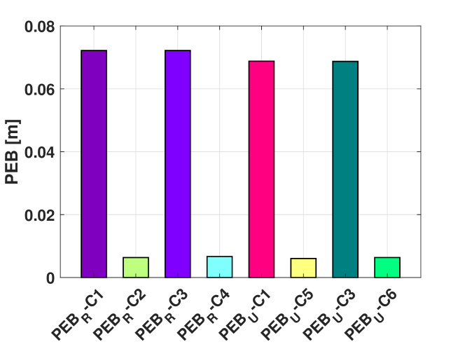
Figure 4: The role HRIS position estimation on the UE positioning accuracy, and vice versa. The HRIS common power splitting factor and the BS transmit power were set to $\rho=0.5$ and $P_{\text{B}}=15~{}\text{dBm}$, respectively.

(a)

(b)

Figure 5: The effect of the HRIS common power splitting ration $\rho$ on the estimation performance when the BS transmit power is set to $P_{\text{B}}=\text{25dBm}$. (a) The effect on the position, TOA, and rotation matrix estimations; (b) The effect on the angles estimations.

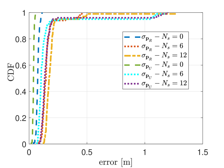
(a)

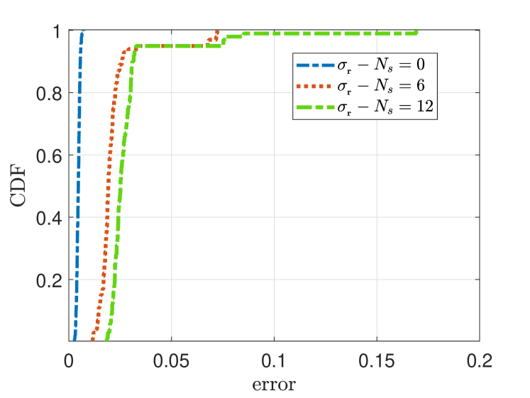
(b)

Figure 6: The evaluation of the proposed estimator for the case where SPs exist in the BS-UE and HRIS-UE links, which are randomly distributed in $[x_{0},y_{0},z_{0}]$ and $[x_{1},y_{1},z_{1}]$, with $x_{0}\sim\mathcal{U}(-8\text{m},8\text{m})$, $y_{0}\sim\mathcal{U}(0\text{m},3\text{m})$, and $z_{0}\sim\mathcal{U}(-5\text{m},1\text{m})$, as well as $x_{1}\sim\mathcal{U}(2.5\text{m},4.5\text{m})$ and $y_{1}\sim\mathcal{U}(4\text{m},11\text{m})$, $z_{1}\sim\mathcal{U}(-5\text{m},1\text{m})$. Their radar cross section is $1\text{m}^{2}$ and the HRIS common power splitting factor is set to $\rho=0.5$. (a) The effect on the estimation of the UE and HRIS positions; and (b) The effect on the estimation of $\mathbf{R}$.

V-C The Role of the HRIS Power Splitting Ratio $\rho$

We investigate the effect of $\rho$ on the estimation accuracy in Figs. 5(a) and 5(b). As previously demonstrated, the sensing/reception power at the HRIS improves with increasing $\rho$. Therefore, as it can be observed, when the value of $\rho$ increases, the corresponding CRBs of the BS-HRIS channel parameters’ estimation (i.e., $\text{ADEB}_{{}_{\text{BR}}}$, $\text{AAEB}_{{}_{\text{RB}}}$, and $\text{TEB}_{{}_{\text{BR}}}$) decline. Furthermore, we can see that the CRB of the HRIS-UE channel parameters exhibits a high error variance as $\rho$ increases. We also observe that, as $\rho$ tends to zero, the signal processed at the HRIS becomes very weak, and the error in the estimation of the BS-HRIS delay, AOD, and AOA increases. As expected, the PEB and OEB of the UE degrade as well. Conversely, when $\rho$ tends to one, the signal received by the UE via the BS-HRIS-UE link becomes very weak, and the error in the corresponding delay and AOD increases, again affecting the PEB and OEB of the UE. Therefore, there is a value of $\rho$ that minimizes the PEB and the OEB, which is not necessarily the same for both metrics. Roughly speaking a value around $\rho=0.5$ leads to a reasonable performance trade-off; similarly has been observed for full channel state information estimation [42].

V-D The Impact of SPs on the Estimation Performance

We finally investigate the robustness of the proposed estimation approach in the presence of additional SPs in the wireless environment. Figures 6(a) and 6(b) illustrate the estimation error of the state parameters for $20$ realizations of the SP positions. Without loss of generality, we set $N_{s_{0}}=N_{s_{1}}$, and we use the notation $N_{s}\triangleq N_{s_{0}}+N_{s_{1}}$. The SPs in the BS-UE link are randomly distributed in the channel environment with coordinates $[x_{0},y_{0},z_{0}]$, where $x_{0}\sim\mathcal{U}(-8\text{m},8\text{m})$, $y_{0}\sim\mathcal{U}(0\text{m},3\text{m})$, and $z_{0}\sim\mathcal{U}(-5\text{m},1\text{m})$. Similarly, the SPs in the HRIS-UE link are placed randomly in the environment with coordinates $[x_{1},y_{1},z_{1}]$, where $x_{1}\sim\mathcal{U}(2.5\text{m},4.5\text{m})$, $y_{1}\sim\mathcal{U}(4\text{m},11\text{m})$, and $z_{1}\sim\mathcal{U}(-5\text{m},1\text{m})$. We model the channel gain for the SPs according to the radar equation [59], considering that the radar cross-section is $1\mathrm{m}^{2}$. As can be seen from both figures, the interference from the SPs deteriorates the estimation accuracy. It is shown that this accuracy degrades as the number $N_{s}$ of SPs increases. Interestingly, it is depicted that the proposed estimation performs satisfactorily even in the presence of a large number of SPs, but is affected by a small number of relatively large outliers.

VI Conclusions

In this paper, we presented a multi-stage estimator for the unknown 3D rotation matrix and 3D position of a single-RX-RF HRIS and the unknown 3D position of a single-antenna UE in a multi-carrier system with a multi-antenna BS. The proposed estimation approach exploits the geometrical channel features to effectively estimate the unknown state parameters. Our simulation results confirmed the validity of the presented approach and showcased that the RMSE of the estimations attains the corresponding CRBs within a certain transmit power range. Moreover, it was demonstrated that the hris power splitting ratio between the reflecting and sensing operations of the hybrid meta-atoms plays a critical role on the overall estimation accuracy. It was finally demonstrated that the proposed joint 3D user and 6D HRIS localization method is robust enough when additional SP are present in the wireless propagation environment under investigation.

Appendix A Derivation of $\mathbf{J}_{\boldsymbol{\zeta}}$

To calculate $\mathbf{J}_{\boldsymbol{\zeta}}$ in (13), we need to compute $\partial\boldsymbol{\mu}_{{}_{t},_{k}}/\partial\boldsymbol{\zeta}=\left[{\partial[\boldsymbol{\mu}_{{}_{\text{R}},_{t}}]_{k}}/{\partial\boldsymbol{\zeta}},{\partial[\boldsymbol{\mu}_{{}_{\text{U}},_{t}}]_{k}}/{\partial\boldsymbol{\zeta}}\right]^{\top}\in\mathbb{C}^{17}$. By considering the noise-free parts of the observations at the HRIS and the UE, as given by (5) and (6), we can derive the following expressions:

$$\frac{\partial[\boldsymbol{\mu}_{{}_{\text{R}},_{t}}]_{k}}{\partial{\tau_{{}_{\text{BR}}}}} =g_{{}_{\text{BR}}}\sqrt{\rho P_{\text{B}}}[\mathbf{\dot{d}}(\tau_{{}_{\text{BR}}})]_{k}\mathbf{c}_{{}_{t}}^{\top}\mathbf{a}_{{}_{\text{R}}}(\boldsymbol{\phi}_{{}_{\text{RB}}})\mathbf{a}^{\top}_{{}_{\text{B}}}(\boldsymbol{\theta}_{{}_{\text{BR}}})\mathbf{f}_{{}_{t}},$$ (52a)

$$\frac{\partial[\boldsymbol{\mu}_{{}_{\text{U}},_{t}}]_{k}}{\partial{\tau_{{}_{\text{BR}}}}} =0,\quad\frac{\partial[\boldsymbol{\mu}_{{}_{\text{R}},_{t}}]_{k}}{\partial{\tau_{{}_{\text{BU}}}}}=0,\quad\frac{\partial[\boldsymbol{\mu}_{{}_{\text{R}},_{t}}]_{k}}{\partial{\tau_{{}_{\text{BRU}}}}}=0,$$ (52b)

$$\frac{\partial[\boldsymbol{\mu}_{{}_{\text{U}},_{t}}]_{k}}{\partial{\tau_{{}_{\text{BU}}}}} =g_{{}_{\text{BU}}}\sqrt{P_{\text{B}}}[\mathbf{\dot{d}}(\,\tau_{{}_{\text{BU}}})\,]_{{}_{k}}\mathbf{a}^{\top}_{{}_{\text{B}}}(\,\boldsymbol{\theta}_{{}_{\text{BU}}})\,\mathbf{f}_{{}_{t}},$$ (52c)

$$\frac{\partial[\boldsymbol{\mu}_{{}_{\text{U}},_{t}}]_{k}}{\partial{\tau_{{}_{\text{BRU}}}}}= g_{{}_{\text{BRU}}}\sqrt{(\,1-\rho)\,P_{\text{B}}}[\mathbf{\dot{d}}(\,\tau_{{}_{\text{BRU}}})\,]_{k}\mathbf{a}_{{}_{\text{R}}}^{\top}(\,\boldsymbol{\theta}_{{}_{\text{RU}}})\,$$

$$\text{diag}(\,\boldsymbol{\gamma}_{{}_{t}})\,\mathbf{a}_{{}_{\text{R}}}(\,\boldsymbol{\phi}_{{}_{\text{RB}}})\,\mathbf{a}^{\top}_{{}_{\text{B}}}(\,\boldsymbol{\theta}_{{}_{\text{BR}}})\,\mathbf{f}_{{}_{t}},$$ (52d)

$$\frac{\partial[\boldsymbol{\mu}_{{}_{\text{R}},_{t}}]_{k}}{\partial{[\boldsymbol{\theta}_{{}_{\text{BR}}}}]_{{}_{i}}}= g_{{}_{\text{BR}}}\sqrt{\rho P_{\text{B}}}[\mathbf{d}(\,\tau_{{}_{\text{BR}}})\,]_{{}_{k}}\mathbf{c}_{{}_{t}}^{\top}\mathbf{a}_{{}_{\text{R}}}(\,\boldsymbol{\phi}_{{}_{\text{RB}}})\,\frac{\partial{\mathbf{a}^{\top}_{{}_{\text{B}}}(\,\boldsymbol{\theta}_{{}_{\text{BR}}})\,}}{\partial{[\boldsymbol{\theta}_{{}_{\text{BR}}}}]_{{}_{i}}}\mathbf{f}_{{}_{t}}$$

$$\quad\forall i\in\{\text{el},\text{az}\},$$ (52e)

$$\frac{\partial[\boldsymbol{\mu}_{{}_{\text{U}},_{t}}]_{k}}{\partial{[\boldsymbol{\theta}_{{}_{\text{BR}}}]_{{}_{i}}}} =g_{{}_{\text{BRU}}}\sqrt{(\,1-\rho)\,P_{\text{B}}}[\mathbf{d}(\,\tau_{{}_{\text{BRU}}})\,]_{k}\mathbf{a}_{{}_{\text{R}}}^{\top}(\,\boldsymbol{\theta}_{{}_{\text{RU}}})\,\text{diag}(\,\boldsymbol{\gamma}_{{}_{t}})\,$$

$$\mathbf{a}_{{}_{\text{R}}}(\,\boldsymbol{\phi}_{{}_{\text{RB}}})\,\frac{\partial{\mathbf{a}^{\top}_{{}_{\text{B}}}(\,\boldsymbol{\theta}_{{}_{\text{BR}}})\,}}{\partial{[\boldsymbol{\theta}_{{}_{\text{BR}}}]_{{}_{i}}}}\mathbf{f}_{{}_{t}}\quad\forall i\in\{\text{el},\text{az}\},$$ (52f)

$$\frac{\partial[\boldsymbol{\mu}_{{}_{\text{R}},_{t}}]_{k}}{\partial{\boldsymbol{\boldsymbol{\theta}}_{{}_{\text{BU}}}}} =\mathbf{0}^{\top}_{2},\quad\text{and}\quad\frac{\partial[\boldsymbol{\mu}_{{}_{\text{R}},_{t}}]_{k}}{\partial{\boldsymbol{\theta}_{{}_{\text{RU}}}}}=\mathbf{0}^{\top}_{2},$$ (52g)

$$\frac{\partial[\boldsymbol{\mu}_{{}_{\text{U}},_{t}}]_{k}}{\partial{[\boldsymbol{\theta}_{{}_{\text{BU}}}]_{{}_{i}}}} =g_{{}_{\text{BU}}}\sqrt{P_{\text{B}}}[\mathbf{d}(\,\tau_{{}_{\text{BU}}})\,]_{{}_{k}}\frac{\partial{\mathbf{a}^{\top}_{{}_{\text{B}}}}(\,\boldsymbol{\theta}_{{}_{\text{BU}}})\,}{\partial{[\boldsymbol{\theta}_{{}_{\text{BU}}}]_{{}_{i}}}}\mathbf{f}_{{}_{t}}\quad\forall i\in\{\text{el},\text{az}\},$$ (52h)

$$\frac{\partial[\boldsymbol{\mu}_{{}_{\text{U}},_{t}}]_{k}}{\partial{[\boldsymbol{\theta}_{{}_{\text{RU}}}]_{{}_{i}}}}= g_{{}_{\text{BRU}}}\sqrt{(\,1-\rho)\,P_{\text{B}}}[\mathbf{d}(\,\tau_{{}_{\text{BRU}}})\,]_{k}\frac{\partial{\mathbf{a}^{\top}_{{}_{\text{R}}}(\,{\boldsymbol{\theta}}_{{}_{\text{RU}}})}}{\partial{[\boldsymbol{\theta}_{{}_{\text{RU}}}]_{{}_{i}}}}\,\text{diag}(\,\boldsymbol{\gamma}_{{}_{t}})\,$$

$$\mathbf{a}_{{}_{\text{R}}}(\,\boldsymbol{\phi}_{{}_{\text{RB}}})\,\mathbf{a}^{\top}_{{}_{\text{B}}}(\,\boldsymbol{\theta}_{{}_{\text{BR}}})\,\mathbf{f}_{{}_{t}}\quad\forall i\in\{\text{el},\text{az}\},$$ (52i)

$$\frac{\partial[\boldsymbol{\mu}_{{}_{\text{R}},_{t}}]_{k}}{\partial{[\boldsymbol{\phi}_{{}_{\text{RB}}}]_{{}_{i}}}}= g_{{}_{\text{BR}}}\sqrt{\rho P_{\text{B}}}[\mathbf{d}(\,\tau_{{}_{\text{BR}}})\,]_{{}_{k}}\mathbf{c}_{{}_{t}}^{\top}\frac{\partial\mathbf{a}_{{}_{\text{R}}}(\,\boldsymbol{\phi}_{{}_{\text{RB}}})\,}{\partial{[\boldsymbol{\phi}_{{}_{\text{RB}}}]_{{}_{i}}}}\mathbf{a}^{\top}_{{}_{\text{B}}}(\,\boldsymbol{\theta}_{{}_{\text{BR}}})\,\mathbf{f}_{{}_{t}}$$

$$\quad\forall i\in\{\text{el},\text{az}\},$$ (52j)

$$\frac{\partial[\boldsymbol{\mu}_{{}_{\text{U}},_{t}}]_{k}}{\partial{[\boldsymbol{\phi}_{{}_{\text{RB}}}}]_{{}_{i}}}= g_{{}_{\text{BRU}}}\sqrt{(\,1-\rho)\,P_{\text{B}}}[\mathbf{d}(\,\tau_{{}_{\text{BRU}}})\,]_{k}\mathbf{a}^{\top}_{{}_{\text{R}}}(\,\boldsymbol{\theta}_{{}_{\text{RU}}})\,\text{diag}(\,\boldsymbol{\gamma}_{{}_{t}})\,$$

$$\frac{\partial\mathbf{a}_{{}_{\text{R}}}(\,\boldsymbol{\phi}_{{}_{\text{RB}}})\,}{\partial{[\boldsymbol{\phi}_{{}_{\text{RB}}}}]_{{}_{i}}}\mathbf{a}^{\top}_{{}_{\text{B}}}(\,\boldsymbol{\theta}_{{}_{\text{BR}}})\,\mathbf{f}_{{}_{t}}\quad\forall i\in\{\text{el},\text{az}\},$$ (52k)

$$\frac{\partial[\boldsymbol{\mu}_{{}_{\text{R}},_{t}}]_{k}}{\partial{\mathbf{g}_{{}_{\text{BR}}}}}= \mathbf{e}^{\top}\otimes\sqrt{\rho P_{\text{B}}}[\mathbf{d}(\,\tau_{{}_{\text{BR}}})\,]_{{}_{k}}\mathbf{c}_{{}_{t}}^{\top}\mathbf{a}_{{}_{\text{R}}}(\,\boldsymbol{\phi}_{{}_{\text{RB}}})\,\mathbf{a}^{\top}_{{}_{\text{B}}}(\,\boldsymbol{\theta}_{{}_{\text{BR}}})\,\mathbf{f}_{{}_{t}},$$ (52l)

$$\frac{\partial[\boldsymbol{\mu}_{{}_{\text{U}},_{t}}]_{k}}{\partial{\mathbf{g}_{{}_{\text{BR}}}}} =\mathbf{0}_{{}_{2}}^{\top},\frac{\partial[\boldsymbol{\mu}_{{}_{\text{R}},_{t}}]_{k}}{\partial{\mathbf{g}_{{}_{\text{BU}}}}}=\mathbf{0}_{{}_{2}}^{\top},\frac{\partial[\boldsymbol{\mu}_{{}_{\text{R}},_{t}}]_{k}}{\partial{\mathbf{g}_{{}_{\text{BU}}}}}=\mathbf{0}_{{}_{2}}^{\top},$$ (52m)

$$\frac{\partial[\boldsymbol{\mu}_{{}_{\text{U}},_{t}}]_{k}}{\partial{\mathbf{g}_{{}_{\text{BU}}}}} =\mathbf{e}^{\top}\otimes\sqrt{\rho P_{\text{B}}}[\mathbf{d}(\,\tau_{{}_{\text{BU}}})\,]_{{}_{k}}\mathbf{a}^{\top}_{{}_{\text{B}}}(\,\boldsymbol{\theta}_{{}_{\text{BU}}})\,\mathbf{f}_{{}_{t}},$$ (52n)

$$\frac{\partial[\boldsymbol{\mu}_{{}_{\text{U}},_{t}}]_{k}}{\partial\mathbf{g}_{{}_{\text{BRU}}}}= \mathbf{e}^{\top}\otimes\sqrt{(\,1-\rho)\,P_{\text{B}}}[\mathbf{d}(\,\tau_{{}_{\text{BRU}}})\,]_{k}\mathbf{a}^{\top}_{{}_{\text{R}}}(\,\boldsymbol{\theta}_{{}_{\text{RU}}})\,\text{diag}(\,\boldsymbol{\gamma}_{{}_{t}})\,$$

$$\mathbf{a}_{{}_{\text{R}}}(\,\boldsymbol{\phi}_{{}_{\text{RB}}})\,\mathbf{a}_{{}_{\text{B}}}^{\top}(\,\boldsymbol{\theta}_{{}_{\text{BR}}})\,\mathbf{f}_{{}_{t}},$$ (52o)

where $\mathbf{\dot{d}}(\,\tau)\,\triangleq-\jmath 2\pi\Delta_{f}[0,\dots,k-1]^{\top}\odot\mathbf{d}(\,\tau)\,$, $\mathbf{e}\triangleq[1,\jmath]^{\top}$, and $\forall i\in\{\text{el},\text{az}\}$:

$$\allowdisplaybreaks\frac{\partial\mathbf{a}(\,\boldsymbol{\psi})\,}{\partial[\boldsymbol{\psi}]_{{}_{i}}} =\frac{\partial\mathbf{a}_{r}(\boldsymbol{\psi})}{\partial[\boldsymbol{\psi}]_{{}_{i}}}\otimes\mathbf{a}_{c}(\boldsymbol{\psi})+\mathbf{a}_{r}(\boldsymbol{\psi})\otimes\frac{\partial\mathbf{a}_{c}(\boldsymbol{\psi})}{\partial[\boldsymbol{\psi}]_{{}_{i}}}.$$ (53)

By using (11a) and (11b), and the notation $\mathbf{m}\triangleq[-(M-1)/2,\dots,(M-1)/2]^{\top}$ with $M\in\{M_{{}_{\text{B}}},M_{{}_{\text{R}}}\}$, we can write:

$$\frac{\partial\mathbf{a}_{r}(\boldsymbol{\psi})}{\partial[\boldsymbol{\psi}]_{{}_{\text{el}}}} =-\jmath\frac{2\pi d}{\lambda}\cos{[\boldsymbol{\psi}]_{\text{el}}}\cos{[\boldsymbol{\psi}]_{\text{az}}}\mathbf{m}\odot\mathbf{a}_{r}(\boldsymbol{\psi}),$$ (54a)

$$\frac{\partial\mathbf{a}_{r}(\boldsymbol{\psi})}{\partial[\boldsymbol{\psi}]_{{}_{\text{az}}}} =\jmath\frac{2\pi d}{\lambda}\sin{[\boldsymbol{\psi}]_{\text{el}}}\sin{[\boldsymbol{\psi}]_{\text{az}}}\mathbf{m}\odot\mathbf{a}_{r}(\boldsymbol{\psi}),$$ (54b)

$$\frac{\partial\mathbf{a}_{c}(\boldsymbol{\psi})}{\partial[\boldsymbol{\psi}]_{{}_{\text{el}}}} =\jmath\frac{2\pi d}{\lambda}\sin{[\boldsymbol{\psi}]_{\text{el}}}\mathbf{m}\odot\mathbf{a}_{c}(\boldsymbol{\psi}),$$ (54c)

$$\frac{\partial\mathbf{a}_{c}(\boldsymbol{\psi})}{\partial[\boldsymbol{\psi}]_{{}_{\text{az}}}} =\mathbf{0}_{{}_{M}}.$$ (54d)

Appendix B Derivation of $\mathbf{T}$

Using (8a) and  (8b), the elements of $\mathbf{T}$ are computed as:

$$\mathbf{T}(1,1:3) =\frac{\partial\tau_{{}_{\text{BR}}}}{\partial\mathbf{p}_{\text{R}}}=\frac{\mathbf{p}_{\text{R}}-\mathbf{p}_{\text{B}}}{c\|\mathbf{p}_{\text{B}}-\mathbf{p}_{\text{R}}\|},$$ (55a)

$$\mathbf{T}(1,7) =\frac{\partial\tau_{{}_{\text{BR}}}}{\partial b_{\text{R}}}=1,\quad\text{and}\quad\mathbf{T}(2,8)=\frac{\partial\tau_{{}_{\text{BU}}}}{\partial b_{\text{U}}}=1,$$ (55b)

$$\mathbf{T}(2,4:6) =\frac{\partial\tau_{{}_{\text{BU}}}}{\partial\mathbf{p}_{\text{U}}}=\frac{\mathbf{p}_{\text{U}}-\mathbf{p}_{\text{B}}}{c\|\mathbf{p}_{\text{B}}-\mathbf{p}_{\text{U}}\|},$$ (55c)

$$\mathbf{T}(3,1:3) =\frac{\partial\tau_{{}_{\text{BRU}}}}{\partial\mathbf{p}_{\text{R}}}=\frac{\mathbf{p}_{\text{R}}-\mathbf{p}_{\text{B}}}{c\|\mathbf{p}_{\text{B}}-\mathbf{p}_{\text{R}}\|},$$ (55d)

$$\mathbf{T}(3,4:6) =\frac{\partial\tau_{{}_{\text{BRU}}}}{\partial\mathbf{p}_{\text{U}}}=\frac{\mathbf{p}_{\text{U}}-\mathbf{p}_{\text{B}}}{c\|\mathbf{p}_{\text{B}}-\mathbf{p}_{\text{U}}\|},$$ (55e)

$$\mathbf{T}(3,7:8) =\Big{[}\,\frac{\partial\tau_{{}_{\text{BRU}}}}{\partial b_{\text{R}}},\frac{\partial\tau_{{}_{\text{BRU}}}}{\partial b_{\text{U}}}\Big{]}\,=[1,1].$$ (55f)

To derive the derivatives of the AOAs and AODs w.r.t. state parameters, we first introduce the following auxiliary variables:

$$\mathbf{u}_{{}_{\text{DR}}}\triangleq\frac{\mathbf{p}_{\text{R}}-\mathbf{p}_{\text{B}}}{\|\mathbf{p}_{\text{R}}-\mathbf{p}_{\text{B}}\|}\quad\text{and }\quad\mathbf{u}_{{}_{\text{DU}}}\triangleq\frac{\mathbf{p}_{\text{U}}-\mathbf{p}_{\text{B}}}{\|\mathbf{p}_{\text{U}}-\mathbf{p}_{\text{B}}\|},$$ (56a)

$$\mathbf{v}_{{}_{\text{AB}}}\triangleq\frac{\mathbf{p}_{\text{B}}-\mathbf{p}_{\text{R}}}{\|\mathbf{p}_{\text{B}}-\mathbf{p}_{\text{R}}\|}\quad\text{and }\quad\mathbf{v}_{{}_{\text{DU}}}\triangleq\frac{\mathbf{p}_{\text{U}}-\mathbf{p}_{\text{R}}}{\|\mathbf{p}_{\text{U}}-\mathbf{p}_{\text{R}}\|},$$ (56b)

as well as $\mathbf{u}_{{}_{1}}\triangleq[1,0,0]^{\top}$, $\mathbf{u}_{{}_{2}}\triangleq[0,1,0]^{\top}$, and $\mathbf{u}_{{}_{3}}\triangleq[0,0,1]^{\top}$. Then, we may rewrite the AOAs and AODs as follows [60, Appendix A]:

$$\boldsymbol{\theta}_{{}_{\text{BR}}} =[{\theta}_{{}_{\text{BR}}}^{(\text{az})},{\theta}_{{}_{\text{BR}}}^{(\text{el})}]^{\top}=[\text{atan2}(\mathbf{u}_{2}^{\top}\mathbf{u}_{{}_{\text{DR}}},\mathbf{u}_{1}^{\top}\mathbf{u}_{{}_{\text{DR}}}),\text{acos}(\mathbf{u}_{3}^{\top}\mathbf{u}_{{}_{\text{DR}}})]^{\top},$$ (57a)

$$\boldsymbol{\theta}_{{}_{\text{BU}}} =[{\theta}_{{}_{\text{BU}}}^{(\text{az})},{\theta}_{{}_{\text{BU}}}^{(\text{el})}]^{\top}=[\text{atan2}(\mathbf{u}_{2}^{\top}\mathbf{u}_{{}_{\text{DU}}},\mathbf{u}_{1}^{\top}\mathbf{u}_{{}_{\text{DU}}}),\text{acos}(\mathbf{u}_{3}^{\top}\mathbf{u}_{{}_{\text{DR}}})]^{\top},$$ (57b)

$$\boldsymbol{\phi}_{{}_{\text{RB}}} =[{\phi}_{{}_{\text{RB}}}^{(\text{az})},{\phi}_{{}_{\text{RB}}}^{(\text{el})}]^{\top}=[\text{atan2}(\mathbf{r}_{2}^{\top}\mathbf{v}_{{}_{\text{AB}}}),\mathbf{r}_{1}^{\top}\mathbf{v}_{{}_{\text{AB}}})),\text{acos}(\mathbf{r}_{2}^{\top}\mathbf{v}_{{}_{\text{AB}}})]^{\top},$$ (57c)

$$\boldsymbol{\theta}_{{}_{\text{RU}}} =[{\theta}_{{}_{\text{RU}}}^{(\text{az})},{\theta}_{{}_{\text{RU}}}^{(\text{el})}]^{\top}=[\text{atan2}(\mathbf{r}_{2}^{\top}\mathbf{v}_{{}_{\text{DU}}},\mathbf{r}_{1}^{\top}\mathbf{v}_{{}_{\text{DU}}}),\text{acos}(\mathbf{r}_{3}^{\top}\mathbf{v}_{{}_{\text{DU}}})]^{\top},$$ (57d)

yielding the following derivatives:

$$\frac{\partial\mathbf{u}_{{}_{\text{DR}}}}{\partial\mathbf{p}_{\text{R}}} =(\,\mathbf{I}_{3}-\mathbf{u}_{{}_{\text{DR}}}\mathbf{u}_{{}_{\text{DR}}}^{\top})\,/\|\mathbf{p}_{\text{B}}-\mathbf{p}_{\text{R}}\|\quad,$$ (58a)

$$\frac{\partial\mathbf{u}_{{}_{\text{DU}}}}{\partial\mathbf{p}_{\text{U}}} =(\,\mathbf{I}_{3}-\mathbf{u}_{{}_{\text{DU}}}\mathbf{u}_{{}_{\text{DU}}}^{\top})\,/\|\mathbf{p}_{\text{B}}-\mathbf{p}_{\text{U}}\|\quad,$$ (58b)

$$\frac{\partial\mathbf{v}_{{}_{\text{AB}}}}{\partial\mathbf{p}_{\text{R}}} =(\,\mathbf{v}_{{}_{\text{AB}}}\mathbf{v}_{{}_{\text{AB}}}^{\top}-\mathbf{I}_{3})\,/\|\mathbf{p}_{\text{B}}-\mathbf{p}_{\text{R}}\|\quad,$$ (58c)

$$\frac{\partial\mathbf{v}_{{}_{\text{DU}}}}{\partial\mathbf{p}_{\text{R}}} =(\,\mathbf{v}_{{}_{\text{DU}}}\mathbf{v}_{{}_{\text{DU}}}^{\top}-\mathbf{I}_{3})\,/\|\mathbf{p}_{\text{U}}-\mathbf{p}_{\text{R}}\|\quad,$$ (58d)

$$\frac{\partial\mathbf{v}_{{}_{\text{DU}}}}{\partial\mathbf{p}_{\text{U}}} =(\,\mathbf{I}_{3}-\mathbf{v}_{{}_{\text{DU}}}\mathbf{v}_{{}_{\text{DU}}}^{\top})\,/\|\mathbf{p}_{\text{U}}-\mathbf{p}_{\text{R}}\|\quad,$$ (58e)

$$\frac{\partial{\theta}_{{}_{\text{BR}}}^{(\text{az})}}{\partial\mathbf{u}_{{}_{\text{DR}}}} =\frac{(\,\mathbf{u}_{1}^{\top}\mathbf{u}_{{}_{\text{DR}}})\,\mathbf{u}_{2}-(\,\mathbf{u}_{2}^{\top}\mathbf{u}_{{}_{\text{DR}}})\,\mathbf{u}_{1}}{(\,\mathbf{u}_{1}^{\top}\mathbf{u}_{{}_{\text{DR}}})\,^{2}+(\,\mathbf{u}_{2}^{\top}\mathbf{u}_{{}_{\text{DR}}})\,^{2}}\quad,$$ (58f)

$$\frac{\partial{\theta}_{{}_{\text{BR}}}^{(\text{el})}}{\partial\mathbf{u}_{{}_{\text{DR}}}} =-\frac{\mathbf{u}_{3}}{\sqrt{1-(\mathbf{u}_{3}^{\top}\mathbf{u}_{{}_{\text{DR}}})^{2}}}\quad,$$ (58g)

$$\frac{\partial{\theta}_{{}_{\text{BU}}}^{(\text{az})}}{\partial\mathbf{u}_{{}_{\text{DR}}}} =\frac{(\,\mathbf{u}_{1}^{\top}\mathbf{u}_{{}_{\text{DR}}})\,\mathbf{u}_{2}-(\,\mathbf{u}_{2}^{\top}\mathbf{u}_{{}_{\text{DR}}})\,\mathbf{u}_{1}}{(\,\mathbf{u}_{1}^{\top}\mathbf{u}_{{}_{\text{DR}}})\,^{2}+(\,\mathbf{u}_{2}^{\top}\mathbf{u}_{{}_{\text{DR}}})\,^{2}}\quad,$$ (58h)

$$\frac{\partial{\theta}_{{}_{\text{BU}}}^{(\text{el})}}{\partial\mathbf{u}_{{}_{\text{DR}}}} =-\frac{\mathbf{u}_{3}}{\sqrt{1-(\mathbf{u}_{3}^{\top}\mathbf{u}_{{}_{\text{DR}}})^{2}}}\quad,$$ (58i)

$$\frac{\partial{\theta}_{{}_{\text{RU}}}^{(\text{az})}}{\partial\mathbf{v}_{{}_{\text{DU}}}} =\frac{(\,\mathbf{r}_{1}^{\top}\mathbf{v}_{{}_{\text{DU}}})\,\mathbf{r}_{2}-(\,\mathbf{r}_{2}^{\top}\mathbf{v}_{{}_{\text{DU}}})\,\mathbf{r}_{1}}{(\,\mathbf{r}_{1}^{\top}\mathbf{v}_{{}_{\text{DU}}})\,^{2}+(\,\mathbf{r}_{2}^{\top}\mathbf{v}_{{}_{\text{DU}}})\,^{2}}\quad,$$ (58j)

$$\frac{\partial{\theta}_{{}_{\text{RU}}}^{(\text{el})}}{\partial\mathbf{v}_{{}_{\text{DU}}}} =-\frac{\mathbf{r}_{3}}{\sqrt{1-(\mathbf{r}_{3}^{\top}\mathbf{v}_{{}_{\text{DU}}})^{2}}}\quad,$$ (58k)

$$\frac{\partial{\phi}_{{}_{\text{RB}}}^{(\text{az})}}{\partial\mathbf{v}_{{}_{\text{AB}}}} =\frac{(\,\mathbf{r}_{1}^{\top}\mathbf{v}_{{}_{\text{AB}}})\,\mathbf{r}_{2}-(\,\mathbf{r}_{2}^{\top}\mathbf{v}_{{}_{\text{AB}}})\,\mathbf{r}_{1}}{(\,\mathbf{r}_{1}^{\top}\mathbf{v}_{{}_{\text{AB}}})\,^{2}+(\,\mathbf{r}_{2}^{\top}\mathbf{v}_{{}_{\text{AB}}})\,^{2}}\quad,$$ (58l)

$$\frac{\partial{\phi}_{{}_{\text{RB}}}^{(\text{el})}}{\partial\mathbf{v}_{{}_{\text{AB}}}} =-\frac{\mathbf{r}_{3}}{\sqrt{1-(\mathbf{r}_{3}^{\top}\mathbf{v}_{{}_{\text{AB}}})^{2}}}\quad,$$ (58m)

$$\frac{\partial{\phi}_{{}_{\text{RB}}}^{(\text{az})}}{\partial\mathbf{R}} =\frac{(\,\mathbf{r}_{1}^{\top}\mathbf{v}_{{}_{\text{AB}}})\,\mathbf{v}_{{}_{\text{AB}}}\mathbf{u}_{2}^{\top}-(\,\mathbf{r}_{2}^{\top}\mathbf{v}_{{}_{\text{AB}}})\,\mathbf{v}_{{}_{\text{AB}}}\mathbf{u}_{1}^{\top}}{(\,\mathbf{r}_{1}^{\top}\mathbf{v}_{{}_{\text{AB}}})\,^{2}+(\,\mathbf{r}_{2}^{\top}\mathbf{v}_{{}_{\text{AB}}})\,^{2}}\quad,$$ (58n)

$$\frac{\partial{\phi}_{{}_{\text{RB}}}^{(\text{el})}}{\partial\mathbf{R}} =-\frac{\mathbf{v}_{{}_{\text{AB}}}\mathbf{u}_{3}^{\top}}{\sqrt{1-(\mathbf{r}_{3}^{\top}\mathbf{v}_{{}_{\text{AB}}})^{2}}}\quad,$$ (58o)

$$\frac{\partial{\theta}_{{}_{\text{RU}}}^{(\text{az})}}{\partial\mathbf{R}} =\frac{(\,\mathbf{r}_{1}^{\top}\mathbf{v}_{{}_{\text{DU}}})\,\mathbf{v}_{{}_{\text{DU}}}\mathbf{u}_{2}^{\top}-(\,\mathbf{r}_{2}^{\top}\mathbf{v}_{{}_{\text{DU}}})\,\mathbf{v}_{{}_{\text{DU}}}\mathbf{u}_{1}^{\top}}{(\,\mathbf{r}_{1}^{\top}\mathbf{v}_{{}_{\text{DU}}})\,^{2}+(\,\mathbf{r}_{2}^{\top}\mathbf{v}_{{}_{\text{DU}}})\,^{2}}\quad,$$ (58p)

$$\frac{\partial{\theta}_{{}_{\text{RU}}}^{(\text{el})}}{\partial\mathbf{R}} =-\frac{\mathbf{v}_{{}_{\text{DU}}}\mathbf{u}_{3}^{\top}}{\sqrt{1-(\mathbf{r}_{3}^{\top}\mathbf{v}_{{}_{\text{DU}}})^{2}}}\quad,$$ (58q)

The latter expressions are used to compute the following elements of $\mathbf{T}$ (with those remaining being zero):

$$\mathbf{T}(4,1:3) =\frac{\partial\theta_{{}_{\text{BR}}}^{(\text{az})}}{\partial\mathbf{p}_{\text{R}}}=\frac{\partial\theta_{{}_{\text{BR}}}^{(\text{az})}}{\partial\mathbf{u}_{{}_{\text{DR}}}}\frac{\partial\mathbf{u}_{{}_{\text{DR}}}}{\partial\mathbf{p}_{\text{R}}},$$ (59a)

$$\mathbf{T}(5,1:3) =\frac{\partial\theta_{{}_{\text{BR}}}^{(\text{el})}}{\partial\mathbf{p}_{\text{R}}}=\frac{\partial\theta_{{}_{\text{BR}}}^{(\text{el})}}{\partial\mathbf{u}_{{}_{\text{DR}}}}\frac{\partial\mathbf{u}_{{}_{\text{DR}}}}{\partial\mathbf{p}_{\text{R}}},$$ (59b)

$$\mathbf{T}(6,4:6) =\frac{\partial\theta_{{}_{\text{BU}}}^{(\text{az})}}{\partial\mathbf{p}_{\text{U}}}=\frac{\partial\theta_{{}_{\text{BU}}}^{(\text{az})}}{\partial\mathbf{u}_{{}_{\text{DU}}}}\frac{\partial\mathbf{u}_{{}_{\text{DU}}}}{\partial\mathbf{p}_{\text{U}}},$$ (59c)

$$\mathbf{T}(7,4:6) =\frac{\partial\theta_{{}_{\text{BU}}}^{(\text{el})}}{\partial\mathbf{p}_{\text{U}}}=\frac{\partial\theta_{{}_{\text{BU}}}^{(\text{el})}}{\partial\mathbf{u}_{{}_{\text{DU}}}}\frac{\partial\mathbf{u}_{{}_{\text{DU}}}}{\partial\mathbf{p}_{\text{U}}},$$ (59d)

$$\mathbf{T}(8,1:3) =\frac{\partial\theta_{{}_{\text{RU}}}^{(\text{az})}}{\partial\mathbf{p}_{\text{R}}}=\frac{\partial\theta_{{}_{\text{RU}}}^{(\text{az})}}{\partial\mathbf{v}_{{}_{\text{DU}}}}\frac{\partial\mathbf{v}_{{}_{\text{DU}}}}{\partial\mathbf{p}_{\text{R}}},$$ (59e)

$$\mathbf{T}(9,1:3) =\frac{\partial\theta_{{}_{\text{RU}}}^{(\text{el})}}{\partial\mathbf{p}_{\text{R}}}=\frac{\partial\theta_{{}_{\text{RU}}}^{(\text{el})}}{\partial\mathbf{v}_{{}_{\text{DU}}}}\frac{\partial\mathbf{v}_{{}_{\text{DU}}}}{\partial\mathbf{p}_{\text{R}}},$$ (59f)

$$\mathbf{T}(8,4:6) =\frac{\partial\theta_{{}_{\text{RU}}}^{(\text{az})}}{\partial\mathbf{p}_{\text{U}}}=\frac{\partial\theta_{{}_{\text{RU}}}^{(\text{az})}}{\partial\mathbf{v}_{{}_{\text{DU}}}}\frac{\partial\mathbf{v}_{{}_{\text{DU}}}}{\partial\mathbf{p}_{\text{U}}},$$ (59g)

$$\mathbf{T}(9,4:6) =\frac{\partial\theta_{{}_{\text{RU}}}^{(\text{el})}}{\partial\mathbf{p}_{\text{U}}}=\frac{\partial\theta_{{}_{\text{RU}}}^{(\text{el})}}{\partial\mathbf{v}_{{}_{\text{DU}}}}\frac{\partial\mathbf{v}_{{}_{\text{DU}}}}{\partial\mathbf{p}_{\text{U}}},$$ (59h)

$$\mathbf{T}(10,1:3) =\frac{\partial\phi_{{}_{\text{RB}}}^{(\text{az})}}{\partial\mathbf{p}_{\text{R}}}=\frac{\partial\phi_{{}_{\text{RB}}}^{(\text{az})}}{\partial\mathbf{v}_{{}_{\text{AB}}}}\frac{\partial\mathbf{v}_{{}_{\text{AB}}}}{\partial\mathbf{p}_{\text{R}}},$$ (59i)

$$\mathbf{T}(11,1:3) =\frac{\partial\phi_{{}_{\text{RB}}}^{(\text{el})}}{\partial\mathbf{p}_{\text{R}}}=\frac{\partial\phi_{{}_{\text{RB}}}^{(\text{el})}}{\partial\mathbf{v}_{{}_{\text{AB}}}}\frac{\partial\mathbf{v}_{{}_{\text{AB}}}}{\partial\mathbf{p}_{\text{R}}},$$ (59j)

$$\mathbf{T}(8,9:17) =\frac{\partial{\theta}_{{}_{\text{RU}}}^{(\text{az})}}{\partial\mathbf{R}},\quad\text{and}\quad\mathbf{T}(9,9:17)=\frac{\partial{\theta}_{{}_{\text{RU}}}^{(\text{el})}}{\partial\mathbf{R}},$$ (59k)

$$\mathbf{T}(10,9:17) =\frac{\partial{\phi}_{{}_{\text{RB}}}^{(\text{az})}}{\partial\mathbf{R}},\quad\text{and}\quad\mathbf{T}(11,9:17)=\frac{\partial{\phi}_{{}_{\text{RB}}}^{(\text{el})}}{\partial\mathbf{R}}.$$ (59l)

References

• [1] C. Huang, A. Zappone, G. C. Alexandropoulos, M. Debbah, and C. Yuen, “Reconfigurable intelligent surfaces for energy efficiency in wireless communication,” IEEE Trans. Wireless Commun., vol. 18, no. 8, pp. 4157–4170, Aug. 2019.
• [2] M. Di Renzo, M. Debbah, D.-T. Phan-Huy, A. Zappone, M.-S. Alouini, C. Yuen, V. Sciancalepore, G. C. Alexandropoulos, J. Hoydis, H. Gacanin, J. de Rosny, A. Bounceu, G. Lerosey, and M. Fink, “Smart radio environments empowered by reconfigurable AI meta-surfaces: an idea whose time has come,” EURASIP JWCN, vol. 2019, no. 1, pp. 1–20, May 2019.
• [3] Q. Wu and R. Zhang, “Towards smart and reconfigurable environment: Intelligent reflecting surface aided wireless network,” IEEE Communications Magazine, vol. 58, no. 1, pp. 106–112, 2019.
• [4] G. C. Alexandropoulos, N. Shlezinger, and P. del Hougne, “Reconfigurable intelligent surfaces for rich scattering wireless communications: Recent experiments, challenges, and opportunities,” IEEE Commun. Mag., vol. 59, no. 6, pp. 28–34, Jun. 2021.
• [5] G. C. Alexandropoulos et al., “Reconfigurable intelligent surfaces and metamaterials: The potential of wave propagation control for 6G wireless communications,” IEEE ComSoc TCCN Newslett., vol. 6, no. 1, pp. 25–37, Jun. 2020.
• [6] Q. Li, M. Wen, S. Wang, G. C. Alexandropoulos, and Y.-C. Wu, “Space shift keying with reconfigurable intelligent surfaces: Phase configuration designs and performance analysis,” IEEE Open J. Commun. Society, vol. 2, pp. 322–333, Feb. 2021.
• [7] J. Yuan, M. Wen, Q. Li, E. Basar, G. C. Alexandropoulos, and G. Chen, “Receive quadrature reflecting modulation for RIS-empowered wireless communications,” IEEE Trans. Veh. Technol., vol. 70, no. 5, pp. 5121–5125, May 2021.
• [8] H. Wymeersch et al., “Radio localization and mapping with reconfigurable intelligent surfaces: Challenges, opportunities, and research directions,” IEEE Veh. Technol.Mag., vol. 15, no. 4, pp. 52–61, Dec. 2020.
• [9] S. P. Chepuri, N. Shlezinger, F. Liu, G. C. Alexandropoulos, S. Buzzi, and Y. C. Eldar, “Integrated sensing and communications with reconfigurable intelligent surfaces,” IEEE Signal Process. Mag., vol. 40, no. 6, pp. 41–62, Sep. 2023.
• [10] E. Calvanese Strinati, G. C. Alexandropoulos, H. Wymeersch, B. Denis, V. Sciancalepore, R. D’Errico, A. Clemente, D.-T. Phan-Huy, E. De Carvalho, and P. Popovski, “Reconfigurable, intelligent, and sustainable wireless environments for 6G smart connectivity,” IEEE Commun. Mag., vol. 59, no. 10, pp. 99–105, Oct. 2021.
• [11] G. C. Alexandropoulos, K. Stylianopoulos, C. Huang, C. Yuen, M. Bennis, and M. Debbah, “Pervasive machine learning for smart radio environments enabled by reconfigurable intelligent surfaces,” Proc. IEEE, vol. 110, no. 9, pp. 1494–1525, Sep. 2022.
• [12] W. Saad, M. Bennis, and M. Chen, “A vision of 6G wireless systems: Applications, trends, technologies, and open research pproblems,” IEEE Network, vol. 34, no. 3, pp. 134–142, May/Jun. 2019.
• [13] A. Masaracchia, D. V. Huynh, G. C. Alexandropoulos, B. Canberk, O. A. Dobre, and T. Q. Duong, “Towards the metaverse realization in 6G: Orchestration of RIS-enabled smart wireless environments via digital twins,” IEEE Internet of Things Mag., to appear, 2023.
• [14] Z. Abu Shaban, K. Keykhosravi, M. F. Keskin, G. C. Alexandropoulos, G. Seco-Granados, and H. Wymeersch, “Near-field localization with a reconfigurable intelligent surface acting as lens,” in IEEE International Conference on Communications, 2021, pp. 1–6.
• [15] K. Keykhosravi, M. F. Keskin, G. Seco-Granados, and H. Wymeersch, “SISO RIS-enabled joint 3D downlink localization and synchronization,” in IEEE International Conference on Communications, 2021, pp. 1–6.
• [16] K. Keykhosravi, M. F. Keskin, G. Seco-Granados, P. Popovski, and H. Wymeersch, “RIS-enabled SISO localization under user mobility and spatial-wideband effects,” IEEE Journal of Selected Topics in Signal Processing, 2022.
• [17] G. C. Alexandropoulos, I. Vinieratou, and H. Wymeersch, “Localization via multiple reconfigurable intelligent surfaces equipped with single receive RF chains,” IEEE Wireless Commun. Lett., vol. 11, no. 5, pp. 1072–1076, May 2022.
• [18] X. Zhang and H. Zhang, “Hybrid reconfigurable intelligent surfaces-assisted near-field localization,” IEEE Communications Letters, 2022.
• [19] C. Gaudreauand and A. Chaaban, “Localization by modulated reconfigurable intelligent surfaces,” IEEE Communications Letters, vol. 26, no. 12, pp. 2904–2908, 2022.
• [20] X. Gan, C. Huang, Z. Yang, C. Zhong, and Z. Zhang, “Near-field localization for holographic RIS assisted mmwave systems,” IEEE Communications Letters, 2022.
• [21] O. Rinchi, A. Elzanaty, and M.-S. Alouini, “Compressive near-field localization for multipath RIS-aided environments,” IEEE Communications Letters, 2022.
• [22] H. Zhang, H. Zhang, B. Di, K. Bian, Z. Han, and L. Song, “Metalocalization: Reconfigurable intelligent surface aided multi-user wireless indoor localization,” IEEE Transactions on Wireless Communications, vol. 20, no. 12, pp. 7743–7757, 2021.
• [23] G. Mylonopoulos, C. D’Andrea, and S. Buzzi, “Active reconfigurable intelligent surfaces for user localization in mmwave MIMO systems,” in IEEE 23rd International Workshop on Signal Processing Advances in Wireless Communication (SPAWC), 2022, pp. 1–5.
• [24] D. Dardari, N. Decarli, A. Guerra, and F. Guidi, “LOS/NLOS near-field localization with a large reconfigurable intelligent surface,” IEEE Transactions on Wireless Communications, 2021.
• [25] A. Elzanaty, A. Guerra, F. Guidi, and M.-S. Alouini, “Reconfigurable intelligent surfaces for localization: Position and orientation error bounds,” IEEE Transactions on Signal Processing, vol. 69, pp. 5386–5402, 2021.
• [26] R. Ghazalian, K. Keykhosravi, H. Chen, H. Wymeersch, and R. Jäntti, “Bi-static sensing for near-field RIS localization,” in IEEE Global Communications Conference, 2022, pp. 6457–6462.
• [27] R. Ghazalian, H. Chen, G. C. Alexandropoulos, G. Seco-Granados, H. Wymeersch, and R. Jäntti, “Joint user localization and location calibration of a hybrid reconfigurable intelligent surface,” IEEE Trans. Veh. Technol., to appear, 2023.
• [28] K. Keykhosravi, M. F. Keskin, S. Dwivedi, G. Seco-Granados, and H. Wymeersch, “Semi-passive 3D positioning of multiple RIS-enabled users,” IEEE Transactions on Vehicular Technology, vol. 70, no. 10, pp. 11 073–11 077, 2021.
• [29] J. He, A. Fakhreddine, H. Wymeersch, and G. C. Alexandropoulos, “Compressed-sensing-based 3D localization with distributed passive reconfigurable intelligent surfaces,” in Proc. IEEE International Conference on Acoustics, Speech, and Signal Processing, Rhodes, Greece, Jun. 2023.
• [30] K. Keykhosravi, B. Denis, G. C. Alexandropoulos, Z. S. He, A. Albanese, V. Sciancalepore, and H. Wymeersch, “Leveraging RIS-enabled smart signal propagation for solving infeasible localization problems,” IEEE Veh. Technol. Mag., early access, 2023.
• [31] C. Huang, G. C. Alexandropoulos, C. Yuen, and M. Debbah, “Indoor signal focusing with deep learning designed reconfigurable intelligent surfaces,” in Proc. IEEE SPAWC, Cannes, France, Jul. 2019.
• [32] G. C. Alexandropoulos, S. Samarakoon, M. Bennis, and M. Debbah, “Phase configuration learning in wireless networks with multiple reconfigurable intelligent surfaces,” in Proc. IEEE GLOBECOM, Taipei, Taiwan, Dec. 2020.
• [33] J. He, A. Fakhreddine, and G. C. Alexandropoulos, “STAR-RIS-enabled simultaneous indoor and outdoor 3D localization: Theoretical analysis and algorithmic estimation,” IET Signal Process., vol. 17, p. e12209, Apr. 2023.
• [34] I. Gavras, M. A. Islam, B. Smida, and G. C. Alexandropoulos, “Full duplex holographic MIMO for near-field integrated sensing and communications,” in Proc. European Signal Proces. Conf., Helsinki, Finland, Sep. 2023.
• [35] J. He, A. Fakhreddine, C. Vanwynsberghe, H. Wymeersch, and G. C. Alexandropoulos, “3D localization with a single partially-connected receiving RIS: Positioning error analysis and algorithmic design,” IEEE Trans. Veh. Technol., vol. 72, no. 10, pp. 13 190–13 202, Oct. 2023.
• [36] C. K. Sheemar, G. C. Alexandropoulos, D. Slock, J. Querol, and S. Chatzinotas, “Full-duplex-enabled joint communications and sensing with reconfigurable intelligent surfaces,” in Proc. European Signal Proces. Conf., Helsinki, Finland, Sep. 2023.
• [37] K. Stylianopoulos, M. Bayraktar, N. González-Prelcic, and G. C. Alexandropoulos, “Autoregressive attention neural networks for non-line-of-sight user tracking with dynamic metasurface antennas,” in Proc. IEEE Workshop on Computational Advances in Multi-Sensor Adaptive Processing, Los Sueños, Costa Rica, Dec. 2023.
• [38] R. Liu, M. Li, H. Luo, Q. Liu, and A. L. Swindlehurst, “Integrated sensing and communication with reconfigurable intelligent surfaces: Opportunities, applications, and future directions,” IEEE Wireless Communications, vol. 30, no. 1, pp. 50–57, 2023.
• [39] P. Chen, Z. Chen, B. Zheng, and X. Wang, “Efficient DOA estimation method for reconfigurable intelligent surfaces aided UAV swarm,” IEEE Transactions on Signal Processing, vol. 70, pp. 743–755, 2022.
• [40] J. He, A. Fakhreddine, and G. C. Alexandropoulos, “Joint channel and direction estimation for ground-to-UAV communications enabled by a simultaneous reflecting and sensing RIS,” in Proc. IEEE Int. Conf. Acoustics, Speech, and Signal Process., Rhodes, Greece, Jun. 2023.
• [41] G. C. Alexandropoulos and E. Vlachos, “A hardware architecture for reconfigurable intelligent surfaces with minimal active elements for explicit channel estimation,” in Proc. IEEE ICASSP, Barcelona, Spain, May 2020.
• [42] G. C. Alexandropoulos, N. Shlezinger, I. Alamzadeh, M. F. Imani, H. Zhang, and Y. C. Eldar, “Hybrid reconfigurable intelligent metasurfaces: Enabling simultaneous tunable reflections and sensing for 6G wireless communications,” arXiv preprint arXiv:2104.04690, 2021.
• [43] I. Alamzadeh, G. C. Alexandropoulos, N. Shlezinger, and M. F. Imani, “A reconfigurable intelligent surface with integrated sensing capability,” Scientific reports, vol. 11, no. 1, pp. 1–10, 2021.
• [44] H. Zhang, N. Shlezinger, G. C. Alexandropoulos, I. Alamzadeh, M. F. Imani, and Y. C. Eldar, “Channel estimation with hybrid reconfigurable intelligent metasurfaces,” IEEE Trans. Commun., vol. 71, no. 4, pp. 2441–2456, Apr. 2023.
• [45] Z. Liu, H. Zhang, T. Huang, F. Xu, and Y. C. Eldar, “Hybrid RIS-assisted MIMO dual-function radar-communication system,” arXiv preprint arXiv:2303.16278, 2023.
• [46] M. Jian, G. C. Alexandropoulos, E. Basar, C. Huang, R. Liu, Y. Liu, and C. Yuen, “Reconfigurable intelligent surfaces for wireless communications: Overview of hardware designs, channel models, and estimation techniques,” Int. Conv. Netw., vol. 3, no. 1, pp. 1–32, Mar. 2022.
• [47] G. C. Alexandropoulos, M. Crozzoli, D.-T. Phan-Huy, K. D. Katsanos, H. Wymeersch, P. Popovski, P. Ratajczak, Y. Bénédic, M.-H. Hamon, S. Herraiz Gonzalez, R. D’Errico, and E. Calvanese Strinati, “RIS-enabled smart wireless environments: Deployment scenarios, network architecture, bandwidth and area of influence,” EURASIP J. Wireless Commun. Netw., to appear, 2023.
• [48] S. M. Kay, Fundamentals of statistical signal processing: estimation theory.   Prentice-Hall, Inc., 1993.
• [49] E. Ollila, V. Koivunen, and J. Eriksson, “On the cramér-rao bound for the constrained and unconstrained complex parameters,” in 5th IEEE Sensor Array and Multichannel Signal Processing Workshop, 2008, pp. 414–418.
• [50] B. Mamandipoor, D. Ramasamy, and U. Madhow, “Newtonized orthogonal matching pursuit: Frequency estimation over the continuum,” IEEE Trans. Signal Process., vol. 64, no. 19, pp. 5066–5081, Oct. 2016.
• [51] Y. Han, T.-H. Hsu, C.-K. Wen, K.-K. Wong, and S. Jin, “Efficient downlink channel reconstruction for FDD multi-antenna systems,” IEEE Trans. Wireless Commun., vol. 18, no. 6, pp. 3161–3176, Jun. 2019.
• [52] M. Li, S. Zhang, F. Gao, P. Fan, and O. A. Dobre, “A new path division multiple access for the massive MIMO-OTFS networks,” IEEE J. Sel. Areas Commun., vol. 39, no. 4, pp. 903–918, Apr. 2020.
• [53] J. R. Hurley and R. B. Cattell, “The procrustes program: Producing direct rotation to test a hypothesized factor structure,” Behavioral Srucience, vol. 7, no. 2, p. 258, 1962.
• [54] P. H. Schönemann, “A generalized solution of the orthogonal procrustes problem,” Psychometrika, vol. 31, no. 1, pp. 1–10, 1966.
• [55] D. W. Eggert, A. Lorusso, and R. B. Fisher, “Estimating 3-D rigid body transformations: a comparison of four major algorithms,” Machine vision and applications, vol. 9, no. 5-6, pp. 272–290, 1997.
• [56] Y. Wang, Y. Zhang, Z. Tian, G. Leus, and G. Zhang, “Super-resolution channel estimation for arbitrary arrays in hybrid millimeter-wave massive MIMO systems,” IEEE J. Sel. Topics Signal Process., vol. 13, no. 5, pp. 947–960, 2019.
• [57] C. Ozturk, M. F. Keskin, H. Wymeersch, and S. Gezici, “Ris-aided near-field localization under phase-dependent amplitude variations,” IEEE Transactions on Wireless Communications, 2023.
• [58] S. W. Ellingson, “Path loss in reconfigurable intelligent surface-enabled channels,” in Proc. IEEE Int. Symp. Personal, Indoor and Mobile Radio Commun., 2021, pp. 829–835.
• [59] M. I. Skolnik, Introduction to radar systems.   McGraw-Hill, Inc., 1980.
• [60] M. A. Nazari, G. Seco-Granados, P. Johannisson, and H. Wymeersch, “Mmwave 6D radio localization with a snapshot observation from a single BS,” IEEE Trans. Veh. Technol., to appear, 2023.