Opto-RF transduction in Er³⁺:CaWO₄

Abstract

We use an erbium doped CaWO₄ crystal as a resonant transducer between the RF and optical domains at 12 GHz and 1532 nm respectively. We employ a RF resonator to enhance the spin coupling but keep a single-pass (non-resonant) setup in optics. The overall efficiency is low but we carefully characterize the transduction process and show that the performance can be described by two different metrics that we define and distinguish: the electro-optics and the quantum efficiencies. We reach an electro-optics efficiency of -84 dB for 15.7 dBm RF power. The corresponding quantum efficiency is -142 dB for 0.4 dBm optical power. We develop the Schrödinger-Maxwell formalism, well-known to describe light-matter interactions in atomic systems, in order to model the conversion process. We explicitly make the connection with the cavity quantum electrodynamics (cavity QED) approach that are generally used to describe quantum transduction.

1 Introduction and basic principle

In the bestiary of quantum technologies, the need has recently arisen for an optical to microwave transducer to bridge the gap between two frequency domains: quantum optical telecommunications traveling through fibre networks on the one hand and spin or superconducting qubits confined to very low temperature cryostats on the other, with no real possibility of interconnection. From a fundamental point of view, the design of such a device raises questions about the interaction at the quantum scale between an radio-frequency (RF) field, which can be electric, magnetic or acoustic, and the optical field in the same material system [1, 2, 3, 4, 5, 6, 7, 8, 9]. These questions and a unified presentation are well covered by several review articles [10, 11, 12]. Among the many materials considered, rare earth ions doped crystals have a strong historical character, since they have been studied during decades in parallel by optical spectroscopy and electron spin resonance (ESR), enabling a detailed understanding of properties for applications in magnetism or laser development. Reconsidering these materials for microwave to optical transduction is quite natural in that sense [13, 14, 15].

The key parameters that drive the efficiency of the transduction process are the optical and spin cooperativities, and more precisely the product of the two quantities. In practice, lightly doped samples as the ones historically considered [16, 17], few tens of ppm in our case, already offer a significant optical cooperativity without cavity. In other words, the single-pass absorption also known as the optical depth approaches one in many crystal. This experimental fact stimulated the development of optical quantum memories in solid-state atomic ensembles [18]. Concerning the RF cooperativity, a resonator is necessary to enhance the spin-microwave interaction and probe diluted samples. Starting from standard ESR apparatus with simple rectangular cavities in historical experiments [19, 20, 21], the sensitivity of the most recent ESR studies has now been pushed to the quantum limits using superconducting circuits [22].

That being said, the dual integration of RF and photonic circuits is very beneficial for enhancing the interactions. This approach has already demonstrated its value in the development of original and demanding devices such as [23, 24]. These developments are particularly timely, as they can be carried out in synergy with current efforts to integrate quantum memories, by sharing common platforms [25]. Despite the tour de force that these achievements represent, they remain difficult to characterize, precisely because of their integration. For example, in a doubly resonant optical and RF scheme, it remains difficult to extract the ion couplings and the passive resonator characteristics independently.

Based on this observation, we have then decided to operate a simplified setup to observe opto-RF transduction in Er³⁺:CaWO₄, employing a rectangular RF resonator to drive the spins and a single-pass laser beam to excite the optical transition. This kind of setup has been widely employed for the so-called Raman heterodyne detection, even recently [26]. The goal is to reveal the spin resonances without quantitative analysis of the emitted signal as it was the case in the early days of the technique [27, 28]. Our work can alternatively be seen as the quantitative extension of this method since we carefully model the intensity of the beating signal. It should be also noted that this is the first time the mixing process is observed in Er³⁺:CaWO₄.

CaWO₄ is an interesting and historically successful material, which can be produced by a variety of growth techniques [29, 30], because of its relatively low melting temperature compared to the iconic Y₂SiO₅, which continues to be the talk of the town in rare-earth ions based quantum technologies [31]. The CaWO₄ matrix has a low nuclear spin density [32], this allowed the observation of remarkably long spin coherence time [33, 34]. This renewed effort has enabled ultimate demonstrations of both optical [35] and RF single-ion detections [36, 37].

Before detailing the experimental setup, we first remind the basic principle of the transduction using resonant interactions of the spin and optical transitions in a so-called $\Lambda$-scheme as summarized in Fig.1 (left). A more realistic structure of Er³⁺ in CaWO₄ under magnetic field is represented by a four-level structure in Fig.1 (right).

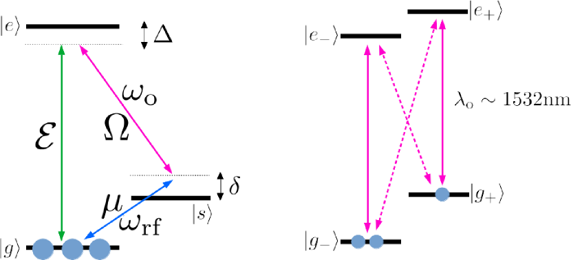
Figure 1: Left: Ideal $\Lambda$-scheme to implement resonant transduction. A low level spin transition, at few GHz between $\ket{g}$ and $\ket{s}$, is excited by the microwave field at $\omega_{\mathrm{rf}}$. The laser excites the $\ket{s}-\ket{e}$ transition in the optical domain at $\omega_{\mathrm{o}}$. This interaction are resonant or nearly resonant (detuned by few linewidths). The transduction signal (green arrow) is generated at $\omega_{\mathrm{o}}+\omega_{\mathrm{rf}}$. The field are characterized by their Rabi frequencies $\mu$, $\Omega$ and $\mathcal{E}$ for the optical Raman, microwave and transduction signal fields respectively. $\Delta$ and $\delta$ are the field detunings from the optical and spin transitions respectively. Right: Realistic level structure of Er³⁺:CaWO₄. The ground and optically excited states are actually spin Kramers doublets that split under magnetic field into $\ket{g_{-}}$,$\ket{g_{+}}$ and $\ket{e_{-}}$,$\ket{e_{+}}$ respectively. Additionally, in our temperature range ($\sim 2-3$K), the spins are only partially polarized so both $\ket{g_{-}}$ and $\ket{g_{+}}$ are populated. As a consequence, the transduction is possible on four transitions between the two doublets. This will be discussed in more details in 3.1.2 and 3.2.3

After having presented the experimental setup in 2, we will then characterize the cooperativities of the optical and spin transitions independently in 3.1. Finally, we present the results of the transduction process and its variation as a function of the accessible experimental parameters in 3.2. We continue with a detailed quantitative modeling of the transduction signal intensity in 4, and compare these theoretical results with the experiment. In the final section, we will discuss the discrepancy between the prediction and the experiment, and suggest some avenues for further studies in 5.

2 Experimental setup

2.1 Optical and RF excitations

We place the Er³⁺:CaWO₄ crystal ($5\times 4\times 3$ mm) in a rectangular RF copper resonator (dimensions $a\times b\times d=15\times 10\times 20$ mm parallel to our reference frame $\boldsymbol{x},\boldsymbol{y},\boldsymbol{z}$ respectively ) inside the inner bore of a superconducting coil providing the bias magnetic field $\boldsymbol{B_{0}}$ of typically 100 mT along $\boldsymbol{z}$ in our case (see Fig.2). The 4-mm dimension of the crystal along $\boldsymbol{y}$ correspond to the crystalline c-axis. The nominal concentration of erbium is 50 ppm. We excite the spins with a vector network analyzer (VNA) at $\sim$12 GHz (Anritsu MS46522B) through a single coaxial line and collect the reflexion $S_{11}$ coefficient. This allows to measure the RF cooperativity. The exact position of the crystal in the resonator and the intracavity field profile are detailed in B.

Following [38, eq.(6.40)], we expect the lowest resonant frequency to appear at $12.49$ GHz. In practice, we observe a narrow resonance near $12.29$ GHz with a quality factor of few thousands depending on the operating conditions (temperature, position of the crystal and length of the antenna). This resonance will be used for the spin excitation in the following. The length and position of the antenna (see Fig.2) are adjusted at room temperature to approach the critical coupling to the feed line so $S_{11}$ goes to zero in order to maximally excite the spins for a given input power.

The laser beam from a Velocity^® External Cavity Diode Laser around $1532$ nm enters and leaves the copper box through two holes (1mm diameter), crossing the crystal in a single-pass along its c-axis (4-mm dimension).

2.2 Transduction detection

The transduction signal should appear as a $\omega_{\mathrm{rf}}=2\pi\times 12.29$ GHz modulation of the transmitted laser beam at $\omega_{\mathrm{o}}$. This represents a relatively large frequency for optoelectronics devices so we decided to perform an heterodyne detection by generating a local oscillator (LO) $\omega_{\mathrm{lo}}=2\pi\times(12.29$ GHz$+44$ MHz) from the same laser using a standard lithium niobate electro-optic frequency modulator (EOM, see Fig.2). A low bandwidth photodiode ($<50$ MHz of a Thorlabs PDA255) can then record the beating between $\omega_{\mathrm{o}}+\omega_{\mathrm{rf}}$ and $\omega_{\mathrm{o}}+\omega_{\mathrm{lo}}$ at $44$ MHz in our case. The choice of this beatnote frequency is justified in appendix D.

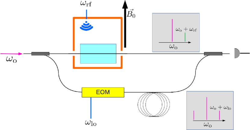
Figure 2: Transduction measurement setup. Half of the laser power, resonant with the optical transition passes through the crystal (single-pass along $\boldsymbol{y}$ parallel the crystalline c-axis) by a 1-mm diameter aperture in the cooper box (upper arm). The crystal is placed in a rectangular copper resonator in the inner bore of a bias coil cooled down at cryogenic temperature ($\sim 2.5$ K). The RF excitation is provided by the pin of a SMA connector (antenna). $\boldsymbol{B_{0}}$ is the bias magnetic field along $\boldsymbol{z}$. The heterodyne detection beats at $\omega_{\mathrm{rf}}-\omega_{\mathrm{lo}}$ between the opto-RF signal (upper arm) and the local oscillator generated by a fibered EOM (lower arm). The transduction signal appears as a sideband at $\omega_{\mathrm{o}}+\omega_{\mathrm{rf}}$ (see upper insert) after passing through the crystal. This beats on the photodiode with the $\omega_{\mathrm{o}}+\omega_{\mathrm{lo}}$ component of the local oscillator generated by the EOM (see lower insert). We adjust the beam polarization after the crystal (before recombination with the LO) to maximize the interference contrast on the photodiode. Both frequencies $\omega_{\mathrm{rf}}$ and $\omega_{\mathrm{lo}}$ are delivered by a dual channel VNA.

2.3 Transduction efficiency calibration

2.3.1 Electro-optics efficiency

Before considering the quantum perspectives of the transducer, we propose to use a classical metric to evaluate the opto-RF conversion efficiency. We here define the electro-optics efficiency as the normalized intensity of the sideband shifted by $\omega_{\mathrm{rf}}$ with respect to the carrier (relative intensity). This is a simple classical characterization of the transduction process that is directly related to experimentally measurable parameters.

The raw amplitude of the beatnote at $\omega_{\mathrm{rf}}-\omega_{\mathrm{lo}}$ depends on the relative laser power between the LO and the crystal transducer arms that form a Mach-Zender interferometer after recombination in Fig.2. On the LO side, the fibered EOM efficiency written $\eta_{\mathrm{lo}}$ (as the normalized intensity of the $\omega_{\mathrm{lo}}$ sideband) scales the amplitude of the recorded beatnote at $\omega_{\mathrm{rf}}-\omega_{\mathrm{lo}}$. We then measure $\eta_{\mathrm{lo}}$ independently by comparing the amplitude at $\omega_{\mathrm{lo}}$ with respect to the carrier through a commercial Fabry-Perot interferometer. At our working frequency $\sim$12 GHz, the fibered EOM efficiency is only $\eta_{\mathrm{lo}}\sim 7$% at 18.4 dBm input power (maximum power delivered by the VNA) because we exceed the nominal modulation bandwidth of the EOM and have a limited input driving power. Still, this is sufficient to observe and characterize the transduction signal.

Finally, there is no need to measure the power on both arms of the Mach-Zender interferometer because the transduction signal is a weak modulation of the carrier. Instead, we simply observe the Mach-Zender interferometer output DC signal on the photodiode. This fluctuates because the phase of the few meters long interferometer is not stable in time. There is no need to stabilize it for an AC measurement anyway. We record the amplitude of these slow temporal fluctuations between a maximum and a minimum as the voltage $V_{\mathrm{fringes}}$ that actually reveals the beating contrast (typically 80% in our case). This latter may be imperfect because of a small polarization mismatch, the spatial mode overlap being ensured by the single mode fiber recombiner. At the end, if the beatnote amplitude voltage recorded by the spectrum analyzer is $V_{\mathrm{sa}}$ then the electro-optics transduction efficiency $\eta_{\mathrm{eo}}$ is

$$\eta_{\mathrm{eo}}=\frac{1}{\eta_{\mathrm{lo}}}\left(\frac{V_{\mathrm{sa}}}{V_{\mathrm{fringes}}}\right)^{2}$$ (1)

This formula actually compares the measured power in the transduction sideband $\displaystyle\left(V_{\mathrm{sa}}\right)^{2}$ and the one in the local oscillator sideband $\displaystyle\eta_{\mathrm{lo}}\left(V_{\mathrm{fringes}}\right)^{2}$ that actually interfere to produce the beating signal as recorded independently.

We will use the electro-optics efficiency $\eta_{\mathrm{eo}}$ (expressed in dB typically) as a metric to analyze the experimental results. Nevertheless, it is important to carefully define the quantum number efficiency in the recent stimulating context.

2.3.2 Quantum number efficiency

By definition, the quantum number efficiency is the main metric for the quantum conversion process. As opposed to the electro-optics efficiency, we do not compare the intensity of the sideband at $\omega_{\mathrm{rf}}$ with respect to the optical carrier. Instead we here compare the photon number flux in the optical sideband at $\omega_{\mathrm{o}}+\omega_{\mathrm{rf}}$ and the RF photon flux. The powers are then $\eta_{\mathrm{eo}}P_{\mathrm{o}}$ for the optical sideband and $P_{\mathrm{rf}}$ for the RF respectively, where $P_{\mathrm{o}}$ is the laser power in the crystal and $P_{\mathrm{rf}}$ the RF power at the resonator input. So the quantum efficiency $\eta_{\mathrm{Q}}$ reads as

$$\eta_{\mathrm{Q}}=\frac{\left(\eta_{\mathrm{eo}}P_{\mathrm{o}}\right)/\omega_{\mathrm{o}}}{P_{\mathrm{rf}}/\omega_{\mathrm{rf}}}=\eta_{\mathrm{eo}}\frac{P_{\mathrm{o}}\omega_{\mathrm{rf}}}{P_{\mathrm{rf}}\omega_{\mathrm{o}}}$$ (2)

(1) and (2) connect the two definitions of the efficiencies.

The powers $P_{\mathrm{o}}$ and $P_{\mathrm{rf}}$ are experimental parameters. They are usually taken at the device inputs to focus on the conversion process and compensate for parasitic losses than can be avoided by technical improvements. Anticipating the description in 3.2.1, at the maximum RF source power, we have $P_{\mathrm{rf}}=37$ mW. The laser power inside the cryostat (corrected from losses though cryostat windows and crystal interfaces) is $P_{\mathrm{o}}=1.1$ mW. The power ratio (maximum RF) is then $\displaystyle\frac{P_{\mathrm{o}}}{P_{\mathrm{rf}}}=2.8\times 10^{-2}$ or -15.5 dB in log scale. Even if the powers have different orders of magnitude, we haven’t observed any saturation of both transitions confirming that the efficiencies are constant and well-defined in our range of parameters.

The frequency ratio is fixed by the level structure, in our case we have $\displaystyle\frac{\omega_{\mathrm{rf}}}{\omega_{\mathrm{o}}}=6.3\times 10^{-5}$ or -42.0 dB in log scale.

In typical experimental conditions (maximum power), we have $\eta_{\mathrm{Q}}=\eta_{\mathrm{eo}}-57.5$ dB when expressed in log scale. In conclusion, the efficiencies are proportional, they both characterize the transduction process that will be detailed in the next section.

3 Transduction

As discussed in the introduction, the RF and optical cooperativities are the key parameters to evaluate the transduction efficiency. They will be first characterized.

The reference method to measure the spin cooperativity consists in monitoring the $S_{11}$ from the VNA as the transition is tuned on resonance by sweeping the magnetic field. The shift induced by the spin scales as the RF cooperativity as we will show in 3.1.1.

Concerning the optical cooperativity, since we employ a non-resonant setup, the single-pass optical transmission can be directly recorded by a photodiode. As shown in 3.1.2, the cooperativity, equal to the optical depth in free space, can be deduced from the absorption spectrum.

We will then present the results of the transduction experiment in 3.2.

3.1 Cooperativities

3.1.1 RF cooperativity

The RF cooperativity can be deduced from the $S_{11}$ spectra for a varying magnetic field when the spin resonance is swept across as shown in Fig. 3.

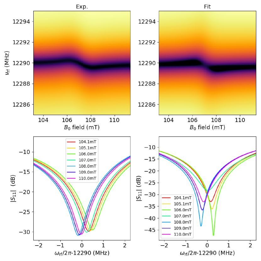
Figure 3: Absolute value of the $S_{11}$ coefficient. Top: Map (log. scale) of $|S_{11}|$ as a function of RF frequency (Y-axis) for a varying magnetic field (X-axis). Bottom: $|S_{11}|$ spectra for different characteristic values of the magnetic field. The experimental results are on the left and corresponding fit on the right (see the text for details). We observe a cavity resonance shift when the spin resonance is swept across.

The cavity response is described by the well-established input-output theory [39, 40] [41, Eq.(3.50)]

$$S_{11}(\omega_{\mathrm{rf}})=1-\frac{i\kappa_{c}}{\omega_{\mathrm{rf}}-\omega_{c}+i\frac{\kappa_{t}}{2}-W(\omega_{\mathrm{rf}})}$$ (3)

where $\kappa_{c}$ is the cavity coupling rate and $\kappa_{t}$ the damping rate ($\omega_{c}$ is the cavity resonant frequency). The spin interaction is contained in $W(\omega_{\mathrm{rf}})$ [41, Eq.(3.53)]

$$W(\omega_{\mathrm{rf}})=C_{\mu}\frac{i\kappa_{t}/2}{2i\frac{\omega_{\mathrm{rf}}-\omega_{s}}{\gamma}-1}$$ (4)

where $C_{\mu}$ is RF cooperativity [40], $\gamma$ the spin linewidth (FWHM) and $\omega_{s}$ the spin resonant frequency that varies with the magnetic field $B_{0}$ as $\omega_{s}=g\mu_{B}B_{0}/\hbar$ ($g$ is the erbium g-factor along $\boldsymbol{B_{0}}$ and $\mu_{B}$ the Bohr magneton).

We fit the map of $|S_{11}|$ in Fig. 3 to the model (3) & (4). So we obtain the different parameters: $\kappa_{t}=2\pi\times 8.57$ MHz corresponding to a quality factor of 1430, $\kappa_{c}=2\pi\times 4.52$ MHz demonstrating a close to critical coupling condition with $\kappa_{t}\approx 2\kappa_{c}$. The spin linewidth is measured to be $\gamma=2\pi\times 219.14$ MHz limited by the magnetic field inhomogeneity along the crystal dimensions. The fit predicts lower values for $|S_{11}|$ reaching -45 dB as compared to the minimum -30 dB that we observe. An ad-hoc introduction of extra losses (typically -15 dB) would certainly improve the fit accuracy, but this is difficult to justify a priori. So we stick to the original model and still expect a correct prediction of the parameters since these extra losses are almost invisible in the linear scale that we choose for the fitting procedure.

In any case, this leads to a RF cooperativity of $C_{\mu}=0.14$ in correct agreement with spin concentration and sample size (see C for details). This also gives an erbium g-factor of $g=8.20$ in good agreement with the reported values using this field orientation for $g_{\perp}$ [42, 33]. For comparison with magnetic field sweep, the spin linewidth $\gamma$ corresponds to $1.9$ mT or 1.7% bias field inhomogeneity.

We additionally extract a total attenuation coefficient of $-5.4$ dB mostly attributed to the coaxial line inside the cryostat.

The parameters obtained from this measurement allows to accurately characterize the excitation of spins coupled to the RF cavity.

3.1.2 Optical absorption

An equivalent analysis is conducted in the optical domain by finely sweeping our Velocity^® External Cavity Diode Laser around $\lambda_{\mathrm{o}}=1532.636$ nm (absorption line position at zero magnetic field) and monitor the crystal transmission with a photodiode in Fig.4. The polarization is along $\boldsymbol{z}$ (bias magnetic field) and is perpendicular to the crystalline c-axis.

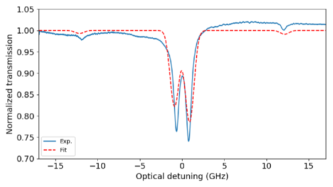
Figure 4: Absorption spectrum under a 105mT magnetic field (solid line). Four lines can be observed corresponding to level structure presented in Fig.1 (right). The optical wavelength is finely swept around the central value $\lambda_{\mathrm{o}}=1532.636$nm. The strongest lines correspond to the direct transitions $\ket{g_{-}}\rightarrow\ket{e_{-}}$, $\ket{g_{+}}\rightarrow\ket{e_{+}}$ (solid lines in Fig.1, right). The weakest to the crossed transitions $\ket{g_{-}}\rightarrow\ket{e_{+}}$, $\ket{g_{+}}\rightarrow\ket{e_{-}}$ (dashed lines in Fig.1, right). We fit data (dashed line) to extract the optical depth of the transitions (see text for details).

We observe four lines corresponding to the so-called direct and crossed transitions in Fig.1 (right). The two central lines are the direct ones (less than 1GHz detuning) and the crossed ones are positioned at roughly $\pm 12$ GHz. The former are stronger that the latter, without generality because this depends on the magnetic field orientation. The imbalance between the direct transitions, namely $\ket{g_{-}}\rightarrow\ket{e_{-}}$ and $\ket{g_{+}}\rightarrow\ket{e_{+}}$, is due to the finite temperature that partially polarize the spins into the $\ket{g_{-}}$ state. This is also present but much less visible on the crossed ones because of their weakness. So we model the transmission as the sum of four gaussian profiles and attribute two different absorption coefficients to the direct and crossed transitions. We also include the finite temperature to account for the Boltzmann thermal populations. We fit data and obtain the different parameters. The fit is visibly imperfect because of the numbers of parameters characterizing the transitions that must be completed by auxiliary parameters to describe the distorted absorption baseline. The latter is not flat because of the cryostat transmission path going through many insulating uncoated windows (vacuum ports, radiation shields and cold windows). We nevertheless keep the fitted parameters after convergence which give a realistic order of magnitude that can feed the model later on. We obtain an optical depth of $0.44$ and $0.016$ for the direct and crossed transitions respectively along the 4mm propagation direction of the crystal. The optical depths are normalized to a total population of one, so the finite temperature measurements exhibit a smaller absorption because the population is shared between $\ket{g_{-}}$ and $\ket{g_{+}}$. In other words, for an expected fully polarized spins ensemble, the direct and crossed transitions from $\ket{g_{-}}$ would have an optical depth of $0.44$ and $0.016$ respectively.

The fitted optical linewdith is $\Gamma=2\pi\times 1750$ MHz (FWHM), a typical value for low concentration rare-earth samples. The value is compatible but still larger than the previously reported inhomogeneous linewidth in Er³⁺:CaWO₄, even if the exact lineshape and measurement conditions cannot be compared at this level [43].

This concludes the characterization of the spin and optical transitions independently in terms of cooperativity. The parameters extracted from both fits will be used to model the transduction efficiency in 4. The corresponding experimental results will be detailed now.

3.2 Transduction characterization

Using the detection setup sketched in Fig.2 and described in 2, the opto-RF transduction signal appears as a $44$ MHz beating between the spin signal frequency $\omega_{\mathrm{o}}+\omega_{\mathrm{rf}}$ and the local oscillator $\omega_{\mathrm{o}}+\omega_{\mathrm{lo}}$. The photodiode is directly connected to a spectrum analyzer (Agilent E4402B, centered at 44 MHz, 50 kHz span, 1 kHz resolution). The amplitude of the beatnote peaks (raw data) varies from -75 dBm (maximum signal) to -95 dBm (noise floor) corresponding to the measured voltage $V_{\mathrm{sa}}$ as defined in 2.3. The data will be displayed in terms of electro-optics efficiency $\eta_{\mathrm{eo}}$ (in dB, left plot axis) using (1) and quantum number efficiency efficiency (in dB, right plot axis) since both are simply related by (2).

We will first characterize the transduction signal as a function of the magnetic field (spin detuning) in 3.2.1 and $\omega_{\mathrm{rf}}$ (cavity detuning) in 3.2.2 for a given laser wavelength of $\lambda_{\mathrm{o}}=1532.727$ nm corresponding to the $\ket{g_{+}}\rightarrow\ket{e_{-}}$ transition. We will finally vary the optical wavelength in 3.2.3 to compare the different absorption lines.

3.2.1 Spin detuning

We keep the RF and laser frequencies constant as $\omega_{\mathrm{rf}}=2\pi\times 12.29$ GHz and $\lambda_{\mathrm{o}}=1532.727$ nm and we sweep the magnetic field to tune the spins on resonance (see Fig. 5).

The input RF power is 18.4 dBm, the maximum power of our VNA as directly measured at low frequency ($\sim$1 GHz). The RF power at the cavity input can be inferred from the -5.4 dB coaxial line attenuation (extracted for the fit described in 3.1.1) so we assume the input RF power to be reduced by -2.7 dB at the cavity level namely $P_{\mathrm{rf}}=37$ mW or 15.7 dBm.

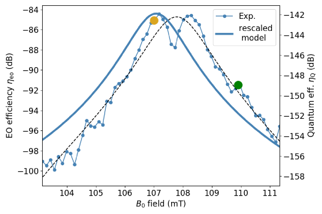
Figure 5: Transduction efficiency as a function of the spin detuning. The latter is adjusted by scanning the magnetic field across the resonance as in Fig.3. The colored circles correspond to the values $B_{0}=107.0$ mT and $109.9$ mT that will be used for a RF frequency scanning in Fig.6. The left axis represents the electro-optics efficiency and the right one the quantum efficiency. Both are related by (2). The solid line is the theoretical prediction affected by a rescaling factor as will be discussed in 4.2

The electro-optics efficiency is globally weak with a maximum of -84 dB approximately, using (1) to convert the measured beatnote into a transduction performance. Our noise detection floor is -105 dB when expressed in electro-optics efficiency. A quantitative analysis will be developed in 4.

Concerning the linewidth of the beatnote, we essentially retrieve the spin linewidth $\gamma$ as measured in 3.1.1. For the experimental curve, the presence of dip at center and the slight shift from the spin resonance is not reliable from shot to shot. This is attributed to instability of the magnetic field during and between the sweeps of the magnet (hysteresis). Apart from the linewidth, that is well predicted, the model is down scaled by -11 dB to retrieve the experimental maximum as will be discussed in 5.

3.2.2 Cavity detuning

Under the same experimental conditions ($\lambda_{\mathrm{o}}=1532.727$ nm and 18.4 dBm RF power), we now vary the RF frequency for two values of the magnetic field ($B_{0}=107$ mT and $109.9$ mT) as plotted in Fig.6.

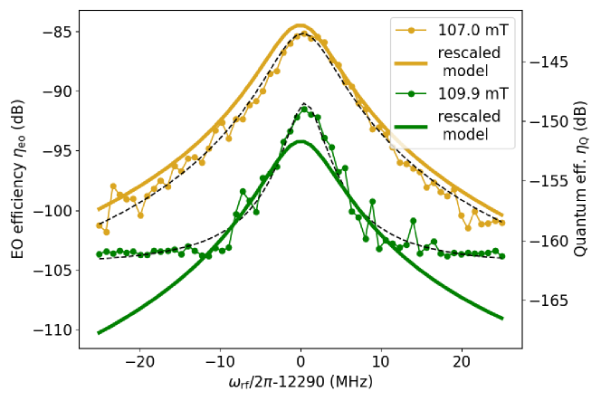
Figure 6: Transduction efficiency as a function of the cavity detuning. We vary the $\omega_{\mathrm{rf}}$ around the cavity resonance at $12.290$ GHz spanning $50$ MHz. $B_{0}=107$ mT and $109.9$ mT correspond respectively to spins on resonance or slightly detuned from the cavity (see Fig. 5). The dashed lines are a lorentzian fit to the data. The left axis represents $\eta_{\mathrm{eo}}$ and the right one $\eta_{\mathrm{Q}}$. The dashed line is a lorentzian fit to the data. The solid lines are the expectation from the model detailed in 4.2

One roughly retrieves the cavity linewidth on the electro-optics efficiency. The curves are well approximated by a lorentzian fit (dashed lines in Fig.6) with 8 MHz and 4.3 MHz linewidths for $B_{0}=107$ mT and $109.9$ mT respectively. The first value (8 MHz at $B_{0}=107$ mT) should be compared to the $\kappa_{t}=2\pi\times 8.57$ MHz cavity linewidth obtained from Fig.3. The second value (4.3 MHz at $109.9$ mT) is narrower than $\kappa_{t}$ but is visibly limited by our noise detection floor of -105 dB which limit the experimental peak amplitude and in turn gives an artificially low linewidth. A quantitative comparison of the efficiency will be detailed in 5.

3.2.3 Wavelength dependency

Keeping the spin RF excitation at the previously described optimal conditions, we now vary the laser excitation wavelength. The laser is finely tuned step by step ($\sim 0.3$ GHz steps). After each step, we record the laser wavelength (Burleigh WA-1000 Wavelength Meter) and acquire the transduction signal in Fig.7 as detailed in 2.3.

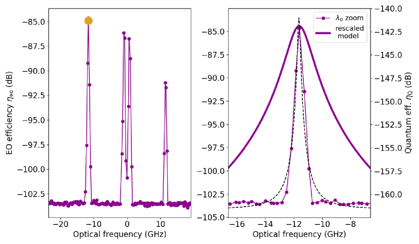
Figure 7: Transduction efficiency as a function of the optical wavelength for $B_{0}=107.0$ mT. Left: broad spectrum covering the different absorption lines observed in Fig.4. The coloured circle correspond to a wavelength of $\lambda_{\mathrm{o}}=1532.727$ nm at which other measurements have been performed. Right: Narrow scan around $\lambda_{\mathrm{o}}$ compared to the prediction of the model (solid line) that will be presented in 4.2. The dashed is a lorentzian fit to the data (linewidth 191 MHz). As before, the left axis represents $\eta_{\mathrm{eo}}$ and the right one $\eta_{\mathrm{Q}}$ as in Figs.5 and 6.

The transduction spectrum in Fig.7 should be compared to the optical absorption in Fig.4. One retrieve the position of the different absorption lines corresponding to the level structure of Fig.1 (right). The efficiency tends to decrease from one peak to the other when the optical frequency increases. The tendency is not reproducible from one data set to the other and may be explained by the narrowness of the lines compared to the frequency steps of $\sim 0.3$ GHz steps which makes the measurement quite sensitive to the experimental instabilities.

In any case, the transduction efficiency does not follow the strength of the transitions. The weakest and the strongest transitions in Fig.4 roughly give the same transduction signal. This is actually not surprising because the appearance of the transduction signal in a $\Lambda$-system connects the strength of both optical transitions involved in the non-linear process (namely $\ket{s}-\ket{e}$ and $\ket{g}-\ket{e}$, Fig.1, left), more precisely the product of the direct and the crossed transitions strengths. The latter is generally constant within $\Lambda$-systems formed by Kramers doublets in the ground and excited states. This qualitative explanation will be discussed in the light of the theoretical model developed in the next section 4.

Finally, in Fig.7 (right), we zoom on one peaks and compare the measurement to the model. This latter predicts a transduction optical linewidth of $\Gamma=2\pi\times 1750$ MHz equals to the optical absorption linewidth as in Fig.4. The transduction linewidth is narrower by an order of magnitude (191 MHz FWHM). This is a unexpected feature that will discussed in 5.

4 Theoretical modeling

The transduction process in a $\Lambda$-scheme as sketched in Fig.1 can be described by Schrödinger-Maxwell model that we detail in A. We present the result in the form of a input-output solution.

4.1 Input-output solution

The outgoing signal field after propagation through the crystal (length $z$) reads as an integral solution for $\mathcal{E}(z)$ after a propagation $z$ (36):

$$\mathcal{E}(z)=\frac{1}{2\delta}\left[\exp\left(\frac{-2i\delta\Gamma}{4\delta\Delta-\Omega^{2}}\alpha_{\mathcal{E}}\,z\right)-1\right]\Omega\times\mu$$ (5)

The different parameters are schematically represented in Fig.1(left). The input-output solution (5) relates the different fields represented by their Rabi frequencies: $\mu$ for RF field, $\Omega$ for the optical Raman field and $\mathcal{E}$ for the transduction signal. The experimental parameters $\Gamma$ and $\gamma$ are the optical and spin linewidths (FWHM) respectively. $\Delta$ and $\delta$ are the detunings of optical and spin transitions respectively. $\alpha_{\mathcal{E}}$ is the absorption coefficient on the $\ket{g}-\ket{e}$ transition, or in other words, $\alpha_{\mathcal{E}}\,z$ is the optical cooperativity.

In order to define the electro-optics efficiency, one has to compare the intensity of the optical field $\Omega$ and the generated transduction signal $\mathcal{E}$ at the output of the medium. We choose to express the fields in units of Rabi frequencies which is a natural choice to write the light-matter interaction Hamiltonian (29). Nevertheless, the comparison of the different fields intensities is then indirect and requires the introduction of the transition dipole moments. This will be discussed specifically in 4.2. One may be also surprised by the predominance of the optical cooperativity on the $\ket{g}-\ket{e}$ transition $\alpha_{\mathcal{E}}\,z$, because one expects a symmetric dependency with respect to the fields involved in the non-linear mixing process $\mu$ , $\Omega$ and $\mathcal{E}$. This contradiction is only apparent because of the choice of units as will made explicit in defining the electro-optics and quantum efficiencies in 4.2 and 4.3.

In the meantime, one can already discuss and simplify the expression (5). The right-hand side term $\Omega\times\mu$ represent the lowest order frequency mixing process that generate the transduction signal from the optical and RF fields. Strictly speaking, the transduction can be seen as a sum-frequency generation, namely a second order nonlinear optical-RF process as already noted [10]. The prefactor $\displaystyle\frac{2\delta\Gamma}{4\delta\Delta-\Omega^{2}}$ potentially introduces high-order contributions from $\Omega^{2}$, $\Omega^{4}$ … if written as a Taylor expansion so this is not a second order nonlinear process anymore. It should be nevertheless noted that the intensity $\Omega^{2}$ is in practice smaller than $\delta\Delta$. $\Delta$ is indeed of the order of the optical inhomogeneous linewidth, experimentally much larger than $\Omega$ [44, 45]. This further simplify the analysis.

Additionally, one can consider the low absorption limit $\alpha_{\mathcal{E}}\,z\ll 1$, keeping only the first order term in the expansion of $\left[1-\exp\left(\cdots\alpha_{\mathcal{E}}\,z\right)\right]$

$$\mathcal{E}(z)=\left[\frac{-i\Gamma}{4\delta\Delta}\alpha_{\mathcal{E}}\,z\right]\Omega\times\mu$$ (6)

This simplified expression will be used for the rest of the paper, and can be used to write the electro-optics and quantum efficiencies in 4.2 and 4.3.

4.2 Electro-optics efficiency

4.2.1 Definition

As previously discussed, we compare the intensity of the input optical field $\Omega$ and the generated signal $\mathcal{E}$ to define electro-optics efficiency. The Rabi frequencies $\Omega$ and $\mathcal{E}$ are related to the electric field amplitudes $E_{\Omega}$ and $E_{\mathcal{E}}$ by $\Omega=\displaystyle\frac{\mathcal{P}_{\Omega}E_{\Omega}}{\hbar}$ and $\mathcal{E}=\displaystyle\frac{\mathcal{P}_{\mathcal{E}}E_{\mathcal{E}}}{\hbar}$ respectively where $\mathcal{P}_{\Omega}$ and $\mathcal{P}_{\mathcal{E}}$ are the transition dipoles of the optical transitions for the Raman and signal fields respectively.

The electro-optics efficiency is then $\eta_{\mathrm{eo}}=\displaystyle\frac{\left|E_{\mathcal{E}}\right|^{2}}{\left|E_{\Omega}\right|^{2}}$. This can be obtained directly from (6) by introducing the ratio of the transitions dipole moments (sometimes called the branching ratio) or equivalently $\displaystyle\sqrt{\frac{\alpha_{\mathcal{E}}}{\alpha_{\Omega}}}$ introducing the absorption coefficients of both transitions, leading to

$$\eta_{\mathrm{eo}}=\left|\frac{\Gamma}{4\delta\Delta}\right|^{2}\alpha_{\mathcal{E}}z\times\alpha_{\Omega}z\times\left|\mu\right|^{2}$$ (7)

The formula involves spectroscopic parameters (absorption coefficients and linewidths) deduced from the experimental measurements on one side (see 3.1.1 and 3.1.2) and the Rabi frequency of RF field $\mu$ on the other side. The expression is more symmetric since it involves equally the cooperativities $\alpha_{\mathcal{E}}z$ and $\alpha_{\Omega}z$ on the both optical transitions.

When defining the electro-optics efficiency, essentially comparing $\Omega$ and $\mathcal{E}$, without surprise, the RF power $\left|\mu\right|^{2}$ appears as a parameter.

In practice, the relative strengths of the optical transitions need to be deduced from absorption measurements because the optical electric-dipole excitation is forbidden to the first order relying on the so-called forced electric-dipole and/or allowed magnetic-dipole (as for erbium) transitions [45].

(7) involve the product $\alpha_{\mathcal{E}}\times\alpha_{\Omega}$ so the transduction efficiency do not depend on which transition is pumped with $\Omega$ (direct or crossed in Fig.1). In other words, if a weak transition is pumped with $\Omega$ then a strong transition will generate $\mathcal{E}$ or the other way around, then the resulting efficiency will be the same for both cases since the product of strengths will be involved. That is the reason why in Fig.7 the efficiency does not follow the relative strength of the excited transitions.

The RF Rabi frequency $\mu$ can be directly deduced a priori from the g-factors (magnetic dipole of the spin) and the value of the AC magnetic field inside the resonator (intracavity RF power). In other words, the spin transition is magnetic-dipole allowed to pursue the analogy, so $\left|\mu\right|^{2}$ can be deduced from the RF cavity parameters and the input power (directly proportional). The well-known calculation of the AC magnetic field distribution in a rectangular resonator is reminded in B.

The RF Rabi frequency follows the resonance of the cavity given by the relection coefficient (3). As detailed in B, we finally obtain (44) in the low spin cooperativity limit:

$$\mu=\frac{4g_{x}}{\hbar}\sqrt{\mu_{0}}\frac{a}{\sqrt{d^{2}+a^{2}}}\sqrt{\frac{P_{\mathrm{rf}}}{V}}\sqrt{\frac{2\kappa_{c}}{4\left(\omega_{\mathrm{rf}}-\omega_{c}\right)^{2}+\kappa_{t}^{2}}}$$ (8)

where $g_{x}=g_{\perp}$ is $g$-factor along the $x$ direction of the RF field. $a$, $d$ and $V$ are the resonator dimensions and volume, $P_{\mathrm{rf}}$ is the input resonator power, as defined in B.

4.2.2 Finite temperature and population distribution

Moving away from the ideal structure discussed in Fig.1 (left), namely all the atomic population is in the level $\ket{g}$ (zero temperature), it is important to consider the imperfect polarization of the spin states as in our case at a temperature of few kelvins. The population is distributed between $\ket{g}$ and $\ket{s}$, written $\rho_{\mathrm{gg}}$ and $\rho_{\mathrm{ss}}$ respectively. There is no population in the excited state because of the huge energy gap.

Rigorously accounting for the atomic population requires the use of the density matrix formulation, we won’t detail this calculation here, as it’s lengthy, can be found in a number of textbooks [46, 47] and ultimately gives an intuitive result. The imperfect polarization can be introduced by by-hand in the simplified formula (6). The population difference $\rho_{\mathrm{gg}}-\rho_{\mathrm{ss}}$ actually scales the RF spin coupling term, or in other words, for a perfect population balance there is no interaction with the spin. This annihilation would correspond to a perfect balance between the absorption and stimulated emission on the $\ket{g}-\ket{s}$ transition. Starting for the structure in Fig.1 (left), one could alternatively consider the reverse situation with $\ket{s}$ fully populated and show that both schemes would interfere destructively leading to the annihilation of the opto-RF process when both levels are populated. This interpretation can be formally justified using the density matrix, but for the present analysis, we can stay at the intuitive level and rescale $\mu\rightarrow\left(\rho_{\mathrm{gg}}-\rho_{\mathrm{ss}}\right)\mu$. This readily affects the efficiency as

$$\eta_{\mathrm{eo}}=\left|\frac{\Gamma}{4\delta\Delta}\right|^{2}\alpha_{\mathcal{E}}z\times\alpha_{\Omega}z\times\left|\mu\right|^{2}\left(\rho_{\mathrm{gg}}-\rho_{\mathrm{ss}}\right)^{2}$$ (9)

Beyond the rescaling of the efficiency, the absorption terms $\alpha_{\mathcal{E}}$ and $\alpha_{\Omega}$ should be handled with precaution: $\alpha_{\mathcal{E}}$ ($\alpha_{\Omega}$ resp.) is the absorption coefficient on the $\ket{g}-\ket{e}$ transition ($\ket{g}-\ket{s}$ resp.) if $\ket{g}$ is fully populated ($\ket{s}$ resp.).

The absorption spectrum as in Fig.4 actually measures $\alpha_{\mathcal{E}}$ and $\alpha_{\Omega}$ and already accounts for the current population at a given temperature in the states $\ket{g}$ and $\ket{s}$ by assuming a thermal population proportional to $\rho_{\mathrm{gg}}=\displaystyle\frac{1}{1+\exp\left(-\hbar\omega_{s}/kT\right)}$ and $\rho_{\mathrm{ss}}=\displaystyle\frac{\exp\left(-\hbar\omega_{s}/kT\right)}{1+\exp\left(-\hbar\omega_{s}/kT\right)}$. From the optical spectrum fit, the population imbalance is inferred to $\displaystyle\left(\rho_{\mathrm{gg}}-\rho_{\mathrm{ss}}\right)=0.12$ that can feed (9).

In conclusion, the electro-optics efficiency (9) which includes the RF Rabi frequency (8) only contains already measured parameters that can be used to compare the experimental results with the previously derived model as we will discuss in 4.4.

4.3 Quantum number efficiency

4.3.1 Definition

As compared to the electro-optics efficiency defined in 4.2, it is important to properly describe the quantum efficiency. The latter is the main figure of merit for a quantum transducer. Again, (6) characterizes the mixing process of the optical pump $\Omega$ with the RF field $\mu$ (and vice-versa) to generate the optical signal $\mathcal{E}$. As previously explained, the electro-optics efficiency essentially compares the intensities of the signal $\mathcal{E}$ and the pump $\Omega$. The quantum efficiency compares different quantities, namely the number of photons in the optical signal $\mathcal{E}$ and the RF field $\mu$. From this point of view, the optical pump $\Omega$ is just a classical parameter.

The Rabi frequencies of the optical field $\mathcal{E}$ and the RF $\mu$ are related to the quantized fields, called $\mathcal{A}$ and $\mathcal{B}$ in the following, by the coupling constant $g_{\mathcal{E}}$ and $g_{\mu}$ respectively in the sense of the Jaynes–Cummings model. So we have $\displaystyle\mathcal{E}=g_{\mathcal{E}}\,\mathcal{A}$ and $\displaystyle\mu=g_{\mu}\,\mathcal{B}$ respectively.

In (6), the term $\displaystyle\frac{\Gamma}{4\delta\Delta}\Omega$ can be taken as a parameter, but it should also be noted that $\alpha_{\mathcal{E}}$ also contains a contribution from the coupling rate $g_{\mathcal{E}}$ between light and atoms. Both are related by the following standard expressions, for the coupling constant

$$g_{\mathcal{E}}=d_{\mathcal{E}}\sqrt{\frac{\omega_{o}}{2\hbar\epsilon_{0}V_{\mathcal{E}}}}$$ (10)

where $d_{\mathcal{E}}$ is the transition dipole and $V_{\mathcal{E}}$ the quantization volume whose choice will be discussed extensively in 4.3.2, and for the absorption coefficient

$$\alpha_{\mathcal{E}}=\frac{\mathcal{N}\omega_{o}{d_{\mathcal{E}}}^{2}}{\hbar c\epsilon_{0}\Gamma}$$ (11)

where $\mathcal{N}$ is the atomic density. So $\alpha_{\mathcal{E}}$ can be alternatively expressed as a function of $g_{\mathcal{E}}$ with (10)

$$\alpha_{\mathcal{E}}=\frac{2\mathcal{N}V_{\mathcal{E}}{g_{\mathcal{E}}}^{2}}{c\Gamma}$$ (12)

This allows to express (6) in terms of quantized fields $\mathcal{A}$ and $\mathcal{B}$ as

$$\mathcal{A}=\left[\frac{-i\Omega}{4\delta\Delta}\right]\,\frac{2\mathcal{N}V_{\mathcal{E}}z}{c}\,g_{\mathcal{E}}g_{\mu}\cdot\mathcal{B}$$ (13)

Since the optical and RF fields play an equivalent role, the expression can be made more symmetric by introducing the cooperativities that we used as key parameters to characterize the experimental data. In cavity quantum electrodynamics (cavity QED), the spin cooperativity is defined as

$$C_{\mu}=\frac{g_{\mu}^{2}N_{\mu}}{\gamma\kappa_{c}}$$ (14)

where $N_{\mu}=\mathcal{N}V_{\mathrm{crystal}}$ is the number of excited spins ($V_{\mathrm{crystal}}$ is the crystal volume) [40]. Usual cavity QED expressions can be used without ambiguity for the RF spin coupling, but this is not the case for the optical excitation because there is no optical resonator in our approach. The quantization of the optical field in free-space and the definition of the corresponding cooperativity should then be handled with precaution as we will see now.

4.3.2 Choice of quantization volume

Our experimental choice, namely a resonant RF cavity but free-space optical pass, may be a source of confusion when considering the quantum efficiency by comparing the number of photons. As we have seen, the efficiency definition introduces a quantization volume for the optical field that deserves a discussion. Indeed the quantization volume of the free-space optical pass should be adequately chosen to illustrate the transduction process. The transverse dimension of the optical photon are essentially imposed by the beam size (cross-section $S_{\mathcal{E}}$) but the spatial extension (pulse length) actually depends on the pulse duration. Surprisingly, the latter should depend on the RF pulse length. In other words, optical and RF photons should have the same duration. As a consequence, we impose for the optical cooperatitiy to read as

$$C_{\mathcal{E}}=\frac{g_{\mathcal{E}}^{2}N_{\mathcal{E}}}{\Gamma\kappa_{c}}$$ (15)

$N_{\mathcal{E}}=\mathcal{N}S_{\mathcal{E}}z$ is the number of atoms in the optical path (cross-section $S_{\mathcal{E}}$ and length $z$). That is to say, we impose the optical quantization volume to depend on the RF cavity linewidth as

$$V_{\mathcal{E}}=S_{\mathcal{E}}\frac{c}{2\kappa_{c}}$$ (16)

where $\displaystyle\frac{c}{2\kappa_{c}}$ is the photon spatial extension in free-space. This choice may appear arbitrary and surprising because $N_{\mathcal{E}}\neq\mathcal{N}V_{\mathcal{E}}$ for example. But this is driven by the physics of the conversion process and has the advantage to give consistent results at the end, somehow extending the cavity QED model to free-space approaches, that can be explored experimentally.

With this choice, one can alternatively express the optical cooperativity $C_{\mathcal{E}}$ defined by (15) using the absorption coefficient (11) and the coupling constant (10) as

$$C_{\mathcal{E}}=\alpha_{\mathcal{E}}z$$ (17)

Without surprise, cooperativity and optical depth are the same in free-space, as noted early in the context of quantum memories [48]. This result is quite intuitive, thus supporting our choice of quantization volume.

4.3.3 Expression as function of the cooperativities

(13) can now be simplified by introducing the cooperativities defined by (14) and (15).

$$\mathcal{A}=\left[\frac{-i\Omega\sqrt{\Gamma\gamma}}{4\delta\Delta}\right]\,\sqrt{\frac{S_{\mathcal{E}}z}{V_{\mathrm{crystal}}}}\sqrt{C_{\mathcal{E}}}\sqrt{C_{\mu}}\cdot\mathcal{B}$$ (18)

The quantum number efficiency $\eta_{\mathrm{Q}}$ compares the photon numbers in the quantized fields $\mathcal{A}$ and $\mathcal{B}$ leading to the expression

$$\eta_{\mathrm{Q}}=\left|\frac{\Omega\sqrt{\Gamma\gamma}}{4\delta\Delta}\right|^{2}\,{C_{\mathcal{E}}}{C_{\mu}}\,\frac{S_{\mathcal{E}}z}{V_{\mathrm{crystal}}}$$ (19)

(19) should be compared to its equivalent electro-optics efficiency expression (7). In a same manner, if we account for an incomplete polarization in the ground state, the efficiency is rescaled by the factor $\left(\rho_{\mathrm{gg}}-\rho_{\mathrm{ss}}\right)^{2}$ as in (9).

4.4 Discussion

(9) and (19) describe the same physical process with different points of view. The quantum efficiency (19) shows the symmetric role of the laser and RF fields cooperativities as opposed to (9) where the spin collective coupling is somehow hidden in the definition of the Rabi frequency. Our derivation of (19) leads to the same expression of the cavity QED approach, when both fields are enhanced in resonators [10]. In 4.3, we simply illustrate the experimental comparison between $\eta_{\mathrm{eo}}$ and $\eta_{\mathrm{Q}}$ than can be done directly with (2). Nevertheless, we have shown that the well-established Schrödinger-Maxwell description leads to the same expression that can be derived from the cavity QED formalism. This is important in our case since the optical field is propagating in free-space (single-pass). In any case, (19) shows the prevalence of the cooperativities and the intensity of the pump field $\Omega$ as key parameters that should drive the process understanding and the experimental design.

As discussed in 4.2, (9) allows to predict the efficiency by evaluating the experimental parameters. This is sufficient to compare the data with the model. Even if the expression (19) involves different parameters (that could be measured independently). it derives from the same expression. So for a given set, (9) and (19) are proportional and related by (2). In Figs. 5, 6 and 7, we use two efficiency axes, left and right, for (9) and (19) respectively. They simply differ by 57.5 dB.

The discrepancy between the experimental data and the model can now be discussed specifically.

5 Analysis

In Figs. 5, 6 and 7, the model only qualitatively reproduces the data. Indeed, to roughly reproduce the observed efficiencies, we systematically downscale the model by 11 dBm (in the three Figs. 5, 6 and 7). More precisely, the experimental efficiency $\eta_{\mathrm{eo}}$ peaks typically at -84 dBm in the optimal conditions (on-resonance fields) where the model predicts -73.4 dBm.

Concerning the RF excitation, we note that the linewidths, when we vary the spin detuning in Fig.5 or the cavity detuning in Fig.6, are properly reproduced when the measured signal largely exceed our noise level. Only the 11 dBm discrepancy remains.

Concerning the optical linewidth of the transduction signal in Fig.4, we find a FWHM of 191 MHz, that is much narrower than the absorption peaks $\Gamma=2\pi\times 1750$ MHz in Fig.7, by an order of magnitude. The observed value of 191 MHz is surprisingly close to the spin linewidth $\gamma=2\pi\times 219.14$ MHz measured in 3.1.1. This points to a possible correlation between the spin and optical transitions, the effect of which has still to be assessed. In any case, the global discrepancy cannot be simply explained within our framework and deserves further investigations.

The fact that we obtain a transduction feature narrower than the inhomogeneous absorption profile may also indicate that the mixing process actually resolves the inhomogeneous linewidth, comparable to the spectral hole burning mechanism, without reaching the homogeneous linewidth though ($<$MHz). This may partially explain the discrepancy with the model. Indeed, spectral hole burning and more generally optical pumping dynamics is not included in our model because we assume in A.1 that the population stays in the ground state (so-called perturbative regime), or at minimum that the population distribution is steady (see 4.2.2). This would require further theoretical modeling and would for sure introduce another level of non-linearity with the optical pumping intensity (noted $\Omega^{2}$) acting not only on the coherence as in (30) and (31), but also on the population as an optical pumping mechanism.

We conclude with a last remark to further explain the limitations of the theoretical model and the discrepancy with the experiment. We have briefly discussed the nature of optical transitions in 4.2 driven by $\Omega$ and $\mathcal{E}$, forced electric or magnetic dipole, both of which are possible in the case of erbium. In terms of absorption, there is no distinction. This is not the case for the transduction process. The branches of the $\Lambda$-system must in fact be of the same nature $\Omega$ and $\mathcal{E}$ without imposing any special constraint on the spin transition driven by $\mu$, as judiciously noted in [49, 23]. A fictitious pathological case, where one branch of the $\Lambda$-system would be purely magnetic dipole and the other purely electrical dipole, prohibits the non-linear mixing process. The interaction Hamiltonian introduced in the section A here assumes couplings of the same nature for the transitions, generally electric dipole for the sake simplicity, but an equivalent model would give the same result for a magnetic dipole coupling [50]. A measurement of absorption solely cannot determine the nature of the transitions, and can only roughly predict the efficiency of the transduction process. This uncertainty should be minimized in our case, since the magnetic field is perpendicular to the crystal c-axis, which should avoid a complete disjunction in the nature of the $\Lambda$-system transitions [51]. However, a rigorous evaluation can only be made through a detailed analysis of the crystal field and the nature of the wave functions in the levels involved [49].

6 Conclusion

We observed and carefully characterized the opto-RF transduction process in Er³⁺:CaWO₄ using the resonant excitations of the spin and optical transitions in a $\Lambda$-system. Our work can alternatively be seen as the quantitative extension of the Raman heterodyne detection technique, since we carefully model the intensity of the beating signal. We have decided to operate a simplified setup, employing a rectangular RF resonator to enhance the spin driving and a single-pass laser beam to excite the optical transition. This allows to extract the different experimental parameters independently that can feed our Schrödinger-Maxwell model.

We reach an electro-optics efficiency of -84 dB for 15.7 dBm RF power corresponding to a quantum efficiency of -142 dB for 0.4 dBm optical power. We carefully define both quantities that describe the same process from different points of view. The model convincingly predicts the different spin-related linewidths but fails to reproduce the optical linewidth and overestimates the efficiencies. We bring out a systematic discrepancy and downscale the model by 11 dBm to fit data. The origin of this discrepancy is not understood. In the context of quantum transduction, where efficiency matters, we hope our analysis will stimulate further studies, both theoretical and experimental, involving other materials.

To conclude, it is important to return to the main context motivating our study. How can we increase the quantum efficiency close to unity ? The question here is to gain orders of magnitude compared to our proof of principle, which is limited to -142 dB. The configuration we have chosen (optical single-pass) can be optimized by using Er³⁺:Y₂SiO₅ for example, whose bare cooperativity (absorption) remains better and the transitions narrower, with a direct impact on the efficiency (19). A higher optical power can then be used to achieve typically -90 dB [26]. Another order of magnitude can be achieved by fully polarizing the spins at reduced temperature (10-20 mK), which will in any case be necessary for the interconnection with superconducting qubits for example. There’s still a long way to reach a unit efficiency.

The use of an optical cavity then offers a typical gain of four orders of magnitude compared with single-pass configuration, as the cooperativity follows proportionally the finesse of the optical resonator [26]. Finally, the obvious way to perfect the job is to use fully concentrated materials [15]. Little studied in optics, they are particularly attractive compared with diluted samples (10-100 ppm), since the concentration and therefore the cooperativity increase by 4 or 5 orders of magnitude. At very low temperatures, they can even exhibit magnetic ordering, further narrowing the magnon resonances, whose sharpness increases the efficiency. Their study under coupled optical and RF excitations clearly opens up a new field for rare-earth doped crystals.

Appendix A Schrödinger-Maxwell model

The dynamics of three-level atoms under field excitation (optical or RF) can be found in many textbooks. The interest for the coherent excitation of $\Lambda$-scheme has been renewed by the observation of electromagnetically induced transparency opening a wide spectrum of quantum memory protocols [18]. This represents a solid background for the theoretical description of the opto-RF transduction process even if this connection has not been made explicit so far. A modal description as a generalization of cavity quantum electrodynamics with different fields is usually preferred without specific assumption on the physical system [11, 10]. We choose to stick to the Schrödinger equation for three-level atoms as depicted in Fig.8 even if both approaches are equivalent to some extend.

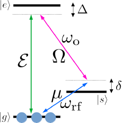
Figure 8: $\Lambda$-scheme to implement resonant transduction similar to Fig.1 with the notations for the model in 4. $\mu$ is the Rabi frequency of RF field on the spin transition $\ket{g}-\ket{s}$ (frequency $\omega_{\mathrm{rf}}$ detuned by $\delta$). $\Omega$ is the Rabi frequency of optical field on the transition $\ket{s}-\ket{e}$ (frequency $\omega_{\mathrm{o}}$ detuned by $\Delta$). The transduction signal is generated at $\omega_{\mathrm{o}}+\omega_{\mathrm{rf}}$ with a Rabi frequency $\mathcal{E}$ on the $\ket{g}-\ket{e}$ transition. We first assume that the level $\ket{g}$ is solely populated (zero temperature). This assumption will be correct by-hand to account for the presence of population in $\ket{s}$ as well (finite temperature in 4.2.2).

A.1 Schrödinger equation for three-level atoms in the perturbative regime

For three-level atoms, labeled $|g\rangle$, $|e\rangle$ and $|s\rangle$ for the ground, excited and spin states depicted in Fig.8, the rotating-wave probability amplitudes $C_{g}$, $C_{e}$ and $C_{s}$ respectively are governed by the time-dependent Schrödinger equation [52, eq. (13.29)]:

$$i\partial_{t}\left[\begin{array}[]{c}C_{g}\\ C_{e}\\ C_{s}\\ \end{array}\right]=\left[\begin{array}[]{ccc}0&\displaystyle\frac{\mathcal{E}^{*}}{2}&\displaystyle\frac{\mu^{*}}{2}\\ \displaystyle\frac{\mathcal{E}}{2}&-\Delta&\displaystyle\frac{\Omega}{2}\\ \displaystyle\frac{\mu}{2}&\displaystyle\frac{\Omega^{*}}{2}&-\delta\\ \end{array}\right]\left[\begin{array}[]{c}C_{g}\\ C_{e}\\ C_{s}\\ \end{array}\right]$$ (29)

where $\Omega(t)$ and $\mu(t)$ are the complex slowly varying envelopes of the RF and the optical (sometime called Raman) field respectively. The transduction signal $\mathcal{E}(z,t)$ potentially contains a spatial dependency in the single-pass configuration (along $z$) accounting for absorption and/or amplification though propagation. $\mathcal{E}(z,t)$ is emitted $\omega_{\mathrm{o}}+\omega_{\mathrm{rf}}$. If the spin level $|s\rangle$ is empty, the Raman field $\Omega(t)$ is not attenuated (independent of $z$). The RF field $\mu(t)$ do not depend on $z$ because the single-pass absorption of the spin is extremely weak so it is uniform in the medium.

The atomic variables $C_{g}$, $C_{e}$ and $C_{s}$ depend on $z$ and $t$ for given detunings $\Delta$ and $\delta$. Decay terms $\Gamma$ and $\gamma$ for the optical and spin transitions can be added by-hand by introducing complex detunings for $\Delta\rightarrow\Delta-i\Gamma/2$ and $\delta\rightarrow\delta-i\gamma/2$ where $\Gamma$ and $\gamma$ are the optical and spin linewidths (FWHM) respectively.

The symmetry of the Hamiltonian in (29) reveals the equivalency between the optical and RF fields and the bidirectional character of the opto-RF conversion, from optics to RF and vice versa.

Going on the step further, the so-called perturbative regime assumes that the atoms stay in the ground, $C_{g}\simeq 1$ to the first order, because the signal is weak. The atomic evolution (eq.29) is now only given by $C_{e}$ and $C_{s}$ that we write with $\mathcal{P}\simeq C_{e}$ and $\mathcal{S}\simeq C_{s}$ to describe the optical (polarization $\mathcal{P}$) and spin ($\mathcal{S}$) excitations [18, and references therein]. The atoms dynamics from (29) becomes:

$$\partial_{t}\mathcal{P} =i\Delta\mathcal{P}-i\frac{\Omega}{2}\mathcal{S}-i\frac{\mathcal{E}}{2}$$ (30)

$$\partial_{t}\mathcal{S} =-i\frac{\Omega^{*}}{2}\mathcal{P}+i\delta\mathcal{S}-i\frac{\mu}{2}$$ (31)

A.2 Maxwell propagation equation

The propagation of the signal $\mathcal{E}(z,t)$ is described by the Maxwell equation that can be simplified in the slowly varying envelope approximation [52, eq. (21.15)]. This reads for an homogeneous ensemble whose linewidth is given by the decay term $\Gamma$:

$$\partial_{z}\mathcal{E}(z,t)+\frac{1}{c}\partial_{t}\mathcal{E}(z,t)=-\displaystyle{i\alpha_{\mathcal{E}}}\,\Gamma C_{g}^{*}C_{e}$$ (32)

The term $C_{g}^{*}C_{e}$ is the atomic coherence on the $|g\rangle\rightarrow|e\rangle$ transition directly proportional to the atomic polarization. The light coupling constant is included in the absorption coefficient $\alpha_{\mathcal{E}}$ on the $\ket{g}-\ket{e}$ transition (inverse of a length unit), thus the right hand side represents the macroscopic atomic polarization $\mathcal{P}$ and can be written as

$$\partial_{z}\mathcal{E}(z,t)+\frac{1}{c}\partial_{t}\mathcal{E}(z,t)=-\displaystyle{i\alpha_{\mathcal{E}}}\,\Gamma\mathcal{P}(t)$$ (33)

The set of coupled equations (30)&(31) and the propagation (33) describe the generation of the transduction signal in the single optical pass configuration that we explore experimentally. We now use this model to predict the electro-optics efficiency as described in 2.3.

A.3 Input-output solution

In the continuous pumping regime, the efficiency is given by the stationary solution of (30)&(31), more precisely

$$\mathcal{P}=\frac{2\delta}{4\delta\Delta-\Omega^{2}}\mathcal{E}+\frac{\Omega}{4\delta\Delta-\Omega^{2}}\mu$$ (34)

The variables are now time independent. We additionally assume that the fields are real thus setting a fix phase relation between them, in other words the fields are not frequency swept. We remind that the decay rates are hidden in the terms $\Delta\rightarrow\Delta-i\Gamma/2$ and $\delta\rightarrow\delta-i\gamma/2$ allowing a compact notation. The reader familiar with the previously mentioned electromagnetically induced transparency will recognized in the prefactor $\displaystyle\frac{2\delta}{4\delta\Delta-\Omega^{2}}$ the optical susceptibility under Raman excitation which vanished (complete transparency) at $\delta=0$. The other term in $\mu$ represent the optical excitation driven by the RF field $\mu$ and the Raman field $\Omega$ (mixing process). This is literally the source of the transduction process.

$$\partial_{z}\mathcal{E}(z)=-i\alpha_{\mathcal{E}}\,\frac{2\delta\Gamma}{4\delta\Delta-\Omega^{2}}\mathcal{E}-i\alpha_{\mathcal{E}}\,\frac{\Omega\Gamma}{4\delta\Delta-\Omega^{2}}\mu$$ (35)

whose integral solution formally reads as

$$\mathcal{E}(z)=\frac{1}{2\delta}\left[\exp\left(\frac{-2i\delta\Gamma}{4\delta\Delta-\Omega^{2}}\alpha_{\mathcal{E}}\,z\right)-1\right]\Omega\times\mu$$ (36)

This expression in discussed in 4 and reminded in the text as (5).

Appendix B Intracavity RF magnetic field

The electric and magnetic field distributions are well-known is the simple rectangular $15\times 10\times 20$ mm geometry [38, eq.(6.42)]. The electric field $E_{y}$ lies along $y$, the small dimension $b=10$ mm. The magnetic field circulates in the $x,z$ plane with $B_{x}$ and $B_{z}$ components (see Fig.9 for details). The amplitudes are:

$$E_{y} =E_{0}\sin\left(\frac{\pi x}{a}\right)\sin\left(\frac{\pi z}{d}\right)$$ (37)

$$B_{x} =-j\frac{E_{0}}{c}\frac{a}{\sqrt{d^{2}+a^{2}}}\sin\left(\frac{\pi x}{a}\right)\cos\left(\frac{\pi z}{d}\right)$$ (38)

$$B_{z} =j\frac{E_{0}}{c}\frac{d}{\sqrt{d^{2}+a^{2}}}\cos\left(\frac{\pi x}{a}\right)\sin\left(\frac{\pi z}{d}\right)$$ (39)

The amplitude of the electric field $E_{0}$ scales the fields distributions and depends on the total energy stored in the resonator $\mathbb{E}_{\mathrm{cav}}$ as given by [38, eq.(6.43)]:

$$\mathbb{E}_{\mathrm{cav}}=\frac{\epsilon_{0}V}{8}E_{0}^{2}$$ (40)

where $V=abd$ is the cavity volume.

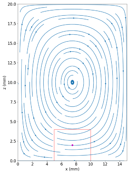
Figure 9: Magnetic field lines in the rectangular RF resonator with dimensions $a\times b\times d$=$15\times 10\times 20$mm along x,y,z respectively. The crystal (red square) sits at the bottom of the cavity and is crossed by the laser beam (magenta dot) propagating along y

At the position of the laser schematically represented in Fig.9 ($x=a/2$ and $z=2$ mm), the magnetic field is uniform (small beam side compared the cavity dimensions) and along $x$ with

$$B_{x}(z_{0})=-j\frac{E_{0}}{c}\frac{a}{\sqrt{d^{2}+a^{2}}}\cos\left(\frac{\pi z_{0}}{d}\right)$$ (41)

with $\displaystyle\cos\left(\frac{\pi z_{0}}{d}\right)\simeq 0.95$

The amplitude of the magnetic field can now be deduced from the incoming power $P_{\mathrm{rf}}$ and the resonator linewidth [41, Eq.(3.16)] and follows the resonant character of the energy stored. For an empty cavity (neglecting the spin cooperativity), we obtain

$$\mathbb{E}_{\mathrm{cav}}=\frac{\epsilon_{0}V}{8}E_{0}^{2}=\frac{4\kappa_{c}}{4\left(\omega_{\mathrm{rf}}-\omega_{c}\right)^{2}+\kappa_{t}^{2}}P_{\mathrm{rf}}$$ (42)

The spin interaction can also be introduced as in (3) where $W(\omega_{\mathrm{rf}})$ appears as an extra loss coefficient (spin absorption) or similarly as a rescaling of $\kappa_{t}$.

So the magnetic field amplitude in the crystal is

$$|B_{x}(z_{0})|=4\sqrt{\mu_{0}}\frac{a}{\sqrt{d^{2}+a^{2}}}\sqrt{\frac{P_{\mathrm{rf}}}{V}}\sqrt{\frac{2\kappa_{c}}{4\left(\omega_{\mathrm{rf}}-\omega_{c}\right)^{2}+\kappa_{t}^{2}}}$$ (43)

We have dropped the term $\displaystyle\cos\left(\frac{\pi z_{0}}{d}\right)$ for simplicity leading to a small 5% error. The expression can be further simplified, if needed, under critical coupling condition with $\kappa_{t}\approx 2\kappa_{c}$. Any way, the different parameters to determine to local value of the oscillating magnetic field are known for a given cavity geometry or measured from RF measurements detailed in 3.1.1.

The corresponding Rabi frequency, used to evaluate the electro-optics efficiency (6), finally reads as

$$\mu=\frac{g_{x}\mu_{B}|B_{x}(z_{0})|}{\hbar}=\frac{4g_{x}\mu_{B}}{\hbar}\sqrt{\mu_{0}}\frac{a}{\sqrt{d^{2}+a^{2}}}\sqrt{\frac{P_{\mathrm{rf}}}{V}}\sqrt{\frac{2\kappa_{c}}{4\left(\omega_{\mathrm{rf}}-\omega_{c}\right)^{2}+\kappa_{t}^{2}}}$$ (44)

where $g_{x}$ is $g$-factor along the $x$ direction of the RF field. In our case, the crystalline c-axis lies along $y$ (laser propagation) so $g_{x}=g_{\perp}$, the perpendicular value of the $g$-tensor.

Appendix C Estimation of the spin cooperativity

As introduced in section 3.1.1, the spin cooperativity can be deduced from the cavity parameters $\gamma$, $\kappa_{c}$ and spin coupling strength as

$$C_{\mu}=\frac{g_{\mu}^{2}N_{\mu}}{\gamma\kappa_{c}}$$ (45)

where $g_{\mu}$ is the coupling constant and $N_{\mu}$ the total number of spins. $g_{\mu}$ can be deduced for the single-photon Rabi frequency when $\mathbb{E}_{\mathrm{cav}}=\hbar\omega$.

The zero-point magnetic field fluctuations using the notation of section B then reads as

$$B_{\mathrm{vac}}=2\frac{a}{\sqrt{d^{2}+a^{2}}}\sqrt{\frac{2\hbar\omega\mu_{0}}{V}}$$ (46)

leading to the coupling strength $g_{\mu}=g_{x}\mu_{B}B_{\mathrm{vac}}/\hbar$

$$g_{\mu}=g_{x}\mu_{B}\frac{a}{\sqrt{d^{2}+a^{2}}}\sqrt{\frac{2\omega\mu_{0}}{\hbar V}}$$ (47)

As already noted in 4.2.2, because of the finite temperature and the imperfect spin polarization, we have to account for the population difference $\rho_{\mathrm{gg}}-\rho_{\mathrm{ss}}$ that scales the spin cooperativity as well, effectively modifying the number of spins $N_{\mu}\rightarrow\left(\rho_{\mathrm{gg}}-\rho_{\mathrm{ss}}\right)N_{\mu}$. At our temperature, we measure $\displaystyle\left(\rho_{\mathrm{gg}}-\rho_{\mathrm{ss}}\right)=0.12$ (see 4.2.2).

The cooperativity can now be evaluated for a 50 ppm doped sample, by knowing the Ca concentration ($1.3\times 10^{22}$ at/cm³) and noting that 77% of the erbium ions (without nuclear spin) are probed by our setup, we obtain $C_{\mu}=0.12$, in satisfying agreement the experimentally inferred value of 0.14 in section 3.1.1.

Appendix D Choice of the heterodyne beating frequency

One may be surprised by our choice of the heterodyne beating frequency that can be in principle arbitrarily taken within the detector bandwidth.

Indeed, when we record the noise spectrum on the photodiode, we interestingly observe a minimum close to 44 MHz that we choose as a beatnote heterodyne detection frequency as discussed in 2.2.

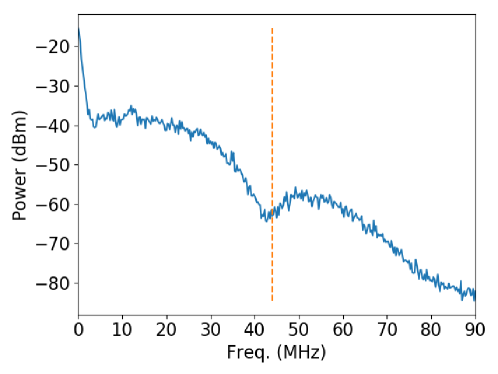
Figure 10: Noise spectrum on the photodiode (500 kHz resolution). We mark with a vertical dashed line the minimum close to 44 MHz that we choose as a beatnote heterodyne detection frequency for the transduction signal.

This minimum of the laser intensity noise that our partially fibered optical setup forms a Mach-Zender interferometer for the optical carrier (see Fig.2). The interferometer can be seen as a filter in the frequency domain, that exhibits minima for frequencies $\displaystyle\frac{c}{2L}$, $\displaystyle\frac{3c}{2L}$, $\displaystyle\frac{5c}{2L}$ … where $L$ is the optical path length difference between the two arms. This latter is approximately $3$m in our case, corresponding to the observed $44$ MHz minimum.

References

- [1] R. W. Andrews, R. W. Peterson, T. P. Purdy, K. Cicak, R. W. Simmonds, C. A. Regal, and K. W. Lehnert. Bidirectional and efficient conversion between microwave and optical light. Nature Physics, 10(4):321–326, March 2014.
- [2] Amit Vainsencher, K. J. Satzinger, G. A. Peairs, and A. N. Cleland. Bi-directional conversion between microwave and optical frequencies in a piezoelectric optomechanical device. Applied Physics Letters, 109(3):033107, 07 2016.
- [3] G.A. Peairs, M.-H. Chou, A. Bienfait, H.-S. Chang, C.R. Conner, É. Dumur, J. Grebel, R.G. Povey, E. Şahin, K.J. Satzinger, Y.P. Zhong, and A.N. Cleland. Continuous and time-domain coherent signal conversion between optical and microwave frequencies. Phys. Rev. Appl., 14:061001, Dec 2020.
- [4] Mohammad Mirhosseini, Alp Sipahigil, Mahmoud Kalaee, and Oskar Painter. Superconducting qubit to optical photon transduction. Nature, 588(7839):599–603, December 2020.
- [5] R. D. Delaney, M. D. Urmey, S. Mittal, B. M. Brubaker, J. M. Kindem, P. S. Burns, C. A. Regal, and K. W. Lehnert. Superconducting-qubit readout via low-backaction electro-optic transduction. Nature, 606(7914):489–493, June 2022.
- [6] William Hease, Alfredo Rueda, Rishabh Sahu, Matthias Wulf, Georg Arnold, Harald G.L. Schwefel, and Johannes M. Fink. Bidirectional electro-optic wavelength conversion in the quantum ground state. PRX Quantum, 1:020315, Nov 2020.
- [7] Rishabh Sahu, William Hease, Alfredo Rueda, Georg Arnold, Liu Qiu, and Johannes M. Fink. Quantum-enabled operation of a microwave-optical interface. Nature Communications, 13(1), March 2022.
- [8] R. Sahu, L. Qiu, W. Hease, G. Arnold, Y. Minoguchi, P. Rabl, and J. M. Fink. Entangling microwaves with light. Science, 380(6646):718–721, May 2023.
- [9] Georg Arnold, Thomas Werner, Rishabh Sahu, Lucky N. Kapoor, Liu Qiu, and Johannes M. Fink. All-optical single-shot readout of a superconducting qubit, 2023.
- [10] Nicholas J. Lambert, Alfredo Rueda, Florian Sedlmeir, and Harald G. L. Schwefel. Coherent conversion between microwave and optical photons—an overview of physical implementations. Advanced Quantum Technologies, 3(1):1900077, 2020.
- [11] Nikolai Lauk, Neil Sinclair, Shabir Barzanjeh, Jacob P Covey, Mark Saffman, Maria Spiropulu, and Christoph Simon. Perspectives on quantum transduction. Quantum Science and Technology, 5(2):020501, mar 2020.
- [12] Xu Han, Wei Fu, Chang-Ling Zou, Liang Jiang, and Hong X. Tang. Microwave-optical quantum frequency conversion. Optica, 8(8):1050–1064, Aug 2021.
- [13] Christopher O’Brien, Nikolai Lauk, Susanne Blum, Giovanna Morigi, and Michael Fleischhauer. Interfacing superconducting qubits and telecom photons via a rare-earth-doped crystal. Phys. Rev. Lett., 113:063603, Aug 2014.
- [14] Lewis A. Williamson, Yu-Hui Chen, and Jevon J. Longdell. Magneto-optic modulator with unit quantum efficiency. Phys. Rev. Lett., 113:203601, Nov 2014.
- [15] Jonathan R. Everts, Matthew C. Berrington, Rose L. Ahlefeldt, and Jevon J. Longdell. Microwave to optical photon conversion via fully concentrated rare-earth-ion crystals. Phys. Rev. A, 99:063830, Jun 2019.
- [16] D. E. Wortman. Optical Spectrum of Triply Ionized Erbium in Calcium Tungstate. The Journal of Chemical Physics, 54(1):314–321, 09 2003.
- [17] N Faure, C Borel, M Couchaud, G Basset, R Templier, and C Wyon. Optical properties and laser performance of neodymium doped scheelites CaWO4 and NaGd(WO4)2. Appl. Phys. B, 63(6):593–598, December 1996.
- [18] Thierry Chanelière, Gabriel Hétet, and Nicolas Sangouard. Chapter two - quantum optical memory protocols in atomic ensembles. volume 67 of Advances In Atomic, Molecular, and Optical Physics, pages 77 – 150. Academic Press, 2018.
- [19] AA Antipin, AN Katyshev, IN Kurkin, and L Ya Shekun. Paramagnetic resonance and spin-lattice relaxation of Er3+ and Tb3+ ions in crystal lattice of CaWO4. Soviet physics solid state, USSR, 10(2):468–+, 1968.
- [20] D.R. Mason and C. Kikuchi. Paramagnetic resonance of erbium in CaWO4. Physics Letters A, 28(4):260–261, 1968.
- [21] WB Mims. Phase memory in electron spin echoes, lattice relaxation effects in CaWO4: Er,Ce,Mn. Physical Review, 168(2):370, 1968.
- [22] S. Probst, G. Zhang, M. Rančić, V. Ranjan, M. Le Dantec, Z. Zhang, B. Albanese, A. Doll, R. B. Liu, J. Morton, T. Chanelière, P. Goldner, D. Vion, D. Esteve, and P. Bertet. Hyperfine spectroscopy in a quantum-limited spectrometer. Magnetic Resonance, 1(2):315–330, 2020.
- [23] Jake Rochman, Tian Xie, John G Bartholomew, KC Schwab, and Andrei Faraon. Microwave-to-optical transduction with erbium ions coupled to planar photonic and superconducting resonators. Nature Communications, 14(1):1153, 2023.
- [24] John G Bartholomew, Jake Rochman, Tian Xie, Jonathan M Kindem, Andrei Ruskuc, Ioana Craiciu, Mi Lei, and Andrei Faraon. On-chip coherent microwave-to-optical transduction mediated by ytterbium in YVO4. Nature communications, 11(1):3266, 2020.
- [25] Zong-Quan Zhou, Chao Liu, Chuan-Feng Li, Guang-Can Guo, Daniel Oblak, Mi Lei, Andrei Faraon, Margherita Mazzera, and Hugues de Riedmatten. Photonic integrated quantum memory in rare-earth doped solids. Laser & Photonics Reviews, 17(10):2300257, 2023.
- [26] Xavier Fernandez-Gonzalvo, Sebastian P. Horvath, Yu-Hui Chen, and Jevon J. Longdell. Cavity-enhanced raman heterodyne spectroscopy in Er3+:Y2SiO5 for microwave to optical signal conversion. Phys. Rev. A, 100:033807, Sep 2019.
- [27] J. Mlynek, N. C. Wong, R. G. DeVoe, E. S. Kintzer, and R. G. Brewer. Raman heterodyne detection of nuclear magnetic resonance. Phys. Rev. Lett., 50:993–996, Mar 1983.
- [28] M. Mitsunaga, E. S. Kintzer, and R. G. Brewer. Raman heterodyne interference: Observations and analytic theory. Phys. Rev. B, 31:6947–6957, Jun 1985.
- [29] S. K. Arora and B. Chudasama. Crystallization and optical properties of cawo4 and srwo4. Crystal Research and Technology, 41(11):1089–1095, 2006.
- [30] Francesco Cornacchia, Alessandra Toncelli, Mauro Tonelli, Elena Favilla, Kirill A. Subbotin, Valerii A. Smirnov, Denis A. Lis, and Evgenii V. Zharikov. Growth and spectroscopic characterization of Er3+:CaWO4. Journal of Applied Physics, 101(12):123113, 06 2007.
- [31] Nathalie Kunkel and Philippe Goldner. Recent advances in rare earth doped inorganic crystalline materials for quantum information processing. Zeitschrift für anorganische und allgemeine Chemie, 644(2):66–76, 2018.
- [32] Austin M Ferrenti, Nathalie P de Leon, Jeff D Thompson, and Robert J Cava. Identifying candidate hosts for quantum defects via data mining. Npj Comput. Mater., 6(1), August 2020.
- [33] Sylvain Bertaina, Serge Gambarelli, Alexandra Tkachuk, IN Kurkin, Boris Malkin, Anatole Stepanov, and Bernard Barbara. Rare-earth solid-state qubits. Nature nanotechnology, 2(1):39–42, 2007.
- [34] Marianne Le Dantec, Miloš Rančić, Sen Lin, Eric Billaud, Vishal Ranjan, Daniel Flanigan, Sylvain Bertaina, Thierry Chanelière, Philippe Goldner, Andreas Erb, Ren Bao Liu, Daniel Estève, Denis Vion, Emmanuel Flurin, and Patrice Bertet. Twenty-three–millisecond electron spin coherence of erbium ions in a natural-abundance crystal. Science Advances, 7(51):eabj9786, 2021.
- [35] Salim Ourari, Łukasz Dusanowski, Sebastian P Horvath, Mehmet T Uysal, Christopher M Phenicie, Paul Stevenson, Mouktik Raha, Songtao Chen, Robert J Cava, Nathalie P de Leon, and Jeff D Thompson. Indistinguishable telecom band photons from a single Er ion in the solid state. Nature, 620(7976):977–981, August 2023.
- [36] E. Billaud, L. Balembois, M. Le Dantec, M. Rančić, E. Albertinale, S. Bertaina, T. Chanelière, P. Goldner, D. Estève, D. Vion, P. Bertet, and E. Flurin. Microwave fluorescence detection of spin echoes. Phys. Rev. Lett., 131:100804, Sep 2023.
- [37] Zhiren Wang, Léo Balembois, Milos Rančić, Eric Billaud, Marianne Le Dantec, Alban Ferrier, Philippe Goldner, Sylvain Bertaina, Thierry Chanelière, Daniel Estève, Denis Vion, Patrice Bertet, and Emmanuel Flurin. Single electron-spin-resonance detection by microwave photon counting. Nature, 619(7969):276–281, 2023.
- [38] D.M. Pozar. Microwave Engineering. Addison-Wesley series in electrical and computer engineering. Addison-Wesley, 1990.
- [39] I. Diniz, S. Portolan, R. Ferreira, J. M. Gérard, P. Bertet, and A. Auffèves. Strongly coupling a cavity to inhomogeneous ensembles of emitters: Potential for long-lived solid-state quantum memories. Phys. Rev. A, 84:063810, Dec 2011.
- [40] B. Julsgaard and K. Mølmer. Reflectivity and transmissivity of a cavity coupled to two-level systems: Coherence properties and the influence of phase decay. Phys. Rev. A, 85:013844, Jan 2012.
- [41] Marianne Le Dantec. Electron spin dynamics of erbium ions in scheelite crystals, probed with superconducting resonators at millikelvin temperatures. Theses, Université Paris-Saclay, January 2022.
- [42] Bernal G. Enrique. Optical Spectrum and Magnetic Properties of Er3+ in CaWO4. The Journal of Chemical Physics, 55(5):2538–2549, September 1971.
- [43] Y Sun, C.W Thiel, R.L Cone, R.W Equall, and R.L Hutcheson. Recent progress in developing new rare earth materials for hole burning and coherent transient applications. Journal of Luminescence, 98(1):281–287, 2002. Proceedings of the Seventh International Meeting on Hole Burning, Single Molecules and Related Spectroscopies: Science and Applications.
- [44] AA Kaplyanskii and RM McFarlane. Spectroscopy of Crystals Containing Rare Earth Ions. Elsevier, 1987.
- [45] Guokui Liu and Bernard Jacquier. Spectroscopic properties of rare earths in optical materials, volume 83. Springer Science & Business Media, 2006.
- [46] Stephen C. Rand. Lectures on Light: Nonlinear and Quantum Optics using the Density Matrix. Oxford University Press, 06 2016.
- [47] Paul R. Berman and Vladimir S. Malinovsky. Principles of Laser Spectroscopy and Quantum Optics. Princeton University Press, 2011.
- [48] Alexey V. Gorshkov, Axel André, Mikhail D. Lukin, and Anders S. Sørensen. Photon storage in -type optically dense atomic media. ii. free-space model. Phys. Rev. A, 76:033805, Sep 2007.
- [49] Tian Xie, Jake Rochman, John G. Bartholomew, Andrei Ruskuc, Jonathan M. Kindem, Ioana Craiciu, Charles W. Thiel, Rufus L. Cone, and Andrei Faraon. Characterization of Er3+:YVO4 for microwave to optical transduction. Phys. Rev. B, 104:054111, Aug 2021.
- [50] Andrew JM Kiruluta. Field propagation phenomena in ultra high field NMR: A Maxwell–Bloch formulation. Journal of Magnetic Resonance, 182(2):308–314, 2006.
- [51] Mikael Afzelius, Matthias U. Staudt, Hugues de Riedmatten, Nicolas Gisin, Olivier Guillot-Noël, Philippe Goldner, Robert Marino, Pierre Porcher, Enrico Cavalli, and Marco Bettinelli. Efficient optical pumping of zeeman spin levels in Nd3+:YVO4. Journal of Luminescence, 130(9):1566–1571, 2010. Special Issue based on the Proceedings of the Tenth International Meeting on Hole Burning, Single Molecule, and Related Spectroscopies: Science and Applications (HBSM 2009) - Issue dedicated to Ivan Lorgere and Oliver Guillot-Noel.
- [52] B.W. Shore. Manipulating Quantum Structures Using Laser Pulses. Cambridge University Press, 2011.