Covering one point process with another

Abstract

Let $X_{1},X_{2},\ldots$ and $Y_{1},Y_{2},\ldots$ be i.i.d. random uniform points in a bounded domain $A\subset\mathbb{R}^{2}$ with smooth or polygonal boundary. Given $n,m,k\in\mathbb{N}$, define the two-sample $k$-coverage threshold $R_{n,m,k}$ to be the smallest $r$ such that each point of $\{Y_{1},\ldots,Y_{m}\}$ is covered at least $k$ times by the disks of radius $r$ centred on $X_{1},\ldots,X_{n}$. We obtain the limiting distribution of $R_{n,m,k}$ as $n\to\infty$ with $m=m(n)\sim\tau n$ for some constant $\tau>0$, with $k$ fixed. If $A$ has unit area, then $n\pi R_{n,m(n),1}^{2}-\log n$ is asymptotically Gumbel distributed with scale parameter $1$ and location parameter $\log\tau$. For $k>2$, we find that $n\pi R_{n,m(n),k}^{2}-\log n-(2k-3)\log\log n$ is asymptotically Gumbel with scale parameter $2$ and a more complicated location parameter involving the perimeter of $A$; boundary effects dominate when $k>2$. For $k=2$ the limiting cdf is a two-component extreme value distribution with scale parameters 1 and 2. We also give analogous results for higher dimensions, where the boundary effects dominate for all $k$.

1 Introduction

This paper is primarily concerned with the following two-sample random coverage problem. Given a specified compact region $B$ in a $d$-dimensional Euclidean space, suppose $m$ points $Y_{j}$ are placed randomly in $B$. What is the probability that these $m$ points are fully covered by a union of Euclidean balls of radius $r$ centred on $n$ points $X_{i}$ placed independently uniformly at random in $B$, in the large-$n$ limit with $m=m(n)$ becoming large and $r=r(n)$ becoming small in an appropriate manner?

In an alternative version of this question, the $X$-points are placed uniformly not in $B$, but in a larger region $A$ with $B\subset A^{o}$ ($A^{o}$ denotes the interior of $A$). This version is simpler because boundary effects are avoided. We consider this version too.

We shall express our results in terms of the two-sample coverage threshold $R_{n,m}$, which we define to be the the smallest radius of balls, centred on a set $\mathcal{X}_{n}$ of $n$ independent uniform random points in $A$, required to cover all the points of a sample ${\cal Y}_{m}$ of $m$ uniform random points in $B$. More generally, for $k\in\mathbb{N}$ the two-sample $k$-coverage threshold $R_{n,m,k}$ is the smallest radius required to cover ${\cal Y}_{m}$ $k$ times. These thresholds are random variables, because the locations of the centres are random. We investigate their probabilistic behaviour as $n$ and $m$ become large.

A related question is to ask for coverage of the whole set $B$, not just of the point set ${\cal Y}_{m}$. We refer here to the smallest radius $r$ such that $B$ is contained in the union of the balls of radius $r$ centred on points of $A$, as the complete coverage threshold. The asymptotic behaviour of this threshold has been addressed in [2] and [4] (for the case with $B\subset A^{o}$) and in [8] (for the case with $B=A$). Clearly $R_{n,m}$ provides a lower bound for the complete coverage threshold.

Also related is the problem, when $m=n$ and $B=A$, of finding the matching threshold, that is, the minimum $r$ such that a perfect bipartite matching of the samples $\mathcal{X}_{n}$ and ${\cal Y}_{n}$ exists with all edges of length at most $r$. This problem has been considered in [6, 11], with applications to the theory of empirical measures. See e.g. [1] for recent application of results in [6, 11] to clustering and classification problems in machine-learning algorithms.

Our problem is different since we allow the $X$-points to practice polygamy, and require all of the $Y$-points, but not necessarily all of the $X$-points, to be matched. Clearly $R_{n,n}$ is a lower bound for the matching threshold. This lower bound is asymptotically of a different order of magnitude than the matching threshold when $d=2$, but the same order of magnitude when $d\geq 3$. A slightly better lower bound is given by $\tilde{R}_{n,n}$, which we define to be the smallest $r$ such that all $Y$-points are covered by $X$-points and all $X$-points are covered by $Y$-points. We expect that our methods can be used to show that $\lim_{n\to\infty}\mathbb{P}[\tilde{R}_{n,n}\leq r_{n}]=\lim_{n\to\infty}\mathbb{P}[R_{n,n}\leq r_{n}]^{2}$ for any sequence $(r_{n})$ such that the limit exists, but proving this is beyond the scope of this paper. It is tempting to conjecture that the lower bound $\tilde{R}_{n,n}$ for the matching threshold might perhaps be asymptotically sharp as $n\to\infty$ in sufficiently high dimensions.

Another related problem is that of understanding the bipartite connectivity threshold. Given $\mathcal{X}_{n},{\cal Y}_{m}$ and $r>0$, we can create a bipartite random geometric graph (BRGG) on vertex set $\mathcal{X}_{n}\cup{\cal Y}_{m}$ by drawing an edge between any pair of points $x\in\mathcal{X}_{n},y\in{\cal Y}_{m}$ a distance at most $r$ apart. The bipartite connectivity threshold is the smallest $r$ such that this graph is connected, and the two-sample coverage threshold $R_{n,m}$ is a lower bound for the bipartite connectivity threshold. Two related thresholds are: the smallest $r$ such that each point of ${\cal Y}_{m}$ is connected by a path in the BRGG to at least one other point of ${\cal Y}_{m}$, and the smallest $r$ such that any two points of ${\cal Y}_{m}$, are connected by a path in the BRGG (but isolated points in $\mathcal{X}_{n}$ are allowed in both cases). Provided $m\geq 2$, these thresholds both lie between $R_{n,m}$ and the bipartite connectivity threshold, and have been studied in [3, 7].

Motivation for considering coverage problems comes from wireless communications technology (among other things); one may be interested in covering a region of land by mobile wireless transmitters (with locations modelled as the set of random points $X_{i}$). If interested in covering the whole region of land, one needs to consider the complete coverage threshold. In practice, however, it may be sufficient to cover not the whole region but a finite collection of receivers placed in that region (with locations modelled as the set of random points $Y_{j}$), and the two-sample coverage threshold addresses this problem. See [3] for further discussion of motivation from wireless communications.

We shall determine the limiting behaviour of $\mathbb{P}[R_{n,m(n),k}\leq r_{n}]$ for any fixed $k$, any sequence $m(n)_{n\geq 1}$ of integers asymptotically proportional to $n$, and any sequence of numbers $(r_{n})$ such that the limit exists, for the case where $B$ is smoothly bounded (for general $d\geq 2$) or where $B$ is a polygon (for $d=2$). We also obtain similar results for the Poissonized versions of this problem.

Our results show that when $d\geq 3$ the boundary effects dominate, i.e. the point of the ${\cal Y}$-sample furthest from its $k$-nearest neighbour in the $\mathcal{X}$-sample is likely to be near the boundary of $B$. When $d=2$, boundary effects are negligible for $k=1$ but dominate for $k\geq 3$. When $d=k=2$ the boundary and interior effects are of comparable importance; the point of the ${\cal Y}$-sample furthest from its second-nearest neighbour in the $\mathcal{X}$-sample has non-vanishing probability of being near the boundary of $B$ but also non-vanishing probability of being in the interior.

In Section 6 we discuss the results of computer experiments, in which we sampled many independent copies of $R_{n,m(n),k}$ and plotted the estimated distributions of these radii (suitably transformed so that a weak law holds) alongside the limiting distributions we state in Section 2. These experiments motivated a refinement to our limit results, in which we explicitly included the leading-order error term, so that we can approximate the distribution of $R_{n,m(n),k}$ well for given finite $n$.

We work within the following mathematical framework. Let $d\in\mathbb{N}$. Let $A\subset\mathbb{R}^{d}$ be compact. Let $B\subset A$ be a specified Borel set (possibly the set $A$ itself) with a nice boundary (in a sense to be made precise later on), and with volume $|B|>0$. Suppose on some probability space $(\mathbb{S},{\cal F},\mathbb{P})$ that $X_{1},Y_{1},X_{2},Y_{2},\ldots$ are independent random $d$-vectors with $X_{i}$ uniformly distributed over $A$ and $Y_{i}$ uniformly distributed over $B$ for each $i\in\mathbb{N}$. For $x\in\mathbb{R}^{d}$ and $r>0$ set $B_{r}(x):=B(x,r):=\{y\in\mathbb{R}^{d}:\|y-x\|\leq r\}$ where $\|\cdot\|$ denotes the Euclidean norm. For $n\in\mathbb{N}$, let $\mathcal{X}_{n}:=\{X_{1},\ldots,X_{n}\}$ and let ${\cal Y}_{n,B}:=\{Y_{1},\ldots,Y_{n}\}$. Given also $m,k\in\mathbb{N}$, we define the $k$-coverage threshold $R_{n,m,k}$ by

$$R_{n,m,k}(B):=\inf\left\{r>0:\mathcal{X}_{n}(B(y,r))\geq k~{}~{}~{}~{}\forall y\in{\cal Y}_{m,B}\right\},~{}~{}~{}n,m,k\in\mathbb{N},$$ (1.1)

where for any point set $\mathcal{X}\subset\mathbb{R}^{d}$ and any $D\subset\mathbb{R}^{d}$ we write $\mathcal{X}(D)$ for the number of points of $\mathcal{X}$ in $D$, and we use the convention $\inf\{\}:=+\infty$. In particular $R_{n,m}(B):=R_{n,m,1}(B)$ is the two-sample coverage threshold. Observe that $R_{n,m}(B)=\inf\{r>0:{\cal Y}_{m,B}\subset\cup_{i=1}^{n}B(X_{i},r)\}$.

We are mainly interested in the case with $B=A$. In this case we write simply ${\cal Y}_{m}$, $R_{n,m,k}$ and $R_{n,m}$ for ${\cal Y}_{m,A}$, $R_{n,m,k}(A)$ and $R_{n,m}(A)$ respectively.

We are interested in the asymptotic behaviour of $R_{n,m}(B)$ for large $n,m$; in fact we take $m$ to be asymptotically proportional to $n$. More generally, we consider $R_{n,m,k}(B)$ for fixed $k\in\mathbb{N}$.

We also consider analogous quantities denoted $R^{\prime}_{t,u}(B)$ and $R^{\prime}_{t,u,k}(B)$ respectively, defined similarly using Poisson samples of points. To define these formally, let $(Z_{t},t\geq 0)$ be a unit rate Poisson counting process, independent of $(X_{1},Y_{1},X_{2},Y_{2},\ldots)$ and on the same probability space $(\mathbb{S},{\cal F},\mathbb{P})$ (so $Z_{t}$ is Poisson distributed with mean $t$ for each $t>0$). Let $(Z^{\prime}_{t},t\geq 0)$ be a second unit rate Poisson counting process, independent of $(X_{1},Y_{1},X_{2},Y_{2},\ldots)$ and of $(Z_{t},t\geq 0)$. The point process ${\cal P}_{t}:=\{X_{1},\ldots,X_{Z_{t}}\}$ is a Poisson point process in $\mathbb{R}^{d}$ with intensity measure $t\mu$, where we set $\mu$ to be the uniform distribution over $A$ (see e.g. [5]). The point process ${\cal Q}_{t,B}:=\{Y_{1},\ldots,Y_{Z^{\prime}_{t}}\}$ is a Poisson point process in $\mathbb{R}^{d}$ with intensity measure $t\nu$, where we set $\nu$ to be the uniform distribution over $B$. Then for $t,u\in(0,\infty),k\in\mathbb{N}$ we define

$$R^{\prime}_{t,u,k}(B):=\inf\left\{r>0:{\cal P}_{t}(B(y,r))\geq k~{}\forall y\in{\cal Q}_{u,B}\right\},$$ (1.2)

with $R^{\prime}_{t,u}:=R^{\prime}_{t,u,1}$. When $B=A$ we write simply ${\cal Q}_{t}$, $R^{\prime}_{t,u,k}$, $R^{\prime}_{t,u}$, for ${\cal Q}_{t,A}$, $R^{\prime}_{t,u,k}(A)$, $R^{\prime}_{t,u,k}(A)$, respectively.

We mention some notation used throughout. For $D\subset\mathbb{R}^{d}$, let $\overline{D}$ denote the closure of $D$. Let $|D|$ denote the Lebesgue measure (volume) of $D$, and $|\partial D|$ the perimeter of $D$, i.e. the $(d-1)$-dimensional Hausdorff measure of $\partial D$, when these are defined. Given $t>1$, we write $\log\log t$ for $\log(\log t)$. Let $o$ denote the origin in $\mathbb{R}^{d}$.

Let $\theta_{d}$ denote the volume of a unit radius ball in $\mathbb{R}^{d}$. Set $f_{0}:=1/|A|$.

If $t_{0}\in(0,\infty)$ and $f(t),g(t)$ are two functions, defined for all $t\geq t_{0}$ with $g(t)>0$ for all $t\geq t_{0}$, the notation $f(t)=O(g(t))$ as $t\to\infty$ means that $\limsup_{t\to\infty}(|f(t)|/g(t))<\infty$, and the notation $f(t)=o(g(t))$ as $t\to\infty$ means that $\limsup_{t\to\infty}(|f(t)|/g(t))=0.$ If also $f(t)>0$ for all $n\geq n_{0}$, we use notation $f(t)=\Theta(g(t))$ to mean that both $f(t)=O(g(t)$ and $g(t)=O(f(t))$.

2 Statement of results

Our results are concerned with weak convergence for $R_{n,m,k}(B)$ (defined at (1.1)) as $n\to\infty$ with $k$ fixed and $m$ asymptotically proportional to $n$. We also give similar results for $R^{\prime}_{t,\tau t,k}$, defined at (1.2), as $t\to\infty$ with $\tau>0$ also fixed. In all of these limiting results we are taking the variable $n$ to be integer-valued and $t$ to be real-valued.

Recall that our $\mathcal{X}$-sample is of points uniformly distributed over a compact region $A\subset\mathbb{R}^{d}$, and the ${\cal Y}$-sample is of points in $B$, where $B\subset A$ has a ‘nice’ boundary. We now make this assumption more precise. We always assume one of the following:

A1: $d\geq 2$ and $B=A$ and $A$ has a $C^{2}$ boundary and $\overline{A^{o}}=A$, or

A2: $d=2$ and $B=A$ and $A$ is polygonal, or

A3: $d\geq 2$ and $\overline{B}\subset A^{o}$, and $B$ is Riemann measurable with $|B|>0$. (Recall that a compact set $B$ is said to be Riemann measurable if $|\partial B|=0$.)

We say that $A$ has a $C^{2}$ boundary if for each $x\in\partial A$ there exists a neighbourhood $U$ of $x$ and a real-valued function $f$ that is defined on an open set in $\mathbb{R}^{d-1}$ and twice continuously differentiable, such that $\partial A\cap U$, after a rotation, is the graph of the function $f$. The extra condition $\overline{A^{o}}=A$ should also have been included in [8] to rule out examples such as the union of a disk and a circle in $\mathbb{R}^{2}$.

For compact $A\subset\mathbb{R}^{d}$ satisfying A1 or A2, let $|A|$ denote the volume (Lebesgue measure) of $A$ and $|\partial A|$ the perimeter of $A$, i.e. the $(d-1)$-dimensional Hausdorff measure of $\partial A$, the topological boundary of $A$. Also define

$$\sigma_{A}:=\frac{|\partial A|}{|A|^{1-1/d}}.$$ (2.1)

Note that $\sigma_{A}$ is invariant under scaling of $A$, and is at least $d\theta_{d}^{1/d}$ by the isoperimetric inequality. Sometimes $\sigma_{A}^{d}$ is called the isoperimetric ratio of $A$.

Our first result concerns the case with $\overline{B}\subset A^{o}$. Recall that $f_{0}:=1/|A|$.

Theorem 2.1 (Fluctuations of $R_{n,m,k}(B)$ when $\overline{B}\subset A^{o}$).

Suppose A3 applies. Let $k\in\mathbb{N}$ and $\tau>0,\beta\in\mathbb{R}$. Let $m:\mathbb{N}\to\mathbb{N}$, and assume $\tau_{n}:=m(n)/n\to\tau$ as $n\to\infty$. Then as $n\to\infty$ we have

$$\mathbb{P}[n\theta_{d}f_{0}R_{n,m(n),k}(B)^{d}-\log n-(k-1)\log\log n\leq\beta]$$

$$~{}~{}~{}~{}=\exp\left(-\frac{\tau_{n}e^{-\beta}(k-1)^{2}\log\log n}{(k-1)!\log n}\right)e^{-(\tau_{n}e^{-\beta})/(k-1)!}+O((\log n)^{-1}).$$ (2.2)

Also as $t\to\infty$ we have

$$\mathbb{P}[t\theta_{d}f_{0}(R^{\prime}_{t,\tau t,k}(B))^{d}-\log t-(k-1)\log\log t\leq\beta]$$

$$~{}~{}~{}~{}=\exp\left(-\frac{\tau e^{-\beta}(k-1)^{2}\log\log t}{(k-1)!\log t}\right)e^{-(\tau e^{-\beta})/(k-1)!}+O((\log t)^{-1}).$$ (2.3)

Remarks. 1. Given $\xi\in\mathbb{R}$, $\theta\in(0,\infty)$, let ${\mathsf{Gu}}_{\xi,\theta}$ denote a Gumbel random variable with location parameter $\xi$ and scale parameter $\theta$, i.e. with cumulative distribution function (cdf) $F(x)=\exp(-e^{-(x-\xi)/\theta})$. Since the right hand side of (2.2) converges to $\exp(-(\tau e^{-\beta})/(k-1)!)$ as $n\to\infty$, it follows from (2.2) that as $n\to\infty$ we have the convergence in distribution:

$$n\theta_{d}f_{0}R_{n,m(n),k}(B)^{d}-\log n-(k-1)\log\log n\stackrel{{\scriptstyle{\cal D}}}{{\longrightarrow}}{\mathsf{Gu}}_{\log(\tau/(k-1)!),1}.$$

Similarly, as $t\to\infty$, by (2.3) we have

$$n\theta_{d}f_{0}R^{\prime}_{t,\tau t,k}(B)^{d}-\log t-(k-1)\log\log t\stackrel{{\scriptstyle{\cal D}}}{{\longrightarrow}}{\mathsf{Gu}}_{\log(\tau/(k-1)!),1}.$$

2. The $O((\log n)^{-1})$ term in (2.2) and the $O((\log t)^{-1})$ term in (2.3) come partly from an error bound of $O((\log t)^{1-d})$ in a Poisson approximation for the number of isolated points; see Lemma 4.1. If $d\geq 3$ the error bound in the Poisson approximation is of higher order, and hence we can give a more accurate approximation with an explicit $(\log n)^{-1}$ term (respectively, $(\log t)^{-1}$ term) included in the first exponential factor on the right, and an error of $O((\frac{\log\log n}{\log n})^{2})$ in (2.2) (resp., of $O((\frac{\log\log t}{\log t})^{2})$ in (2.3)). See (5.2) and (5.3) in the proof of Theorem 2.1 for details.

All of our remaining results are for the case $B=A$.

First we briefly discuss the case where $A$ is the $d$-dimensional unit torus. (and $B=A$). In this case, taking $f_{0}=1$, we can obtain exactly the same result as stated in Theorem 2.1, by the same proof. We note that a result along these lines (for $k=1$ only) has been provided previously (with a different proof) in [3, Theorem 3.2], for $\tau$ large. [3] is more concerned with the threshold $r$ such that each vertex of ${\cal Y}_{m}$ has a path to at least one other point of ${\cal Y}_{m}$ in the BRGG. In any event, the authors of [3] explicitly restrict attention to the torus, in their words, to ‘nullify some of the technical complications arising out of boundary effects’. In our next results, we embrace these technical complications.

We next give our main result for $d=2$, $k=1$.

Theorem 2.2 (Fluctuations of $R_{n,m}$ in a planar region with boundary).

Suppose $d=2$ and A1 or A2 holds. Set $f_{0}:=|A|^{-1}$. Let $\beta,\tau\in\mathbb{R}$ with $\tau>0$. Suppose $m:\mathbb{N}\to\mathbb{N}$ with $\tau_{n}:=m(n)/n\to\tau$ as $n\to\infty$. Then as $n\to\infty$

$$\mathbb{P}\left[n\pi f_{0}R_{n,m(n)}^{2}-\log n\leq\beta\right]=\exp\Big{(}-\frac{\tau_{n}\pi^{1/2}\sigma_{A}e^{-\beta/2}}{2(\log n)^{1/2}}\Big{)}e^{-\tau_{n}e^{-\beta}}+O((\log n)^{-1}).$$ (2.4)

Also, as $t\to\infty$,

$$\mathbb{P}\left[t\pi f_{0}(R^{\prime}_{t,\tau t})^{2}-\log t\leq\beta\right]=\exp\Big{(}-\frac{\tau\pi^{1/2}\sigma_{A}e^{-\beta/2}}{2(\log t)^{1/2}}\Big{)}\exp\left(-\tau e^{-\beta}\right)+O((\log t)^{-1}).$$ (2.5)

Remark. It follows from (2.4) that $n\pi f_{0}R_{n,m(n)}^{2}-\log n\stackrel{{\scriptstyle{\cal D}}}{{\longrightarrow}}{\mathsf{Gu}}_{\log\tau,1}$. Denoting the median of the distribution of any continuous random variable $Z$ by $\mu(Z)$, we have $\mu(n\pi f_{0}R_{n,m(n)}^{2})=\log n+\mu({\mathsf{Gu}}_{\log\tau,1})+o(1)$. We can subtract the medians from both sides, and then we have $n\pi f_{0}R_{n,m(n)}^{2}-\mu(n\pi f_{0}R_{n,m(n)}^{2})\stackrel{{\scriptstyle{\cal D}}}{{\longrightarrow}}{\mathsf{Gu}}_{\log\log 2,1}$, where ${\mathsf{Gu}}_{\log\log 2,1}$ is a Gumbel random variable with scale parameter 1 and median 0. The second row of Figure 2 illustrates each of these two convergences in distribution. It is clearly visible that subtracting the median gives a much smaller discrepancy between the distribution of $n\pi f_{0}R_{n,m(n)}^{2}-\mu(n\pi f_{0}R_{n,m(n)}^{2})$ and its limit, suggesting that $\mu(n\pi f_{0}R_{n,m(n)}^{2})-\log n\to\mu({\mathsf{Gu}}_{\log\tau,1})$ quite slowly. However, we estimated $\mu(n\pi f_{0}R_{n,m(n)}^{2})$ using the sample median of a large number of independent copies of $n\pi f_{0}R_{n,m(n)}^{2}$. When applying estimates such as (2.4) to real data, a large number of samples may not be available, and we do not currently have an expression for $\mu(n\pi f_{0}R_{n,m(n)}^{2})-\log n-\mu({\mathsf{Gu}}_{\log\tau,1})$.

Simulations with $A$ taken to be a disk or square suggest that even for quite large values of $n$, with $m(n)=\lfloor\tau n\rfloor$ for some fixed $\tau$, the estimated cdf of $n\pi f_{0}R_{n,m(n)}^{2}-\log n$ from simulations does not match the limiting Gumbel cdf particularly well. This can be seen in the bottom-left plot of Figure 2, where the estimated cdf (the blue curve) is not well-approximated by the limit (the black dashed curve). This is because the multiplicative correction factor of $\exp(-\tau_{n}(\pi^{1/2}/2)\sigma_{A}e^{-\beta/2}(\log n)^{-1/2})$, which we see in (2.4), tends to 1 very slowly. (We have written it as a multiplicative correction to ensure that the right hand side is a genuine cdf in $\tau_{n}$ plus an $O((\log n)^{-1})$ error term.)

If instead we compare the cdf of $n\pi f_{0}R_{n,m(n)}^{2}$ estimated by simulations with the corrected cdf $F(x)=\exp(-\frac{\tau_{n}\sigma_{A}e^{-x/2}}{(\log n)^{1/2}})\exp(-\tau_{n}e^{-x})$, illustrated as a red dotted line in the same part of Figure 2, we get a much better match.

Next we give results for $d=2,k\geq 2$ and for $d\geq 3$. Given $(d,k)$ we define the constant

$$c_{d,k}:=\frac{\theta_{d}^{1-1/d}(1-1/d)^{k-2+1/d}}{(k-1)!2^{1-1/d}\theta_{d-1}},$$ (2.6)

Theorem 2.3.

Suppose A1 or A2 holds. Let $\beta,\tau\in\mathbb{R}$ with $\tau>0$. Suppose $m:\mathbb{N}\to\mathbb{N}$ with $\tau_{n}:=m(n)/n\to\tau$ as $n\to\infty$, and for $n\in\mathbb{N}$, $t>0$ let

$$u_{n}:=\mathbb{P}[n\theta_{d}f_{0}R_{n,m(n),k}^{d}-(2-2/d)\log n-(2k-4+2/d)\log\log n)\leq\beta];$$

$$u^{\prime}_{t}:=\mathbb{P}[t\theta_{d}f_{0}(R^{\prime}_{t,\tau t,k})^{d}-(2-2/d)\log t-(2k-4+2/d)\log\log t)\leq\beta].$$

If $(d,k)=(2,2)$ then as $n\to\infty$,

$$u_{n}=\exp\Big{(}-\frac{\tau_{n}\pi^{1/2}\sigma_{A}e^{-\beta/2}\log\log n}{8\log n}\Big{)}\exp\left(-\tau_{n}\left(e^{-\beta}+\frac{\pi^{1/2}\sigma_{A}e^{-\beta/2}}{4}\right)\right)+O\big{(}\frac{1}{\log n}\big{)},$$ (2.7)

and as $t\to\infty$,

$$u^{\prime}_{t}=\exp\Big{(}-\frac{\tau_{n}\pi^{1/2}\sigma_{A}e^{-\beta/2}\log\log t}{8\log t}\Big{)}\exp\left(-\tau\left(e^{-\beta}+\frac{\pi^{1/2}\sigma_{A}e^{-\beta/2}}{4}\right)\right)+O\big{(}\frac{1}{\log t}\big{)}.$$ (2.8)

If $d=2,k\geq 3$ or if $d\geq 3$ then as $n\to\infty$,

$$u_{n}=\exp\Big{(}-\frac{c_{d,k}\tau_{n}\sigma_{A}e^{-\beta/2}(k-2+1/d)^{2}\log\log n}{(1-1/d)\log n}\Big{)}\exp\left(-c_{d,k}\tau_{n}\sigma_{A}e^{-\beta/2}\right)$$

$$+O\Big{(}\frac{1}{\log n}\Big{)}$$ (2.9)

and as $t\to\infty$,

$$u^{\prime}_{t}=\exp\Big{(}-\frac{c_{d,k}\tau\sigma_{A}e^{-\beta/2}(k-2+1/d)^{2}\log\log t}{(1-1/d)\log t}\Big{)}\exp\left(-c_{d,k}\tau\sigma_{A}e^{-\beta/2}\right)$$

$$+O\Big{(}\frac{1}{\log t}\Big{)}.$$ (2.10)

Remarks. 1. It follows from (2.9), (2.10) that when $d=2,k\geq 3$ or $d\geq 3$ we have as $n\to\infty$ that

$$n\theta_{d}f_{0}R_{n,m(n),k}^{d}-(2-2/d)\log n-(2k-4+2/d)\log\log n\stackrel{{\scriptstyle{\cal D}}}{{\longrightarrow}}{\mathsf{Gu}}_{\log(c_{d,k}\tau\sigma_{A}),2},$$

along with a similar result for $R_{t,\tau t,k}$. On the other hand, when $d=2,k=2$ we have from (2.7) that

$$n\pi f_{0}R_{n,m(n),2}^{2}-\log n-\log\log n\stackrel{{\scriptstyle{\cal D}}}{{\longrightarrow}}\max({\mathsf{Gu}}_{\log\tau,1},{\mathsf{Gu}}^{\prime}_{\log(\tau\pi^{1/2}\sigma_{A}/4),2}),$$

where ${\mathsf{Gu}}$ and ${\mathsf{Gu}}^{\prime}$ denote two independent Gumbel variables with the parameters shown. The distribution of the maximum of two independent Gumbel variables with different scale parameters is known as a two-component extreme value (TCEV) distribution in the hydrology literature [10].

2. As in the case of Theorem 2.1, when $d\geq 3$ in Theorem 2.3 we could replace the $O((\log n)^{-1})$ remainder in (2.9) with an explicit $(\log n)^{-1}$ term and an $O((\frac{\log\log n}{\log n})^{2})$ remainder, and likewise for the $O((\log t)^{-1})$ remainder in (2.10); see (5.39) and (5.38) in the proof of Theorem 2.3 for details.

Comparing these results with the corresponding results for the complete coverage threshold [2, 4, 8], we find that the typical value of that threshold (raised to the power $d$ and then multiplied by $n$) is greater than the typical value of our two-sample coverage threshold (transformed the same way) by a constant multiple of $\log\log n$. For example, our Theorem 2.1 has a coefficient of $k-1$ for $\log\log n$ while [8, Proposition 2.4] has a coefficient of $k$. When $d=2,k=1$, our Theorem 2.2 has a coefficient of zero for $\log\log n$ whereas [8, Theorem 2.2] has a coefficient of $1/2$.

We shall prove our theorems using the following strategy. Fix $k\in\mathbb{N}$. Given $t,r>0$ define the random ‘vacant’ set

$$V_{t,r,k}:=\{x\in A:{\cal P}_{t}(B(x,r))<k\}.$$ (2.11)

Given $\gamma\in(0,\infty)$, suppose we can find $(r_{t})_{t>0}$ such that $t\mathbb{E}\,[|V_{t,r_{t},k}\cap B|]/|B|=\gamma$. If we know $t|V_{t,r_{t},k}\cap B|/|B|\approx\gamma$, then the distribution of ${\cal Q}_{\tau t,B}(V_{t,r_{t},k})$ is approximately Poisson with mean $\tau\gamma$, and we use the Chen-Stein method to make this Poisson approximation quantitative, and hence show that $\mathbb{P}[R^{\prime}_{t,\tau t,k}\leq r_{t}]$ approximates to $e^{-\tau\gamma}$ for $t$ large (see Lemma 4.1). By coupling binomial and Poisson point processes, we obtain a similar result for $\mathbb{P}[R_{n,m(n),k}\leq r_{n}]$ (see Lemma 4.2).

Finally, we need to find nice limiting expression for $r_{t}$ as $t\to\infty$. By Fubini’s theorem $\mathbb{E}\,[|V_{t,r_{t},k}\cap B|]=\int_{B}p_{t}(x)dx$, where we set $p_{t}(x)=\mathbb{P}[x\in V_{t,r_{t},k}]$. Hence we need to take $r_{t}\to 0$. Under A3, for $t$ large $p_{t}(x)$ is constant over $x\in B$ so finding a limiting expression for $r_{t}$ in that case is fairly straightforward.

Under Assumption A1 or A2, we need to deal with boundary effects since $p_{t}(x)$ is larger for $x$ near the boundary of $A$ than in the interior (or ‘bulk’) of $A$. In Lemma 3.3 we determine the asymptotic behaviour of the integral near a flat boundary; since the contribution of corners turns out to be negligible this enables us to handle the boundary contribution under A2.

To deal with the curved boundary of $A$ under Assumption A1, we adapt a method that was developed in [8] to understand the complete coverage threshold. We approximate to $A$ by a polygon (or in higher dimensions, a polytope) $A_{t}$ with spacing that tends to zero more slowly than $r_{t}$, and deal with the integral near the flat parts of $\partial A_{t}$ using Lemma 3.3 again.

It turns out that $d=2,k=1$ is a special case because in this case only, the contribution of the bulk dominates the contribution of the boundary region to $\mathbb{E}\,[|V_{t,r_{t},k}|]$. When $d=2,k=2$ both contributions are equally important, and in all other cases the boundary contribution dominates the contribution of the bulk. This is why the formula for the centring constant for $R^{\prime}_{t,\tau t,k}$ or $R_{n,m,k}$ in terms of $d$ and $k$ is different for Theorem 2.2 than for Theorem 2.3 (the coefficient of $\log\log n$ being 0 rather than 1 in Theorem 2.2), and why in Theorem 2.3 the limiting distribution is TCEV for $d=k=2$ but is Gumbel for all other cases.

3 Preparatory lemmas

We use the following notation from time to time. Given $r>0$, and $\Gamma\subset\mathbb{R}^{d}$, set $\Gamma^{(r)}:=\cup_{x\in\Gamma}B_{r}(x)$. Given also $A\subset\mathbb{R}^{d}$, set $A^{(-r)}:=A\setminus(\partial A)^{(-r)}$.

Let $\pi:\mathbb{R}^{d}\to\mathbb{R}^{d-1}$ denote projection onto the first $d-1$ coordinates and let $h:\mathbb{R}^{d}\to\mathbb{R}$ denote projection onto the last coordinate ($h$ stands for ‘height’).

3.1 Geometrical lemmas

In Lemma 3.2 below we give lower bounds on the volume within $A$ of a ball, and of the difference between two balls, having their centres near the boundary of $A$.

In proving these lemmas, we let $e_{d}:=(0,\ldots,1)$, the $d$th coordinate vector in $\mathbb{R}^{d}$.

Lemma 3.1.

For any compact convex $F\subset A$ containing a Euclidean ball of radius $1/4$, any unit vector $e$ in $\mathbb{R}^{d}$, and any $a\in(0,2]$ we have $|(F+ae)\setminus F|\geq 8^{-d}\theta_{d-1}a$.

Proof.

Without loss of generality, $F\supset B(o,1/4)$ and $e=e_{d}$. By Fubini’s theorem,

$$|(F+ae)\setminus F|\geq\int_{\pi(B(o,1/8))}\int{\bf 1}\{(u,t)\in F,(u,t+a)\notin F\}dtdu.$$

For any fixed $u\in\pi(B(o,1/8))$, the set of $t$ such that the indicator is 1 is an interval of length at least $\min(a,1/4)$. Hence, the double integral is bounded from below by $\min(a,1/4)\theta_{d-1}8^{1-d}$. The result follows.     

Lemma 3.2.

Suppose $A\subset\mathbb{R}^{d}$ is compact with $C^{2}$ boundary, and $A=\overline{A^{o}}$.

(i) Given $\varepsilon>0$, there exists $r_{0}=r_{0}(d,A,\varepsilon)>0$ such that

$$|B_{r}(x)\cap A|\geq((\theta_{d}/2)-\varepsilon)r^{d},~{}~{}~{}~{}\forall x\in A,r\in(0,r_{0}).$$ (3.1)

(ii) There is a constant $r_{1}=r_{1}(d,A)$, such that if $r\in(0,r_{1})$ and $x,y\in A$ with $\|y-x\|\leq 2r$ and $\,{\rm dist}(x,\partial A)\leq\,{\rm dist}(y,\partial A)$, then

$$|A\cap B_{r}(y)\setminus B_{r}(x)|\geq 8^{-d}\theta_{d-1}r^{d-1}\|y-x\|.$$ (3.2)

Proof.

It suffices to consider the case with $x\in(\partial A)^{(r)}\cap A$ (for both (i) and (ii)).

Choose $\delta\in(0,1/2)$ such that we have $|\{x\in B_{1}(o):h(x)>\delta\}|\geq(\theta_{d}/2)-\varepsilon$.

Let $x\in(\partial A)^{(r)}\cap A$. Without loss of generality (after a rotation and translation), we can assume that the closest point of $\partial A$ to $x$ lies at the origin, and $x=he_{d}$ for some $h>0$ (where $e_{d}$ is the $d$th coordinate vector), and for some convex open $V\subset\mathbb{R}^{d}$ with $o\in V$ and some open convex neighbourhood $U$ of the origin in $\mathbb{R}^{d-1}$, and some $C^{2}$ function $\phi:\mathbb{R}^{d-1}\to\mathbb{R}$ we have that $A\cap V=V\cap\mathrm{epi}(\phi)$, where $\mathrm{epi}(\phi):=\{(u,z)\in\mathbb{R}^{d-1}\times\mathbb{R}:z\geq\phi(u)\}$, the closed epigraph of $\phi$.

Since $z=o$ is the closest point in $\partial A$ to $x$, we must have $\nabla\phi(o)=o$. By a compactness argument, we can also assume $\sum_{i=1}^{d}\sum_{j=1}^{d}|\partial^{2}_{ij}\phi|\leq K/(9d^{2})$ on $U$ for some constant $K$ (depending on $A$).

Now suppose $u\in\mathbb{R}^{d-1}$ with $\|u\|\leq 3r$ (assume $r$ is small enough that all such $u$ lie in $U$). By the Mean Value theorem $\phi(u)=u\cdot\nabla\phi(w)$ for some $w\in[o,u]$, and for $1\leq i\leq d$, $\partial_{i}\phi(w)=w\cdot\nabla\partial_{i}\phi(v)$ for some $v\in[o,w]$. Hence

$$|\phi(u)|\leq(K/9)\|u\|^{2}\leq Kr^{2},~{}~{}~{}\forall u\in\mathbb{R}^{d-1}~{}{\rm with}~{}\|u\|\leq 3r.$$ (3.3)

Let $H:=\{z\in B_{r}(x):h(z)\geq h(x)+\delta r\}$. For $z\in H$ we have $\|\pi(z)\|\leq r$ so that by (3.3), $\phi(\pi(z))\leq Kr^{2}$. On the other hand $h(z)\geq\delta r$, so provided $r\leq\delta/K$, using (3.3) we have $\phi(\pi(z))\leq Kr^{2}\leq\delta r\leq h(z)$ and therefore $H\subset A$. Hence $|B_{r}(x)\cap A|\geq|H|\geq((\theta_{d}/2)-\varepsilon)r^{d},$ and thus (3.1) holds on taking $r_{0}=\delta/K$. Thus we have Part (i).

Now let $y\in B_{2r}(x)\cap A\setminus\{x\}$ with $\,{\rm dist}(y,\partial A)\geq\,{\rm dist}(x,\partial A)$. We need to find a lower bound on $|A\cap B_{r}(y)\setminus B_{r}(x)|$.

First suppose $h(y)\geq h(x)$. We claim $H+(y-x)\subset A$. Indeed, for $z\in H+(y-x)$ we have $\|\pi(z)\|\leq 3r$, and hence $\phi(\pi(z))\leq Kr^{2}$ by (3.3). Therefore $h(z)\geq\delta r\geq\phi(\pi(z))$, so $z\in A$, justifying the claim. Using the claim, and Lemma 3.1, we obtain that

$$|A\cap B_{r}(y)\setminus B_{r}(x)| \geq|(H+(y-x))\setminus H|$$

$$\geq 8^{-d}\theta_{d-1}r^{d-1}\|y-x\|,~{}{\rm if}~{}h(y)\geq h(x).$$ (3.4)

Now suppose $h(y)<h(x)$. Note that $\pi(y)\neq\pi(x)$ since $y\neq x$ and $\,{\rm dist}(y,\partial A)\geq\,{\rm dist}(x,\partial A)$. Let $B^{\prime}_{r}$ be the closed half-ball of radius $r$ centred on $x$, having the property that $y^{\prime}:=x+(r/\|y-x\|)(y-x)$ has the lowest $d$-coordinate of all points in $B^{\prime}_{r}$. Let $H^{\prime}$ be the portion of $B_{r}(x)$ lying above the upward translate of the bounding hyperplane of $B^{\prime}_{r}$ by a perpendicular distance of $\delta r$ (see Figure 1).

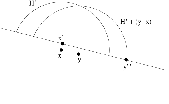
Figure 1: Illustration for proof of Lemma 3.2. The segment $H^{\prime}$ is centred on $x$.

Since $\,{\rm dist}(y,\partial A)\geq\,{\rm dist}(x,\partial A)$, using (3.3) we have

$$h(y)\geq\phi(\pi(y))+h(x)\geq h(x)-(K/9)\|\pi(y)\|^{2}.$$ (3.5)

Let $x^{\prime}$ be the point in the bounding hyperplane of $H^{\prime}$ that lies closest to $x$. Then the line segment $[x,x^{\prime}]$ is almost vertical; the angle between this line segment and the vertical is the same as that between the line segment $[x,y]$ and the horizontal. Therefore

$$\frac{h(x^{\prime})-h(x)}{\delta r}=\frac{\|\pi(y)\|}{\|y-x\|}.$$ (3.6)

Using (3.5), provided $r<1/K$ we have

$$\|y-x\|\leq\|\pi(y)\|(1+(K/9)\|\pi(y)\|)\leq(9/8)\|\pi(y)\|,$$

so we obtain from (3.6) that

$$h(x^{\prime})-h(x)\geq(8/9)\delta r.$$

Now letting $y^{\prime\prime}$ be the point in $H^{\prime}+(y-x)$ with lowest $d$-coordinate, we have that $y^{\prime\prime}=x^{\prime}+a(y-x)$ with $a=1+(1-\delta^{2})^{1/2}r/\|y-x\|$ (note $H^{\prime}$ is not quite a half-ball). Hence

$$h(x^{\prime})-h(y^{\prime\prime})\leq\left(\frac{3r}{\|y-x\|}\right)(h(x)-h(y))\leq Kr^{2},$$

where the last inequality came from (3.5). Hence, provided $r<\delta/(3K)$,

$$h(y^{\prime\prime})=h(x^{\prime})-(h(x^{\prime})-h(y^{\prime\prime}))\geq h(x)+(8/9)\delta r-Kr^{2}\geq\delta r/2.$$

On the other hand, for all $z\in H^{\prime}+(y-x)$ we have $\|\pi(z)\|\leq 2r$, so that $\phi(\pi(z))\leq Kr^{2}$ by (3.3). Provided $r<\delta/(2K)$ we therefore have $\phi(\pi(z))\leq\delta r/2\leq h(z)$ and hence $z\in A$. Therefore $H^{\prime}+(y-x)\subset A$. Also $H^{\prime}$ contains a ball of radius $r/4$ since $\delta<1/2$. Therefore using Lemma 3.1, we have

$$|A\cap B_{r}(y)\setminus B_{r}(x)|\geq|(H^{+}+(y-x))\setminus H^{+}|\geq 8^{-d}\theta_{d-1}r^{d-1}\|y-x\|,~{}~{}{\rm if~{}}h(y)<h(x).$$

Combined with (3.4) this yields (3.2), completing the proof of Part (ii).     

3.2 Integral asymptotics

For $a\in[0,1]$, let $h(a):=|B_{1}(o)\cap([0,a]\times\mathbb{R}^{d-1})|$ (we suppress the dependence of $h(a)$ on on the dimension $d$ from the notation). The following lemma is very useful for estimating the integral of $\mathbb{P}[x\in V_{t,r,k}]$ (where $V_{t,r,k}$ was defined at (2.11)) over a region near the boundary of $A$.

Lemma 3.3.

Let $\ell,j\in\mathbb{Z}_{+}:=\mathbb{N}\cup\{0\}$ and let $\alpha_{0}>0$, $\varepsilon\in(0,1)$. Then as $s\to\infty$,

$$\theta_{d-1}\int_{0}^{1}e^{-sh(a)}(\alpha_{0}+h(a))^{\ell}da=\alpha_{0}^{\ell}s^{-1}+\ell\alpha_{0}^{\ell-1}s^{-2}+O(s^{\varepsilon-3}).$$ (3.7)

Also

$$\theta_{d-1}\int_{0}^{1}e^{-sh(a)}\left(\alpha_{0}+h(a)\right)^{j}\left(1+\frac{j}{s\left(\alpha_{0}+h(a)\right)}\right)da=\alpha_{0}^{j}s^{-1}+2j\alpha_{0}^{j-1}s^{-2}+O(s^{\varepsilon-3}).$$ (3.8)

Proof.

Note first, for $0<x<1$, that

$$h(x) =\theta_{d-1}\int_{0}^{x}(1-y^{2})^{(d-1)/2}dy=\theta_{d-1}\int_{0}^{x}\left(1+O(y^{2})\right)dy$$

$$=\theta_{d-1}x+O(x^{3})~{}~{}~{}{\rm as}~{}x\downarrow 0.$$

Thus, setting $w=\theta_{d-1}sa$, we have $h(a)=w/s+O((w/s)^{3})$, and $e^{-sh(a)}=e^{-w}(1+O(w^{3}/s^{2}))$. Given $i\in\mathbb{Z}_{+}$, let $\delta=\varepsilon/(4+i)$. Then

$$\theta_{d-1}\int_{0}^{s^{\delta-1}}e^{-sh(a)}h(a)^{i}da =\int_{0}^{\theta_{d-1}s^{\delta}}e^{-w}\Big{(}1+O\big{(}\frac{w^{3}}{s^{2}}\big{)}\Big{)}\Big{(}\frac{w^{i}}{s^{i+1}}\Big{)}\Big{(}1+O\big{(}\frac{w^{2}}{s^{2}}\big{)}\Big{)}^{i}dw$$

$$=s^{-i-1}\Big{(}i!-\int_{\theta_{d-1}s^{\delta}}^{\infty}e^{-w}dw\Big{)}+O(s^{-i-3}s^{\delta(4+i)})$$

$$=i!s^{-i-1}+O(s^{\varepsilon-i-3}).$$

Also $\int_{s^{\delta-1}}^{1}e^{-sh(a)}h(a)^{i}da$ is $O(e^{-(\theta_{d-1}/2)s^{\delta}})$ since $(\theta_{d-1}/2)s^{\delta-1}\leq h(a)\leq\theta_{d}/2$ for $a$ in this range. Therefore by binomial expansion, for $\ell\in\mathbb{Z}_{+}$ we have (3.7). Applying (3.7) with $\ell=j$ and (if $j>0$) also with $\ell=j-1$ gives us (3.8).     

4 Probability approximations

In this section we assume $k\in\mathbb{N}$ is fixed and $(r_{t})_{t>0}$ is given and satisfies $tr_{t}^{d}=\Theta(\log t)$ as $t\to\infty$. With $V_{t,r,k}$ defined at (2.11), for $x,y\in A$ we define

$$p_{t}(x):=\mathbb{P}[x\in V_{t,r_{t},k}];~{}~{}~{}~{}~{}\pi_{t}(x,y):=\mathbb{P}[\{x,y\}\subset V_{t,r_{t},k}].$$ (4.1)

Since $k$ is fixed we are suppressing the dependence on $k$ in this notation. For Borel $B\subset A$ with $|B|>0$, we define

$$\gamma_{t}(B):=(t/|B|)\mathbb{E}\,[|V_{t,r_{t},k}\cap B|]=(t/|B|)\int_{B}p_{t}(x)dx,$$ (4.2)

where the second identity in (4.2) comes from Fubini’s theorem.

In Lemma 4.1 below we approximate $\mathbb{P}[R^{\prime}_{t,\tau t,k}(B)\leq r_{t}]$ using Poisson approximation (by the Chen-Stein method) for the number of $Y$-points lying in the region $V_{t,r_{t},k}$. Then in Lemma 4.2 we approximate $\mathbb{P}[R_{n,m,k}(B)\leq r_{n}]$ by a suitable coupling of Poisson and binomial point processes.

Lemma 4.1 (Poisson approximation).

Suppose A1, A2 or A3 holds. Assume that $\gamma_{t}(B)=O(1)$ as $t\to\infty$. Let $\tau\in(0,\infty)$. Let $\varepsilon>0$. Then

$$\sup_{\tau\in(\varepsilon,1/\varepsilon)}|\mathbb{P}[R^{\prime}_{t,\tau t,k}(B)\leq r_{t}]-e^{-\tau\gamma_{t}(B)}|=O((\log t)^{1-d}).$$

Proof.

Let $W_{t}:=\sum_{y\in{\cal Q}_{\tau t}}{\bf 1}\{{\cal P}_{t}(B_{r_{t}}(y))<k\}.$ Then $\mathbb{P}[R^{\prime}_{t,\tau t,k}(B)\leq r_{t}]=\mathbb{P}[W_{t}=0]$.

Let $d_{{\rm TV}}$ denote total variation distance (see e.g. [9]). Then $|\mathbb{P}[W_{t}=0]-e^{\tau\gamma_{t}(B)}|\leq d_{{\rm TV}}(W_{t},Z_{\tau\gamma_{t}(B)})$. Hence, by a similar argument to [9, Theorem 6.7],

$$|\mathbb{P}[W_{t}=0]-e^{\tau\gamma_{t}(B)}|\leq 3(I_{1}(t)+I_{2}(t)),$$

where, with $p_{t}(x)$ and $\pi_{t}(x,y)$ defined at (4.1), we set

$$I_{1}(t) :=\tau^{2}(t/|B|)^{2}\int_{B}\int_{B(x,3r_{t})\cap B}p_{t}(x)p_{t}(y)dydx;$$ (4.3)

$$I_{2}(t) :=\tau^{2}(t/|B|)^{2}\int_{B}\int_{B(x,3r_{t})\cap B}\pi_{t}(x,y)dydx.$$ (4.4)

Define the Borel measure $\nu$ on $\mathbb{R}^{d}$ by

$$\nu(\cdot):=\lambda_{d}(\cdot\cap A)/|A|,$$ (4.5)

where $\lambda_{d}$ denotes $d$-dimensional Lebesgue measure. Under any of A1, A2 or A3 (using Lemma 3.2 in the case of A1), we can and do choose $\delta>0$ such that for all $y\in B$ and all $r\in(0,1]$ we have $\nu(B_{r}(y))\geq 2\delta r^{d}$. Hence, for all large enough $t$ and all $y\in B$ we have

$$p_{t}(y)=\sum_{j=0}^{k-1}((t\nu(B_{r_{t}}(x)))^{j}/j!)e^{-t\nu(B_{r}(x))}\leq\exp(-\delta tr_{t}^{d}).$$

Since $(t/|B|)\int_{B}p_{t}(x)dx=\gamma_{t}(B)\to\gamma$, we have

$$I_{1}(t)\leq\tau^{2}|B|^{-1}(t\theta_{d}(3r_{t})^{d})e^{-\delta tr_{t}^{d}}(t/|B|)\int_{B}p_{t}(x)dx=O(e^{-(\delta/2)tr_{t}^{d}}).$$ (4.6)

Now consider $I_{2}(t)$. For $x,y\in A$ let us write $x\prec y$ if $x$ is closer than $y$ to $\partial A$ (in the Euclidean norm), or if $x$ and $y$ are the same distance from $\partial A$ but $x$ precedes $y$ lexicographically. Since $\pi_{t}(x,y){\bf 1}\{\|y-x\|\leq 3r_{t}\}$ is symmetric in $x$ and $y$, we have

$$\int_{B}\int_{B(x,3r_{t})\cap B}\pi_{t}(x,y)dydx=2\int_{B}\int_{\{y\in B\cap B(x,3r_{t}):x\prec y\}}\pi_{t}(x,y)dydx.$$ (4.7)

By the independence properties of the Poisson process we have

$$\pi_{t}(x,y)\leq p_{t}(x)\sum_{m=0}^{k-1}q_{t,m}(y,x),$$

where we set $q_{t,m}(y,x):=\mathbb{P}[{\cal P}_{t}(B_{r_{t}}(y)\setminus B_{r_{t}}(x))=m].$

Suppose Assumption A1 or Assumption A3 applies. Set $\kappa_{d}:=8^{-d}\theta_{d-1}$. By Lemma 3.2 (ii), for all large enough $t$ and all $x,y\in B$ with $x\prec y$ and $\|y-x\|\leq 2r_{t}$, we have $\nu(B_{r_{t}}(y)\setminus B_{r_{t}}(x))\geq\kappa_{d}f_{0}r_{t}^{d-1}\|y-x\|$. Moreover by Fubini’s theorem $\nu(B_{r_{t}}(y)\setminus B_{r_{t}}(x))\leq\theta_{d-1}f_{0}r_{t}^{d-1}\|y-x\|$. Hence for all $m\leq k-1$,

$$q_{t,m}(y,x)\leq(tf_{0}\theta_{d-1}r_{t}^{d-1}\|y-x\|)^{m}\exp(-\kappa_{d}f_{0}tr_{t}^{d-1}\|y-x\|).$$

Hence, setting $B_{x}:=\{y\in B:x\prec y\}$ we have that

$$t\int_{B_{x}\cap B(x,3r_{t})}q_{t,m}(y,x) \leq f_{0}^{m}\theta_{d-1}^{m}t\int_{B(o,3r_{t})}(tr_{t}^{d-1}\|y\|)^{m}\exp(-\kappa_{d}f_{0}tr_{t}^{d-1}\|y\|)dy$$

$$=f_{0}^{m}\theta_{d-1}^{m}t(tr_{t}^{d-1})^{-d}\int_{B(o,3tr_{t}^{d})}\|z\|^{m}\exp(-\kappa_{d}f_{0}\|z\|)dz$$

$$\leq c(tr_{t}^{d})^{1-d},$$

for some constant $c$ depending only on $d,f_{0}$ and $k$. Therefore

$$t^{2}\int_{B}\int_{B(x,3r_{t})\cap B}\pi_{t}(x,y)dydx\leq 2\left(t\int_{B}p_{t}(x)dx\right)ck(tr_{t}^{d})^{1-d}.$$

Since the expression in brackets on the right is $O(1)$ by assumption, we thus have $I_{2}(t)=O((tr_{t}^{d})^{1-d})=O((\log t)^{1-d})$.

Now suppose we assume instead that Assumption A2 applies. First we examine the situation where $x$ is not too close to the corners of $A$. Suppose that $\,{\rm dist}(x,\Phi_{0}(A))>Kr_{t}$, where $K$ is made explicit later. We can assume that the corner of $A$ closest to $x$ is formed by edges $e,e^{\prime}$ meeting at the origin with angle $\alpha\in(0,2\pi)\setminus\{\pi\}$. We claim that, provided $K>4+8/|\sin\alpha|$, the disk $B(x,4r_{t})$ intersects at most one of the two edges. Indeed, if it intersects both edges, then taking $w\in B(x,4r_{t})\cap e,w^{\prime}\in B(x,4r_{t})\cap e^{\prime}$ we have $\|w-w^{\prime}\|\leq 8r_{t}$; hence $\,{\rm dist}(w,e^{\prime})\leq 8r_{t}$. Then, $\|w\|=\,{\rm dist}(w,e^{\prime})/|\sin\alpha|\leq 8r_{t}/|\sin\alpha|$. However, $\|w\|\geq(K-4)r_{t}$ by the triangle inequality, so we arrive at a contradiction. Also, for $t$ sufficiently large, non-overlapping edges of $A$ are distant more than $8r_{t}$ from each other. We have thus shown that if we take $K=5+(8/\min_{i}|\sin\alpha_{i}|)$, where $\{\alpha_{i}\}$ are the angles of the corners of $A$, then for large $t$, no ball of radius $4r_{t}$ distant at least $Kr_{t}$ from the corners of $A$ can intersect two or more edges of $A$ at the same time.

We have $B(x,r_{t})\cup B(y,r_{t})\subset B(x,4r_{t})$. Hence, the argument leading to Lemma 3.2-(ii) shows that $\nu(B(y,r_{t})\setminus B(x,r_{t}))\geq\theta_{d-1}8^{-d}f_{0}\|x-y\|r_{t}$. Using this, we can estimate the contribution to the double integral on the right side of (4.7) in the same way as we did under assumption A1.

Suppose instead that $x$ is close to a corner of $A$ and $\|x-y\|\leq 3r_{t}$. The contribution to the double integral on the right side of (4.7) from such pairs $(x,y)$ is at most $c^{\prime\prime}t^{2}r_{t}^{4}\exp(-\delta_{1}tr_{t}^{2})$ where $c^{\prime\prime}$ depends only on $K$ and $\delta_{1}>0$ depends only on $A$. Therefore this contribution tends to zero, and the proof is now complete.     

Lemma 4.2 (De-Poissonization).

Suppose A1, A2 or A3 holds. Let $m(n)$ be such that $m(n)=\Theta(n)$ as $n\to\infty$. Assume $\gamma_{n}(B)=O(1)$ as $n\to\infty$. Then

$$|\mathbb{P}[R_{n,m(n),k}(B)\leq r_{n}]-e^{-(m(n)/n)\gamma_{n}(B)}|=O((\log n)^{1-d}).$$

Proof.

Write $m$ for $m(n)$. Set $n^{+}:=n+n^{3/4}$, $n^{-}:=n-n^{3/4}$ and $m^{+}:=m+m^{3/4},m^{-}:=m-m^{3/4}$. Set

$$W:=\sum_{y\in{\cal Y}_{m}}{\bf 1}\{\mathcal{X}_{n}(B_{r_{n}}(y))<k\};~{}~{}~{}W^{\prime}:=\sum_{y\in{\cal Q}_{m^{-},B}}{\bf 1}\{{\cal P}_{n^{+}}(B_{r_{n}}(y))<k\}.$$

Set $\gamma^{\prime}_{n}:=(n^{-}/|B|)\mathbb{E}\,[|V_{{n^{+}},r_{n},k}\cap B|]$, where $V_{n,r,k}$ was defined at (2.11). Then, with the measure $\nu$ defined at (4.5),

$$\gamma^{\prime}_{n} =\frac{n^{-}}{|B|}\int_{B}\left(e^{-n\nu(B(x,r_{n}))-n^{3/4}\nu(B(x,r_{n}))}\sum_{j=0}^{k-1}(n(1+n^{-1/4}))^{j}\nu(B(x,r_{n}))^{j}/j!\right)dx$$

$$=\gamma_{n}(B)(1+O((\log n)^{1/d}n^{-1/4})).$$ (4.8)

By Lemma 4.1, $|\mathbb{P}[R^{\prime}_{n^{+},m^{-},k}(B)\leq r_{n}]-e^{-(m^{-}/n^{+})\gamma^{\prime}_{n}}|=O((\log n)^{1-d})$, and hence by (4.8), $|\mathbb{P}[R^{\prime}_{n^{+},m^{-},k}(B)\leq r_{n}]-e^{-(m^{-}/n^{+})\gamma_{n}(B)}|=O((\log n)^{1-d})$. Note also that $|(m/n)-(m^{-}/n^{+})|=O(n^{-1/4})$ so that $|e^{-(m/n)\gamma_{n}(B)}-e^{-(m^{-}/n^{+})\gamma_{n}(B)}|=O(n^{-1/4})$. Also

$$|\mathbb{P}[R_{n,m(n),k}(B)\leq r_{n}]-\mathbb{P}[R^{\prime}_{n^{+},m^{-},k}(B)\leq r_{n}]|\leq\mathbb{P}[W\neq W^{\prime}].$$

We have the event inclusion $\{W\neq W^{\prime}\}\subset E_{1}\cup E_{2}\cup E_{3}$, where, recalling the definition of $(Z_{t})_{t\geq 0}$ in Section 1, we define the events

$$E_{1} :=\{Z_{m^{-}}\leq m\leq Z_{m^{+}}\}^{c}\cup\{Z^{\prime}_{n^{-}}\leq n\leq Z^{\prime}_{n^{+}}\}^{c};$$

$$E_{2} :=\{\exists y\in{\cal Q}_{m^{-}}:{\cal P}_{n^{-}}(B(y,r_{n}))<k,({\cal P}_{n^{+}}\setminus{\cal P}_{n^{-}})(B(y,r_{n}))\neq 0\};$$

$$E_{3} :=\{\exists y\in{\cal Q}_{m^{+}}\setminus{\cal Q}_{m^{-}}:{\cal P}_{n^{-}}(B(y,r_{n}))<k\}.$$

By Chebyshev’s inequality $\mathbb{P}[E_{1}]=O(n^{-1/2})$. Also by a similar calculation to (4.8), $(n/|B|)\mathbb{E}\,[|V_{n^{-},r_{n},k}\cap B|]=\gamma_{n}(B)(1+O((\log n)n^{-1/4}))$, and

$$\mathbb{P}[E_{2}]\leq\mathbb{E}\,[|V_{n^{-},r_{n},k}\cap B|/|B|]m^{-}(2n^{3/4})f_{0}\theta_{d}r_{n}^{d}=O(n^{-1/4}\log n).$$

Similarly $\mathbb{P}[E_{3}]=2m^{3/4}\mathbb{E}\,[|V_{n^{-},r_{n},k}\cap B|/|B|]=O(n^{-1/4})$. Combining these estimates gives the result.     

5 Proof of Theorems

5.1 Proof of Theorem 2.1

Recall the definition of $\gamma_{t}(B)$ at (4.2). For each theorem, we need to find $(r_{t})_{t\geq 0}$ such that $\gamma_{t}(B)$ converges as $t\to\infty$; we can then apply Lemmas 4.1 and 4.2. We are ready to do this for Theorem 2.1 without further ado. Recall that $f_{0}:=1/|A|$.

Proof of Theorem 2.1.

Fix $k\in\mathbb{N}$, $\beta\in\mathbb{R}$. For all $t>0$ define $r_{t}\in[0,\infty)$ by

$$tf_{0}\theta_{d}r_{t}^{d}=\max(\log t+(k-1)\log\log t+\beta,0).$$

Set $j=k-1$. Since we assume here that $\overline{B}\subset A^{o}$, as $t\to\infty$ we have uniformly over $x\in B$ that

$$\mathbb{P}[x\in V_{t,r_{t},k}] =e^{-tf_{0}\theta_{d}r_{t}^{d}}((tf_{0}\theta_{d}r_{t}^{d})^{j}/j!)(1+j(f_{0}\theta_{d}r_{t}^{d})^{-1}+O((\log t)^{-2})),$$

$$=(1/j!)t^{-1}(\log t)^{-j}e^{-\beta}(\log t+j\log\log t+\beta)^{j}$$

$$~{}~{}~{}~{}~{}~{}~{}~{}~{}~{}~{}~{}~{}~{}\times(1+j(\log t+j\log\log t+\beta)^{-1}+O((\log t)^{-2}))$$

$$=\frac{e^{-\beta}}{j!t}\Big{(}1+\frac{j\log\log t+\beta}{\log t}\Big{)}^{j}\Big{(}1+j(\log t)^{-1}\Big{(}1+\frac{j\log\log t+\beta}{\log t}\Big{)}^{-1}$$

$$~{}~{}~{}~{}~{}~{}~{}~{}~{}~{}~{}~{}~{}~{}~{}~{}~{}~{}~{}~{}~{}~{}~{}~{}~{}~{}~{}~{}~{}~{}~{}~{}~{}~{}~{}~{}~{}~{}~{}~{}~{}~{}~{}~{}~{}~{}~{}~{}~{}~{}~{}~{}~{}~{}~{}~{}~{}~{}~{}~{}~{}+O\big{(}(\log t)^{-2}\big{)}\Big{)},$$

where the $O(\cdot)$ term is zero for $k=1$ or $k=2$. Using (4.2), we obtain by standard power series expansion that as $t\to\infty$ we have

$$\gamma_{t}(B) =\frac{e^{-\beta}}{j!}\Big{(}1+\frac{j^{2}\log\log t}{\log t}+\frac{j(1+\beta)}{\log t}+O\big{(}\big{(}\frac{\log\log t}{\log t}\big{)}^{2}\big{)}\Big{)}.$$ (5.1)

Hence by Lemma 4.1, given $\tau\in(0,\infty)$ as $t\to\infty$ we have

$$\mathbb{P}[R^{\prime}_{t,\tau t,k}(B)\leq r_{t}]=\exp\Big{(}-\frac{\tau e^{-\beta}}{j!}\Big{(}1+\frac{j^{2}\log\log t}{\log t}+\frac{j(1+\beta)}{\log t}+O\big{(}\big{(}\frac{\log\log t}{\log t}\big{)}^{2}\big{)}\Big{)}\Big{)}$$

$$~{}~{}~{}~{}~{}~{}~{}~{}~{}~{}~{}~{}~{}~{}~{}~{}~{}~{}~{}~{}~{}~{}~{}~{}~{}~{}~{}~{}~{}~{}~{}~{}~{}~{}~{}~{}~{}~{}~{}~{}~{}~{}~{}~{}~{}~{}~{}~{}~{}~{}~{}~{}~{}~{}~{}~{}~{}~{}~{}~{}~{}~{}~{}~{}~{}~{}~{}~{}~{}+O((\log t)^{1-d})$$

$$=\begin{cases}e^{-\tau e^{-\beta}/j!}\left(\exp\big{(}-\frac{\tau e^{-\beta}j^{2}\log\log t}{j!\log t}\big{)}+O\big{(}(\log t)^{-1}\big{)}\right)~{}~{}~{}~{}~{}~{}~{}~{}~{}~{}~{}~{}~{}~{}~{}~{}~{}~{}~{}~{}{\rm if}~{}d=2\\ e^{-\tau e^{-\beta}/j!}\left(\exp\big{(}-\frac{\tau e^{-\beta}j^{2}\log\log t}{j!\log t}-\frac{\tau e^{-\beta}j(1+\beta)}{j!\log t}\big{)}+O\big{(}\big{(}\frac{\log\log t}{\log t}\big{)}^{2}\big{)}\right)~{}~{}~{}{\rm if}~{}d\geq 3,\end{cases}$$ (5.2)

yielding (2.3). Similarly, given also $m:\mathbb{N}\to\mathbb{N}$ satisfying $\tau_{n}:=m(n)/n\to\tau$ as $n\to\infty$, by Lemma 4.2 and (5.1) we have as $n\to\infty$ that

$$\mathbb{P}[R_{n,m(n),k}(B)\leq r_{n}]$$

$$=\begin{cases}e^{-\tau_{n}e^{-\beta}/j!}\exp\Big{(}-\frac{\tau_{n}e^{-\beta}j^{2}\log\log n}{j!\log n}\Big{)}+O\big{(}(\log n)^{-1}\big{)}~{}~{}~{}~{}~{}~{}~{}~{}~{}~{}~{}~{}~{}~{}~{}~{}~{}~{}~{}~{}~{}{\rm if}~{}d=2\\ e^{-\tau_{n}e^{-\beta}/j!}\exp\Big{(}-\frac{\tau_{n}e^{-\beta}j^{2}\log\log n}{j!\log n}-\frac{\tau_{n}e^{-\beta}j(1+\beta)}{j!\log n}\Big{)}+O\big{(}\big{(}\frac{\log\log n}{\log n}\big{)}^{2}\big{)}~{}~{}~{}{\rm if}~{}d\geq 3,\end{cases}$$ (5.3)

and (2.2) follows.     

Under assumption A1 or A2 (with $B=A$), it takes more work than in the preceding proof to determine $r_{t}$ such that $\gamma_{t}(A)$ tends to a finite limit. The right choice turns out to be as follows. Let $\beta\in\mathbb{R}$ and let $r_{t}=r_{t}(\beta)\geq 0$ be given by

$$f_{0}t\theta_{d}r_{t}^{d}=\max\Big{(}\big{(}2-2/d\big{)}\log t+\big{(}2k-4+2/d\big{)}{\bf 1}_{\{d\geq 3\text{ or }k\geq 2\}}\log\log t+\beta,0\Big{)},$$ (5.4)

where $f_{0}:=|A|^{-1}$. We show in the next two subsections that this choice of $r_{t}$ works.

5.2 Convergence of $t\mathbb{E}[|V_{t,r_{t},k}|]$ for $d=2$

We now demonstrate convergence of $t\mathbb{E}\,[|V_{t,r_{t},k}|]$ when $d=2$.

Proposition 5.1 (Convergence of the expectation when $d=2$).

Suppose $d=2$ and A1 or A2 applies. Fix $\beta\in\mathbb{R}$, and let $r_{t},V_{t,r,k}$ be as given in (5.4) and (2.11). Then as $t\to\infty$,

$$t\mathbb{E}[|V_{t,r_{t},k}|]=\begin{cases}|A|e^{-\beta}+|\partial A|e^{-\beta/2}\frac{\sqrt{\pi/f_{0}}}{2}(\frac{1}{\sqrt{\log t}}+O((\log t)^{-3/2}))&\mbox{ if }k=1\\ |A|e^{-\beta}+|\partial A|e^{-\beta/2}\frac{\sqrt{\pi/f_{0}}}{4}\Big{(}1+\frac{\log\log t}{2\log t}\Big{)}+\frac{|A|e^{-\beta}\log\log t}{\log t}\\ ~{}~{}~{}~{}~{}~{}~{}~{}~{}~{}~{}~{}~{}~{}~{}~{}~{}~{}~{}~{}~{}~{}~{}~{}~{}~{}~{}~{}~{}~{}~{}~{}~{}~{}~{}~{}~{}~{}~{}+O((\log t)^{-1}))&\mbox{ if }k=2\\ |\partial A|e^{-\beta/2}\frac{\sqrt{\pi/f_{0}}}{(k-1)!2^{k}}\left(1+\frac{(2k-3)^{2}\log\log t}{2\log t}\right)+O\big{(}\frac{1}{\log t}\big{)}&\mbox{ if }k\geq 3\end{cases}$$ (5.5)

Proof.

Recall $p_{t}(x)$ at (4.1). By Fubini’s theorem, as at (4.2), we have

$$\mathbb{E}[|V_{t,r_{t},k}|]=\int_{A}p_{t}(x)dx.$$ (5.6)

Case 1: $A$ has a $C^{2}$ boundary and $\overline{A^{o}}=A$. To estimate the integral in the optimal way, we decompose $A$ into several pieces with regards to a certain polygonal approximation of the set $A$.

Step 1: polygonal approximation of $A$. Let $\alpha=3/8$ (in fact any $\alpha\in(1/4,1/2)$ would work). Since we assume $A$ is compact and has a $C^{2}$ boundary, its boundary $\partial A$ consists of a finite number of Jordan curves (if $A$ is simply-connected, that number is 1).

Given $t$, for each component $\gamma$ of $\partial A$ we draw points iteratively from $\gamma$ in such a way that every two consecutive points are at distance $t^{-\alpha}$ until we make a tour. If the distance between the first point and the last point in the tour is less than $t^{-\alpha}$, we remove the last point. Then we draw segments according to the order of these points. All segments except the last one are of length $t^{-\alpha}$. By triangle inequality, the length of the last segment is in the range $[t^{-\alpha},2t^{-\alpha}]$. Let $A_{t}$ denote the set that is bounded by the union of these polygons (one for each component of $\partial A$). We claim that this set is a good approximation of $A$ in the sense that

$$\,{\rm dist}(\partial A_{t},\partial A)=O(t^{-2\alpha})~{}~{}~{}{\rm as}~{}t\to\infty,$$ (5.7)

where $\,{\rm dist}$ denotes the Euclidean distance between compact sets. Indeed, there exist a finite number of open intervals $I_{i}$ and $C^{2}$ functions $\phi_{i}$ defined on $I_{i}$ such that $\partial A$ is the union of the (possibly rotated and translated) graphs of these functions. Let $c$ be the maximum over $i$ of the uniform norm of $(\phi_{i})^{\prime\prime}$.

Each segment of $\partial A_{t}$ is of the form $\{(u,f(u)):u\in[a,b]\}$, with $[a,b]\subset I_{i}$ for some $i$, with $(a,\phi_{i}(a))$ and $(b,\phi_{i}(b))$ consecutive vertices of one of the polygons making up $\partial A_{t}$ (to ease notation we assume no rotation of $I_{i}$ is needed) and with the graph of $f$ interpolating linearly from $(a,\phi_{i}(a))$ to $(b,\phi_{i}(b))$.

Using the Mean Value theorem repeatedly and the assumption that $\phi_{i}\in C^{2}$, one has

$$\max_{u\in[a,b]}|\phi_{i}(u)-f(u)| =\max_{u\in[a,b]}|\phi_{i}(u)-\phi_{i}(a)-\phi^{\prime}_{i}(z)(u-a)|$$

$$=\max_{u\in[a,b]}|(\phi^{\prime}_{i}(v)-\phi^{\prime}_{i}(z))(u-a)|\leq c|b-a|^{2}$$

where $z\in[a,b]$ is such that $\phi_{i}^{\prime}(z)$ is the slope of the segment $[(a,\phi_{i}(a)),(b,\phi_{i}(b))]$ whose existence is guaranteed by the Mean Value theorem, and $v\in[a,u]$ is such that $\phi_{i}^{\prime}(v)$ is the slope of the segment $[(a,\phi_{i}(a)),(u,\phi_{i}(u))]$. Hence $\max_{i}\sup_{u\in I_{i}}|f(u)-\phi_{i}(u)|=O(t^{-2\alpha})$, and therefore any point in $\partial A_{n}$ is distant at most $O(t^{-2\alpha})$ from a point in $\partial A$, and vice versa. This justifies the claim (5.7).

Notice that our choice of $\alpha$ implies that $t^{-2\alpha}\ll r_{t}(\beta)\ll t^{-\alpha}$, where $a_{t}\ll b_{t}$ means $a_{t}/b_{t}\to 0$, and $r_{t}(\beta)$ was defined at (5.4). Thus by (5.7), $\partial A_{t}$ is very close to $\partial A$ compared to $r_{t}$.

We shall also need shrunken versions of $A_{t}$ defined by

$$A_{t}^{1} =\{x\in A_{t}:\,{\rm dist}(x,\partial A_{t})\geq r_{t}(\beta)+Kt^{-2\alpha}\};$$ (5.8)

$$A_{t}^{2} =\{x\in A_{t}:\,{\rm dist}(x,\partial A_{t})\geq Kt^{-2\alpha}\},$$ (5.9)

with $K$ chosen so that $A_{t}^{2}$ (and hence also $A_{t}^{1}$) is a subset of $A$ for large $t$, which can be done by (5.7). Moreover, for suitably chosen $K$, we have $B(y,r_{t}(\beta))\subset A$ for any $y\in A_{t}^{1}$. We refer to $A_{t}^{1}$ as the bulk, $\mathsf{Mo}_{t}:=A_{t}^{2}\setminus A_{t}^{1}$ as the moat, and $\mathsf{Rai}_{t}:=A\setminus A_{t}^{2}$ the railing. As such, $A$ is partitioned into the bulk, the moat and the railing.

Step 2: contribution to (5.6) from the bulk. By (4.1), for $x\in A_{t}^{1}$ we have

$$p_{t}(x)=\frac{1}{(k-1)!}e^{-tf_{0}\pi r_{t}^{2}}(tf_{0}\pi r_{t}^{2})^{k-1}\Big{(}1+\frac{k-1}{tf_{0}\pi r_{t}^{2}}+O(\frac{1}{(tr_{t}^{2})^{2}})\Big{)},$$

where the big O term is $0$ when $k=1$ or $k=2$. Also by (5.4), for $t$ large we have $e^{-tf_{0}\pi r_{t}^{2}}=e^{-\beta}t^{-1}(\log t)^{(3-2k){\bf 1}_{\{k\geq 2\}}}$. Hence for $k\geq 2$ and $x\in A_{t}^{1}$ we have

$$p_{t}(x)=(t^{-1}e^{-\beta}/(k-1)!)(\log t)^{3-2k}(\log t+(2k-3)\log\log t+\beta)^{k-1}$$

$$\times(1+(k-1)(\log t)^{-1}(1+O((\log\log t)/\log t))),$$

while if $k=1$ and $x\in A_{t}^{1}$ then $p_{t}(x)=e^{-\beta}t^{-1}$. Hence, since $|A_{t}^{1}|=|A_{t}|+O(r_{t})$,

$$\int_{A^{1}_{t}}p_{t}(x)tdx=\begin{cases}e^{-\beta}|A|(1+O(r_{t}))&\mbox{ if }k=1,\\ e^{-\beta}|A|\big{(}1+\frac{\log\log t}{\log t}+\frac{\beta+1}{\log t}+O(\frac{\log\log t}{(\log t)^{2}})\big{)}&\mbox{ if }k=2,\\ \frac{e^{-\beta}}{(k-1)!(\log t)^{k-2}}+O(\frac{\log\log t}{(\log t)^{k-1}})&\mbox{ if }k\geq 3.\end{cases}$$ (5.10)

Step 3: contribution from the moat. By construction, the moat is piecewise linear with width $r_{t}$ and the number of pieces, denoted $m(t)$, is $O(t^{\alpha})$. We can decompose as follows:

$$\mathsf{Mo}_{t}=\bigcup_{i=1}^{m(t)}\mathsf{Rec}_{t,i}\cup\bigcup_{i=1}^{m(t)}\mathsf{Cor}_{t,i}$$ (5.11)

where each $\mathsf{Rec}_{t,i}$ corresponds to the maximal rectangle fitted into each linear piece of the moat that is at distance $r_{t}$ from the vertices of $A_{t}^{2}$, and $\mathsf{Cor}_{t,i},1\leq i\leq m(t)$ are the ‘corner pieces’ given by the connected components of $\mathsf{Mo}_{t}\setminus\cup_{i=1}^{m(t)}\mathsf{Rec}_{t,i}$ (with $\mathsf{Cor}_{t,i}$ adjacent to $\mathsf{Rec}_{t,i}$ in a counter-clockwise direction for each $i$).

For $x\in\sf{Rec}_{t,i}$ let $a(x)$ denote the distance from $x$ to the side of $\sf{Rec}_{t,i}$ that is adjacent to the railing (we call this the ‘lower’ side of $\sf{Rec}_{t,i}$). As in Section 3.2, set $h(a):=|B_{1}(o)\cap([0,a]\times\mathbb{R})|$, $a>0$. We claim, for all large enough $t$, all $i\leq m(t)$ and all $x\in\mathsf{Rec}_{t,i}$ that

$$|B_{r_{t}}(x)\cap A|\geq r_{t}^{2}((\pi/2)+h(a(x)/r_{t})).$$

Indeed, by the $C^{2}$ boundary assumption and a compactness argument there exists $\delta>0$ such that after a rotation we may assume that the part of $\partial A$ within distance $\delta$ of $\mathsf{Rec}_{t,i}$ is the graph of a function with slope in the range $[-\tan\pi/9,\tan\pi/9]$ and hence the angle between the lower side of $\sf{Rec}_{t,i}$ and that of that $\sf{Rec}_{i-1}$ is between $3\pi/4$ and $5\pi/4$, and likewise for $\sf{Rec}_{t,i+1}$. Therefore $\sf{Rec}_{t,i}$ does not lie within distance $r_{t}$ of any part of $\partial A$, other than the part approximated by the lower boundary of $\sf{Rec}_{t,i}$, justifying the lower bound.

On the other hand, using (5.7) and the fact that $h^{\prime}(a)\leq\theta_{d-1}$ for every $a\in(0,1)$, we have

$$|B_{r_{t}}(x)\cap A|\leq r_{t}^{2}\big{(}\pi/2+h(a(x)/r_{t})+O(r_{t}^{-1}t^{-2\alpha})\big{)}.$$

By the preceding claims and a simple coupling, as well as (4.1), for all large enough $n$, all $i\leq m(t)$ and all $x\in\mathsf{Rec}_{t,i}$, setting $\Lambda_{t,a}:=tf_{0}r_{t}^{2}((\pi/2)+h(a))$ we have that

$$p_{t}(x)=((k-1)!)^{-1}e^{-\Lambda_{t,a(x)/r}}\Lambda_{t,a(x)/r}^{k-1}(1+O((\log t)^{-1})),$$ (5.12)

where we have used the fact that $tr_{t}^{2}=\Theta(\log t)$ so that $t^{-2\alpha}r_{t}^{-1}=o((\log t)^{-2})$ and $\Lambda_{t,a}=\Theta(\log t)$ uniformly over $a\in[0,1]$. Hence, letting $\mathsf{BRec}_{t,i}$ denote the side of $\mathsf{Rec}_{t,i}$ approximating a portion of $\partial A$ and $|\mathsf{BRec}_{t,i}|$ its length, we have

$$t\int_{\mathsf{Rec}_{t,i}}p_{t}(x)dx= \frac{t}{(k-1)!}|\mathsf{BRec}_{t,i}|r_{t}\int_{0}^{1}e^{-\Lambda_{t,a}}\Lambda_{t,a}^{k-1}(1+O((\log t)^{-1}))da.$$ (5.13)

We claim that, with $|\partial A|$ denoting the length of $\partial A$,

$$\sum_{i=1}^{m(t)}|\mathsf{BRec}_{t,i}|=|\partial A|+O(t^{-\alpha})+O(t^{\alpha}r_{t})=|\partial A|+O((\log t)^{1/2}t^{-1/8}).$$ (5.14)

To see this, recall that each segment with endpoints on $\partial A$ in the polygonal approximation approximates a curve in $\partial A$ with the same endpoints. By compactness, we can find finite number of $C^{2}$ functions whose graphs cover $\partial A$ completely and for some $C^{2}$ function $\phi$, its graph on $[a,b]$ is that curve approximated by the segment. By the Mean Value theorem, the approximating segment has slope $\phi^{\prime}(u_{0})$ for some $u_{0}$ in $[a,b]$, and the error of approximation is

$$\left|\int_{a}^{b}\sqrt{1+\phi^{\prime}(u)^{2}}du-\int_{a}^{b}\sqrt{1+\phi^{\prime}(u_{0})^{2}}du\right|\leq c|b-a|^{2}\leq ct^{-2\alpha},$$

where $c$ depends only on the first two derivatives of the finite number of $C^{2}$ functions mentioned previously. Moreover, the length of the $i$-th segment minus that of $|\mathsf{BRec}_{t,i}|$ is at most $4r_{t}$. This, together with the fact that $m(t)=O(t^{\alpha})$, gives the claim (5.14).

Summing over $i$ in (5.13) and using (5.14) and (5.4), we have:

$$\sum_{i=1}^{m(t)}t\int_{\mathsf{Rec}_{t,i}}p_{t}(x)dx =(tr_{t}/(k-1)!)\sum_{i=1}^{m(t)}|\mathsf{BRec}_{t,i}|$$

$$~{}~{}\times\int_{0}^{1}e^{-tf_{0}r_{t}^{2}(\frac{\pi}{2}+h(a))}\left(tf_{0}r_{t}^{2}\big{(}\frac{\pi}{2}+h(a)\big{)}\right)^{k-1}\left(1+O((\log t)^{-1})\right)da$$

$$=\frac{tr_{t}}{(k-1)!}\left(|\partial A|+O(t^{\alpha}r_{t})\right)t^{-1/2}(\log t)^{-(k-3/2){\bf 1}\{k\geq 2\}}e^{-\beta/2}(tf_{0}r_{t}^{2})^{k-1}$$

$$~{}~{}\times\int_{0}^{1}e^{-tf_{0}r_{t}^{2}h(a)}\left(\frac{\pi}{2}+h(a)\right)^{k-1}\left(1+O((\log t)^{-1})\right)da.$$ (5.15)

Setting $s=tf_{0}r_{t}^{2}$, and then using (3.7) from Lemma 3.3 with $\alpha_{0}=\pi/2$ and $j=k-1$, the integral in the last line comes to

$$\int_{0}^{1}e^{-sh(a)}\left(\frac{\pi}{2}+h(a)\right)^{k-1}\left(1+O(s^{-1})\right)da=\frac{\pi^{k-1}}{2^{k}s}\left(1+O(s^{-1})\right).$$

By (5.4), $s=tf_{0}r_{t}^{2}=\pi^{-1}(\log t+(2k-3){\bf 1}_{\{k\geq 2\}}\log\log t+\beta)$ and hence for $t$ large,

$$\frac{s}{\log t}=\pi^{-1}\left(1+\frac{(2k-3){\bf 1}_{\{k\geq 2\}}\log\log t}{\log t}+O((\log t)^{-1})\right).$$

Thus we obtain from (5.15) by writing $t^{1/2}r_{t}$ in terms of $s$, that

$$\sum_{i=1}^{m(t)}t\int_{\mathsf{Rec}_{t,i}}p_{t}(x)dx=\frac{f_{0}^{-1/2}\pi^{k-1}|\partial A|}{(k-1)!2^{k}}(\log t)^{-(k-3/2){\bf 1}_{\{k\geq 2\}}}e^{-\beta/2}s^{k-3/2}(1+O(s^{-1}))$$

$$=\frac{\pi^{1/2}f_{0}^{-1/2}e^{-\beta/2}|\partial A|}{(k-1)!2^{k}}(\log t)^{-\frac{1}{2}{\bf 1}_{\{k=1\}}}\Big{(}1+\Big{(}\frac{(k-\frac{3}{2}){\bf 1}_{\{k\geq 2\}}(2k-3)\log\log t}{\log t}\Big{)}$$

$$+O\big{(}(\log t)^{-1}\big{)}\Big{)}.$$

In view of the $C^{2}$ boundary assumption and Lemma 3.2(i), given $\kappa\in(\alpha,1/2)$, for large $t$ and any $i\leq m(t)$, $x\in\mathsf{Cor}_{t,i}$, we have $p_{t}(x)\leq e^{-tf_{0}\pi r_{t}^{2}\kappa}$ and hence by (5.4), $p_{t}(x)\leq t^{-\kappa}$ (note that the coefficient of $\log\log t$ in (5.4) is positive in this case). Each $\mathsf{Cor}_{t,i}$ has area at most $\pi(2r_{t})^{2}$, and hence

$$tf_{0}\int_{\sf{Cor}_{t,i}}p_{t}(x)dx=O(tr_{t}^{2}t^{-\kappa})=O((\log t)t^{-\kappa}),$$ (5.16)

leading to a total contribution from the corners to (5.6) of $O((\log t)t^{-\kappa+\alpha})$. Hence

$$t\int_{\mathsf{Mo}_{t}}p_{t}(x)dx=\begin{cases}\frac{1}{2}|\partial A|e^{-\beta/2}\sqrt{\pi/f_{0}}((\log t)^{-1/2}+O((\log t)^{-3/2}))&k=1\\ |\partial A|e^{-\beta/2}\frac{\sqrt{\pi/f_{0}}}{(k-1)!2^{k}}\Big{(}1+\frac{(2k-3)^{2}\log\log t}{2\log t}\Big{)}+O\big{(}\frac{1}{\log t}\big{)}&k\geq 2.\end{cases}$$ (5.17)

Step 4: contribution from the railing. Using Lemma 3.2(i) as before, given $\kappa\in(1-2\alpha,1/2)$, for large $n$, we have $p_{t}(x)\leq e^{-tf_{0}\pi r_{t}^{2}\kappa}$ for $x\in\mathsf{Rai}_{t}$. By (5.7), the railing has total area at most $ct^{-2\alpha}$ for suitably chosen $c$; thus

$$t\int_{\mathsf{Rai}_{t}}p_{t}(x)dx\leq ct^{1-2\alpha}e^{-tf_{0}\pi r_{t}^{2}\kappa}=O(t^{1-2\alpha-\kappa}).$$

Combining this with (5.10) and (5.17), and using (5.6), yields (5.5) in Case 1.

Case 2: $A$ is polygonal. In this case, instead of taking a sequence of approximating polygons depending on $n$, we work directly with $A$. In this case define $A_{t}^{1}:=A^{(-r_{t})}$ (with $r_{t}=r_{t}(\beta))$, and $\mathsf{Mo}_{t}:=A\setminus A_{t}^{1}$. There is no railing in this case.

The contribution of the bulk $A_{t}^{1}$ to the integral on the right hand side of (5.6) can be dealt with just as in Case 1; that is, (5.10) is still valid in the present case.

Defining the rectangular regions $\mathsf{Rec}_{t,i}$ similarly to before, we now have a fixed finite number of such regions, one for each edge of the polygon $A$. We now take each rectangle to have thickness $2r_{t}$ and the end of each rectangle to be distant $Kr_{t}$ from the corner of $A$ at the corresponding end of the corresponding edge of $A$, with $K$ chosen large enough so that $K>3/|\sin(\alpha/2)|$ for each angle $\alpha$ of the polygon $A$. This choice of $K$ ensures that the rectangular regions are pairwise disjoint.

We define $\mathsf{Cor}_{t,i}$ similarly to before; now $\mathsf{Cor}_{t,i}$ is contained within a disk of radius $(K+2)r_{t}$ centred on the $i$th corner of $A$. For some $\kappa>0$ (depending on the sharpest angle of $A$) we now still have (5.16). In the present case there are a fixed number of corner regions, so the total contribution of these regions to the integral on the right hand side of (5.6) is $O((\log t)t^{-\kappa})$.

By the same calculation as before, summing over $i$ in the expression in (5.13) (now a fixed finite number of such rectangles), we see that their total contribution to the right hand side of (5.6) is the same as (5.17).

Putting together these estimates yields (5.5) in Case 2.     

5.3 Convergence of $t\mathbb{E}[|V_{t,r_{t},k}|]$ for $d\geq 3$

Proposition 5.2 (Convergence of the expectation when $d\geq 3$).

Suppose Assumption A1 applies with $d\geq 3$. Fix $\beta\in\mathbb{R}$ and let $r_{t}:=r_{t}(\beta),V_{t,r,k}$ and $c_{d,k}$ be as given in (5.4), (2.11) and (2.6). Then as $t\to\infty$,

$$t\mathbb{E}[|V_{t,r_{t},k}|] =e^{-\beta/2}c_{d,k}f_{0}^{-1/d}|\partial A|\Big{(}1+\frac{(k-2+1/d)^{2}\log\log t}{(1-1/d)\log t}$$

$$~{}~{}~{}~{}~{}~{}~{}~{}~{}~{}~{}~{}~{}+\frac{(k-2+1/d)\beta+4k-4}{(2-2/d)\log t}\Big{)}+O\big{(}(\log t)^{\varepsilon-2}\big{)}.$$ (5.18)

Proof.

As at (5.6) the case of $d=2$, we have $\mathbb{E}[|V_{t,r_{t},k}|]=\int_{A}p_{t}(x)dx.$ Again, we shall investigate separately the contributions from different regions of the set $A$. In contrast to dimension two, the main contribution always comes from the moat when $d\geq 3$, regardless of $k$.

Step 1: Polytopal approximation to $\partial A$. Rather than try to approximate $A$ globally by a polytope, as we did for $d=2$, we shall do so locally, i.e. break $\partial A$ into finitely many pieces and approximate each piece by a polytopal surface. Given $x\in\partial A$ we can express $\partial A$ locally in a neighbourhood of $x$, after a rotation, as the graph of a $C^{2}$ function with zero derivative at $x$. We shall approximate to that function by a piecewise affine function.

Here are the details of this approximation, where we are following [8]. For each $x\in\partial A$, we can find an open neighbourhood ${\cal N}_{x}$ of $x$, a number $r(x)>0$ such that $B(x,3r(x))\subset{\cal N}_{x}$ and a rotation $\rho_{x}$ about $x$ such that $\rho_{x}(\partial A\cap{\cal N}_{x})$ is the graph of a real-valued $C^{2}$ function $f$ defined on an open ball $D\subset\mathbb{R}^{d-1}$, with

$$\langle\nabla f(u),e\rangle\leq 1/(9d)$$ (5.19)

for all $u\in D$ and all unit vectors $e$ in $\mathbb{R}^{d-1}$, where $\langle\cdot,\cdot\rangle$ denotes the Euclidean inner product in $\mathbb{R}^{d-1}$ and $\nabla f(u):=(\partial_{1}f(u),\partial_{2}f(u),\ldots,\partial_{d-1}f(u))$ is the gradient of $f$ at $u$. Moreover, by taking a smaller neighbourhood if necessary, we can also assume that there exists $\varepsilon>0$ and $a\in\mathbb{R}$ such that $f(u)\in[a+\varepsilon,a+2\varepsilon]$ for all $u\in D$ and also $\rho_{x}(A)\cap(D\times[a,a+3\varepsilon])=\{(u,z):u\in D,a\leq z\leq f(u)\}$. Notice that we use the hypograph as in [8] rather than the epigraph, which is equivalent up to a further rotation.

By a compactness argument, we can and do take a finite collection of points $x_{1},\ldots,x_{J}\in\partial A$ such that

$$\partial A\subset\cup_{j=1}^{J}B(x_{j},r(x_{j})).$$ (5.20)

Then there are constants $\varepsilon_{j}>0$, and rigid motions $\rho_{j},1\leq j\leq J$, such that for each $j$ the set $\rho_{j}(\partial A\cap{\cal N}_{x_{j}})$ is the graph of a $C^{2}$ function $f_{j}$ defined on a ball $I_{j}$ in $\mathbb{R}^{d-1}$, with $\langle f^{\prime}_{j}(u),e\rangle\leq 1/9$ for all $u\in I_{j}$ and all unit vectors $e\in\mathbb{R}^{d-1}$, and also with $\varepsilon_{j}\leq f_{j}(u)\leq 2\varepsilon_{j}$ for all $u\in I_{j}$ and

$$\rho_{j}(A)\cap(I_{j}\times[0,3\varepsilon_{j}])=\{(u,z):u\in I_{j},0\leq z\leq f(u)\}.$$

Let $\Gamma\subset\partial A$ be a closed set such that $\Gamma\subset B(x_{j},r(x_{j}))$ for some $j\in\{1,\ldots,J\}$. Assume $\Gamma$ is ‘nice’ in the sense that as as $r\downarrow 0$, the number of balls of radius $r$ required to cover $\partial\Gamma$, the relative boundary of $\Gamma$, is $O(r^{2-d})$. To simplify notation we shall assume that $\Gamma\subset B(x_{1},r(x_{1}))$, and moreover that $\rho_{1}$ is the identity map. Then $\Gamma=\{(u,f_{1}(u)):u\in U\}$ for some bounded set $U\subset\mathbb{R}^{d-1}$. Also, writing $\phi(\cdot)$ for $f_{1}(\cdot)$ from now on, we assume

$$\phi(U)\subset[\varepsilon_{1},2\varepsilon_{1}]$$ (5.21)

and

$$A\cap(U\times[0,3\varepsilon_{1}])=\{(u,z):u\in U,0\leq z\leq\phi(u)\}.$$ (5.22)

Let $\alpha=3/(4d)$ (any choice of $\alpha\in(1/(2d),1/d)$ would work). Divide $\mathbb{R}^{d-1}$ into cubes of dimension $d-1$ and side $t^{-\alpha}$, and divide each of these cubes into $(d-1)!$ simplices (we take these simplices to be closed). Let $U_{t}$ be the union of all those simplices, in the resulting tessellation of $\mathbb{R}^{d-1}$ into simplices, that are contained within $U$.

Let $\psi_{t}:U_{t}\to\mathbb{R}$ be the function that is affine on each of the simplices making up $U_{t}$, and agrees with the function $\phi$ on each of the vertices of these simplices. Set

$$K:=1+\limsup_{t\to\infty}\sup_{t\geq 1,u\in U_{t}}(t^{2\alpha}|\phi(u)-\psi_{t}(u)|).$$ (5.23)

Then $K<\infty$ by [8, Lemma 7.18] (an argument based on Taylor expansion). The notation $\gamma$ there corresponds to $\alpha$ here.

Now define $\phi_{t}(u):=\psi_{t}(u)-Kt^{-2\alpha}$. By (5.23), for all $t$ large and $u\in U_{t}$ we have $|\psi_{t}(u)-\phi(u)|\leq Kt^{-2\alpha}$, so

$$\phi_{t}(u)\leq\phi(u)\leq\phi_{t}(u)+2Kt^{-2\alpha},~{}~{}~{}~{}~{}\forall~{}u\in U_{t}.$$ (5.24)

Our approximating surface will be defined by $\Gamma_{t}:=\{(x,\phi_{t}(x)):x\in U_{t}\}$, with the constant $K$ given by (5.23).

Step 2: decomposition of the range of integration. Adapting earlier terminology, we here define the moat $\mathsf{Mo}_{t}$ by

$$\mathsf{Mo}_{t}:=\{(u,z):u\in U_{t},z\leq\phi_{t}(x),\,{\rm dist}((u,z),\Gamma_{t})\leq r_{t}\}.$$

This is the region within distance $r_{t}=r_{t}(\beta)$ of $\Gamma_{t}$ and below $\Gamma_{t}$. We refer to $\mathsf{Rai}_{t}:=\{(u,z):u\in U_{t},\phi_{t}(u)\leq z\leq\phi(u)\}$ as the railing. We refer to $A^{(-2r_{t})}$ as the bulk.

We further decompose $\mathsf{Mo}_{t}$ as follows. The set $\Gamma_{t}$ is by construction composed of $(d-1)$-dimensional facets, which we denote by $\mathsf{Fac}_{t,i},1\leq i\leq m(t)$. For each $i\leq m(t)$ let $\mathsf{Pri}_{t,i}$ denote the prism with height $r$ and upper $(d-1)$-dimensional base given by the part of $\mathsf{Fac}_{t,i}$ at distance at least $4r_{t}$ from the set $\partial\mathsf{Fac}_{t,i}$, which we define to be the union of all the $(d-2)$-dimensional facets bounding the facet $\mathsf{Fac}_{t,i}$.

We claim that the prisms $\mathsf{Pri}_{t,i},1\leq i\leq m(t)$, are pairwise disjoint. To see this, note that if $u,v\in U$, then using (5.19) as at equation (7.51) of [8],

$$\|(u,\phi(u))-(v,\phi(v))\|\leq\|u-v\|+|\phi(u)-\phi(v)|\leq(9/8)\|u-v\|.$$ (5.25)

Hence $\|u-v\|\geq(8/9)\|(u,\phi(u))-(v,\phi(v))$.

As in Section 3.1, let $\pi:\mathbb{R}^{d}\to\mathbb{R}^{d-1}$ denote projection onto the first $d-1$ coordinates. If $i\leq m(t)$ and $x\in\mathsf{Pri}_{t,i}$, and $y$ is the nearest point in $\mathsf{Fac}_{t,i}$ to $x$, then $\,{\rm dist}(y,\partial\mathsf{Fac}_{t,i})\geq 4r_{t}$, and $\,{\rm dist}(\pi(y),\pi(\partial\mathsf{Fac}_{t,i}))\geq(8/9)(4r_{t})\geq 3r_{t}$. Since $\|x-y\|\leq r_{t}$, also $\|\pi(y)-\pi(x)\|\leq r_{t}$, and therefore $\,{\rm dist}(\pi(x),\pi(\partial\mathsf{Fac}_{t,i}))\geq 2r_{t}$. In particular, $\pi(x)$ lies in $\pi(\mathsf{Fac}_{t,i}^{o})$, the relative interior of $\pi(\mathsf{Fac}_{t,i})$. Similarly, for any $j\neq i$ with $j\leq m(t)$, we have for any $z\in\mathsf{Pri}_{t,j}$ that $\pi(z)\in\pi(\mathsf{Fac}_{t,j}^{o})$, and since $\pi(\mathsf{Fac}_{t,j}),\pi(\mathsf{Fac}_{t,j})$ have disjoint interiors, this justifies our claim that the prisms are disjoint.

The preceding argument also shows that if $i,j\leq m(t)$ with $i\neq j$, then

$$\,{\rm dist}(x,\mathsf{Fac}_{t,j})\geq\,{\rm dist}(\pi(x),\pi(\mathsf{Fac}_{t,j}))\geq 2r_{t},~{}~{}~{}\forall~{}x\in\mathsf{Pri}_{t,i}.$$ (5.26)

By construction, $\cup_{i=1}^{m(t)}\mathsf{Pri}_{t,i}\subset\mathsf{Mo}_{t}$. The left-over regions in the moat near the $(d-2)$-dimensional facets of $\Gamma_{t}$ (and therefore not in any prism) are called $(\mathsf{Cor}_{t,i})$. Notice that the $\mathsf{Cor}_{t,i}$’s may overlap a little near the $(d-3)$-dimensional facets of $\Gamma_{t}$, and they have empty intersection with any of the prisms. Partition the moat into prisms and corners

$$\mathsf{Mo}_{t}=\Big{(}\bigcup_{i=1}^{m(t)}\mathsf{Pri}_{t,i}\Big{)}\cup\Big{(}\bigcup_{i=1}^{m(t)}\mathsf{Cor}_{t,i}\Big{)}.$$ (5.27)

Step 3: contribution of the bulk, railing and corners. To deal with the bulk, note that for $t$ large and each $x\in A^{(-r_{t}(\beta))}$, by (4.1) and (5.4) we have

$$p_{t}(x) =\sum_{j=0}^{k-1}((tf_{0}\theta_{d}r_{t}^{d})^{j}/j!)e^{-tf_{0}\theta_{d}r_{t}^{d}}$$

$$\leq kt^{-(2-2/d)}(\log t)^{4-2k-2/d}e^{-\beta}(2\log t)^{k-1},$$

so that

$$t\int_{A^{(-r_{t})}}p_{t}(x)dx=O((\log t)^{2}t^{-1+2/d}).$$ (5.28)

We deal next with the railing. Given $\kappa<1/2$, for $t$ large enough, we have by Lemma 3.2(i) that $p_{t}(x)\leq e^{-tf_{0}\theta_{d}r_{t}^{d}\kappa}$ for $x\in\mathsf{Rai}_{t}$. By (5.24), there is a constant $c$ such that the total volume of the railing is bounded by $ct^{-2\alpha}$, so

$$t\int_{\mathsf{Rai}_{t}}p_{t}(x)dx\leq ct^{1-2\alpha}e^{-tf_{0}\theta_{d}r_{t}^{d}\kappa}\leq c^{\prime}(\log t)^{2\kappa}t^{1-2\alpha-\kappa(2-\frac{2}{d})}.$$ (5.29)

To bound the contribution from the corners, we see from Lemma 3.2 (i) that given $\kappa<1/2$, for large $t$, we have $p_{t}(x)\leq e^{-tf_{0}\theta_{d}r_{t}^{d}\kappa}$ for $x\in\cup_{i=1}^{m(t)}\mathsf{Cor}_{t,i}$, and there are in total $O(t^{(d-1)\alpha})$ corner regions, each of which has volume at most $cr_{t}^{2}t^{-\alpha(d-2)}$, yielding

$$t\int_{\cup_{i=1}^{m(t)}\mathsf{Cor}_{t,i}}p_{t}(x)dx \leq ct^{\alpha+1}r_{t}^{2}e^{-tf_{0}\theta_{d}r_{t}^{d}\kappa}$$

$$\leq c^{\prime}t^{\alpha+1}((\log t)/t)^{2/d}(\log t)^{\kappa(4-2k-2/d)}t^{-\kappa(2-2/d)}$$

$$\leq c^{\prime}(\log t)^{2\kappa+2/d}t^{(1-1/d)(1-2\kappa)+\alpha-1/d}.$$ (5.30)

Step 4: Contribution of the prisms. As in Section 3.2, for $a>0$ let $h(a):=|B_{1}(o)\cap([0,a]\times\mathbb{R}^{d-1})|$. For $x\in\mathsf{Pri}_{t,i}$ let $a(x)$ be the distance from $x$ to the face $\mathsf{Fac}_{t,i}$. For each $i\leq m(t)$ and $x\in\mathsf{Pri}_{t,i}$, using (5.26) and the same argument leading to (5.12), we have

$$p_{t}(x)=((k-1)!)^{-1}e^{-\Lambda_{t,a(x)/r_{t}}}\Lambda_{t,a(x)/r_{t}}^{k-1}(1+(k-1)/\Lambda_{t,a(x)/r_{t}}+O((\log t)^{-2})),$$ (5.31)

with $\Lambda_{t,a}:=tf_{0}r_{t}^{d}((\theta_{d}/2)+h(a))$, a higher-dimensional analogue of (5.12).

Define the upper base of $\mathsf{Pri}_{t,i}$ by $\mathsf{BPri}_{t,i}=\mathsf{Pri}_{t,i}\cap\Gamma_{t}$ (which is a part of $\mathsf{Fac}_{t,i}$), and let $|\mathsf{BPri}_{t,i}|$ be its $(d-1)$-dimensional Hausdorff measure. Then by (5.31),

$$t\int_{\mathsf{Pri}_{t,i}}p_{t}(x)dx=\left(\frac{t|\mathsf{BPri}_{t,i}|}{(k-1)!}\right)r_{t}\int_{0}^{1}e^{-\Lambda_{t,a}}\Lambda_{t,a}^{k-1}\Big{(}1+\frac{k-1}{\Lambda_{t,a}}+O\big{(}(\log t)^{-2}\big{)}\Big{)}da.$$

By (5.4), $e^{-tf_{0}\theta_{d}r_{t}^{d}/2}=t^{-(1-1/d)}(\log t)^{2-k-1/d}e^{-\beta/2}$, and setting $s=tf_{0}r_{t}^{d}$ we have $\Lambda_{t,a}=s((\theta_{d}/2)+h(a))$, so that

$$t\int_{\mathsf{Pri}_{t,i}}p_{t}(x)dx =\Big{(}\frac{t|\mathsf{BPri}_{t,i}|r_{t}}{(k-1)!}\Big{)}t^{-(1-1/d)}(\log t)^{2-k-1/d}e^{-\beta/2}s^{k-1}$$

$$\times\int_{0}^{1}e^{-sh(a)}\left(\frac{\theta_{d}}{2}+h(a)\right)^{k-1}\left(1+\frac{k-1}{s(\frac{\theta_{d}}{2}+h(a))}+O((\log t)^{-2})\right)da.$$

Hence by Lemma 3.3 with $\alpha_{0}=\theta_{d}/2$ and $j=k-1$, given $\varepsilon>0$ we have

$$t\int_{\mathsf{Pri}_{t,i}}p_{t}(x)dx=\Big{(}\frac{t|\mathsf{BPri}_{t,i}|r_{t}}{(k-1)!}\Big{)}t^{-(1-1/d)}(\log t)^{2-k-1/d}e^{-\beta/2}s^{k-1}$$

$$~{}~{}~{}~{}~{}~{}~{}~{}~{}~{}~{}~{}~{}~{}~{}~{}~{}~{}~{}~{}~{}~{}~{}~{}~{}~{}~{}~{}~{}~{}~{}\times\frac{(\theta_{d}/2)^{k-1}}{\theta_{d-1}s}\left(1+4(k-1)\theta_{d}^{-1}s^{-1}+O(s^{\varepsilon-2})\right)$$

$$=\frac{f_{0}^{-1/d}\theta_{d}^{k-1}|\mathsf{BPri}_{t,i}|e^{-\beta/2}}{(k-1)!2^{k-1}\theta_{d-1}}\left(\frac{s}{\log t}\right)^{k-2+1/d}(1+4(k-1)\theta_{d}^{-1}s^{-1}+O(s^{\varepsilon-2})).$$

By (5.4), for $t$ large we have

$$s=\frac{(2-2/d)\log t}{\theta_{d}}\left(1+\frac{(k-2+1/d)\log\log t+\beta/2}{(1-1/d)\log t}\right).$$

Therefore

$$t\int_{\mathsf{BPri}_{t,i}}p_{t}(x)dx=\frac{f_{0}^{-1/d}\theta_{d}^{k-1}|\mathsf{BPri}_{t,i}|e^{-\beta/2}}{(k-1)!2^{k-1}\theta_{d-1}}\left(\frac{2-2/d}{\theta_{d}}\right)^{k-2+1/d}~{}~{}~{}~{}~{}~{}~{}~{}~{}~{}~{}~{}~{}~{}~{}~{}~{}~{}~{}~{}~{}~{}~{}$$

$$~{}~{}~{}~{}~{}~{}~{}~{}~{}~{}~{}~{}~{}~{}~{}~{}~{}~{}~{}\times\left(1+\frac{(k-2+1/d)((k-2+1/d)\log\log t+\beta/2)}{(1-1/d)\log t}+O\big{(}\big{(}\frac{\log\log t}{\log t}\big{)}^{2}\big{)}\right)$$

$$\times\left(1+\frac{4k-4}{(2-2/d)\log t}+O\big{(}(\log t)^{\varepsilon-2}\big{)}\right),$$

and therefore by the definition (2.6) of $c_{d,k}$,

$$t\int_{\mathsf{BPri}_{t,i}}p_{t}(x)dx= c_{d,k}f_{0}^{-1/d}e^{-\beta/2}|\mathsf{BPri}_{t,i}|\Big{(}1+\frac{(k-2+1/d)^{2}\log\log t}{(1-1/d)\log t}$$

$$~{}~{}~{}~{}~{}+\frac{(k-2+1/d)\beta+\ 4k-4}{(2-2/d)\log t}+O\big{(}(\log t)^{\varepsilon-2}\big{)}\Big{)}.$$ (5.32)

We claim that as $t\to\infty$,

$$\sum_{i=1}^{m(t)}|\mathsf{BPri}_{t,i}|=|\Gamma|+O((\log t)^{\frac{1}{d}}t^{\alpha-\frac{1}{d}}),$$ (5.33)

where $|\Gamma|$ denotes the $(d-1)$-dimensional Hausdorff measure of $\Gamma$.

To prove (5.33), recall that $\Gamma$ is the graph of a $C^{2}$ function $\phi$ on some $U\subset\mathbb{R}^{d-1}$, and $\Gamma_{t}$ is obtained by first triangulating $U$ into $(d-1)$-dimensional simplices $(s_{t,i})$, then using the simplex $\mathsf{Fac}_{t,i}$ obtained as the convex hull of the set of points $\hat{\phi}(v)$, where $v$ runs through the vertices of the simplex $s_{t,i}$, and for $u\in U$ we set $\hat{\phi}(u)=(u,\phi(u)-Kt^{-2\alpha})$.

Given $i\leq m(t)$, pick $a_{t,i}\in s^{o}_{t,i}$; then the affine function $h_{t,i}:s_{t,i}\to\mathbb{R}$ with graph $\mathsf{Fac}_{t,i}$ satisfies $\nabla h_{t,i}(u)=\nabla h_{t,i}(a_{t,i})$ for all $u\in s_{t,i}^{o}$; that is, $\nabla h_{t,i}$ is constant on $s_{t,i}$.

Without loss of generality we may assume the simplex $s_{t,i}$ is obtained from a certain rectilinear cube of the form $Q=z+[0,t^{-\alpha}]^{d-1}$ for some $z\in\mathbb{R}^{d-1}$, by choosing a permutation $(j_{1},\ldots,j_{d-1})$ of $\{1,\ldots,d-1\}$ and letting $s_{t,i}=\{x\in Q:x_{j_{1}}-z_{j_{1}}\leq x_{j_{2}}-z_{j_{d}}\leq\cdots\leq x_{j_{d-1}}-z_{j_{d-1}}\}$ (where here $x_{j}$ is the $j$th coordinate of $x$).

Let $j\in\{1,\ldots,d-1\}$. By the preceding description of $s_{t,i}$ there exist vertices $v,v^{\prime}$ of $s_{t,i}$ such that $v^{\prime}-v=t^{-\alpha}e_{j}$, where $e_{j}$ is the $j$th coordinate unit vector in $\mathbb{R}^{d-1}$. Then $h_{t,i}(v)=\phi(v)-Kt^{-2\alpha}$ and $h_{t,i}(v^{\prime})=\phi(v^{\prime})-Kt^{-2\alpha}$, so by the Mean Value theorem there exists $w_{j}\in[v,v^{\prime}]$ such that

$$\partial_{j}h_{t,i}(a_{t,i})=(h_{t,i}(v^{\prime})-h_{t,i}(v))/t^{-\alpha}=\partial_{j}\phi(w_{j}).$$ (5.34)

By the Mean Value theorem again, given also $u\in s_{t,i}$, we have that $\partial_{j}\phi(w_{j})-\partial_{j}\phi(u)=(w_{j}-u)\cdot\nabla\partial_{j}\phi(y)$ for some $y\in[u,w_{i}]$. Combining this with (5.34) we see that $|\partial_{j}h_{t,i}(a_{t,i})-\partial_{j}\phi(u)|\leq ct^{-\alpha}$ for some constant $c$.

Repeating the preceding argument for each coordinate direction, we may deduce that $|(\|\nabla\phi(u)\|^{2}-\|\nabla h_{t,i}(a_{t,i})\|^{2})|\leq c^{\prime}t^{-\alpha}$ for some further constant $c^{\prime}$. Therefore with $|\hat{\phi}(s_{t,i})|$ and $|\mathsf{Fac}_{t,i}|$ denoting the $(d-1)$-dimensional Hausdorff measure of $\hat{\phi}(s_{t,i})$ and of $\mathsf{Fac}_{t,i}$, respectively, we have for suitable further constants $c^{\prime\prime}$ and $c^{\prime\prime\prime}$ that

$$|(|\hat{\phi}(s_{t,i})|-|\mathsf{Fac}_{t,i}|)| =\big{|}\int_{s_{t,i}}\left(\sqrt{1+\|\nabla\phi(u)\|^{2}}-\sqrt{1+\|\nabla h_{t,i}(u)\|^{2}}\right)du\big{|}$$

$$\leq c^{\prime\prime}\int_{s_{t,i}}\left(\|\nabla\phi(u)\|^{2}-\|\nabla h_{t,i}(a_{t,i})\|^{2}\right)du\leq c^{\prime\prime\prime}t^{-\alpha}|s_{t,i}|.$$

Summing over the simplices leads to an approximation error of $|(|\hat{\phi}(U_{t})|-|\Gamma_{t}|)|=O(t^{-\alpha})$.

Next, $|\mathsf{BPri}_{t,i}|$ approximates $|\mathsf{Fac}_{t,i}|$ with an error of at most $cr_{t}t^{-\alpha(d-2)}$ and there are at most $c^{\prime}t^{\alpha(d-1)}$ facets, so $|\Gamma_{t}|-\sum_{i}|\mathsf{BPri}_{i}|=O(r_{t}t^{\alpha}).$

Now, for $u\in U$, set $\phi^{*}(u)=(u,\phi(u))$. Then $\hat{\phi}(U_{t})$ is  translate of $\phi^{*}(U_{t})$, so that $|\phi^{*}(U_{t})|=|\hat{\phi}(U_{t})|$. Also, $\Gamma\setminus\phi^{*}(U_{t})=\phi^{*}(U)\setminus\phi^{*}(U_{t})$ is a region within $ct^{-\alpha}$ of the boundary of $\partial\Gamma$, so assuming $\Gamma$ is ‘nice’ (in the sense described shortly before (5.21)), this has $(d-1)$-dimensional Hausdorff measure that is $O(t^{-\alpha})$. Combining the last three estimates gives us (5.33).

Combining (5.32) and (5.33), using (5.3) and setting $M_{t}:=\cup_{i=1}^{m(t)}\mathsf{Pri}_{t,i}$, leads to

$$t\int_{\mathsf{Mo}_{t}}p_{t}(x)dx =t\int_{M_{t}}p_{t}(x)dx+O((\log t)^{2\kappa+2/d}t^{(1-1/d)(1-2\kappa)+\alpha-1/d})$$

$$=e^{-\beta/2}c_{d,k}f_{0}^{-1/d}|\Gamma|\Big{(}1+\frac{(k-2+1/d)^{2}\log\log t}{(1-1/d)\log t}$$

$$~{}~{}~{}~{}~{}~{}~{}~{}~{}~{}+\frac{(k-2+1/d)\beta+4k-4}{(2-2/d)\log t}\Big{)}+O\big{(}(\log t)^{\varepsilon-2}\big{)}.$$ (5.35)

Step 5: putting together the contributions. Consider now the region $\Gamma^{(2r_{t})}\cap A$ (using notation from the start of Section 3). Most of this is covered by $\mathsf{Mo}_{t}\cup\mathsf{Rai}_{t}\cup A^{(-r_{t})}$, the exception being a leftover region $L_{t}$ near $\phi^{*}(U\setminus U_{t})$ that is covered by $(\partial\Gamma)^{(dt^{-\alpha})}\cap\Gamma^{(2r_{t})}\cap A$. Using the fact that $\Gamma$ is ‘nice’, it can be seen that $|L_{t}|=O(t^{-\alpha}r_{t})$, and therefore given $\kappa<1/2$, using Lemma 3.2 (i) and (5.4), we have

$$t\int_{L_{t}\cap A}p_{t}(x)dx =O(t^{-\alpha}r_{t}t\exp(-tf_{0}\kappa\theta_{d}r_{t}^{d}))$$

$$=O((\log t)^{\kappa(2-2/d)}(tr_{t}^{d})^{1/d}t^{1-(1/d)-\kappa(2-2/d)-\alpha}).$$ (5.36)

Since $\mathsf{Mo}_{t}\cup\mathsf{Rai}_{t}\subset\Gamma^{(2r_{t})}\subset\mathsf{Mo}_{t}\cup\mathsf{Rai}_{t}\cup A^{(-r_{t})}\cup L_{t}$, taking $\kappa$ close to $1/2$ and combining this with (5.28), (5.29) and (5.35) shows that

$$t\int_{\Gamma^{(2r_{t})}}p_{t}(x)dx=e^{-\beta/2}c_{d,k}f_{0}^{-1/d}|\Gamma|\Big{(}1+\frac{(k-2+1/d)^{2}\log\log t}{(1-1/d)\log t}$$

$$+\frac{(k-2+1/d)\beta+4k-4}{(2-2/d)\log t}\Big{)}+O\big{(}(\log t)^{\varepsilon-2}\big{)}.$$ (5.37)

Now suppose $y\in\Gamma$ and $z\in\partial A\setminus\Gamma$ with $\|y-z\|\leq 4r_{t}$. Then $\|\pi(y)-\pi(z)\|\leq 4r_{t}$. Also $\pi(y)\in U$ and $\pi(z)\in\mathbb{R}^{d-1}\setminus U$, and hence $\,{\rm dist}(\pi(y),\partial U)\leq 4r_{t}$. Hence using (5.25) we have $\,{\rm dist}(y,\partial\Gamma)\leq 5r_{t}$.

Using (5.20), we can find a finite collection of sets $\Gamma_{1},\ldots,\Gamma_{J}$ each having the properties of the $\Gamma$ we have just been considering, such that $\partial A\subset\cup_{i=1}^{J}\Gamma_{i}$ and $\Gamma_{1},\ldots,\Gamma_{J}$ have disjoint interiors (see [8] for further details). Then for $i\neq j$, if $x\in\Gamma_{i}^{(2r_{t})}\cap\Gamma_{j}^{(2r_{t})}$ then there exist $y\in\Gamma_{i}\cap B_{2r_{t}}(x)$ and $z\in\Gamma_{j}\cap B_{2r_{t}}(x)$. Then $\|y-z\|\leq 4r_{t}$, so that $\,{\rm dist}(y,\partial\Gamma_{i})\leq 5r_{t}$ and $\,{\rm dist}(x,\partial\Gamma_{i})\leq 7r_{t}$. Hence

$$\Gamma_{i}^{(2r_{t})}\cap\Gamma_{j}^{(2r_{t})}\subset(\partial\Gamma_{i})^{(7r_{t})}.$$

Hence, using (5.36) and the Bonferroni lower bound for the measure with density $p_{t}(\cdot)$, for any $\kappa^{\prime}<\kappa$ we obtain that

$$\int_{A}p_{t}(x)dx\geq\int_{A\cap(\cup_{i=1}^{J}\Gamma_{i}^{(2r_{t})})}p_{t}(x)dx\geq\sum_{i=1}^{J}\int_{A\cap\Gamma_{i}^{(2r_{t})}}p_{t}(x)dx-O(t^{1-(2/d)-\kappa^{\prime}(2-2/d)}),$$

but also since $A\subset\cup_{i=1}^{J}(\Gamma_{i}^{(2r_{t})}\cap A)\cup A^{(-r_{t})}$, by the union bound for the same measure,

$$\int_{A}p_{t}(x)dx\leq\sum_{i=1}^{J}\int_{A\cap\Gamma_{i}^{(2r_{t})}}p_{t}(x)dx+\int_{A^{(-r_{t})}}p_{t}(x)dx,$$

and now using (5.37), (5.28) and (5.6), we obtain (5.18) as required.     

5.4 Proof of theorems 2.2 and 2.3

Proof of Theorem 2.2.

Recall $f_{0}:=1/|A|$. Suppose $(r_{t})_{t>0}$ satisfies the case $d=2,k=1$ of (5.4), so that $t\pi f_{0}r_{t}^{2}-\log t=\beta$ for all large enough $t$. Then by (4.2), Proposition 5.1 and (2.1),

$$\gamma_{t}(A):=tf_{0}\mathbb{E}\,[|V_{t,r_{t}}|]=e^{-\beta}+(\sigma_{A}e^{-\beta/2}\pi^{1/2}/2)(\log t)^{-1/2}+O((\log t)^{-3/2}).$$

Hence by Lemma 4.1,

$$\mathbb{P}[R^{\prime}_{t,\tau t}\leq r_{t}]=\exp\big{(}-\tau e^{-\beta}-\tau(\sigma_{A}e^{-\beta/2}\pi^{1/2}/2)(\log t)^{-1/2}\big{)}+O((\log t)^{-1}),$$

and hence (2.5). Also by Lemma 4.2, setting $\tau_{n}=m(n)/n$ we have

$$\mathbb{P}[R_{n,m}\leq r_{n}]=\exp\big{(}-\tau_{n}e^{-\beta}-\tau_{n}(\sigma_{A}e^{-\beta/2}\pi^{1/2}/2)(\log n)^{-1/2}\big{)}+O((\log n)^{-1}),$$

and hence (2.4).     

Proof of Theorem 2.3 for $d=2$.

Take $d=2,k\geq 2$. Let $\beta\in\mathbb{R}$ and define $(r_{t})_{t>0}$ by (5.4), so that $t\pi f_{0}r_{t}^{2}-\log t+(3-2k)\log\log t=\beta$ for $t$ large.

First suppose $k=2$. By (4.2) and Proposition 5.1,

$$\gamma_{t}(A)=tf_{0}\mathbb{E}\,[|V_{t,r_{t},k}|]=e^{-\beta}+\sigma_{A}e^{-\beta/2}(\pi^{1/2}/4)\Big{(}1+\frac{\log\log t}{2\log t}\Big{)}+O((\log t)^{-1}).$$

Hence by Lemma 4.1,

$$\mathbb{P}[R^{\prime}_{t,\tau t,k}\leq r_{t}]=\exp\Big{(}-\tau e^{-\beta}-\tau\sigma_{A}e^{-\beta/2}(\pi^{1/2}/4)\Big{(}1+\frac{\log\log t}{2\log t}\Big{)}\Big{)}+O((\log t)^{-1}),$$

and hence (2.8). Also by Lemma 4.2, with $\tau_{n}=m(n)/n$,

$$\mathbb{P}[R_{n,m(n),k}\leq r_{n}]=\exp\Big{(}-\tau_{n}e^{-\beta}-\tau_{n}\sigma_{A}e^{-\beta/2}(\pi^{1/2}/4)\Big{(}1+\frac{\log\log n}{2\log n}\Big{)}\Big{)}+O((\log n)^{-1}),$$

and hence (2.7).

Now suppose $k\geq 3$. By (4.2) and Proposition 5.1,

$$\gamma_{t}(A)=\frac{\sigma_{A}e^{-\beta/2}\pi^{1/2}}{(k-1)!2^{k}}\Big{(}1+\frac{(2k-3)^{2}\log\log t}{2\log t}\Big{)}+O((\log t)^{-1}).$$

Hence by Lemma 4.1,

$$\mathbb{P}[R^{\prime}_{t,\tau t,k}\leq r_{t}]=\exp\Big{(}-\frac{\tau\sigma_{A}e^{-\beta/2}\pi^{1/2}}{(k-1)!2^{k}}\Big{(}1+\frac{(2k-3)^{2}\log\log t}{2\log t}\Big{)}\Big{)}+O((\log t)^{-1}),$$

and hence (2.10) for $d=2,k\geq 3$ (note that $c_{2,k}=(\pi^{1/2})/((k-1)!2^{k})$ by (2.6)). Also by Lemma 4.2, setting $\tau_{n}:=m(n)/n$, we have

$$\mathbb{P}[R_{n,m(n),k}\leq r_{n}]=\exp\Big{(}-\frac{\tau_{n}\sigma_{A}e^{-\beta/2}\pi^{1/2}}{(k-1)!2^{k}}\Big{(}1+\frac{(2k-3)^{2}\log\log n}{2\log n}\Big{)}\Big{)}+O((\log n)^{-1}),$$

and hence (2.9) for $d=2,k\geq 3$.     

Proof of Theorem 2.3 for $d\geq 3$.

Assume $d\geq 3,k\geq 1$. Let $\beta>0$ and let $(r_{t})_{t>0}$ satisfy (5.4), so $tf_{0}\theta r_{t}^{d}=(2-2/d)\log t+(2k-4+2/d)\log\log t+\beta$ for $t$ large. Then by Proposition 5.2, we have (5.18), and hence

$$\gamma_{t}(A)=tf_{0}\mathbb{E}[|V_{t,r_{t},k}|] =e^{-\beta/2}c_{d,k}\sigma_{A}\Big{(}1+\frac{(k-2+1/d)^{2}\log\log t}{(1-1/d)\log t}$$

$$+\frac{(k-2+1/d)\beta+4k-4}{(2-2/d)\log t}\Big{)}+O\big{(}(\log t)^{\varepsilon-2}\big{)}.$$

Hence by Lemma 4.1 we have

$$\mathbb{P}[R^{\prime}_{t,\tau t,k}\leq r_{t}] =\exp\Big{(}-\tau e^{-\beta/2}c_{d,k}\sigma_{A}\Big{(}1+\frac{(k-2+1/d)^{2}\log\log t}{(1-1/d)\log t}$$

$$+\frac{(k-2+1/d)\beta+4k-4}{(2-2/d)\log t}\Big{)}\Big{)}+O\big{(}(\log t)^{\varepsilon-2}\big{)},$$ (5.38)

which gives us (2.10), and by Lemma 4.2, setting $\tau_{n}=m(n)/n$ we have

$$\mathbb{P}[R_{n,m,k}\leq r_{t}] =\exp\Big{(}-\tau_{n}e^{-\beta/2}c_{d,k}\sigma_{A}\Big{(}1+\frac{(k-2+1/d)^{2}\log\log n}{(1-1/d)\log n}$$

$$+\frac{(k-2+1/d)\beta+4k-4}{(2-2/d)\log n}\Big{)}\Big{)}+O\big{(}(\log n)^{\varepsilon-2}\big{)},$$ (5.39)

giving us (2.9).     

6 Simulation results and discussion

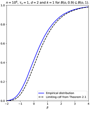
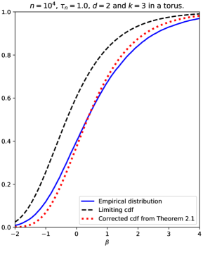
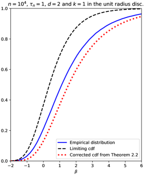
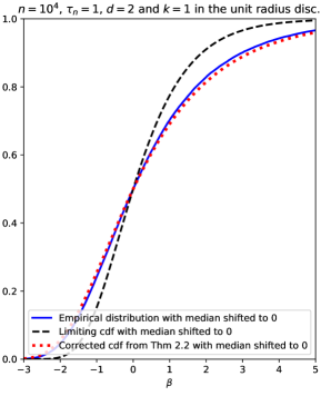
Figure 2: The empirical distributions of $n\theta_{d}f_{0}R_{n,m(n),k}^{d}-c_{1}\log n-c_{2}\log\log n$ obtained from computer simulations in the settings of Theorems 2.1, 2.2 and 2.3, plotted on the same axes as the limiting distributions. See Section 6 for discussion of the simulation results.

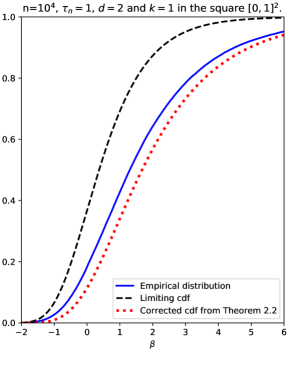
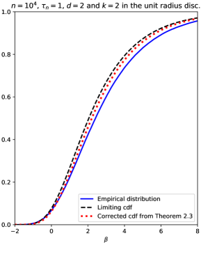
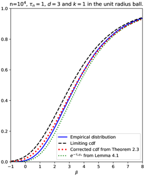
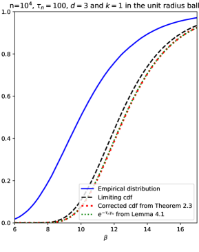
Figure 3: The continuation of Figure 2, with results from simulations in several more settings.

We were able to write computer simulations which sample from the distribution of $R_{n,m(n),k}$ using a very simple algorithm: sample $n+m(n)$ independent points $X_{1},\dots,X_{n},Y_{1},\dots,Y_{m(n)}$. For each $j\in\{1,\dots,m(n)\}$ let $d_{j}^{(k)}$ be the Euclidean distance between $Y_{j}$ and its $k$th-nearest point in $\mathcal{X}_{n}=\{X_{1},\cdots,X_{n}\}$. Then $R_{n,m(n),k}=\max_{j\leq m(n)}d_{j}^{(k)}$.

In Figures 2 and 3, we present the results from simulations of many of the settings for which we have proved limit theorems. In each of the eight plots, the blue curve is an estimate of the cumulative distribution function of the quantity of the form $n\theta_{d}f_{0}R_{n,m(n),k}^{d}-c_{1}\log n-c_{2}\log\log n$ for which we have obtained weak laws. These distributions were estimated by sampling several tens of thousands of times from the distribution of $R_{n,m(n),k}$ and plotting the resulting empirical distribution. The black dashed curves are the corresponding limiting distributions as $n\to\infty$, from Theorems 2.1, 2.2 and 2.3. The red dotted curves are the corresponding “corrected” distributions, i.e. the explicit distributions which occur on the right-hand side of the expressions in our limit theorems, neglecting only the errors of order $(\log n)^{-1}$.

The top row in Figure 2 shows two cases covered by Theorem 2.1. The top-left diagram is for $B=B(o,0.9)$, $A=B(o,1)$, which meets condition A3. We have $d=2$ and $k=1$, so there is no “correction” to the limiting distribution. This is the only diagram in which we have taken $n$ larger than $10^{4}$. When plotted for $n=10^{4}$ (not pictured), the distance between the empirical distribution and the limiting distribution appears to be smaller than for $n=10^{6}$, but the shapes of the curves are very different, indicating that there is still a boundary effect influencing the distribution of the two-sample coverage threshold.

The top-right diagram is for our results when points are placed on the 2-dimensional unit torus. As a remark following Theorem 2.1 states, the proof of that theorem would generalise to this setting, giving exactly the same result. We have simulated $R_{n,m(n),k}$ for $k=3$, which is a case covered by our Theorem 2.1 but not included in the results of [3].

Both diagrams on the bottom row of Figure 2 are representations of the same simulation, with points placed inside the two-dimensional unit disc, which certainly has a smooth boundary. The inclusion of the explicit term of order $(\log n)^{-1/2}$ improves the accuracy of the estimated distribution considerably, as can be seen from the fact that the red dotted curve in the left diagram is much closer to the empirical distribution than the black dashed curve. In this $d=2$, $k=1$ setting the correction is of a larger order than the $O(\frac{\log\log n}{\log n})$ terms in all of the other settings.

We remarked after stating Theorem 2.2 that $n\pi f_{0}R_{n,m(n)}^{2}-\mu(n\pi f_{0}R_{n,m(n)}^{2})\stackrel{{\scriptstyle{\cal D}}}{{\longrightarrow}}{\mathsf{Gu}}_{\log\log 2,1}$, where $\mu(\cdot)$ is the median and ${\mathsf{Gu}}_{\log\log 2,1}$ is a Gumbel distribution with scale parameter 1 and median 0. To illustrate this, in the second diagram on the second row of Figure 2 we have translated all of the curves from the first diagram so that they pass through $(0,1/2)$, i.e. so that they are the distributions of random variables with median $0$. We can see that the corrected distribution is very close to the empirical distribution from the simulation, indicating that the shape of the corrected limiting distribution closely matches the actual distribution of $n\pi f_{0}R_{n,m(n)}^{2}$ for finite $n$, but with an offset corresponding to the difference between $\log n$ and the median of $n\pi f_{0}R_{n,m(n)}^{2}$.

In the setting of Theorem 2.2, the presence of a boundary has an effect on the distribution of $n\pi f_{0}R_{n,m(n)}^{2}$ which disappears as $n\to\infty$, so is not reflected in the limit. Broadly speaking, the terms involving $e^{-\beta}$ come from the interior, and terms involving $e^{-\beta/2}$ come from the boundary. Our correction term corrects the shape of the distribution to account for these boundary effects.

The blue curve in the left-hand diagram was translated by the sample median in order to pass through $(0,1/2)$ in the right-hand diagram. However, for applications of these limit theorems to real data, it is unlikely that tens of thousands of independent samples of $R_{n,m}$ will be available to estimate the median of the distribution.

Theorem 2.2 covers two cases for $d=2$, $k=1$: when $A$ has a smooth boundary, and when $A$ is a polygon. The first diagram in Figure 3 is in this latter case, with $A=[0,1]^{2}$. If we compare this diagram with the bottom-left diagram of Figure 2, which is also for $d=2$, $k=1$ but with $A=B(o,1)$, all of the same qualitative features can be observed: a fairly large gap between the empirical distribution and the limit, a large improvement due to the correction, and an “overshoot” so the corrected distribution approximates the empirical distribution from the right-hand side while the limiting distribution is to the left.

This indicates that the behaviour of the two-sample coverage threshold (at least in two dimensions) is not strongly affected by the presence of “corners” on the boundary of $A$. It is likely that in higher dimensions, the limiting behaviour of $R_{n,m(n)}$ when $A$ is a polytope would be different from the behaviour when $A$ has a smooth boundary, as was observed for the coverage threshold in [8].

The top-right diagram in Figure 3 is for $d=2$, $k=2$ with points inside the unit disc, which is the setting of the first limit result in Theorem 2.3. The $d=2$, $k=2$ case is unique in that the limiting distribution has two terms, corresponding to the boundary and interior. In the other settings the limiting distribution for the position of the point in $\mathcal{Y}_{j}$ which is last to be $k$-covered as the discs expand is either distributed according to Lebesgue measure on $A$, or according to a distribution supported on $\partial A$. However, the existence of both terms in the limit in (2.7) indicates that for $d=k=2$, the “hardest point to $k$-cover” has a mixed distribution: the sum of a measure supported on the interior of $A$ with a measure supported on $\partial A$.

The bottom row of Figure 3 contains the distributions from two simulations with $d=3$ and $k=1$ inside the unit ball. In the left diagram we have taken $\tau=1$, and the corrected limit approximates the empirical distribution well. In the right diagram we have taken $\tau=100$. The empirical distribution is extremely far from the limiting distribution, and the correction term has the wrong sign, so the corrected limit is an even worse approximation to the empirical distribution than the uncorrected limit is.

The fact that the empirical distribution is far to the left of the limit (i.e. that $R_{n,m(n),k}^{d}$ is generally smaller than the limit would predict) when $\tau$ is large is rather surprising. If we consider $\tau_{n}\uparrow\infty$ sufficiently fast as $n\to\infty$, then $R_{n,m(n),k}$ should approximate the coverage threshold considered in [8]. As we remarked after the statement of Theorem 2.3, the coverage threshold is generally much larger than our $R_{n,m(n),k}$. In the case $d=3$, $k=1$, the coefficient of $\log\log n$ in the weak law for the coverage threshold corresponding to Theorem 2.3 is larger, and so we might expect that if $\tau$ is large than the empirical distribution for $n\theta_{d}f_{0}R_{n,m(n),k}^{d}-(2-2/d)\log n-(2k-4+2/d)\log\log n$ in Figure 3 would be far to the right of the limiting distribution.

To explain the surprising fact that it is instead far to the left of the limit, we should examine Lemma 4.1. In the “Poissonised” setting of that Lemma, given the configuration of “transmitters” $\mathcal{X}_{t}$, the conditional probability ${\mathbb{P}}[R_{t,\tau t,k}^{\prime}\leq r_{t}|\mathcal{X}_{t}]$ is the probability that no point from $\mathcal{Y}_{\tau t}$ lies in the vacant region $V_{t,\tau t,k}$. The lemma shows that when we replace the marginal probability ${\mathbb{P}}[R_{t,\tau t,k}^{\prime}\leq r_{t}]$ with the probability that no point from $\mathcal{Y}_{\tau t}$ lies in a region of Lebesgue measure $\mathbb{E}\,V_{t,\tau t,k}$, the error induced is $O((\log t)^{1-d})$. However, this is for fixed $\tau$. It can be seen from the proof that the error is proportional to $\tau^{2}(\log t)^{1-d}$, which is not negligible unless $t$ is very large compared to $\tau$.

To see why the corrected limiting cdf is below the empirical cdf, let $f(x):=e^{-\tau x}$. In Lemma 4.1, if $\Gamma_{t}:=(t/|B|)|V_{t,r_{t},k}\cap B|$, then ${\mathbb{P}}[R_{t,\tau t,k}^{\prime}(B)\leq r_{t}]=\mathbb{E}\,[f(\Gamma)]$, while $e^{-\tau\gamma_{t}(B)}=f(\mathbb{E}\,[\Gamma])$. Hence by Jensen’s inequality, $e^{-\tau\gamma_{t}}$ can only ever be an underestimate for ${\mathbb{P}}[R_{t,\tau t,k}^{\prime}(B)\leq r_{t}]$, with an error proportional to $\tau^{2}$. All of our corrected expressions in Theorem 2.3 are approximations of $e^{-\tau\gamma_{t}}$.

If we think of $\mathcal{X}_{n}$ as a set of transmitters and $\mathcal{Y}_{m(n)}$ as a set of receivers, then for most applications we would expect $\tau_{n}$ to be large. It should be possible to improve the estimate in this case by computing the leading-order error terms in Lemma 4.1, using moments of $t|V_{t,\tau t,k}|$ or otherwise.

Acknowledgements. We thank Keith Briggs for suggesting this problem, and for some useful discussions regarding simulations.

Availability of Data and Materials declaration. The code for the simulations discussed in Section 6 is available at https://github.com/frankiehiggs/CovXY and the samples generated by that code are available at https://researchdata.bath.ac.uk/id/eprint/1359.

References

- [1] García Trillos, N., Slepčev, D. (2016). Continuum limit of total variation on point clouds. Arch. Ration. Mech. Anal. 220, 193–241.
- [2] Hall, P. (1985). Distribution of size, structure and number of vacant regions in a high-intensity mosaic. Z. Wahrsch. Verw. Gebiete 70, 237–261.
- [3] Iyer, S. and Yogeshwaran, D. (2012) Percolation and connectivity in AB random geometric graphs. Adv. Appl. Prob. 44, 21–41.
- [4] Janson, S. (1986). Random coverings in several dimensions. Acta Math. 156, 83–118.
- [5] Last, G. and Penrose, M. (2018). Lectures on the Poisson Process. Cambridge University Press, Cambridge.
- [6] Leighton, T. and Shor, P. (1989). Tight bounds for minimax grid matching with applications to the average case analysis of algorithms. Combinatorica 9, 161–187.
- [7] Penrose, M. D. (2014) Continuum AB percolation and AB random geometric graphs. J. Appl. Prob. 51A, 333–344.
- [8] Penrose, M. D. (2023) Random Euclidean coverage from within. Probab. Theory Related Fields 185, 747–814.
- [9] Penrose, M. (2003). Random Geometric Graphs. Oxford University Press.
- [10] Rossi, F., Fiorentino, M. and Versace, P. (1984) Two-component extreme value distribution for flood frequency analysis. Water Resources Research 20, 847–856.
- [11] Shor, P. W. and Yukich, J. E. (1991). Minimax grid matching and empirical measures. Ann. Probab. 19, 1338–1348.