Sub-Rayleigh ghost imaging via structured illumination

Abstract

The structured illumination adopted widely in super-resolution microscopy imaging works for the ghost imaging scheme also. Here, we studied the ghost imaging scheme with sinusoidal-structured speckle illumination, whose spatial resolution can surpass the Rayleigh resolution limit by a factor of 2. In addition, even if the bucket intensity signal originated from the diffraction of the object plane with a certain distance, the improvement of spatial resolution is still effective. Our research shows that the structural illumination method, an independent super-resolution technology, is expected to be grafted with a variety of super-resolution ghost imaging schemes to further improve the resolution of imaging systems, such as the pseudo-inverse ghost imaging.

I Introduction

Due to wave property and finite diffraction aperture, the incoherence imaging system is of limited imaging resolution, known as the Rayleigh-resolution limit [1] $\Delta x_{R}=0.61\lambda/\text{NA}$, where $\lambda$ is the wavelength of light and NA is the numerical aperture of imaging system  [2]. To break through the resolution limit, Heintzmann and Cremer have proposed a super-resolution imaging scheme in 1999 in which the object has been illuminated by a series of structured light-field created by grating diffraction with coherent light [3]. The detected spectrum by an imaging system will be shifted if the object has being illuminated by structured light, such as sinusoidal intensity pattern. Thus, the structured light illumination as a super-resolution technology is based on the perspective of the extended-spectrum domain [4, 5, 6]. Because of high photon efficiency and fast imaging speed, the structured illumination of super-resolution imaging technology has been applied to a wide variety of biological problems [7, 8], which gives birth to a hot topic the structured illumination microscopy (SIM). Moreover, due to simple experimental setup, SIM is compatible widely with other super-resolution imaging schemes [9, 10, 11] to create many hybrid super-resolution imaging technologies.

Similar to structured illumination imaging, the ghost imaging (GI) has also rely on light-field irradiating the imaging object. As a computational imaging technology, GI is originated from two-arms intensity correlation between a point-signal arm with a non-spatial resolution bucket (or single-pixel) detector which collects transmitted light from the imaging object, and a array-signal arm with a pixelated array of detector which never interacted with the object and only record the light-field distribution on the twin plane of the object’s plane. Actually, those twin planes, where light-field has exactly the same temporal and spatial distribution, can be create either quantum sources [12, 13, 14, 15] or classical sources with the help of a beam splitter (BS) [16, 17, 18, 19, 20, 21, 22, 23, 24, 25, 26, 27]. At first, people believed that only quantum sources can realize GI, but after a while the GI research with classical light became popular, such as artificial light sources [17, 20, 22], sun light [24, 25, 26], and even priori light sources [28, 27, 29, 30], etc. Remarkably, the GI scheme with a priori light source can be change into the one-arm computational ghost imaging (CGI) [31] because the array signal arm can be replaced by the artificial computational via the diffraction integral formula [2]. Interestingly, this simplified single-arm GI scheme [32, 31, 33, 34] has given birth to a novel research topic the single-pixel imaging (SPI) [35, 36, 37], which undoubtedly brings many advantages such as free of aberration caused by the multi-wavelength dispersion, wide spectral range detection, and higher detection signal noise ratio in weak light environment. As one of the key device, the spatial light modulator (SLM) can not only simplify the experimental device of GI to SPI [28, 27], but also be widely used in structured light imaging [38, 39, 40, 41, 42]. Consequently, a hybrid super-resolution imaging scheme between GI and structured illumination imaging is possible theoretically with the help of the SLM .

Similar to traditional incoherent imaging system, the spatial resolution of thermal GI also follows the Rayleigh-resolution limit [19, 23, 27]. For the far-field GI scheme, the numerical aperture $\text{NA}=\frac{\Delta L}{2z}$ is decided by the diameter $\Delta L$ of thermal source and the diffraction distance $z$ between the source and the imaging object. To improve the spatial resolution of GI system, some methods have been studied, such as compressed sensing [43, 44, 45], pseudo-inverse ghost imaging (PGI) [46, 47], non-Rayleigh speckle fields [48, 49], spatial filtering of the detected speckles [50, 51], optical fluctuation [36], and deep learning [52] etc. In this work, we reported a far-field sub-Rayleigh structured illumination ghost imaging (SGI) scheme with sinusoidal-structured speckle. Here, the sinusoidal-structured speckle can be obtained by holographic projection technology or the pseudo-modulation method. Comparing with the limited modulation frequency leading to a factor of 2 enhancement of the spatial resolution over the traditional ghost imaging by holographic projection, the pseudo-modulation method is unconstrained. In addition, the diffractive SGI scheme was also analyzed when the imaging object and the bucket detector are not close contact. Finally, a grafted super-resolution imaging scheme between SGI and PGI is discussed in detail.

II Theory

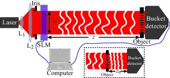
Figure 1: Schematic diagram of sub-Rayleigh single-pixel SGI. $\text{L}_{1}$, $\text{L}_{2}$: lenses; SLM: spatial light modulator. The inset at the right-bottom corner shows the diffractive SGI scheme with distance $z_{0}$ between the object plane and the bucket detector.

The experimental setup of SGI, depicted in Fig. 1, is identical with the CGI setup [31]. A computer-controlled phase-only SLM is used to modulate the wavefront of a laser beam to create the soure field $E(r_{\text{s}},t)=e^{i\theta(r_{\text{s}},t)}$, whose phasor $\theta(r_{\text{s}},t)$ is dynamic prepared in advance. Here, the effective aperture of $E(r_{\text{s}},t)$ is controlled by an iris with a diameter $\Delta L$. The source field $E(r_{\text{s}},t)$ undergos quasi monochromatic paraxial diffraction along the optical axe, over an $z$ free-space path, yielding the structured field $E(r_{\text{o}},t)$ on the object’s plane. In order to create far-field GI scheme, a lens phase factor $e^{-ikr_{s}^{2}/\left(2z\right)}$ is superposed on the phasor $\theta(r_{\text{s}},t)$ of source, where $k=2\pi/\lambda$ is the wave number. An amplitude transmission object $O(r_{\text{o}})$, located immediately in front of a single-pixel bucket photodetector, are illuminaged by the structured field $E(r_{\text{o}},t)$. Here, the traditional CGI is given by [19, 28, 53, 27]

$$\begin{split}GI{(r_{o})}=\frac{{\text{1}}}{{{N}}}\sum\limits_{i=1}^{N}{\left({I_{i}}{(r_{o})}-\left\langle{I{(r_{o})}}\right\rangle\right){BI_{i}}}\,,\end{split}$$ (1)

where $N$ is the number of total frames, ${I_{i}}{(r_{o})}=\left|E(r_{\text{o}},t)\right|^{2}$ is the $i$th frame array-signal namely the instantaneous intensity distribution on the object plane at $t$ time and $\left\langle{I{(r_{o})}}\right\rangle=\frac{1}{N}{\textstyle\sum_{i=1}^{N}}I_{i}\left(r_{o}\right)$ is the ensemble average of all instantaneous intensity, $BI_{i}=\int{I_{i}}{(r_{o})}O(r_{\text{o}})dr_{\text{o}}$ is the bucket signal which is the total light intensity passing through the object. Here, the $i$th frame phase $\theta_{i}(r_{\text{s}},t)$ prepared in advance will be loaded experimentally at time sequence $t$. Therefore, for a priori source field $E(r_{\text{s}},t)$, only a single-pixel bucket detector is essential to collect the transmission coefficient $BI_{i}$ to reconstruct the spatial distribution of the object’s projected transmission $O(r_{\text{o}})$ [31].

The matrix operations offers a concise way to express the correlation algorithm of GI. Provided that the speckle ${I_{i}}{(r_{o})}$ is composed of $m\times n$ pixels so that the speckle sequence ${I_{i}}(r_{o})$ ($i=1,2,\cdots,N$) creates the $N\times K$ ($K=m\times n)$ measurement matrix $\Phi_{(N\times K)}$, namely

$$\Phi=\left[\begin{array}[]{l}{I_{1}}\left({1,1}\right),{\kern 1.0pt}{I_{1}}\left({1,2}\right),{\kern 1.0pt}\cdots,{\kern 1.0pt}{I_{1}}\left({m,n}\right)\\ {I_{2}}\left({1,1}\right),{\kern 1.0pt}{I_{2}}\left({1,2}\right),{\kern 1.0pt}\cdots,{\kern 1.0pt}{I_{2}}\left({m,n}\right)\\ \quad\vdots\quad\quad\quad\ddots\\ {I_{N}}\left({1,1}\right),{\kern 1.0pt}{I_{N}}\left({1,2}\right),{\kern 1.0pt}\cdots,{\kern 1.0pt}{I_{N}}\left({m,n}\right)\end{array}\right].$$ (2)

Further, a matrix $\Psi_{(N\times K)}=\Phi_{(N\times K)}-{\text{E}_{(N\times 1)}}\left\langle\Phi\right\rangle_{(1\times K)}$ are defined, where ${\text{E}}_{(N\times 1)}$ is a $N\times 1$ row vector with all elements one and $\left\langle\Phi\right\rangle_{(1\times K)}{\rm{=}}\frac{1}{N}{\textstyle\sum_{i=1}^{N}}{\Phi_{i{(1\times K)}}}$ is the average of the measurement matrix in row direction. Here, ${\Phi_{i{(1\times K)}}}$ denotes the $i$th row vector of the matrix $\Phi_{(N\times K)}$. Therefore, the matrix format of Eq. (1) can be simply expressed [53, 47]:

$$GI=\frac{1}{N}{\Psi^{\text{T}}}\Phi O,$$ (3)

where $\Psi^{\text{T}}$ denotes the transposition of the matrix $\Psi$ and $O={\left[{o\left({1,1}\right),{\kern 1.0pt}o\left({1,2}\right),{\kern 1.0pt}\cdots,{\kern 1.0pt}o\left({m,n}\right)}\right]^{\rm{T}}}$ is the $K\times 1$ column vector which originates from the object $O(r_{\text{o}})$.

To realize SGI, the speckle are modulated by a series of sinusoidal intensity patterns

$$s\left({\vec{r}}_{o},\alpha,\beta,p\right)=1-m\cos\left(2\pi\overrightarrow{p_{\alpha}}\cdot\overrightarrow{r_{o}}+\beta\right),$$ (4)

where $\alpha\in A=\left[0,\pi/3,2\pi/3\right]$ indicates the orientation of sinusoidal illumination pattern, $\beta\in B=\left[0,2\pi/3,4\pi/3\right]$ is phase of illumination pattern, $m$ is the modulation factor, $\overrightarrow{p_{\alpha}}=(p\cos\alpha{\vec{i}},p\sin\alpha{\vec{j}})$ is sinusoidal illumination frequency vector in reciprocal space, and ${{\vec{r}}_{o}}=({{x_{o}}\vec{i},{y_{o}}\vec{j}})$ is the coordinates of object plane, respectively. Generally speaking, the maximum of the amplitude of sinusoidal frequency vector $p$ is $\frac{1}{\Delta x_{R}}$. Moreover, $s\left({\vec{r}}_{o},\alpha,\beta,p\right)$ can also act as an $m\times n$ matrix which can create a $K\times K$ diagonal matrix vector

$$S\left(\alpha,\beta,p\right)=\left[\begin{array}[]{l}{s\left(1,1,\alpha,\beta,p\right)},0,\cdots,{\kern 1.0pt}0\\ 0\,,{s\left(1,2,\alpha,\beta,p\right)},\cdots,0\\ \;\vdots\quad\;\;\;\;\;\ddots\;\;\quad\;\;\;{\kern 1.0pt}\;\quad\quad\vdots\\ 0,0,\cdots,{s\left(m,n,\alpha,\beta,p\right)}\end{array}\right].$$ (5)

Therefore, the matrix operations of SGI when the speckle modulated by the sinusoidal intensity patterns $s\left({\vec{r}}_{o},\alpha,\beta,p\right)$ can be expressed as

$$sgi\left(\alpha,\beta,p\right)=\frac{1}{N}{\Psi^{\text{T}}}M\left(\alpha,\beta,p\right)O,$$ (6)

where $M\left(\alpha,\beta,p\right)=\Phi S\left(\alpha,\beta,p\right)$ is the matrix of the speckle modulated by the sinusoidal patterns. Comparing with the matrix operations of traditional GI shown by the Eq. (3), it can be seen that the only difference of the SGI is the sinusoidal structured speckle illumination replaces the original speckle field only in the bucket detector signal arm. This sinusoidal structured speckle can be created by the free diffraction of the computer-generated holography (CGH) which created by the Gale-Shapley (GS) algorithm in advance. In fact, if a charge coupled device (CCD) acts as the bucket detector in the SGI scheme [27], this sinusoidal intensity modulated speckle field can be achieve by a subsequent data processing. Accroding to the structured illumination image reconstruction algorithm [54], the SGI with illumination frequency vector $p$ can be create by

$$SGI(p)=\mathop{\Upsilon}\limits_{\left({\alpha,\beta}\right)\in\Omega}\{{sgi\left({\alpha,\beta,p}\right)}\},$$ (7)

where the operator $\Upsilon$ means the spectrum connectton by those sub-images $sgi\left(\alpha,\beta,p\right)$, and the modulation set $\Omega$ originates from the Cartesian product $A\times B=\left\{(\alpha,\beta)|\alpha\in A,\beta\in B\right\}$. In the Sec. III and Sec. IV, we averaged those spectrum, calculated from those sub-images, at overlapping regions to build the SGI, which is the meaning of the operator $\Upsilon$.

In some ghost imaging schemes, there is a distance between the object and the bucket detector as shown by the inset in Fig. 1. At this moment, the bucket detector just collects the diffraction signal of the transmitted speckle from the imaging object. Therefore, the matrix format of the diffraction GI can be expressed:

$$GI_{D}=\frac{1}{N}{\Psi^{\text{T}}}\bigtriangleup\{\Phi O\},$$ (8)

where the operator $\bigtriangleup$ means the free diffraction and $\bigtriangleup\{\Phi O\}$ is the bucket signal originated from the free diffraction of $\Phi O$. Similarly, the diffraction SGI can be acquired by

$$SGI_{D}(p)=\mathop{\Upsilon}\limits_{\left({\alpha,\beta}\right)\in\Omega}\{{sgi_{D}\left({\alpha,\beta,p}\right)}\},$$ (9)

where

$$sgi_{D}\left(\alpha,\beta,p\right)=\frac{1}{N}{\Psi^{\text{T}}}\bigtriangleup\{M\left(\alpha,\beta,p\right)O\}.$$ (10)

In the following sections, we will verify the high spatial resolution ability of those SGI schemes.

III Numerical Experiment

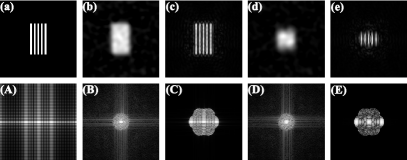
Figure 2: (a) Test object. (b) Non-diffractive GI. (c) Non-diffractive SGI. (d) Diffractive GI. (e) Diffractive SGI. (A,B,…,E) Logarithmic transformation of Fourier domain of images in (a,b,…,e), respectively.

Figure 1 depicts the experimental setup to demonstrate the high-resolution ability of SGI. A continuous-wave $\lambda$ = 532 nm single-mode laser beam was expanded and collimated by two lenses $L_{1}$ and $L_{2}$, and then passed through an iris and a phase-only SLM (an element pixel size of 20 × 20 $\mu\text{m}^{2}$ and a total pixels 512 $\times$ 512). The iris was placed as close as possible to the SLM, and its diameter $\Delta L$ was set to be 1.2 mm. For simplicity, only one-dimensional case is considered, and extension to the two-dimensional case is straight forward. To generate the dynamic speckle illumination, the phase structure $e^{i\theta(r_{\text{s}},t)-ikr_{s}^{2}/(2z)}$ were loaded on the SLM, where the phasor $\theta(r_{\text{s}},t)$ is completely random in the time and spatial distribution, $z$ = 0.8 m is the distance between the object plane and the SLM, respectively. Therefore, the Rayleigh-resolution limit $\Delta x_{R}$ of non-diffractive GI scheme, the bucket detector was placed as close as possible to the object, is 433 $\mu\text{m}$. Here, the size of the bucket detector is larger than the object. For the diffractive GI scheme as shown by the inset in the Fig. 1, the diffractive distance $z_{0}$ is 0.5 m between the bucket detector and the object. Here, the size of the bucket detector is 0.6 mm.

To test the high-resolution ability of SGI, we perform the follow-up numerical experiments with Matlab to compare the non-diffractive/diffractive SGI with the corresponding GI as shown in Fig. 2. Here the number of total frames $N$ is 10000 for GI scheme and SGI scheme. We choose a 0-1 resolution test object with 256×256 pixels, which consists alternative opaque and clear stripes of equal width as shown in Fig. 2(a). As expected, stripes of the text object are indistinguishable in the non-diffractive GI scheme as shown by the Fig. 2(b), due to the spatial resolution of non-diffractive GI scheme much larger than the spacing 250 $\mu\text{m}$ of adjacent fringe in the text object. On the other hand, all stripes in the object are distinguishable in the SGI scheme as shown by the Fig. 2(c). In theory, the spatial resolution of SGI scheme is $\Delta x_{R}/2=216.5$ $\mu\text{m}$. In addition, compared with the diffractive GI as shown by the Fig. 2(d), the diffractive SGI scheme also improves the imaging quality as shown by the Fig. 2(e). To illustrat the extended-spectrum by SGI scheme, figures 2 (A,B,…,E) present the logarithmic transformation $\text{log}\left(1+\left|\mathscr{F}\left(\text{image}\right)\right|\right)$ of Fourier domain of images in figures 2 (a,b,…,e), respectively. It can be seen that the effective spectrum of SGI scheme is larger than the corresponding GI schemes.

The fidelity of imaging can also be estimated by calculating the peak signal-to-noise ratio (PSNR):

$$\begin{split}PSNR=10\log_{10}{\left[{{({2^{\text{B}}-1})}^{2}}/MSE\right]},\end{split}$$ (11)

where $\text{B}=8$ is the bit depth of images and $MSE$ is the mean-square error of the result with respect to the test object, which is defined as:

$$\begin{split}MSE=\frac{1}{N^{2}}\sum\limits_{i=1}^{\tau}\sum\limits_{j=1}^{\tau}{\left[GI(i,j)-O(i,j)\right]^{2}},\end{split}$$ (12)

where the result of ghost imaging $GI(i,j)$ and the test object $O(i,j)$ are digitized to $0\sim 2^{\text{B}}-1$, $i,j$ are the index of the pixel and $\tau=256$ is the total number of pixels in single dimension, respectively. It can be seen that the higher the quality of the result, the greater the PSNR. According to the experimental results, the PSNRs of Fig. 2(b-e) are 5.9 dB, 12.5 dB, 6.6 dB and 7.0 dB, respectively. It can be seen that the quality of ghost image results has been optimized through structured illumination method.

IV Discussion

IV.1 the structured ghost imaging with the pseudo-modulation

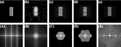
Figure 3: (a) Test object. (b) GI. (c) SGI. (d) Pseudo-modulation SGI. (e) PGI. (A,B,…,E) Logarithmic transformation of Fourier domain of images in (a,b,…,e), respectively.

Actually, in addition to authentic speckle modulation by CGH, a pseudo-modulation of speckle structured illumination with frequency vector $p^{\prime}$ is effective for non-diffractive SGI, which can be available by

$$S_{pse}GI(p^{\prime})=\mathop{\Upsilon}\limits_{\left({\alpha,\beta}\right)\in\Omega^{\prime}}\{{s_{pse}gi\left({\alpha,\beta,p^{\prime}}\right)}\},$$ (13)

where

$$s_{pse}gi\left(\alpha,\beta,p^{\prime}\right)=\frac{1}{N}{\Psi^{\text{T}}}M\left(\alpha,\beta\right){\Phi^{-1}}\Phi O.$$ (14)

Here, $\Phi^{-1}$ is the Moore–Penrose pseudo-inverse of the measurement matrix $\Phi$. It can be seen that, as long as the transmission coefficient array $\Phi O$ is available by the bucket detector, arbitrary modulation frequency $p^{\prime}$ and arbitrary modulation orientation $\left(\alpha,\beta\right)$ of structural illumination can be achieved in the pseudo-modulation SGI scheme, which can break the upper limit of modulation frequency in traditional structured illumination optical system. For the pseudo-modulation SGI, we connectton the spectrum of three sets of structural illumination $\left({{\rm{A^{\prime}}}\times{\rm{B}},2p/\sqrt{3}}\right)$, $\left({{\rm{A}}\times{\rm{B}},2p}\right)$, and $\left({{\rm{A^{\prime}}}\times{\rm{B}},4p/\sqrt{3}}\right)$, respectively. Here, a new orientation of sinusoidal illumination pattern ${{\rm{A^{\prime}}}}$ is $\left[\pi/6,3\pi/6,5\pi/6\right]$. Therefore, the spatial resolution of pseudo-modulation SGI scheme will be better than the SGI scheme in theory.

Actually, the pseudo-modulation SGI scheme has some similarities with the pseudo-inverse ghost imaging (PGI) [47]. According to the imaging algorithm of PGI scheme ($PGI=\frac{1}{N}\Psi^{\text{-1}}\Psi O$), the spectrum of pseudo-modulation SGI is only a subset of PGI’s so that the pseudo-modulation SGI has a poorer spatial resolution than PGI scheme. Nevertheless, the pseudo-modulation SGI demonstrates indirectly the sub-Rayleigh spatial resolution of PGI scheme.

Figure 3 shows the numerical simulation demonstration of spatial resolution superiority of the pseudo-modulation SGI than the SGI. Here the number of total frames $N$ is 2000 for those non-diffractive GI variant scheme. Figure 3 (a) show the test object with the spacing 167 $\mu\text{m}$ of adjacent fringe. Using the same imaging methods as in Fig. 2 (b) and Fig. 2 (c), the imaging results of GI and SGI are shown in the Fig. 3 (b) and Fig. 3 (c), respectively. Figure 3 (d) show the pseudo-modulation SGI, whose maximum frequency limit of imaging scheme is $3p$. What’ more, figure 3 (e) shows the PGI. Figures 3 (A,B,…,E) present the logarithmic transformation $\text{log}\left(1+\left|\mathscr{F}\left(\text{image}\right)\right|\right)$ of Fourier domain of images in figures 3 (a,b,…,e), respectively. Compared to SGI scheme, the pseudo-modulation SGI scheme has significantly better spatial resolution. Although the imaging quality of PGI scheme is better than other schemes, there is inevitable white noise except the low-frequency region. Therefore, the extended spectrum of low-frequency region of structured illumination PGI will be beneficial for the ghost imaging quality. This will be discussed in the following section.

IV.2 the structured ghost imaging combined with the PGI scheme

To further optimize the imaging quality, two types of sub-Rayleigh imaging schemes the SGI and the PGI can be combined to create the structured illumination pseudo-inverse ghost imaging (SPGI), which can be available by

$$SPGI(p)=\mathop{\Upsilon}\limits_{\left({\alpha,\beta}\right)\in\Omega}\{spgi\left({\alpha,\beta,p}\right)\},$$ (15)

where

$$spgi\left(\alpha,\beta,p\right)=\frac{1}{N}{\Psi^{\text{-1}}}M\left(\alpha,\beta,p\right)O.$$ (16)

What’s more, a pseudo-modulation SPGI scheme with three sets of structural illumination $\left({{\rm{A^{\prime}}}\times{\rm{B}},2p/\sqrt{3}}\right)$, $\left({{\rm{A}}\times{\rm{B}},2p}\right)$, and $\left({{\rm{A^{\prime}}}\times{\rm{B}},4p/\sqrt{3}}\right)$ can be available by

$$S_{pse}PGI(p^{\prime})=\mathop{\Upsilon}\limits_{\left({\alpha,\beta}\right)\in\Omega^{\prime}}\{s_{pse}pgi\left({\alpha,\beta,p^{\prime}}\right)\},$$ (17)

where

$$s_{pse}pgi\left(\alpha,\beta,p^{\prime}\right)=\frac{1}{N}{\Psi^{\text{-1}}}M\left(\alpha,\beta,p^{\prime}\right){\Phi^{-1}}\Phi O.$$ (18)

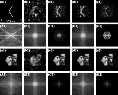
Figure 4: (a1)-(a2): Test object. (b1)-(b2): GI. (c1)-(c2): Pseudo-modulation SPGI. (d1)-(d2): PGI. (e1)-(e2): SPGI. (A1, A2, B1, B2,…, E1, E2) Logarithmic transformation of Fourier domain of images in (a1, a2, b1, b2,…, e1, e2), respectivley.

To demonstrate the super-resolution capability of the SPGI and the pseudo-modulation SPGI methods, figure 4 gives the numerical experiment with a 0-1 binary object ’K’ and a natural grayscale object Cameraman. For the imaging with the binary object, the number of total frames $N$ is 100, but $N$ is 500 for the grayscale object. Figures 4 (a1-a2) show those test objects. Using the same imaging methods as in Fig. 3 (b) and Fig. 3 (e), the imaging results of GI and PGI are shown in the Figs. 4 (b1-b2) and Figs. 4 (d1-d2), respectively. Compared with the GI, the PGI produces an better imaging quality. What’s more, the imaging results of the pseudo-modulation SPGI and the (authentic-modulation) SPGI are shown in the Figs. 4 (c1-c2) and Figs. 4 (e1-e2), respectively. Compared with the PGI, the pseudo-modulation SPGI does not achieves the optimization of ghost image quality but the (authentic-modulation) SPGI scheme achieves the goal. In fact, these results can been demonstrated in the spectrum domain. Figures 4 (A1, A2, B1, B2,…, E1, E2) present the logarithmic transformation $\text{log}\left(1+\left|\mathscr{F}\left(\text{image}\right)\right|\right)$ of Fourier domain of images in figures 4 (a1, a2, b1, b2,…, e1, e2), respectivley. For the pseudo modulation PGI, the detected spectrum as shown by the Figs. 4 (C1-C2) can not be shifted with pseudo modulation speckle illumination. However, the detected spectrum as shown by the Figs. 4 (E1-E2) can be shifted in the authentic-modulation SPGI scheme and leads to an better image quality than the PGI scheme.

V Conclusion

In conclusion, we proposed theoretically and demonstrated numerical experimentally the sub-Rayleigh SGI scheme. What’s more, a pseudo-modulation SGI scheme, whose modulation frequency breaks the upper limit of imaging system, can achieve a better imaging quality. Finally, we combined the SGI scheme and the PGI scheme and propose the SPGI scheme which can greatly enhance the ghost imaging quality whether the 0-1 binary object or a natural grayscale object.

References

- [1] J. W. Strutt, Philos. Mag. Series 5 8, 261 (1879).
- [2] J. Goodman, Introduction to Fourier Optics (McGraw-Hill, New York, 1995).
- [3] R. Heintzmann and C. G. Cremer, Proc. SPIE 3568, 185 (1999).
- [4] M. G. L. Gustafsson, J. Microsc. 198, 82 (2000).
- [5] M. G. L. Gustafsson, D. A. Agard, and J. W. Sedat, Proc. SPIE 3919, 141 (2000).
- [6] J. T. Frohn, H. F. Knapp, and A. Stemmer, Proc. Natl. Acad. Sci. USA 97, 7232 (2000).
- [7] R. Heintzmann, and T. Huser, Chem. Rev. 117, 13890 (2017).
- [8] F. Ströhl and C. F. Kaminski, Optica 3, 667 (2016).
- [9] H. Zhang, M. Zhao, and L. Peng, Opt. Express 19, 24783 (2011).
- [10] Y. Xue and Peter T. C. So, Opt. Express 26, 20920 (2018).
- [11] A. Bezryadina, J. Zhao, and Z. Liu, Conference on Lasers and Electro-Optics (CLEO) (2018).
- [12] D. N. Klyshko, Phys. Lett. A 128, 133 (1988).
- [13] T. B. Pittman, Y. H. Shih, D. V. Strekalov, and A. V. Sergienko, Phys. Rev. A 52, R3429 (1995).
- [14] A. F. Abouraddy, P. R. Stone, A. V. Sergienko, B. E. A. Saleh, and M. C. Teich, Phys. Rev. Lett. 93, 213903 (2004).
- [15] R. S. Aspden, N. R. Gemmell, P. A. Morris, D. S. Tasca, L. Mertens, M. G. Tanner, R. A. Kirkwood, A. Ruggeri, A. Tosi, R. W. Boyd, G. S. Buller, R. H. Hadfield, and M. J. Padgett, Optica 2, 1049 (2015).
- [16] R. S. Bennink, S. J. Bentley, and R. W. Boyd, Phys. Rev. Lett. 89, 113601 (2002).
- [17] A. Valencia, G. Scarcelli, M. D’Angelo, and Y. Shih, Phys. Rev. Lett. 94, 063601 (2005).
- [18] D.-Z. Cao, J. Xiong, and K. Wang, Phys. Rev. A 71, 013801 (2005).
- [19] F. Ferri, D. Magatti, A. Gatti, M. Bache, E. Brambilla, and L. A. Lugiato, Phys. Rev. Lett. 94, 183602 (2005).
- [20] D. Zhang, Y.-H. Zhai, L.-A. Wu, and X.-H. Chen, Opt. Lett. 30, 2354 (2005).
- [21] F. Ferri, D. Magatti, V. G. Sala, and A. Gatti, Appl. Phys. Lett. 92, 261109 (2008).
- [22] H. Liu, X. Shen, D.-M. Zhu, and S. Han, Phys. Rev. A 76, 053808 (2007).
- [23] X.-H. Chen, I. N. Agafonov, K.-H. Luo, Q. Liu, R. Xian, M. V. Chekhova, and L.-A. Wu, Opt. Lett. 35, 1166 (2010).
- [24] S. Karmakar, R. Meyers, and Y. Shih, in Quantum Communications and Quantum Imaging X, edited by R. E. Meyers, Y. Shih, and K. S. Deacon, SPIE Proc. Vol. 8518 (SPIE, Bellingham, 2012).
- [25] X.-F. Liu, X.-H. Chen, X.-R. Yao, W.-K. Yu, G.-J. Zhai, and L.-A. Wu, Opt. Lett. 39, 2314 (2014).
- [26] S. Karmakar, J. Opt. Technol, 87, 405 (2020).
- [27] L. Li, P. Hong, and G. Zhang, Phys. Rev. A 99, 023848 (2019).
- [28] Y. Bromberg, O. Katz, and Y. Silberberg, Phys. Rev. A 79, 053840 (2009).
- [29] Z.-H. Xu, W. Chen, J. Penuelas, M. Padgett, and M.-J. Sun, Opt. Express 26, 2427 (2018).
- [30] B. Sun, M. P. Edgar, R. Bowman, L. E. Vittert, S. Welsh, A. Bowman, and M. J. Padgett, Science 340, 844 (2013).
- [31] J. H. Shapiro, Phys. Rev. A 78, 061802 (2008).
- [32] L. Basano and P. Ottonello, Opt. Express 19, 12386 (2007).
- [33] A.-X. Zhang, Y.-H. He, L.-A. Wu, L.-M. Chen, and B.-B. Wang, Optica 5, 374 (2018).
- [34] T. Shimobaba, Y. Endo, T. Nishitsuji, T. Takahashi, Y. Nagahama, S. Hasegawa, M. Sano, R. Hirayama, T. Kakue, A. Shiraki, and T. Ito, Opt. Commun. 413, 147 (2018).
- [35] M. P. Edgar, G. M. Gibson, and M. J. Padgett, Nat. Photonics 13, 13 (2019).
- [36] P. Hong, Opt. Lett. 44, 1754 (2019).
- [37] M.-J. Sun and J.-M. Zhang, Sensors 19, 732 (2019).
- [38] P. Kner, B. B Chhun, E. R Griffis, L. Winoto, and M. L. G. Gustafsson, Nat. Methods 6, 339 (2009).
- [39] L. M. Hirvonen, K. Wicker, O. Mandula, and R. Heintzmann, Eur. Biophys. J. 38, 807 (2009).
- [40] B.-J. Chang, L.-J. Chou, Y.-C. Chang, and S.-Y. Chiang, Opt. Express 17, 14710 (2009).
- [41] K. Zhanghao, X. Chen, W. Liu, M. Li, Y. Liu, Y. Wang, S. Luo, X. Wang, C. Shan, H. Xie, J. Gao, X. Chen, D. Jin, X. Li, Y. Zhang, Q. Dai and P. Xi, Nat. Commun. 10, 4694 (2019).
- [42] Y. Guo, D. Li, S. Zhang, Y. Yang, J.-J. Liu, X. Wang, C. Liu, D. E. Milkie, R. P. Moore, U. S. Tulu, D. P. Kiehart, J. Hu, J. Lippincott-Schwartz, E. Betzig, and D. Li, Cell 175, 1430 (2018).
- [43] Y. Shechtman, S. Gazit, A. Szameit, Y. C. Eldar, and M. Segev, Opt. Lett. 35, 1148 (2010).
- [44] W. Gong, and S. Han, Sci. Reports, 5, 9280 (2015).
- [45] R. Zhu, G. Li, and Y. Guo, Int. J. Theor. Phys. 58, 1215 (2019).
- [46] C. Zhang, S. Guo, J. Cao, J. Guan, and F. Gao, Opt. Express 22, 30063 (2014).
- [47] W. Gong, Photon. Res. 3, 234 (2015).
- [48] S. Zhang, W. Wang, R. Yu, and X. Yang, Laser Phys. 26, 055007 (2016)
- [49] K. Kuplicki and K. W. C. Chan, Opt. Express 24, 26766 (2016).
- [50] J. Sprigg, T. Peng, and Y. Shih, Sci. Reports, 6, 38077 (2016).
- [51] S.-Y. Meng, Y.-H. Sha, Q. Fu, Q.-Q. Bao, W.-W. Shi, G.-D. Li, X.-H. Chen, and L.-A. Wu, Opt. Lett. 43, 4759 (2018)
- [52] F. Wang, C. Wang, M. Chen, W. Gong, Y. Zhang, S. Han, and G. Situ, Light Sci. Appl. 11, 1 (2022).
- [53] O. Katz, Y. Bromberg, and Y. Silberberg, Appl. Phys. Lett. 95, 131110 (2009).
- [54] A. Lal, C. Shan, and P. Xi, IEEE J. Sel. Top. Quantum Electron. 22, 50 (2016).