Optimal Differentially Private PCA and Estimation for Spiked Covariance Matrices

Abstract

Estimating a covariance matrix and its associated principal components is a fundamental problem in contemporary statistics. While optimal estimation procedures have been developed with well-understood properties, the increasing demand for privacy preservation introduces new complexities to this classical problem. In this paper, we study optimal differentially private Principal Component Analysis (PCA) and covariance estimation within the spiked covariance model.

We precisely characterize the sensitivity of eigenvalues and eigenvectors under this model and establish the minimax rates of convergence for estimating both the principal components and covariance matrix. These rates hold up to logarithmic factors and encompass general Schatten norms, including spectral norm, Frobenius norm, and nuclear norm as special cases.

We introduce computationally efficient differentially private estimators and prove their minimax optimality, up to logarithmic factors. Additionally, matching minimax lower bounds are established. Notably, in comparison with existing literature, our results accommodate a diverging rank, necessitate no eigengap condition between distinct principal components, and remain valid even if the sample size is much smaller than the dimension.

1 Introduction

The covariance structure plays a fundamental role in multivariate analysis, and Principal Component Analysis (PCA) is a widely recognized technique known for its efficacy in dimension reduction and feature extraction (Anderson, 2003). PCA is particularly adept in settings where the data is high-dimensional but the underlying signal displays a low-dimensional structure. The estimation of covariance matrices and principal components finds applications across a diverse spectrum, encompassing tasks such as image recognition, data compression, clustering, risk management, portfolio allocation, mean tests, independence tests, and correlation analysis. Methodologies and theoretical advancements, including minimax optimality, for covariance matrix estimation and PCA, have been well-established in both low-dimensional and high-dimensional settings. See, for example, Koltchinskii and Lounici (2017); Vershynin (2012); Srivastava and Vershynin (2013); Bickel and Levina (2008); Cai et al. (2010); Ravikumar et al. (2011); Johnstone (2001); Cai et al. (2013, 2015); Zhang et al. (2022). For a survey on optimal estimation of high-dimensional covariance structures, see Cai et al. (2016).

Amidst the increasing availability of large datasets containing sensitive personal information, privacy concerns in statistical data analysis have gained heightened prominence. The utilization of personal information in statistical analyses raises apprehensions about the potential compromise of individual privacy. Consequently, there is a growing emphasis on developing methodologies and techniques that offer robust privacy guarantees while still facilitating accurate statistical insights. This motivates a comprehensive exploration of the optimal tradeoff between privacy and accuracy in fundamental statistical problems, including PCA and covariance matrix estimation.

Differential privacy (DP), a concept introduced by Dwork et al. (2006), provides a framework for safeguarding individual privacy in statistical analysis. DP has become a commonly accepted standard in both industrial and governmental applications (Erlingsson et al., 2014; Ding et al., 2017; Apple Differential Privacy Team, 2017; Abowd, 2016; Abowd et al., 2020). The goal of the present paper is to develop methods and optimality results for PCA and covariance matrix estimation within the framework of the spiked covariance model under DP constraints.

1.1 Problem formulation

We begin by formally introducing the spiked covariance model and general formulation of the privacy constrained estimation problems.

The spiked covariance structure (Johnstone, 2001; Johnstone and Lu, 2009) naturally arises from factor models with homoscedastic noise and has found diverse applications in signal processing, chemometrics, econometrics, population genetics, and various other fields. See, for example, Fan et al. (2008); Kritchman and Nadler (2008); Onatski (2012); Patterson et al. (2006). The spiked covariance model assumes that the population covariance matrix can be decomposed as

$$\Sigma=U\Lambda U^{\top}+\sigma^{2}I_{p},$$ (1)

where $U\in\mathbb{O}_{p,r}$ and $\Lambda={\rm diag}(\lambda_{1},\cdots,\lambda_{r})$ represent the leading eigenvectors and eigenvalues (excluding $\sigma^{2}$), respectively. Here, $\mathbb{O}_{p,r}$ denotes the set of $p\times r$ matrices satisfying $U^{\top}U=I_{r}$. The spiked covariance model is convenient for studying the distribution of sample eigenvalues and eigenvectors, which play a critical role in the statistical inference of $\Sigma$ and its eigenvectors. For instance, Donoho et al. (2018) studied the optimal shrinkage of sample eigenvalues in the spiked covariance model. In particular, Cai et al. (2015) and Zhang et al. (2022) established the minimax optimal rates

$$\inf_{\widehat{U}}\sup_{\Sigma\in\Theta(\lambda,\sigma^{2})} \mathbb{E}\|\widehat{U}\widehat{U}^{\top}-UU^{\top}\|\asymp\bigg{(}\frac{\sigma^{2}}{\lambda}+\sqrt{\frac{\sigma^{2}}{\lambda}}\bigg{)}\sqrt{\frac{p}{n}};$$ (2)

$$\inf_{\widehat{\Sigma}}\sup_{\Sigma\in\Theta(\lambda,\sigma^{2})} \mathbb{E}\|\widehat{\Sigma}-\Sigma\|\asymp\lambda\sqrt{\frac{r}{n}}+\sqrt{\sigma^{2}(\lambda+\sigma^{2})}\sqrt{\frac{p}{n}},$$

where the infimum is taken over all possible estimators using the data set $X=(X_{1},\cdots,X_{n})$ consisting of $n$ observations sampled independently from the spiked covariance model (1) , the parameter set $\Theta(\lambda,\sigma^{2})$ is defined in (4) with $\lambda$ being the magnitudes of eigenvalues, and $\|\cdot\|$ denotes the matrix spectral norm.

The concept of differential privacy was first introduced in Dwork et al. (2006). For a given dataset $X$ and any $\varepsilon>0$ and $\delta\in[0,1)$, a randomized algorithm $A$ that maps $X$ into $\mathbb{R}^{d_{1}\times d_{2}}$ is called $(\varepsilon,\delta)$-differentially private ($(\varepsilon,\delta)$-DP) over the dataset $X$ if

$$\mathbb{P}\big{(}A(X)\in\mathcal{Q}\big{)}\leq e^{\varepsilon}\mathbb{P}\big{(}A(X^{\prime})\in\mathcal{Q}\big{)}+\delta,$$

for all measurable subset $\mathcal{Q}\subset\mathbb{R}^{d_{1}\times d_{2}}$ and all neighboring data set $X^{\prime}$. In the standard definition, a dataset $X^{\prime}$ is a neighbor of $X$ if they differ by only one datum, i.e., one observation in $X$ is replaced by some other, possibly arbitrary, datum. In the context of PCA and covariance matrix estimation, as observations in $X$ are independently sampled from a common distribution, a neighboring dataset $X^{\prime}$ is obtained by replacing one datum in $X$ with an independent copy. This facilitates exploration of the statistical properties of the sample data.

Under the $(\varepsilon,\delta)$-DP constraint, our goal is to investigate the cost of privacy in PCA and covariance matrix estimation. This includes designing minimax optimal $(\varepsilon,\delta)$-DP estimators of the principal components and covariance matrix and establishing the privacy-constrained minimax lower bounds.

1.2 Main contribution

In this paper, we establish the minimax optimal rates for PCA and covariance matrix estimation in the spiked model under DP constraints. These rates, up to logarithmic terms, are given by:

$$\inf_{\widehat{U}\in\mathcal{U}_{\varepsilon,\delta}}\ \sup_{\Sigma\in\Theta(\lambda,\sigma^{2})} \frac{\mathbb{E}\|\widehat{U}\widehat{U}^{\top}-UU^{\top}\|_{q}}{r^{1/q}}\asymp\bigg{(}\frac{\sigma^{2}}{\lambda}+\sqrt{\frac{\sigma^{2}}{\lambda}}\bigg{)}\left(\sqrt{\frac{p}{n}}+\frac{p\sqrt{r}}{n\epsilon}\right)\bigwedge 1;$$ (3)

$$\inf_{\widehat{\Sigma}\in\mathcal{M}_{\varepsilon,\delta}}\ \sup_{\Sigma\in\Theta(\lambda,\sigma^{2})} \frac{\mathbb{E}\|\widehat{\Sigma}-\Sigma\|_{q}}{r^{1/q}}\asymp\left(\lambda\left(\sqrt{\frac{r}{n}}+\frac{r^{3/2}}{n\varepsilon}\right)+\sqrt{\sigma^{2}(\lambda+\sigma^{2})}\left(\sqrt{\frac{p}{n}}+\frac{\sqrt{r}p}{n\varepsilon}\right)\right)\bigwedge\lambda,$$

where the infimum is taken over all possible $(\varepsilon,\delta)$-DP algorithms denoted by $\mathcal{U}_{\varepsilon,\delta}$ for principal components and $\mathcal{M}_{\varepsilon,\delta}$ for the covariance matrix. The expectation is taken with respect to the randomness of both the data and the differentially private algorithm. These rates hold in Schatten-$q$ norms for all $q\in[1,\infty]$, including spectral norm ($q=\infty$), Frobenius norm ($q=2$), and nuclear norm ($q=1$) as special cases. The rank $r$ can grow with respect to $p$ as long as $r\leq p/2$, and the sample size can be much smaller than $p$ as long as the signal-to-noise ratio (SNR) satisfies $\lambda/\sigma^{2}\geq C_{1}(\sqrt{p/n}+p/n)$. This condition is minimal since no consistent estimation is possible when this condition does not hold. To our knowledge, this represents the first comprehensive presentation of minimax optimal rates for PCA and covariance matrix estimation under DP constraints.

Our contributions are manifold. Methodologically, we introduce $(\varepsilon,\delta)$-DP estimators for PCA and covariance matrices that are computationally efficient. Specifically, we employ the Gaussian mechanism for the sample spectral projector in differentially private PCA. Notably, our DP estimator for the covariance matrix incorporates a novel design to handle unknown orthogonal rotations. These estimators are shown to achieve minimax optimality, up to logarithmic factors. Theoretically, we provide a comprehensive understanding of the minimax optimal rates for PCA and covariance estimation under privacy constraints, valid across all Schatten norms. The derivation of minimax lower bounds employs Fano’s lemma with a differential privacy constraint and the construction of well-separated spectral projectors based on the packing complexity of Grassmannians (Koltchinskii and Xia, 2015; Zhang and Xia, 2018).

Differentially private PCA and covariance estimation are challenging because it is difficulty to characterize a sharp sensitivity bound for the eigenvectors. Our main technical contribution lies in a precise characterization of the sensitivity of the sample spectral projector $\widehat{U}\widehat{U}^{\top}$, quantifying its deviation when one datum $X_{i}$ is replaced by an independent copy $X_{i}^{\prime}$. A key technical tool is an explicit spectral representation formula for $\widehat{U}\widehat{U}^{\top}$ adapted from Xia (2021). We derive a similar formula specifically for the spiked covariance model, which is of independent interest. Based on this sharp sensitivity analysis, we apply the Gaussian mechanism to achieve the upper bounds in (3), up to logarithmic terms.

1.3 Related work

Minimax optimal rates under $(\epsilon,\delta)$-DP guarantees have been established for several statistical problems, such as mean estimation, linear regression, pairwise comparisons, matrix completion, factorization, generalized linear models (GLMs), and sparse GLMs (Cai et al., 2021, 2023; Chien et al., 2021; Wang et al., 2023; Cai et al., 2023). Additionally, optimality results have also been developed under local privacy constraints. For example, Duchi et al. (2018) established minimax rates for mean estimation, GLMs, and nonparametric density estimation, while Rohde and Steinberger (2020) developed minimax theory for estimating linear functionals under local privacy. It is worth noting that local privacy is a stronger notion of privacy compared to $(\varepsilon,\delta)$-DP, and it may not be compatible with high-dimensional problems (Duchi et al., 2018).

Differentially private PCA algorithms were proposed in Blum et al. (2005); Chaudhuri et al. (2011); Dwork et al. (2014) based on the perturbation mechanism, treating each datum $X_{i}$ as a fixed vector and investigating the sensitivity of sample eigenvectors. However, their deterministic sensitivity analysis disregards the statistical properties of sample data, resulting in suboptimal error rates when $X_{i}$’s are i.i.d. sampled from a common distribution, such as the spiked covariance model. Recently, Liu et al. (2022) introduced an online PCA algorithm with DP, providing a much sharper upper bound for differentially private PCA under the spiked covariance model. The online Oja’s algorithm in Liu et al. (2022) consumes one datum at a time, allowing for an explicit representation formula in the updated estimate of eigenvectors and enabling a study of their sensitivity. However, their bound is valid only for the rank-one case ($r=1$) and is minimax optimal only when $\lambda\geq\sigma^{2}$. The optimality of their algorithm for general rank $r$ or $\lambda\ll\sigma^{2}$ remains unclear. Moreover, the minimax optimal rates for estimating $\Sigma$ under privacy constraints are still unknown.

1.4 Organization of the paper

The rest of the paper is organized as follows. In Section 2, we introduce the Gaussian mechanism and study the sensitivity of the empirical spectral projector under the spiked covariance model. We present a DP algorithm for estimating the spectral projector and spiked covariance matrix in the same section. The upper bounds for our proposed DP algorithms are proven in Section 3, where an explicit spectral representation formula under the spiked covariance model is also developed. Section 4 establishes a differentially private Fano’s lemma and minimax lower bounds. Extensions to the settings with diverging conditioning number and sub-Gaussian distributions are discussed in Section 5. The proofs of the main results and some of the key technical lemmas are presented in Section 6. The proofs of additional results and technical lemmas are given in the Appendix A and B.

2 Methodology: Gaussian Mechanism and Sensitivity

Our differentially private PCA and covariance estimation method relies on a precise characterization of the sensitivity for both eigenvectors and eigenvalues under the spiked covariance model. We first focus on Gaussian PCA for technical convenience, with a broader discussion on general sub-Gaussian PCA provided in Section 5.

For brevity, let $X:=(X_{1},\cdots,X_{n})$ represent the $p\times n$ matrix collecting all i.i.d. observations $X_{i}$ sampled from a centered normal distribution $\mathcal{N}(0,\Sigma)$. The sensitivity of eigenvectors and eigenvalues denotes their perturbation if an observation $X_{i}$ is replaced by an independent copy $X_{i}^{\prime}$ expressed briefly as $X^{(i)}:=(X_{1},\cdots,X_{i-1},X_{i}^{\prime},X_{i+1},\cdots,X_{n})$. Here, $X$ and $X^{(i)}$ form a pair of neighboring datasets (Dwork et al., 2006). Notably, the sensitivity is contingent on the covariance matrix $\Sigma$.

Through out this paper, we consider the spiked covariance matrix model where $\Sigma$ is from the following parameter space

$$\Theta(p,r,\lambda,\sigma^{2})=\Big{\{}\Sigma=U\Lambda U^{\top}+ \sigma^{2}I_{p}:$$ (4)

$$U\in\mathbb{O}_{p,r},\Lambda={\rm diag}(\lambda_{1},\cdots,\lambda_{r}),c_{0}\lambda\leq\lambda_{r}\leq\lambda_{1}\leq C_{0}\lambda\Big{\}},$$

where $I_{p}$ is the identity matrix and and $\mathbb{O}_{p,r}$ refers to the set of matrices with orthonormal columns, i.e., matrices satisfying $U^{\top}U=I_{r}$. Thus, our focus is on spiked covariance matrices with a bounded condition number, a common assumption in existing literature (Cai et al., 2013; Chaudhuri et al., 2011; Liu et al., 2022). However, our methodology remains valid, and the theoretical framework can be extended to the case of an unbounded condition number, as discussed in Section 5. For simplicity, we use $\Theta(\lambda,\sigma^{2})$ without explicitly stating the dimensions $p$ and rank $r$. Let $\mathcal{P}$ denote the family of normal distributions $\mathcal{N}(0,\Sigma)$ with the population covariance matrix $\Sigma\in\Theta(\lambda,\sigma^{2})$. Without loss of generality, we assume that $\sigma^{2}$ is known.

Formally, the sensitivity and Gaussian mechanism are described as follows without proofs. See, for example, Dwork et al. (2006) for more details. Here, $\|\cdot\|_{\rm F}$ stands for the matrix Frobenius norm.

Lemma 1 (sensitivity and Gaussian mechanism).

Let $X$ be a given data set and $X^{\prime}$ be any neighboring data set of $X$, i.e., $X$ and $X^{\prime}$ differs by at most one observation. The sensitivity of a function $f$ that maps $X$ into $\mathbb{R}^{d_{1}\times d_{2}}$ is defined by

$$\Delta_{f}:=\sup_{\textrm{neighboring}(X,X^{\prime})}\|f(X)-f(X^{\prime})\|_{\rm F}.$$ (5)

Then, for any $\varepsilon>0$ and $\delta\in[0,1)$, the randomized algorithm $A$ defined by $A(X)=f(X)+Z$ where $Z$ has i.i.d. $\mathcal{N}\big{(}0,2\Delta_{f}^{2}\varepsilon^{-2}\log(1.25/\delta)\big{)}$ entries is $(\varepsilon,\delta)$-DP over the dataset $X$.

The definition of sensitivity in Lemma 1 relies on the pair of neighboring data sets. Here, $X$ is simply the data matrix where each column represents one observation. While $X$ and $X^{\prime}$ differ only by one observation, the sensitivity can still be unbounded if no restriction is posed on the difference, e.g., by replacing one observation of $X$ by infinite. Since $X$ consists of i.i.d. columns under the spiked covariance model, we assume that a neighboring data set $X^{\prime}$ is obtained by replacing some column of $X$ by its i.i.d. copy throughout this paper.

2.1 Differentially private estimation by Gaussian mechanism

Our DP-estimators of principal components and covariance matrix are built on Gaussian mechanism. Here, we assume that the rank $r$ and nuisance variance $\sigma^{2}$ are known for simplicity. Let $\widehat{U}$ be the top-$r$ eigenvectors of the sample covariance matrix $\widehat{\Sigma}:=n^{-1}\sum_{i=1}^{n}X_{i}X_{i}^{\top}$ and denote $\widehat{U}\widehat{U}^{\top}$ the sample spectral projector. By Lemma 1, differentially private PCA can be obtained by adding Gaussian noise $Z$ to $\widehat{U}\widehat{U}^{\top}$ provided that the entrywise variance of $Z$ dominates the sensitivity of $\widehat{U}\widehat{U}^{\top}$. While publishing $\widehat{U}\widehat{U}^{\top}+Z$ protects privacy, it is certainly not a preferable estimator of principal components as it generally lacks validity as a spectral projector. We therefore take the eigenvectors of $\widehat{U}\widehat{U}^{\top}+Z$ as the ultimate estimator. This choice maintains differential privacy, as the post-processing of a differentially private algorithm retains differential privacy according to well-established results, as discussed in Dwork et al. (2006).

Algorithm 1 Differentially private PCA and covariance estimation

  Input: data matrix $X=(X_{1},\cdots,X_{n})\in\mathbb{R}^{n\times p}$; eigenvectors and eigenvalues sensitivity $\Delta_{1}$ and $\Delta_{2}>0$; rank $r$; nuisance variance $\sigma^{2}$; privacy budget $\varepsilon>0,\delta\in(0,1)$.

  Output: $(\varepsilon,\delta)$-DP estimate of $U$ and $\Sigma$.

  Compute the sample covariance matrix and top-$r$ eigenvectors:

$$\widehat{\Sigma}\longleftarrow\frac{1}{n}\sum_{i=1}^{n}X_{i}X_{i}^{\top}\quad{\rm and}\quad\widehat{U}\longleftarrow{\rm SVD}_{r}(\widehat{\Sigma})$$

Compute $(\varepsilon/2,\delta/2)$-DP PCA by adding artificial Gaussian noise:

$$\widetilde{U}\longleftarrow{\rm SVD}_{r}\Big{(}\widehat{U}\widehat{U}^{\top}+Z\Big{)}\quad{\rm where}\quad Z_{ij}=Z_{ji}\stackrel{{\scriptstyle{\rm i.i.d.}}}{{\sim}}\mathcal{N}\Big{(}0,\frac{8\Delta_{1}^{2}}{\varepsilon^{2}}\log\frac{2.5}{\delta}\Big{)},\quad\forall 1\leq i\leq j\leq p$$

Compute $(\varepsilon/2,\delta/2)$-DP estimates of eigenvalues up to rotations:

$$\widetilde{\Lambda} \quad\longleftarrow\widetilde{U}^{\top}\big{(}\widehat{\Sigma}-\sigma^{2}I_{p}\big{)}\widetilde{U}+E\quad{\rm where}\quad E_{ij}=E_{ji}\stackrel{{\scriptstyle i.i.d.}}{{\sim}}\mathcal{N}\Big{(}0,\frac{8\Delta_{2}^{2}}{\varepsilon^{2}}\log\frac{2.5}{\delta}\Big{)},\quad\forall 1\leq i\leq j\leq r$$

Compute $(\varepsilon,\delta)$-DP covariance estimate by :

$$\widetilde{\Sigma}\longleftarrow\widetilde{U}\widetilde{\Lambda}\widetilde{U}^{\top}+\sigma^{2}I_{p}$$

Return: $\widetilde{U}$ and $\widetilde{\Sigma}$

Our proposed differentially private PCA and covariance estimation procedures are given in Algorithm 1. The sensitivities $\Delta_{1}$ and $\Delta_{2}$ are determined by Lemma 3 and Lemma 4 in Section 2.2, respectively. However, $\widetilde{U}$ and $\widehat{U}$ are close up to an orthogonal rotation. As a result, our algorithm chooses to add Gaussian noise to $\widetilde{U}^{\top}\widehat{\Sigma}\widetilde{U}$ instead of the empirical eigenvalues $\widehat{\Lambda}:=(\widehat{\lambda}_{1},\cdots,\widehat{\lambda}_{r})^{\top}$. The added noise level depends on the sensitivity of $\widetilde{U}^{\top}\widehat{\Sigma}\widetilde{U}$, within which $\widetilde{U}$ is already differentially private. It thus suffices to study the upper bound of $\|\widetilde{U}^{\top}(\widehat{\Sigma}-\widehat{\Sigma}^{(i)})\widetilde{U}\|_{\rm F}\leq\|\widehat{\Sigma}-\widehat{\Sigma}^{(i)}\|_{\rm F}$, which will be established in Lemma 4.

Our approach to differentially privately estimating the main covariance term involves separately privatizing the eigenvectors and eigenvalues. This separation is driven by the observation that the relative sensitivity of eigenvalues is significantly larger than that of eigenvectors. Note that a natural estimator of $U(\Lambda+\sigma^{2}I_{r})U^{\top}$ is $\widehat{U}\widehat{U}^{\top}\widehat{\Sigma}\widehat{U}\widehat{U}^{\top}$. It is possible to characterize the sensitivity of this estimator by directly studying the bound $\|\widehat{U}\widehat{U}^{\top}\widehat{\Sigma}\widehat{U}\widehat{U}^{\top}-\widehat{U}^{(i)}\widehat{U}^{(i)\top}\widehat{\Sigma}^{(i)}\widehat{U}^{(i)}\widehat{U}^{(i)\top}\|_{\rm F}$. However, the sensitivity of eigenvalues will be the dominating factor and force us to add unnecessarily large noise to a $p\times p$ matrix. This delivers a statistically sub-optimal estimator of the spiked covariance matrix.

The estimated eigenvectors $\widetilde{U}$ is $(\varepsilon/2,\delta/2)$-DP and eigenvalues $\widetilde{\Lambda}$ is $(\varepsilon/2,\delta/2)$-DP with high probability. By the composition property of differentially private algorithm, the estimator $\widetilde{U}\widetilde{\Lambda}\widetilde{U}^{\top}$ is $(\varepsilon,\delta)$-DP. The conclusion is formally stated in the following lemma. Recall that $\tilde{r}=(r\lambda+p\sigma^{2})/(\lambda+\sigma^{2})$ is the effective rank of $\Sigma$. Here, $\lambda$ is regarded as the signal strength.

Lemma 2.

Let the data matrix $X=(X_{1},\cdots,X_{n})$ consists of i.i.d. columns sampled from $\mathcal{N}(0,\Sigma)$ with $\Sigma\in\Theta(\lambda,\sigma^{2})$, $\varepsilon>0,\delta\in(0,1)$, and assume $n\geq C_{1}(r\log n+\log^{2}n),2r+C_{1}\log n\leq p$, and $\lambda/\sigma^{2}\geq C_{1}(p/n+\sqrt{p/n})$ for some large absolute constant $C_{1}>0$. If we choose

$$\Delta_{1}=C_{2}\bigg{(}\frac{\sigma^{2}}{\lambda}+\sqrt{\frac{\sigma^{2}}{\lambda}}\bigg{)}\frac{\sqrt{p(r+\log n)}}{n}\quad{\rm and}\quad\Delta_{2}=C_{3}\frac{\lambda(r+\log n)+\sigma^{2}p}{n},$$

for some large absolute constants $C_{2},C_{3}>0$, then Algorithm 1 is $(\varepsilon,\delta)$-DP with probability at least $1-e^{-c_{1}p}-4n^{-9}-10^{-20\tilde{r}}$ for some absolute constant $c_{1}>0$.

Compared with existing literature (Chaudhuri et al., 2011; Liu et al., 2022), our algorithm does not truncate the observations so that $\|X_{i}\|$ is essentially unbounded and, as a result, our algorithm is differentially private with high probability. Note that the probability terms $n^{-9}$ and $10^{-20\tilde{r}}$ in Lemma 2 can be replaced by $n^{-C_{3}}$ and $10^{-C_{4}\tilde{r}}$ with any absolute constants $C_{3},C_{4}>0$. While we believe Algorithm 1 can be easily modified, e.g., by an additional trimming procedure, to ensure $(\varepsilon,\delta)$-differentially privacy almost surely, which will inevitably introduce more logarithmic factors into the upper bounds, we spare no further efforts to pursue the goal in this paper.

The sensitivities $\Delta_{1}$ and $\Delta_{2}$ play a critical role in guaranteeing the differential privacy of Algorithm 1, which shall be developed in next section. The conditions $r\log n+\log^{2}n=O(n)$ and $2r+\log n=O(p)$ are mild. The SNR condition $\lambda/\sigma^{2}\geq C_{1}(p/n+\sqrt{p/n})$ is typical in the existing literature of spiked covariance matrix model. See, e.g., Nadler (2008); Zhang et al. (2022) and references therein.

2.2 Sensitivity analysis

In this section, we analyze the sensitivities of sample eigenvectors and eigenvalues under the spiked covariance model. The data matrix $X=(X_{1},\cdots,X_{n})\sim\mathcal{N}(0,\Sigma)^{\otimes n}$ for some $\Sigma\in\Theta(\lambda,\sigma^{2})$. Similarly, its neighboring data matrix $X^{(i)}=(X_{1},\cdots,X_{i}^{\prime},\allowbreak\cdots,X_{n})\sim\mathcal{N}(0,\Sigma)^{\otimes n}$. Define the sample covariance matrices by

$$\widehat{\Sigma}:=\frac{1}{n}\sum_{i=1}^{n}X_{i}X_{i}^{\top}\quad{\rm and}\quad\widehat{\Sigma}^{(i)}:=\frac{1}{n}\Big{(}X_{i}^{\prime}X_{i}^{\prime\top}+\sum_{j\neq i}X_{j}X_{j}^{\top}\Big{)},$$

Denote $\widehat{U}\in\mathbb{O}_{p,r}$ and $\widehat{U}^{(i)}\in\mathbb{O}_{p,r}$ the top-$r$ left eigenvectors of $\widehat{\Sigma}$ and $\widehat{\Sigma}^{(i)}$, respectively. The sensitivity of sample eigenvectors characterizes the deviation between $\widehat{U}$ and $\widehat{U}^{(i)}$ caused by replacing the $i$-th observation by its i.i.d. copy. Since eigenvectors are determined up to an orthogonal rotation (note that we allow the eigengap $|\lambda_{i}-\lambda_{j}|$ to be zero), a commonly used metric for measuring the distance between eigenvectors is the projection distance defined by $\|\widehat{U}\widehat{U}^{\top}-\widehat{U}^{(i)}\widehat{U}^{(i)\top}\|_{\rm F}$.

The primary challenge in differentially private PCA lies in characterizing a precise upper bound for $\|\widehat{U}\widehat{U}^{\top}-\widehat{U}^{(i)\top}\widehat{U}^{(i)}\|_{\rm F}$. In most existing works (Blum et al., 2005; Chaudhuri et al., 2011; Dwork et al., 2014), the data matrix $X$ is assumed to be fixed, and its columns are all bounded, denoted as $\|X_{i}\|\leq\gamma$, where we slightly abuse the notation by letting $\|\cdot\|$ denote the $\ell_{2}$-norm for vectors and $\gamma$ is a deterministic value. This immediately implies an upper bound $\|\widehat{\Sigma}-\widehat{\Sigma}^{(i)}\|\leq 2\gamma^{2}/n$ and the sensitivity of $\widehat{U}\widehat{U}^{\top}$ is guaranteed by the Davis-Kahan theorem.

However, this approach becomes invalid when observations are unbounded and sub-optimal when observations are randomly sampled from a common distribution. A more recent work Liu et al. (2022) aimed to exploit the statistical properties of i.i.d. samples to achieve a sharper bound for differentially private PCA. This work focused on the rank-one case ($r=1$) and the Oja’s algorithm, well-known for online PCA, which iteratively updates the estimation with one additional observation. The online fashion of Oja’s algorithm in the rank-one case allows for an explicit representation of the eigenvector estimator, enabling a sharp upper bound of the sensitivity to be derived. Consequently, nearly optimal differentially private PCA for the case $r=1$ was achieved. However, it remains unclear how this approach can be extended to the rank-$r$ case and what the minimax optimal convergence rates are.

We take a fundamentally different approach by directly focusing on $\|\widehat{U}\widehat{U}^{\top}-\widehat{U}^{(i)}\widehat{U}^{(i)\top}\|_{\rm F}$. This task presents two challenges: the spectral projector $\widehat{U}\widehat{U}^{\top}$ involves a complicated function of the data matrix $X$, and a sharp perturbation analysis is required for a set of $r$ empirical eigenvectors. Fortunately, we leverage an explicit spectral representation formula adapted from Xia (2021) and successfully establish a precise upper bound for $\|\widehat{U}\widehat{U}^{\top}-\widehat{U}^{(i)}\widehat{U}^{(i)\top}\|_{\rm F}$.

For brevity in notation, we assume $n\geq C_{1}(r\log n+\log^{2}n)$ and $2r+C_{1}\log n\leq p$. We define $\tilde{r}:={\rm tr}(\Sigma)/|\Sigma|=(r\lambda+p\sigma^{2})/(\lambda+\sigma^{2})$ as the effective rank. It is clear that $r\leq\tilde{r}\leq p$.

Lemma 3.

There exist absolute constants $c_{1},C_{1},C_{2},C_{3}>0$ such that if $\lambda/\sigma^{2}\geq C_{1}(p/n+\sqrt{p/n})$, then with probability at least $1-e^{-c_{1}p}-3n^{-9}-10^{-20\tilde{r}}$,

$$\max_{i\in[n]}\|\widehat{U}\widehat{U}^{\top}-\widehat{U}^{(i)}\widehat{U}^{(i)\top}\|_{\rm F}\leq C_{2}\bigg{(}\frac{\sigma^{2}}{\lambda}+\sqrt{\frac{\sigma^{2}}{\lambda}}\bigg{)}\frac{\sqrt{p(r+\log n)}}{n}.$$ (6)

The $\log n$ term in upper bound (6) is due to the maximization over $n$. Nevertheless, the bound is much smaller than that achieved by the deterministic analysis in (Blum et al., 2005; Chaudhuri et al., 2011; Dwork et al., 2014). Indeed, a direct application of Davis-Kahan theorem yields an upper bound $O\big{(}\|\widehat{\Sigma}-\widehat{\Sigma}^{(i)}\|\sqrt{r}/\lambda\big{)}$, which is at least in the order $O\big{(}(r\lambda+p\sigma^{2})\sqrt{r}/(n\lambda)\big{)}$, with high probability. The significant improvement is due to a sharp spectral characterization showing that the difference $\widehat{U}\widehat{U}^{\top}-\widehat{U}^{(i)}\widehat{U}^{(i)\top}$ is mainly contributed by the term $\|U^{\top}(X_{i}X_{i}^{\top}-X_{i}^{\prime}X_{i}^{\prime\top})U_{\perp}\|_{\rm F}/(n\lambda)$. Here, $U_{\perp}\in\mathbb{O}_{p,p-r}$ denotes the orthogonal complement of $U$ such that $(U,U_{\perp})$ is an orthogonal matrix. The proof of Lemma 3 is technically involved and deferred to Section 6.2. It is worth noting that the original spectral representation formula developed in Xia (2021) is inapplicable here because $\Sigma$ is not exactly rank-$r$. Interestingly, we establish a similar spectral representation formula exclusively for spiked covariance matrix, which may be of independent interest. See Lemma 5 in Section 3.1.

The sensitivity of eigenvalues is also necessary for constructing differentially private covariance estimation. Let $\lambda_{k}(\widehat{\Sigma})$ and $\lambda_{k}(\widehat{\Sigma}^{(i)})$ denote the $k$-th largest eigenvalue of $\widehat{\Sigma}$ and $\widehat{\Sigma}^{(i)}$, respectively. Compared to the eigenvectors, the sensitivity of eigenvalues can be easily characterized by Hoffman-Weilandt’s inequality. The proof of Lemma 4 is deferred to Section 6.3.

Lemma 4.

There exist absolute constants $c_{1},C_{1},C_{2}>0$ such that with probability at least $1-n^{-10}$,

$$\sum_{k=1}^{p}\Big{|}\lambda_{k}(\widehat{\Sigma})-\lambda_{k}(\widehat{\Sigma}^{(i)})\Big{|}^{2}\leq C_{2}\bigg{(}\frac{\lambda(r+\log n)+\sigma^{2}p}{n}\bigg{)}^{2},$$ (7)

for all $i\in[n]$.

We can regard $\Big{(}\sum_{k=1}^{p}\big{(}\lambda_{k}(\widehat{\Sigma})-\lambda_{k}(\widehat{\Sigma}^{(i)})\big{)}^{2}\Big{)}^{1/2}/\lambda$ and $\|\widehat{U}\widehat{U}^{\top}-\widehat{U}^{(i)}\widehat{U}^{(i)\top}\|_{\rm F}/\sqrt{r}$ as the relative sensitivity of eigenvectors and eigenvalues, respectively. Lemmas 3 and 4 show that the relative sensitivity of eigenvalues can be considerably larger than that of eigenvectors. This insight implies that, when designing a differentially private optimal estimation procedure for the population covariance matrix, it is advisable to privatize the eigenvalues and eigenvectors separately, as elaborated in Algorithm 1.

3 Upper Bounds with Differential Privacy

3.1 Spectral representation formula

Our key technical tool is the following spectral representation formula. Recall that $\widehat{U}$ and $U$ denote the top-$r$ eigenvectors of $\widehat{\Sigma}$ and $\Sigma$, respectively. Denote the deviation matrix by $\widehat{\Delta}=\widehat{\Sigma}-\Sigma$ so that $\widehat{\Sigma}=\Sigma+\widehat{\Delta}$ is viewed as a perturbation of the “signal” matrix $\Sigma$. The spectral representation formula was first introduced in Xia (2021), which, however, requires the “signal” matrix to be exactly rank-$r$. This is certainly not the case here since $\Sigma$ is full-rank. Here, we develop the spectral representation formula exclusively for the perturbation of a spiked covariance matrix.

The spectral representation formula is actually deterministic. Let the symmetric matrix $\Delta\in\mathbb{R}^{p\times p}$ be an arbitrary perturbation. Denote $\widehat{U}$ the top-$r$ eigenvectors of $\Sigma+\Delta$ where $\Sigma=U\Lambda U^{\top}+\sigma^{2}I_{p}$ with $\Lambda={\rm diag}(\lambda_{1},\cdots,\lambda_{r})$. We are interested in developing an explicit representation formula for the spectral projector $\widehat{U}\widehat{U}^{\top}$ in terms of $\Delta$. Let $Q^{\perp}:=U_{\perp}U_{\perp}^{\top}=I_{p}-UU^{\top}$ denotes the orthogonal projection. For all $t\geq 1$, we define $Q^{-t}:=U\Lambda^{-t}U^{\top}$. We slightly abuse the notation and denote $Q^{0}:=Q^{\perp}=U_{\perp}U_{\perp}^{\top}$.

Lemma 5.

Suppose that $2\|\Delta\|\leq\lambda_{r}$, then

$$\widehat{U}\widehat{U}^{\top}-UU^{\top}=\sum_{k\geq 1}\mathcal{S}_{\Sigma,k}(\Delta),$$

where the $k$-th order term $\mathcal{S}_{\Sigma,k}(\Delta)$ is a summation of $\binom{2k}{k}$ terms defined by

$$\mathcal{S}_{\Sigma,k}(\Delta)=\sum_{\mathbf{s}:s_{1}+\ldots+s_{k+1}=k}(-1)^{1+\tau(\mathbf{s})}\cdot Q^{-s_{1}}\Delta Q^{-s_{2}}\ldots\Delta Q^{-s_{k+1}},$$

where $\mathbf{s}=\left(s_{1},\ldots,s_{k+1}\right)$ contains non-negative indices and $\tau(\mathbf{s})=\sum_{j=1}^{k+1}\mathbb{I}\left(s_{j}>0\right).$ A simple upper bound of the $k$-th order term is

$$\big{\|}\mathcal{S}_{\Sigma,k}(\Delta)\big{\|}\leq{2k\choose k}\Big{(}\frac{\|\Delta\|}{\lambda_{r}}\Big{)}^{k}.$$

Based on Lemma 5, the leading term, i.e., the $1$st-order term, of $\widehat{U}\widehat{U}^{\top}-UU^{\top}$ is contributed by $\Lambda^{-1}U^{\top}\Delta U_{\perp}$ and $U_{\perp}^{\top}\Delta U\Lambda^{-1}$. The latter terms can be sharply controlled by exploiting the statistical properties of $\Delta$ if observations are i.i.d. sampled.

3.2 Upper bounds

In this section, we present the upper bounds of our $(\varepsilon,\delta)$-DP estimator $\widetilde{U}\widetilde{U}^{\top}$ and $\widetilde{\Sigma}$. Let $\|\cdot\|_{q}$ denotes the matrix Schatten-$q$ norm for any $q\in[1,\infty]$, e.g., the spectral norm $\|\cdot\|$ if $q=\infty$, the Frobenius norm $\|\cdot\|_{\rm F}$ if $q=2$, and the nuclear norm $\|\cdot\|_{\ast}$ if $q=1$. A simple fact by the triangle inequality

$$\|\widetilde{U}\widetilde{U}^{\top}-UU^{\top}\|_{q}\leq\|\widetilde{U}\widetilde{U}^{\top}-\widehat{U}\widehat{U}^{\top}\|_{q}+\|\widehat{U}\widehat{U}^{\top}-UU^{\top}\|_{q},$$

leads to the following theorem.

Theorem 1.

Suppose that $n\geq C_{1}(r\log n+\log^{2}n),2r+C_{1}\log n\leq p$, and $\lambda/\sigma^{2}\geq C_{1}(p/n+\sqrt{p/n})$ for some large absolute constant $C_{1}>0$. If we choose

$$\Delta_{1}=C_{2}\bigg{(}\frac{\sigma^{2}}{\lambda}+\sqrt{\frac{\sigma^{2}}{\lambda}}\bigg{)}\frac{\sqrt{p(r+\log n)}}{n},$$

then, there exist absolute constants $c_{1},C_{4}>0$ such that, for any $\varepsilon>0,\delta\in(0,1)$, Algorithm 1 outputs an $(\varepsilon,\delta)$-DP estimator $\widetilde{U}\widetilde{U}^{\top}$ satisfying

$$\frac{\|\widetilde{U}\widetilde{U}^{\top}-UU^{\top}\|_{q}}{r^{1/q}}\leq C_{4}\bigg{(}\frac{\sigma^{2}}{\lambda}+\sqrt{\frac{\sigma^{2}}{\lambda}}\bigg{)}\bigg{(}\sqrt{\frac{p}{n}}+\frac{p\sqrt{r+\log n}}{n\varepsilon}\sqrt{\log\frac{2.5}{\delta}}\bigg{)},$$

with probability at least $1-e^{-c_{1}p}-3n^{-9}-10^{-20\tilde{r}}$. Moreover,

$$\frac{\mathbb{E}\|\widetilde{U}\widetilde{U}^{\top}-UU^{\top}\|_{q}}{r^{1/q}}\leq C_{4}\bigg{(}\frac{\sigma^{2}}{\lambda}+\sqrt{\frac{\sigma^{2}}{\lambda}}\bigg{)}\bigg{(}\sqrt{\frac{p}{n}}+\frac{p\sqrt{r+\log n}}{n\varepsilon}\sqrt{\log\frac{2.5}{\delta}}\bigg{)}.$$

Here, $q$ can be any number in $[1,\infty]$ and $\tilde{r}$ denotes the effective rank of $\Sigma$.

Basically, the upper bounds consist of two parts: the first one represent the statistical error rate and the second one is the cost of privacy constraint. It is well-known that the first term is minimax optimal (Nadler, 2008; Cai et al., 2015; Koltchinskii and Lounici, 2017). The second term decays at the rate $O\big{(}p/(n\varepsilon)\log^{1/2}\delta^{-1}\big{)}$ with respect to the sample size, dimension and privacy-related parameters, which is typical in differentially private algorithms (Cai et al., 2023; Liu et al., 2022). In Section 4, we shall develop matching minimax lower bounds showing that the rates in Theorem 1 are minimax optimal up the $\log n$ and $\log(2.5/\delta)$ terms.

It worth to mention that the $\log n$ term appearing in the privacy-related rate is due to the requirement of differential privacy that applies to each of the $n$ observations. This $\log n$ term seems to be present in the upper bounds of most differentially private algorithms. See, e.g., Cai et al. (2021, 2023); Dwork et al. (2014) and references therein. A slight difference here is that the $\log n$ term appears not as an additional factor, but as an additive term. If $r\geq\log n$, the logarithmic factor can be ignored and the rate becomes minimax optimal except for the $\log\delta^{-1}$ factor. Note that the probability guarantee in Theorem 1 depends on the effective rank $\tilde{r}$. The rationale is that if the nuisance variance $\sigma^{2}$ is very small, e.g., $\sigma^{2}=0$ , the distribution of $\mathcal{N}(0,U\Lambda U^{\top}+\sigma^{2}I_{p})$ becomes actually degenerate to a distribution in $r$-dimensional space. The concentration phenomenon for an $r$-dimensional distribution can be weaker than that for a $p$-dimensional distribution.

We now present the performance bound of our differentially private covariance estimator $\widetilde{\Sigma}$.

Theorem 2.

Suppose that $n\geq C_{1}(r\log n+\log^{2}n),2r+C_{1}\log n\leq p$, and $\lambda/\sigma^{2}\geq C_{1}(p/n+\sqrt{p/n})$ for some large absolute constant $C_{1}>0$. If we choose

$$\Delta_{1}=C_{2}\bigg{(}\frac{\sigma^{2}}{\lambda}+\sqrt{\frac{\sigma^{2}}{\lambda}}\bigg{)}\frac{\sqrt{p(r+\log n)}}{n}\quad{\rm and}\quad\Delta_{2}=C_{2}\frac{\lambda(r+\log n)+\sigma^{2}p}{n},$$

then, there exist absolute constants $c_{1},C_{4}>0$ such that, for any $\varepsilon>0,\delta\in(0,1)$, Algorithm 1 outputs an $(\varepsilon,\delta)$-DP estimator $\widetilde{\Sigma}$ satisfying

$$\frac{\|\widetilde{\Sigma}-\Sigma\|_{q}}{r^{1/q}}$$

$$\leq C_{4}\Bigg{(}\lambda\bigg{(}\sqrt{\frac{r}{n}}+\frac{\sqrt{r}(r+\log n)}{n\varepsilon}\cdot\sqrt{\log\frac{2.5}{\delta}}\bigg{)}+\sqrt{\sigma^{2}(\lambda+\sigma^{2})}\bigg{(}\sqrt{\frac{p}{n}}+\frac{p\sqrt{(r+\log n)}}{n\varepsilon}\sqrt{\log\frac{2.5}{\delta}}\bigg{)}\Bigg{)},$$

with probability at least $1-10^{-19r}-3n^{-9}-e^{-c_{1}p}$. Moreover,

$$\frac{\mathbb{E}\|\widetilde{\Sigma}-\Sigma\|_{q}}{r^{1/q}}$$

$$\leq C_{4}\Bigg{(}\lambda\bigg{(}\sqrt{\frac{r}{n}}+\frac{\sqrt{r}(r+\log n)}{n\varepsilon}\cdot\sqrt{\log\frac{2.5}{\delta}}\bigg{)}+\sqrt{\sigma^{2}(\lambda+\sigma^{2})}\bigg{(}\sqrt{\frac{p}{n}}+\frac{p\sqrt{(r+\log n)}}{n\varepsilon}\sqrt{\log\frac{2.5}{\delta}}\bigg{)}\Bigg{)}.$$

By Theorem 2, the privacy-irrelevant error rate

$$\lambda\sqrt{\frac{r}{n}}+\sqrt{\sigma^{2}(\lambda+\sigma^{2})}\sqrt{\frac{p}{n}},$$

matches the minimax optimal rate of spiked covariance estimation in the existing literature (Cai et al., 2015, 2010). For ease of discussion, let us focus on the error rate in spectral norm. There are two terms related to the cost of privacy:

$$\lambda\cdot\frac{\sqrt{r}(r+\log n)}{n\varepsilon}\sqrt{\log\frac{2.5}{\delta}}\quad{\rm and}\quad\sqrt{\sigma^{2}(\lambda+\sigma^{2})}\bigg{(}\sqrt{\frac{p}{n}}+\frac{p\sqrt{(r+\log n)}}{n\varepsilon}\sqrt{\log\frac{2.5}{\delta}}\bigg{)},$$

where the second term is approximately of order $\lambda\|\widetilde{U}\widetilde{U}^{\top}-UU^{\top}\|$, contributed by the cost of estimating the eigenvectors. The first term grows at the rate $O(r^{3/2})$ with respect to the rank, which is contributed by the cost of estimating the eigenvalues. Due to the unknown orthogonal rotation measuring the alignment between $\widehat{U}$ and $\widetilde{U}$, privacy cost is also paid for the $r\times r$ unknown rotation matrix. Minimax lower bounds are developed in Section 4 demonstrating the optimality of these bound up to the $\log n$ and $\log(2.5/\delta)$ related terms.

4 Minimax Lower Bounds

In this section, we establish the minimax lower bound of PCA and covariance matrix estimation under the constraint of differential privacy. Our main technical tool is a version of Fano’s lemma with privacy constraint.

4.1 DP-constrained Fano’s Lemma

Several techniques have been developed to establish minimax lower bounds under the constraint of differential privacy. Notable examples include the fingerprint method (Kamath et al., 2019), Le Cam’s method under differential privacy (Barber and Duchi, 2014), differentially private Fano’s lemma (Acharya et al., 2021), and the recently introduced Score Attack method (Cai et al., 2023). Le Cam’s method and Fano’s lemma construct a multitude of hypotheses that are difficult to distinguish, while the fingerprint method and Score Attack design a test statistic with a prior distribution.

For our convenience, we employ the differentially private Fano’s lemma, as detailed in Lemma 6, whose proof is provided in Section A.3. For technical reasons, the lemma is only valid for $(\varepsilon,0)$-DP algorithms. Here, ${\rm KL}(\cdot,\cdot)$ and ${\rm TV}(\cdot,\cdot)$ denote the Kullback-Leibler divergence and total variation distance between two distributions.

Lemma 6.

Let $\mathcal{P}:=\{P:P=\mu^{(1)}\times\cdots\times\mu^{(n)}\}$ be a family of product measures indexed by a parameter from a pseudo-metric space $(\Theta,\rho)$. Denote $\theta(P)\in\Theta$ the parameter associated with the distribution $P$. Let $\mathcal{Q}=\{P_{1},\cdots,P_{N}\}\subset\mathcal{P}$ contain $N$ probability measures and there exist constants $\rho_{0},l_{0},t_{0}>0$ such that for all $i\neq i^{\prime}\in[N]$,

$$\rho\left(\theta(P_{i}),\theta(P_{i^{\prime}})\right)\geqslant\rho_{0},\quad\operatorname{KL}\left(P_{i}\|P_{i^{\prime}}\right)\leq l_{0},$$

and

$$\sum_{k\in[n]}\operatorname{TV}\left(\mu_{i}^{(k)},\mu_{i^{\prime}}^{(k)}\right)\leq t_{0},$$

where $P_{i}=\mu_{i}^{(1)}\times\cdots\times\mu_{i}^{(n)}$ and $P_{i^{\prime}}=\mu_{i^{\prime}}^{(1)}\times\cdots\times\mu_{i^{\prime}}^{(n)}$. Then,

$$\inf_{A\in\mathcal{A}_{\varepsilon,\delta}(\mathcal{P})} \sup_{P\in\mathcal{P}}\mathbb{E}_{A}\;\rho(A,\theta(P))\geqslant\max\left\{\frac{\rho_{0}}{2}\left(1-\frac{l_{0}+\log 2}{\log N}\right),\frac{\rho_{0}}{4}\left(1\bigwedge\frac{N-1}{\exp\left(4\varepsilon t_{0}\right)}\right)\left(1-\frac{2\delta e^{4\varepsilon t_{0}}}{e^{\varepsilon}-1}\right)\right\},$$ (8)

where the infimum is taken over all the $(\varepsilon,\delta)$-DP randomized algorithm defined by $\mathcal{A}_{\varepsilon,\delta}(\mathcal{P}):=\{A:X\mapsto\Theta\ {\rm and}\ A\text{ is }\;(\varepsilon,\delta)\text{-differentially private}\;\text{for all}\;X\sim P\in\mathcal{P}\ \}$ .

Lemma 6 provides a powerful tool for developing a minimax lower bound in estimation problems under the constraint of differential privacy. Basically, if one can construct a sufficiently large set of distributions which are pairwise close in both Kullback-Leibler divergence and total variation distance, then a minimax lower bound can be derived if the underlying parameters are well-separated. The first term in the RHS of (8) is derived from the classic Fano’s Lemma without privacy constraint and serves as a lower bound for the statistical error rate. This term is a well-established outcome in information theory by the framework of hypothesis testing and has been extensively employed in the statistics literature. The second term in the RHS of (8) characterizes the price one needs to pay for differential privacy. It is noteworthy that the cost of privacy is determined by $t_{0}$, which is the summation of marginal total variances. Intuitively, if the marginal total variance distances between $P_{i}=\mu_{i}^{(1)}\times\cdots\times\mu_{i}^{(n)}$ and $P_{i^{\prime}}=\mu_{i^{\prime}}^{(1)}\times\cdots\times\mu_{i^{\prime}}^{(n)}$ are small , it becomes challenging to identify the distribuiton from which the dataset is drawn. Therefore, the cost of privacy is expected to be low when $t_{0}$ is small. Moreover, if we assume that $X=(X_{1},\cdots,X_{n})\sim P_{i}$, then the cost of privacy resulting from replacing $X_{k}\sim\mu_{i}^{(k)}$ by $X_{k}^{\prime}\sim\mu_{i^{\prime}}^{(k)}$ should be upper bounded in terms of $\operatorname{TV}(\mu_{i}^{(k)},\mu_{i^{\prime}}^{(k)})$.

4.2 Minimax lower bounds

In this section, we apply Lemma 6 to establish the minimax lower bounds for differentially private PCA and covariance estimation under the spiked covariance model. Denote the family of normal distribution with a spiked covariance matrix by

$$\mathcal{P}(\lambda,\sigma^{2}):=\Big{\{}\mathcal{N}(0,\Sigma):\Sigma=U\Lambda U^{\top}+\sigma^{2}I_{p}\in\Theta(\lambda,\sigma^{2})\Big{\}}.$$

By definition, each distribution $P\in\mathcal{P}(\lambda,\sigma^{2})$ is indexed by the pair of eigenvalues $\Lambda$ and eigenvectors $U\in\mathbb{O}_{p,r}$. We first focus on the minimax lower bounds for estimating the spectral projector $UU^{\top}$. Similarly, the minimax lower bounds are established in all Schatten-$q$ norms for $q\in[1,\infty]$.

Theorem 3.

Let the $p\times n$ data matrix $X$ have i.i.d. columns sampled from a distribution $P=\mathcal{N}(0,U^{\top}\Lambda U^{\top}+\sigma^{2}I_{p})\in\mathcal{P}(\lambda,\sigma^{2})$. Then, there exists an absolute constant $c_{1}>0$ such that

$$\inf_{\widetilde{U}\in\mathcal{U}_{\varepsilon,\delta}}\sup_{P\in\mathcal{P}(\lambda,\sigma^{2})} \frac{\mathbb{E}\|\tilde{U}\tilde{U}^{\top}-UU^{\top}\|_{q}}{r^{1/q}}\geq c_{1}\Bigg{(}\bigg{(}\frac{\sigma^{2}}{\lambda}+\sqrt{\frac{\sigma^{2}}{\lambda}}\bigg{)}\left(\sqrt{\frac{p}{n}}+\frac{p\sqrt{r}}{n\epsilon}\right)\Bigg{)}\bigwedge 1,$$

where the infimum is taken over all the possible $(\varepsilon,\delta)$-DP algorithms, denoted by $\mathcal{U}_{\varepsilon,\delta}$, and the expectation is taken with respect to both $\widetilde{U}$ and $P$.

It is worth noting the two terms in the minimax lower bound of spectral norm ($q=\infty$):

$$\bigg{(}\frac{\sigma^{2}}{\lambda}+\sqrt{\frac{\sigma^{2}}{\lambda}}\bigg{)}\sqrt{\frac{p}{n}}\quad{\rm and}\quad\bigg{(}\frac{\sigma^{2}}{\lambda}+\sqrt{\frac{\sigma^{2}}{\lambda}}\bigg{)}\frac{p\sqrt{r}}{n\varepsilon}.$$ (9)

The first term concerns the statistical error of PCA without privacy constraint. The error bound is free of the rank $r$, which is very typical in spectral norm error rate and the rate matches the existing minimax optimal rate of PCA for spiked covariance model. See, e.g., Cai et al. (2015); Zhang and Xia (2018); Yu et al. (2015). The second term is the price paid for differential privacy. Interestingly, the second term is dependent on the rank $r$ even though spectral norm is considered here. The technical explanation is that the sensitivity of empirical spectral projector increases as the number of PC’s grows. Comparing the two terms in (9), we observe that if $\varepsilon\geq(rp/n)^{1/2}$, the cost of privacy is dominated by the statistical error.

A minimax lower bound for rank-one PCA has been established in (Liu et al., 2022, Theorem 5.3). Their developed rate in spectral norm also have two terms:

$$\sqrt{\frac{\sigma^{2}}{\lambda+\sigma^{2}}}\cdot\sqrt{\frac{p}{n}}\quad{\rm and}\quad\sqrt{\frac{\sigma^{2}}{\lambda+\sigma^{2}}}\cdot\frac{p}{n\varepsilon}.$$

Their rate matches ours when $r=1$ and $\lambda\geq\sigma^{2}$. On the other hand, if $\lambda\ll\sigma^{2}$, our minimax lower bound is much stronger. Moreover, our minimax lower bounds hold for a diverging rank as long as $2r\leq p$.

We now shift our focus to the minimax lower bound of differentially private estimation of the spiked covariance matrix. Here, we assume $\sigma^{2}$ is known and it suffices to estimate the signal part $U\Lambda U^{\top}$. As a result, the minimax lower bound is essentially determined jointly by the lower bounds in estimating eigenvalues and eigenvectors.

Theorem 4.

Let the $p\times n$ data matrix $X$ have i.i.d. columns sampled from a distribution $P=\mathcal{N}(0,U^{\top}\Lambda U^{\top}+\sigma^{2}I_{p})\in\mathcal{P}(\lambda,\sigma^{2})$. Then, there exists an absolute constant $c_{1}>0$ such that

$$\inf_{\widetilde{\Sigma}\ \in\mathcal{M}_{\varepsilon,\delta}}\sup_{P\in\mathcal{P}(\lambda,\sigma^{2})}\frac{\mathbb{E}\big{\|}\widetilde{\Sigma}-\Sigma\big{\|}_{q}}{r^{1/q}}\geq c_{1}\left(\lambda\left(\sqrt{\frac{r}{n}}+\frac{r^{3/2}}{n\varepsilon}\right)+\sqrt{\sigma^{2}(\lambda+\sigma^{2})}\left(\sqrt{\frac{p}{n}}+\frac{\sqrt{r}p}{n\varepsilon}\right)\right)\bigwedge\lambda,$$

where the infimum is taken over all the possible $(\varepsilon,\delta)$-DP algorithms, denoted by $\mathcal{M}_{\varepsilon,\delta}$, and the expectation is taken with respect to both $\widetilde{\Sigma}$ and $P$. Here, $q$ can be any number in $[1,\infty]$.

Without loss of generality, let us discuss the two terms in the spectral norm distance

$$\lambda\bigg{(}\sqrt{\frac{r}{n}}+\frac{r^{3/2}}{n\varepsilon}\bigg{)}\quad{\rm and}\quad\sqrt{\sigma^{2}(\lambda+\sigma^{2})}\bigg{(}\sqrt{\frac{p}{n}}+\frac{\sqrt{r}p}{n\varepsilon}\bigg{)}.$$ (10)

The second term is contributed by the differentially private estimation error of PCA in the form of $\lambda\|\widetilde{U}\widetilde{U}^{\top}-UU^{\top}\|_{\rm F}^{2}$. The first term dominates if the signal strength is exceedingly large, or more precisely, when $\lambda/\sigma^{2}\gg p/r$. In this case, we can simply regard $\sigma=0$ and the stochastic error mainly comes from the randomness of a low-dimensional distribution. Basically, it suffices to consider the minimax optimal estimation under a smaller family of normal distributions $\{\mathcal{N}(0,\lambda UU^{\top}+\lambda I_{r}):\ U\in\mathbb{O}_{r,r/4}\}$. By replacing $\sigma\leftarrow\lambda$, $r\leftarrow r/4$, and $p\leftarrow r$, the second term reduces to the first term in (10). Without the privacy constraint, the first term also matches the existing optimal rate in covariance estimation under spiked covariance model (Cai et al., 2015, 2010).

5 Extensions

For the sake of clarity, we have assumed uniformity in the order of spiked eigenvalues and Gaussian distributions. In this section, we extend our analysis to provide upper bounds for differentially private PCA and covariance estimation without requiring these specific conditions.

5.1 Diverging condition number

Suppose that $X_{1},\cdots,X_{n}\stackrel{{\scriptstyle{\rm i.i.d.}}}{{\sim}}\mathcal{N}(0,\Sigma)$ where $\Sigma=U\Lambda U^{\top}+\sigma^{2}I_{p}$ with spiked eigenvalues $\Lambda={\rm diag}(\lambda_{1},\cdots,\lambda_{r})$. Denote $\kappa_{0}:=\lambda_{1}/\lambda_{r}$, the ratio of the largest and smallest spiked eigenvalues. The proof of Corollary 1 is almost identical to that of Theorems 1 and  2, and thus omitted. We only present the upper bounds of the expected error in Schatten norms, but high probability bounds hold similarly.

Corollary 1.

Suppose that $n\geq C_{1}(\kappa_{0}^{2}r\log n+\log^{2}n),2r+C_{1}\log n\leq p$, and $\lambda_{r}/\sigma^{2}\geq C_{1}(\kappa_{0}p/n+\sqrt{p/n})$ for some large absolute constant $C_{1}>0$. If we choose

$$\Delta_{1}=C_{2}\bigg{(}\frac{\sigma^{2}}{\lambda_{r}}+\sqrt{\frac{\kappa_{0}\sigma^{2}}{\lambda_{r}}}\bigg{)}\frac{\sqrt{p(r+\log n)}}{n}\quad{\rm and}\quad\Delta_{2}=C_{2}\frac{\lambda_{1}(r+\log n)+\sigma^{2}p}{n},$$

then, there exist absolute constants $C_{4}>0$ such that, for any $\varepsilon>0,\delta\in(0,1)$, Algorithm 1 outputs an $(\varepsilon,\delta)$-DP estimators $\widetilde{U}\widetilde{U}^{\top}$ and $\widetilde{\Sigma}$ satisfying

$$\frac{\mathbb{E}\|\widetilde{U}\widetilde{U}^{\top}-UU^{\top}\|_{q}}{r^{1/q}}\leq C_{4}\bigg{(}\frac{\sigma^{2}}{\lambda_{r}}+\sqrt{\frac{\kappa_{0}\sigma^{2}}{\lambda_{r}}}\bigg{)}\bigg{(}\sqrt{\frac{p}{n}}+\frac{p\sqrt{r+\log n}}{n\varepsilon}\log^{1/2}\Big{(}\frac{2.5}{\delta}\Big{)}\bigg{)}.$$

and

$$\frac{\mathbb{E}\|\widetilde{\Sigma}-\Sigma\|_{q}}{r^{1/q}}$$

$$\quad\leq C_{4}\Bigg{(}\lambda_{1}\bigg{(}\sqrt{\frac{r}{n}}+\frac{\sqrt{r}(r+\log n)}{n\varepsilon}\cdot\sqrt{\log\frac{2.5}{\delta}}\bigg{)}+\sqrt{\sigma^{2}(\lambda_{1}+\sigma^{2})}\bigg{(}\sqrt{\frac{p}{n}}+\frac{p\sqrt{(r+\log n)}}{n\varepsilon}\sqrt{\log\frac{2.5}{\delta}}\bigg{)}\Bigg{)}.$$

for all $q\in[1,\infty]$.

5.2 Sub-Gaussian

Suppose that $X$ follows a sub-Gaussian distribution satisfying that, for any $u\in\mathbb{R}^{p}$, the following bound holds

$$\mathbb{E}\exp\bigg{\{}\frac{\langle X,u\rangle^{2}}{u^{\top}\Sigma u}\bigg{\}}\leq 2,$$

where $\Sigma\in\Theta(\lambda,\sigma^{2})$. For ease of exposition, we focus on the case of bounded condition number. Interestingly, the sensitivity of eigenvectors and eigenvalues is actually identical to that under Gaussian distributions.

Corollary 2.

Suppose that $n\geq C_{1}\big{(}r\log(p+n)\log^{2}r+\log^{2}n\big{)},2r+C_{1}\log n\leq p$, and $\lambda/\sigma^{2}\geq C_{1}(p/n+\sqrt{p/n})\log(p+n)$ for some large absolute constant $C_{1}>0$. If we choose

$$\Delta_{1}=C_{2}\bigg{(}\frac{\sigma^{2}}{\lambda}+\sqrt{\frac{\sigma^{2}}{\lambda}}\bigg{)}\frac{\sqrt{p(r+\log n)}}{n}\quad{\rm and}\quad\Delta_{2}=C_{2}\frac{\lambda(r+\log n)+\sigma^{2}p}{n},$$

then, there exist absolute constant $C_{4}>0$ such that, for any $\varepsilon>0,\delta\in(0,1)$, Algorithm 1 outputs an $(\varepsilon,\delta)$-DP estimators $\widetilde{U}\widetilde{U}^{\top}$ and $\widetilde{\Sigma}$ satisfying

$$\frac{\mathbb{E}\|\widetilde{U}\widetilde{U}^{\top}-UU^{\top}\|_{q}}{r^{1/q}}\leq C_{4}\bigg{(}\frac{\sigma^{2}}{\lambda}+\sqrt{\frac{\sigma^{2}}{\lambda}}\bigg{)}\bigg{(}\sqrt{\frac{p\log p}{n}}+\frac{p\sqrt{r+\log n}}{n\varepsilon}\log^{1/2}\Big{(}\frac{2.5}{\delta}\Big{)}\bigg{)},$$

and

$$\frac{\mathbb{E}\|\widetilde{\Sigma}-\Sigma\|_{q}}{r^{1/q}}$$

$$\quad\leq C_{4}\Bigg{(}\lambda\bigg{(}\sqrt{\frac{r}{n}}+\frac{\sqrt{r}(r+\log n)}{n\varepsilon}\cdot\sqrt{\log\frac{2.5}{\delta}}\bigg{)}+\sqrt{\sigma^{2}(\lambda+\sigma^{2})}\bigg{(}\sqrt{\frac{p\log p}{n}}+\frac{p\sqrt{r+\log n}}{n\varepsilon}\sqrt{\log\frac{2.5}{\delta}}\bigg{)}\Bigg{)}.$$

for all $q\in[1,\infty]$.

As shown by Corollary 2, the upper bounds of differentially private sub-Gaussian PCA and covariance estimation are almost the same as those for Gaussian distributions, implying that these bounds are minimax optimal. However, some additional logarithmic factors appear in the upper bound and signal-to-noise ratio condition when controlling the higher-order terms in spectral perturbation.

6 Proofs of Main Results

In this section, we prove the main results and some of the key lemmas. Some additional technical results are given in the Appendix A. We begin by stating several technical lemmas that will be frequently used in the subsequent proofs. Due to space constraints, their proofs are given in the Appendix B.

6.1 Technical lemmas

Lemma 7 is a well-known dimension-free concentration inequality of sample covariance matrix developed by Koltchinskii and Lounici (2017). Here, $\|\cdot\|$ denote the spectral norm of a matrix and $\ell_{2}$-norm of a vector.

Lemma 7 (Koltchinskii and Lounici (2017)).

Suppose $X_{1},\cdots,X_{n}$ are i.i.d. sampled from $\mathcal{N}(0,\Sigma)$ and $\widehat{\Sigma}:=\sum_{i=1}^{n}X_{i}X_{i}^{\top}/n$. Then,

$$\mathbb{E}\|\widehat{\Sigma}-\Sigma\|\asymp\Bigg{(}\sqrt{\frac{{\rm tr}(\Sigma)\|\Sigma\|}{n}}\bigvee\frac{{\rm tr}(\Sigma)}{n}\Bigg{)}.$$

Moreover, there exists an absolute constant $C_{1}>0$ such that, for all $t\geq 1$, with probability at least $1-e^{-t}$,

$$\Big{|}\|\widehat{\Sigma}-\Sigma\|-\mathbb{E}\|\widehat{\Sigma}-\Sigma\|\Big{|}\leq C_{1}\|\Sigma\|\left(\frac{t}{n}+\sqrt{\frac{t}{n}}\bigg{(}1+\sqrt{\frac{{\rm tr}(\Sigma)/\|\Sigma\|}{n}}\bigg{)}\right).$$

The following lemma characterizes the concentration of the norm of a Gaussian random vector.

Lemma 8.

Let $X\sim\mathcal{N}(0,\Sigma)$ and the eigenvalues of $\Sigma$ are $\lambda_{1}\geq\cdots\geq\lambda_{p}\geq 0$. Then, there exist absolute constants $C_{1},C_{2},c_{1}>0$ such that

$$\mathbb{P}\bigg{(}\Big{|}\|X\|^{2}-{\rm tr}(\Sigma)\Big{|}\leq C_{1}\Big{(}u\sum_{i=1}^{p}\lambda_{i}^{2}\Big{)}^{1/2}+C_{2}\lambda_{1}u\bigg{)}\geq 1-e^{-c_{1}u},$$

for any $u>0$. Under the spiked covariance model $\Sigma\in\Theta(\lambda,\sigma^{2})$ and the condition that $p\geq C_{6}\log n$ for some absolute constant $C_{6}>0$, we have

$$\mathbb{P}\bigg{(}\Big{\{}\max_{i\in[n]} \|X_{i}\|^{2}+\|X_{i}^{\prime}\|^{2}\leq C_{3}(r\lambda+p\sigma^{2})+C_{4}\sqrt{(r\lambda^{2}+p\sigma^{4})\log n}+C_{5}(\lambda+\sigma^{2})\log n\Big{\}}\bigg{)}$$

$$\bigcap \Big{\{}\max_{i\in[n]}\|U^{\top}X_{i}\|^{2}+\max_{i\in[n]}\|U^{\top}X_{i}^{\prime}\|^{2}\leq C_{3}r(\lambda+\sigma^{2})+C_{4}\sqrt{r(\lambda^{2}+\sigma^{4})\log n}+C_{5}(\lambda+\sigma^{2})\log n\Big{\}}$$

$$\bigcap \Big{\{}\max_{i\in[n]}\|U_{\perp}^{\top}X_{i}\|^{2}+\max_{i\in[n]}\|U_{\perp}^{\top}X_{i}^{\prime}\|^{2}\leq C_{3}p\sigma^{2}\Big{\}}\geq 1-n^{-10},$$

where $C_{3},C_{4},C_{5}>0$ are some absolute constants. Let $\mathcal{E}_{0}$ denote the above event. Moreover,

$$\mathbb{E}\|X_{i}\|^{2}\leq C_{3}(r\lambda+p\sigma^{2}),\quad\mathbb{E}\|U^{\top}X_{i}\|^{2}\leq C_{3}r(\lambda+\sigma^{2})\quad{\rm and}\quad\mathbb{E}\|U_{\perp}^{\top}X_{i}\|^{2}\leq C_{3}p\sigma^{2}.$$

Denote $\Delta:=\widehat{\Sigma}-\Sigma$ and $\Delta^{(i)}:=\widehat{\Sigma}^{(i)}-\Sigma$. We shall frequently use several concentration bounds related to $\Delta$ and $\Delta^{(i)}$ throughout the proof. For reader’s convenience, these concentration bounds are collected in the following lemma. Recall that $\tilde{r}={\rm tr}(\Sigma)/\|\Sigma\|$ is the effective rank of $\Sigma$.

Lemma 9.

Suppose that $\Sigma\in\Theta(\lambda,\sigma^{2})$, $n\geq C_{1}(r+\log^{2}n)$, $2r+C_{1}\log n\leq p$, and $\lambda/\sigma^{2}\geq C_{1}p/n$ for some absolute constant $C_{1}>0$. There exist absolute constants $C_{2}>0$ such that the event

$$\mathcal{E}_{\Delta}:=\Bigg{\{}\|\Delta\|+\max_{i\in[n]}\|\Delta^{(i)}\|\leq C_{2}\sqrt{\frac{(\lambda+\sigma^{2})(r\lambda+p\sigma^{2})}{n}}\Bigg{\}}$$ (11)

holds with probability $\mathbb{P}(\mathcal{E}_{\Delta})\geq 1-n^{-10}-10^{-20\tilde{r}}$. Meanwhile, the upper bound in (11) also holds for $\mathbb{E}\|\Delta\|$. There exist absolute constants $c_{2},C_{3}>0$ such that the event

$$\mathcal{E}_{1}:=\Bigg{\{} \big{\|}U^{\top}\Delta U_{\perp}\big{\|}+\max_{i\in[n]}\|U^{\top}\Delta^{(i)}U_{\perp}\|\leq C_{3}\sqrt{\frac{\sigma^{2}(\lambda+\sigma^{2})p}{n}}\Bigg{\}}$$ (12)

$$\bigcap\Bigg{\{}\max_{i\in[n]}\big{\|}U^{\top}(X_{i}X_{i}^{\top}/n)U_{\perp}\big{\|}+\big{\|}U^{\top}(X_{i}^{\prime}X_{i}^{\prime\top}/n)U_{\perp}\big{\|}\leq C_{3}\frac{\sqrt{\sigma^{2}(\lambda+\sigma^{2})p(r+\log n)}}{n}\Bigg{\}}$$

$$\bigcap\Bigg{\{}\max_{i\in[n]}\Big{\|}U^{\top}\Big{(}\frac{1}{n}\sum_{j\neq i}X_{j}X_{j}^{\top}\Big{)}U_{\perp}U_{\perp}^{\top}X_{i}\Big{\|}\leq C_{3}\sigma\cdot\sqrt{\frac{\sigma^{2}(\lambda+\sigma^{2})p(r+\log n)}{n}}\Bigg{\}}$$

holds with probability $\mathbb{P}(\mathcal{E}_{1})\geq 1-e^{-c_{1}p}-2n^{-9}$. Meanwhile, the first upper bound in (12) also hods for $\mathbb{E}\|U^{\top}\Delta U_{\perp}\|$.

The following perturbation bound of principal subspace will be useful.

Lemma 10.

Suppose that $\lambda_{r}\geq(4+\delta)\|\Delta\|$ for some $\delta>0$, then

$$\big{\|}\widehat{U}\widehat{U}^{\top}-UU^{\top}\big{\|}\leq 2\left\|\Lambda^{-1}U^{\top}\Delta U_{\perp}\right\|+6(4+\delta)\frac{\|\Delta\|\left\|U^{\top}\Delta U_{\perp}\right\|}{\delta\lambda_{r}^{2}}.$$

6.2 Proof of Lemma 3

Let the events $\mathcal{E}_{0},\mathcal{E}_{\Delta},\mathcal{E}_{1}$ be defined as in Section 6.1. The following analysis proceeds mainly on the event $\mathcal{E}^{\ast}:=\mathcal{E}_{0}\cap\mathcal{E}_{\Delta}\cap\mathcal{E}_{1}$, which occurs with probability at least $1-e^{-c_{1}p}-3n^{-9}-10^{-20\tilde{r}}$.

On the event $\mathcal{E}^{*}$ and under the conditions that $\Sigma\in\Theta\left(p,r,\lambda,\sigma^{2}\right)$, $n\geq C_{1}(r\log n+\log^{2}n)$, $2r+C_{1}\log n\leq p$ and $\lambda/\sigma^{2}\geq C_{1}\big{(}p/n+\sqrt{p/n}\big{)}$ for a large absolute constant $C_{1}>0$, we have $\lambda_{r}\geq 5\left(\|\Delta\|\vee\|\Delta^{(i)}\|\right).$ Therefore, we are able to apply Lemma 5 to obtain

$$\widehat{U}\widehat{U}^{\top}-UU^{\top}=\sum_{k\geq 1}\mathcal{S}_{\Sigma,k}(\Delta)\quad{\rm and}\quad\widehat{U}^{(i)}\widehat{U}^{(i)\top}-UU^{\top}=\sum_{k\geq 1}\mathcal{S}_{\Sigma,k}(\Delta^{(i)}).$$

The explicit formula of spectral projectors implies that

$$\|\widehat{U}\widehat{U}^{\top}-\widehat{U}^{(i)}\widehat{U}^{(i)\top}\|_{\rm F} =\bigg{\|}\sum_{k\geq 1}\mathcal{S}_{\Sigma,k}(\Delta)-\sum_{k\geq 1}\mathcal{S}_{\Sigma,k}(\Delta^{(i)})\bigg{\|}_{\rm F}$$ (13)

$$\leq\|\mathcal{S}_{\Sigma,1}(\Delta)-\mathcal{S}_{\Sigma,1}(\Delta^{(i)})\|_{\rm F}+\bigg{\|}\sum_{k\geq 2}\mathcal{S}_{\Sigma,k}(\Delta)-\sum_{k\geq 2}\mathcal{S}_{\Sigma,k}(\Delta^{(i)})\bigg{\|}_{\rm F}.$$

We now bound the first-order term $\|\mathcal{S}_{\Sigma,1}(\Delta)-\mathcal{S}_{\Sigma,1}(\Delta^{(i)})\|_{\rm F}$ and the higher order term $\|\sum_{k\geq 2}\mathcal{S}_{\Sigma,k}(\Delta)-\sum_{k\geq 2}\mathcal{S}_{\Sigma,k}(\Delta^{(i)})\|_{\rm F}$, separately.

Step 1: bounding the first order term. By the definitions of $\mathcal{S}_{\Sigma,1}(\Delta)$ and $\mathcal{S}_{\Sigma,1}(\Delta^{(i)})$,

$$\max_{i\in[n]}\|\mathcal{S}_{\Sigma,1}(\Delta)-\mathcal{S}_{\Sigma,1}(\Delta^{(i)})\|_{\rm F}\leq \max_{i\in[n]}\|Q^{-1}(\Delta-\Delta^{(i)})Q^{\perp}\|_{\rm F}+\|Q^{\perp}(\Delta-\Delta^{(i)})Q^{-1}\|_{\rm F}$$

$$\leq \frac{2}{n}\max_{i\in[n]}\Big{(}\|\Lambda^{-1}U^{\top}X_{i}X_{i}^{\top}U_{\perp}\|+\|\Lambda^{-1}U^{\top}X_{i}^{\prime}X_{i}^{\prime\top}U_{\perp}\|\Big{)}$$

$$\leq C_{3}\sqrt{\frac{\sigma^{2}(\lambda+\sigma^{2})}{\lambda^{2}}}\cdot\frac{\sqrt{p(r+\log n)}}{n},$$ (14)

where the last inequality holds on $\mathcal{E}^{\ast}$ for all $i\in[n]$ based on Lemma 9.

Step 2: bounding the higher-order terms. Let $I_{k}$ be the index set for terms in $\mathcal{S}_{\Sigma,k}$

$$I_{k}=\bigg{\{}\mathbf{s}:\mathbf{s}=\left(s_{1},\ldots,s_{k+1}\right),\sum_{m=1}^{k+1}s_{m}=k,s_{m}\geq 0,\quad\forall m\in[k+1]\bigg{\}},$$

with the cardinality $|I_{k}|=\binom{2k}{k}$. We define

$$\mathcal{T}_{\Sigma,k,\mathbf{s},l}(\Delta-\Delta^{(i)}):=Q^{-s_{1}}\Delta^{(i)}Q^{-s_{2}}\cdots Q^{-s_{l}}(\Delta-\Delta^{(i)})Q^{s_{l+1}}\cdots Q^{-s_{k}}\Delta Q^{s_{k+1}},$$

for $k\geq 2$, $\mathbf{s}=(s_{1},\cdots,s_{k+1})\in I_{k}$ and $l\in[k]$. Since $|I_{k}|=\binom{2k}{k}$, the higher order terms can be bounded as follows

$$\Big{\|}\sum_{k\geq 2}\mathcal{S}_{\Sigma,k}(\Delta)-\sum_{k\geq 2}\mathcal{S}_{\Sigma,k}(\Delta^{(i)})\Big{\|}_{\rm F} =\Big{\|}\sum_{k\geq 2}\sum_{\mathbf{s}\in I_{k}}\sum_{l\in[k]}\mathcal{T}_{\Sigma,k,\mathbf{s},l}(\Delta-\Delta^{(i)})\Big{\|}_{\rm F}$$ (15)

$$\leq\sum_{k\geq 2}\binom{2k}{k}\max_{\mathbf{s}\in I_{k}}\sum_{l\in[k]}\|\mathcal{T}_{\Sigma,k,\mathbf{s},l}(\Delta-\Delta^{(i)})\|_{\rm F}.$$

It suffices to upper bound $\|\mathcal{T}_{\Sigma,k,\mathbf{s},l}(\Delta-\Delta^{(i)})\|_{\rm F}$ for any $\mathbf{s}\in I_{k}$. Denote

$$D_{\max}:=C_{2}\sqrt{\frac{(\lambda+\sigma^{2})(r\lambda+p\sigma^{2})}{n}},$$

the upper bound appeared in the event $\mathcal{E}_{\Delta}$ so that $\|\Delta\|+\max_{i\in[n]}\|\Delta^{(i)}\|\leq D_{\max}$ in the event $\mathcal{E}_{\Delta}$.

Lemma 11.

Under the conditions of Lemma 3, the following bound holds in the event $\mathcal{E}^{\ast}$ for all $k\geq 2$ and $\mathbf{s}\in I_{k}$.

$$\sum_{l\in[k]}\|\mathcal{T}_{\Sigma,k,\mathbf{s},l}(\Delta-\Delta^{(i)})\|_{\rm F}\leq C_{6}\frac{(3+k)k}{2}\left(\frac{D_{\max}}{\lambda_{r}}\right)^{k-2}\cdot\frac{\sigma^{2}}{\lambda}\Big{(}\sqrt{\frac{p}{n}}+\frac{p}{n}\Big{)}\cdot\sqrt{\frac{\sigma^{2}(\lambda+\sigma^{2})}{\lambda^{2}}}\frac{\sqrt{p(r+\log n)}}{n},$$

where $C_{6}>0$ is an absolute constant.

We now continue from (15) and get for all $i\in[n]$

$$\Big{\|}\sum_{k\geq 2}\mathcal{S}_{\Sigma,k} (\Delta)-\sum_{k\geq 2}\mathcal{S}_{\Sigma,k}(\Delta^{(i)})\Big{\|}_{\rm F}\leq\sum_{k\geq 2}{2k\choose k}\max_{\mathbf{s}\in I_{k}}\sum_{l\in[k]}\|\mathcal{T}_{\Sigma,k,\mathbf{s},l}(\Delta-\Delta^{(i)})\|_{\rm F}$$

$$\lesssim\sum_{k\geq 2}{2k\choose k}\frac{(3+k)k}{2}\left(\frac{D_{\max}}{\lambda_{r}}\right)^{k-2}\cdot\frac{\sigma^{2}}{\lambda}\Big{(}\sqrt{\frac{p}{n}}+\frac{p}{n}\Big{)}\cdot\sqrt{\frac{\sigma^{2}(\lambda+\sigma^{2})}{\lambda^{2}}}\frac{\sqrt{p(r+\log n)}}{n}$$

$$\lesssim\frac{\sigma^{2}}{\lambda}\Big{(}\sqrt{\frac{p}{n}}+\frac{p}{n}\Big{)}\cdot\sqrt{\frac{\sigma^{2}(\lambda+\sigma^{2})}{\lambda^{2}}}\frac{\sqrt{p(r+\log n)}}{n},$$ (16)

where the last inequality holds if $\lambda\geq C_{7}D_{\max}$ for a large enough constant $C_{7}>0$.

Combining (14) and (16) together with the condition $\lambda/\sigma^{2}\geq C_{3}(\sqrt{p/n}+p/n)$, we get in event $\mathcal{E}^{\ast}$ that

$$\max_{i\in[n]}\|\widehat{U}\widehat{U}^{\top}-\widehat{U}^{(i)}\widehat{U}^{(i)\top}\|_{\rm F}\lesssim\sqrt{\frac{\sigma^{2}(\lambda+\sigma^{2})}{\lambda^{2}}}\frac{\sqrt{p(r+\log n)}}{n}.$$

6.3 Proof of Lemma 4

Recall that, by definition of $\Delta$ and $\Delta^{(i)}$, we can write

$$\widehat{\Sigma}^{(i)}=\widehat{\Sigma}-\frac{1}{n}X_{i}X_{i}^{\top}+\frac{1}{n}X_{i}^{\prime}X_{i}^{\prime\top}.$$

By Hoffman-Weilandt’s inequality, we have

$$\sum_{k=1}^{p}\big{(}\lambda_{k}(\widehat{\Sigma})-\lambda_{k}(\widehat{\Sigma}^{(i)})\big{)}^{2}\leq \|\widehat{\Sigma}-\widehat{\Sigma}^{(i)}\|_{\rm F}^{2}\leq 2\|\widehat{\Sigma}-\widehat{\Sigma}^{(i)}\|^{2}\leq\frac{4}{n^{2}}\Big{(}\|X_{i}\|^{2}+\|X_{i}^{\prime}\|^{2}\Big{)}^{2}$$

$$\leq C_{4}\bigg{(}\frac{\lambda(r+\log n)+p\sigma^{2}}{n}\bigg{)}^{2},$$

where the last inequality holds in the event $\mathcal{E}_{0}$ defined in Lemma 8 and under the condition $p\geq C_{1}\log n$. This completes the proof.

6.4 Proof of Theorem 1

It suffices to bound $\|\widetilde{U}\widetilde{U}^{\top}-\widehat{U}\widehat{U}^{\top}\|_{q}$ and $\|\widehat{U}\widehat{U}^{\top}-UU^{\top}\|_{q}$. Without loss of generality, we start with $q=\infty$, i.e., the upper bound of spectral norm.

Recall that $\widetilde{U}\widetilde{U}^{\top}$ denotes the spectral projector of the top-$r$ eigenvectors of $\Sigma+\Delta$. Based on Lemma 9,

$$\|\Delta\|\leq C_{2}\sqrt{\frac{(\lambda+\sigma^{2})(r\lambda+p\sigma^{2})}{n}}$$

with probability at least $1-n^{-10}-10^{-20\tilde{r}}$. In this event, we have $\lambda\geq 5\|\Delta\|$ since $n\geq C_{1}r$ and $\lambda/\sigma^{2}\geq C_{1}\big{(}p/n+\sqrt{p/n}\big{)}$. Applying Lemma 10, we get in this event,

$$\left\|\widehat{U}\widehat{U}^{\top}-UU^{\top}\right\|\leq 2\left\|\Lambda^{-1}U^{\top}\Delta U_{\perp}\right\|+C_{3}\frac{\|\Delta\|\left\|U^{\top}\Delta U_{\perp}\right\|}{\lambda^{2}}\leq C_{4}\bigg{(}\frac{\sigma^{2}}{\lambda}+\sqrt{\frac{\sigma^{2}}{\lambda}}\bigg{)}\sqrt{\frac{p}{n}},$$

where the last inequality holds with probability at least $1-2n^{-9}-e^{-c_{1}p}$ by Lemma 9. Moreover,

$$\mathbb{E}\|\widetilde{U}\widetilde{U}^{\top}-UU^{\top}\|\leq C_{4}\bigg{(}\frac{\sigma^{2}}{\lambda}+\sqrt{\frac{\sigma^{2}}{\lambda}}\bigg{)}\sqrt{\frac{p}{n}}\bigwedge 1.$$

By Davis-Kahan theorem, $\|\widetilde{U}\widetilde{U}^{\top}-\widetilde{U}\widetilde{U}^{\top}\|\lesssim\|Z\|\wedge 1,$ where $Z$ is a symmetric matrix with i.i.d. entries having distribution $\mathcal{N}\big{(}0,8\Delta_{1}^{2}\varepsilon^{-2}\log\frac{2.5}{\delta}\big{)}$. By (Vershynin, 2020, Theorem 4.4.5),

$$\|Z\|\lesssim\bigg{(}\frac{\sigma^{2}}{\lambda}+\sqrt{\frac{\sigma^{2}}{\lambda}}\bigg{)}\cdot\frac{p\sqrt{r+\log n}}{n\varepsilon}\log^{1/2}(\frac{2.5}{\delta}),$$

with probability at least $1-O\left(e^{-c_{1}p}\right)$ and the same bound also holds for $\mathbb{E}\|Z\|$.

Combining the above two bounds, we can conclude that with probability at least $1-e^{-c_{1}p}-3n^{-9}-10^{-20\tilde{r}}$,

$$\|\widetilde{U}\widetilde{U}^{\top}-UU^{\top}\|\lesssim\bigg{(}\frac{\sigma^{2}}{\lambda}+\sqrt{\frac{\sigma^{2}}{\lambda}}\bigg{)}\cdot\bigg{(}\sqrt{\frac{p}{n}}+\frac{p\sqrt{(r+\log n)}}{n\varepsilon}\sqrt{\log\frac{2.5}{\delta}}\bigg{)},$$

and the same bound also holds for $\mathbb{E}\|\widetilde{U}\widetilde{U}^{\top}-UU^{\top}\|$. In the same event, we can also get the upper bound of nuclear norm distance:

$$\|\widetilde{U}\widetilde{U}^{\top}-UU^{\top}\|_{\ast}\lesssim\bigg{(}\frac{\sigma^{2}}{\lambda}+\sqrt{\frac{\sigma^{2}}{\lambda}}\bigg{)}\cdot r\bigg{(}\sqrt{\frac{p}{n}}+\frac{p\sqrt{(r+\log n)}}{n\varepsilon}\sqrt{\log\frac{2.5}{\delta}}\bigg{)}$$

and $\mathbb{E}\|\widetilde{U}\widetilde{U}^{\top}-UU^{\top}\|_{\ast}$. For general $q\in[1,\infty]$, we can apply the interpolation inequality:

$$\|\widetilde{U}\widetilde{U}^{\top}-UU^{\top}\|_{q}\leq\|\widetilde{U}\widetilde{U}^{\top}-UU^{\top}\|_{\ast}^{1/q}\cdot\|\widetilde{U}\widetilde{U}^{\top}-UU^{\top}\|^{\frac{q-1}{q}},$$

which completes the proof.

6.5 Proof of Theorem 2

Recall that we assume $\sigma^{2}$ is known. By the definition of $\widetilde{\Sigma}$ stated in Algorithm 1, for any $q\in[1,\infty]$, we have the Schatten-$q$ norm bounded as

$$\|\widetilde{\Sigma}-\Sigma\|_{q}= \|\widetilde{U}\widetilde{\Lambda}\widetilde{U}^{\top}-U\Lambda U^{\top}\|_{q}$$

$$= \big{\|}\widetilde{U}\big{(}\widetilde{U}^{\top}(\widehat{\Sigma}-\sigma^{2}I_{p}+E)\widetilde{U}\big{)}\widetilde{U}^{\top}-UU^{\top}(\Sigma-\sigma^{2}I_{p})UU^{\top}\big{\|}_{q}$$

$$\leq \big{\|}\widetilde{U}\widetilde{U}^{\top}(\widehat{\Sigma}-\sigma^{2}I_{p})\widetilde{U}\widetilde{U}^{\top}-UU^{\top}(\Sigma-\sigma^{2}I_{p})UU^{\top}\big{\|}_{q}+\|E\|_{q}.$$

Without loss of generality, we begin with $q=\infty$ and bound the spectral norm. Since $E$ is an $r\times r$ symmetric matrix with i.i.d. entries $\mathcal{N}\big{(}0,8\Delta_{2}^{2}\varepsilon^{-2}\log\left(\frac{2.5}{\delta}\right)\big{)}$, by (Vershynin, 2020, Theorem 4.4.5), we get

$$\|E\|\leq C_{4}\frac{\lambda\sqrt{r}(r+\log n)+\sigma^{2}p\sqrt{r}}{n\varepsilon}\cdot\sqrt{\log\frac{2.5}{\delta}},$$ (17)

with probability at least $1-10^{-20r}$ and for some absolute constant $C_{4}>0$. Moreover, the same bound holds for $\mathbb{E}\|E\|$.

Observe that

$$\big{\|}\widetilde{U}\widetilde{U}^{\top} (\widehat{\Sigma}-\sigma^{2}I_{p})\widetilde{U}\widetilde{U}^{\top}-UU^{\top}(\Sigma-\sigma^{2}I_{p})UU^{\top}\big{\|}$$

$$\leq \big{\|}\big{(}\widetilde{U}\widetilde{U}^{\top}-UU^{\top}\big{)}\big{\|}\big{\|}(\widehat{\Sigma}-\sigma^{2}I_{p})\big{\|}+\|UU^{\top}(\widehat{\Sigma}-\Sigma)\|+\|\Sigma-\sigma^{2}I_{p}\|\|\widetilde{U}\widetilde{U}^{\top}-UU^{\top}\|.$$ (18)

Since

$$\|\widehat{\Sigma}-\sigma^{2}I_{p}\|\leq\|\Sigma-\sigma^{2}I_{p}\|+\|\widehat{\Sigma}-\Sigma\|\lesssim\lambda,$$

where the last inequality holds in event $\mathcal{E}_{\Delta}$ defined in Lemma 9 and under the conditions $n\geq C_{1}r$ and $\lambda/\sigma^{2}\geq C_{1}\big{(}p/n+\sqrt{p/n}\big{)}$. By (18), we get

$$\big{\|}\widetilde{U}\widetilde{U}^{\top} (\widehat{\Sigma}-\sigma^{2}I_{p})\widetilde{U}\widetilde{U}^{\top}-UU^{\top}(\Sigma-\sigma^{2}I_{p})UU^{\top}\big{\|}$$

$$\lesssim \lambda\|\widetilde{U}\widetilde{U}^{\top}-UU^{\top}\|+\|U^{\top}(\widehat{\Sigma}-\Sigma)\|$$

$$\lesssim \sqrt{\sigma^{2}(\lambda+\sigma^{2})}\bigg{(}\sqrt{\frac{p}{n}}+\frac{p\sqrt{(r+\log n)}}{n\varepsilon}\sqrt{\log\frac{2.5}{\delta}}\bigg{)}+\sqrt{\frac{(\lambda+\sigma^{2})(r\lambda+p\sigma^{2})}{n}}$$

$$\lesssim \sqrt{\sigma^{2}(\lambda+\sigma^{2})}\bigg{(}\sqrt{\frac{p}{n}}+\frac{p\sqrt{(r+\log n)}}{n\varepsilon}\sqrt{\log\frac{2.5}{\delta}}\bigg{)}+\lambda\sqrt{\frac{r}{n}},$$ (19)

where the last inequality is due to Theorem 1 and Lemma 9. Combining (17) and (19), we get

$$\|\widetilde{\Sigma}-\Sigma\|\lesssim\lambda\bigg{(}\sqrt{\frac{r}{n}}+\frac{\sqrt{r}(r+\log n)}{n\varepsilon}\cdot\sqrt{\log\frac{2.5}{\delta}}\bigg{)}+\sqrt{\sigma^{2}(\lambda+\sigma^{2})}\bigg{(}\sqrt{\frac{p}{n}}+\frac{p\sqrt{(r+\log n)}}{n\varepsilon}\sqrt{\log\frac{2.5}{\delta}}\bigg{)},$$

with probability at least $1-10^{-20r}-3n^{-9}-10^{-20\tilde{r}}-e^{-c_{1}p}$. Since $\tilde{r}\geq r$, we can simplify $10^{-20r}+10^{-20\tilde{r}}\leq 10^{-19r}$.

Moreover,

$$\mathbb{E}\big{\|}\widetilde{U}\widetilde{U}^{\top} (\widehat{\Sigma}-\sigma^{2}I_{p})\widetilde{U}\widetilde{U}^{\top}-UU^{\top}(\Sigma-\sigma^{2}I_{p})UU^{\top}\big{\|}$$

$$\lesssim \mathbb{E}\big{\|}\big{(}\widetilde{U}\widetilde{U}^{\top}-UU^{\top}\big{)}\big{\|}\big{\|}(\widehat{\Sigma}-\sigma^{2}I_{p})\big{\|}+\mathbb{E}\|UU^{\top}(\widehat{\Sigma}-\Sigma)\|+\mathbb{E}\|\Sigma-\sigma^{2}I_{p}\|\|\widetilde{U}\widetilde{U}^{\top}-UU^{\top}\|$$

$$\lesssim \mathbb{E}^{1/2}\big{\|}\big{(}\widetilde{U}\widetilde{U}^{\top}-UU^{\top}\big{)}\big{\|}^{2}\mathbb{E}^{1/2}\big{\|}(\widehat{\Sigma}-\sigma^{2}I_{p})\big{\|}^{2}+\sqrt{\frac{(\lambda+\sigma^{2})(r\lambda+p\sigma^{2})}{n}}$$

$$\quad+\sqrt{\sigma^{2}(\lambda+\sigma^{2})}\bigg{(}\sqrt{\frac{p}{n}}+\frac{p\sqrt{(r+\log n)}}{n\varepsilon}\sqrt{\log\frac{2.5}{\delta}}\bigg{)}.$$

Note that

$$\mathbb{E}\|\widetilde{U}\widetilde{U}^{\top}-UU^{\top}\|^{2}\leq 2\mathbb{E}\|\widetilde{U}\widetilde{U}-\widetilde{U}\widetilde{U}^{\top}\|^{2}+2\mathbb{E}\|\widetilde{U}\widetilde{U}^{\top}-UU^{\top}\|^{2}$$

$$\lesssim \bigg{(}\frac{\sigma^{2}}{\lambda}+\sqrt{\frac{\sigma^{2}}{\lambda}}\bigg{)}\cdot\bigg{(}\sqrt{\frac{p}{n}}+\frac{p\sqrt{r+\log n}}{n\varepsilon}\sqrt{\log\frac{2.5}{\delta}}\bigg{)},$$

where the last inequality is due to the classical concentration of operator norm of a Gaussian random matrix, e.g., Koltchinskii and Xia (2016). and

$$\|\widehat{\Sigma}-\sigma^{2}I_{p}\|^{2}\leq 2\|\widehat{\Sigma}-\Sigma\|^{2}+2\|\Sigma-\sigma^{2}I_{p}\|^{2}$$

$$\lesssim \lambda+\sqrt{\frac{(\lambda+\sigma^{2})(r\lambda+p\sigma^{2})}{n}}\lesssim\lambda,$$

where the first inequality can be obtained by integrating the probability bound in Lemma 7. Therefore, we conclude that

$$\mathbb{E}\|\widetilde{\Sigma}-\Sigma\|\lesssim\lambda\bigg{(}\sqrt{\frac{r}{n}}+\frac{\sqrt{r}(r+\log n)}{n\varepsilon}\cdot\sqrt{\log\frac{2.5}{\delta}}\bigg{)}+\sqrt{\sigma^{2}(\lambda+\sigma^{2})}\bigg{(}\sqrt{\frac{p}{n}}+\frac{p\sqrt{(r+\log n)}}{n\varepsilon}\sqrt{\log\frac{2.5}{\delta}}\bigg{)}.$$

Similar bounds can also be derived for the nuclear norm distance $\|\widetilde{\Sigma}-\Sigma\|_{\ast}$ and the general Schatten-$q$ norm $\|\widetilde{\Sigma}-\Sigma\|_{q}$. The detailed proof is skipped.

6.6 Proof of Theorem 3

Some preliminary results on the KL-divergence and total variation distance between Gaussian distributions are required. Let $\mathcal{N}(\mu_{1},\Sigma_{1})$ and $\mathcal{N}(\mu_{2},\Sigma_{2})$ be two $p$-dimensional multivariate Gaussians, then

$$\operatorname{KL}\left(\mathcal{N}\left(\mu_{1},\Sigma_{1}\right)\|\mathcal{N}\left(\mu_{2},\Sigma_{2}\right)\right)$$

$$=\frac{1}{2}\left(\operatorname{Tr}\left(\Sigma_{2}^{-1}\Sigma_{1}-I_{p}\right)+\left(\mu_{2}-\mu_{1}\right)^{\top}\Sigma_{2}^{-1}\left(\mu_{2}-\mu_{1}\right)+\log\left(\frac{\operatorname{det}\Sigma_{2}}{\operatorname{det}\Sigma_{1}}\right)\right).$$

Suppose $U_{i},U_{j}\in\mathbb{O}_{p,r}$ satisfying $\big{\|}U_{i}U_{i}^{\top}-U_{j}U_{j}^{\top}\big{\|}_{\rm F}\leq\varepsilon_{0}$. Let $\lambda,\sigma^{2}\geq 0$ be constants and define $\Sigma_{i}=\lambda U_{i}U_{i}^{\top}+\sigma^{2}I_{p}$ and $\Sigma_{j}=\lambda U_{j}U_{j}^{\top}+\sigma^{2}I_{p}$, respectively. Then it is easy to check that

$$\operatorname{KL}\big{(}\mathcal{N}(0,\Sigma_{1})\| \mathcal{N}(0,\Sigma_{j})\big{)}=\frac{1}{2}\left(\operatorname{Tr}\left(\Sigma_{j}^{-1}\Sigma_{i}-I_{p}\right)+\log\left(\frac{\operatorname{det}\Sigma_{j}}{\operatorname{det}\Sigma_{i}}\right)\right)$$

$$=\frac{1}{2}\left(\frac{\lambda}{\sigma^{2}}-\frac{\lambda}{\lambda+\sigma^{2}}\right)\left[r-\operatorname{Tr}\left(U_{j}U_{j}^{\top}U_{i}U_{i}^{\top}\right)\right]\leqslant\frac{1}{2}\frac{\lambda^{2}}{\sigma^{2}(\sigma^{2}+\lambda)}\varepsilon_{0}^{2},$$

and further by Pinsker’s inequality, we have

$$\operatorname{\operatorname{TV}}\left(\mathcal{N}(0,\Sigma_{i}),\mathcal{N}(0,\Sigma_{j})\right)\leq\sqrt{\frac{1}{2}\operatorname{KL}\left(\mathcal{N}(0,\Sigma_{i})\|\mathcal{N}(0,\Sigma_{j})\right)}\leq\frac{1}{2}\varepsilon_{0}\sqrt{\frac{\lambda^{2}}{\sigma^{2}(\sigma^{2}+\lambda)}}.$$

In order to apply Fano’s lemma, we need to construct a large subset of $\mathbb{O}_{p,r}$ within which the elements are well-separated. Towards that end, we apply existing results of the packing number of Grassmannians. Indeed, by (Pajor, 1998, Proposition 8) and (Koltchinskii and Xia, 2015, Lemma 5), for any $q\in[1,\infty]$, there exists an absolute constant $c^{\prime}>0$ and a subset $\mathcal{S}_{q}^{(p-r)}\subset\mathbb{O}_{p-r,r}$ such that for any $V_{i}\neq V_{j}\in\mathcal{S}_{q}^{(p-r)}$,

$$\|V_{i}V_{i}^{\top}-V_{j}V_{j}^{\top}\|_{q}\geq c^{\prime}r^{1/q}$$

and the cardinality of $\mathcal{S}_{q}^{(p-r)}$ is at least $2^{r(p-r)}$. Here, $\|\cdot\|_{q}$ denotes the Schatten-$q$ norm of a matrix. In particular, spectral norm is Schatten-$\infty$ norm, Frobenius norm is Schatten-$2$ norm, and nuclear norm is Schatten-$1$ norm. Let $\varepsilon_{0}>0$ be a small number to be decided later. Now, for each $V\in\mathcal{S}_{q}^{(p-r)}$, we define

$$U=\left(\begin{array}[]{c}\sqrt{1-\varepsilon_{0}^{2}}I_{r}\\ \sqrt{\varepsilon_{0}^{2}}V\end{array}\right)$$

such that $U\in\mathbb{R}^{p\times r}$ and $U^{\top}U=I_{r}$. This means that, for any $V\in\mathcal{S}_{q}^{(p-r)}$, we can construct a $U\in\mathbb{O}_{p,r}$. This defines a subset $\mathcal{S}_{q}^{(p)}\subset\mathbb{O}_{p,r}$ with ${\rm Card}\big{(}\mathcal{S}_{q}^{(p)}\big{)}\geq 2^{r(p-r)}$ such that for any $U_{i}\neq U_{j}\in\mathcal{S}_{q}^{(p)}$,

$$\|U_{i}U_{i}^{\top}-U_{j}U_{j}^{\top}\|_{q}\geq\sqrt{\varepsilon_{0}^{2}(1-\varepsilon_{0}^{2})}\|V_{i}-V_{j}\|_{q}\gtrsim\sqrt{\varepsilon_{0}^{2}(1-\varepsilon_{0}^{2})}\|V_{i}V_{i}^{\top}-V_{j}V_{j}^{\top}\|_{q}\gtrsim\sqrt{\varepsilon_{0}^{2}(1-\varepsilon_{0}^{2})}r^{1/q}$$

and, meanwhile,

$$\|U_{i}U_{i}^{\top}-U_{j}U_{j}^{\top}\|_{\rm F}\lesssim\|U_{i}-U_{j}\|_{\rm F}\leq\varepsilon_{0}\|V_{i}-V_{j}\|_{\rm F}\leq\sqrt{2r}\varepsilon_{0}.$$

We then consider a family of distributions as

$$\mathcal{P}\big{(}\mathcal{S}_{q}^{(p)},\lambda,\sigma^{2}\big{)}=\{\mathcal{N}(0,\Sigma)^{\otimes n}:\Sigma=\lambda UU^{\top}+\sigma^{2}I_{p},\ U\in\mathcal{S}_{q}^{(p)}\}\subset\mathcal{P}(\lambda,\sigma^{2}),$$

whose cardinality $N:={\rm Card}\Big{(}\mathcal{P}\big{(}\mathcal{S}_{q}^{(p)},\lambda,\sigma^{2}\big{)}\Big{)}\geq 2^{r(p-r)}$.

For $i\neq i^{\prime}\in[N]$, the probability measures $P_{i}=\mathcal{N}(0,\Sigma_{i})^{\otimes n}$ and $P_{i^{\prime}}=\mathcal{N}(0,\Sigma_{i^{\prime}})^{\otimes n}$ in $\mathcal{P}\big{(}\mathcal{S}_{q}^{(p)},\lambda,\sigma^{2}\big{)}$ satisfy

$$\sum_{k\in[n]}\operatorname{\operatorname{TV}}\left(\mathcal{N}(0,\Sigma_{i}),\mathcal{N}(0,\Sigma_{i^{\prime}})\right)\lesssim\frac{n}{2}\sqrt{r}\varepsilon_{0}\sqrt{\frac{\lambda^{2}}{\sigma^{2}(\sigma^{2}+\lambda)}},$$

and

$$\max_{i\neq j\in[N]}\operatorname{KL}\left(\mathcal{N}(0,\Sigma_{i})^{\otimes n}\|\mathcal{N}(0,\Sigma_{i^{\prime}})^{\otimes n}\right)\lesssim\frac{n}{2}\frac{\lambda^{2}}{\sigma^{2}(\sigma^{2}+\lambda)}\varepsilon_{0}^{2}r.$$

To invoke Lemma 6, we define the metric $\rho:\mathbb{O}_{p,r}\times\mathbb{O}_{p,r}\mapsto\mathbb{R}^{+}$ as $\rho(U_{i},U_{j}):=\|U_{i}U_{i}^{\top}-U_{j}U_{j}^{\top}\|_{q}$ for any $q\in[1,\infty]$ and take $\rho_{0}\asymp\tau\varepsilon_{0}r^{1/q}$,

$$l_{0}=c_{0}\frac{n}{2}\frac{\lambda^{2}}{\sigma^{2}(\sigma^{2}+\lambda)}\varepsilon_{0}^{2}r\quad{\rm and}\quad t_{0}=c_{0}\frac{n}{2}\sqrt{r}\varepsilon_{0}\sqrt{\frac{\lambda^{2}}{\sigma^{2}(\sigma^{2}+\lambda)}}$$

for some small absolute constant $c_{0},\tau>0$. Then, by Lemma 6, for any $(\varepsilon,\delta)$-DP estimator $\widetilde{U}$,

$$\sup_{P\in\mathcal{P}\big{(}\mathcal{S}_{q}^{(p)},\lambda,\sigma^{2}\big{)}}\mathbb{E}\big{\|}\tilde{U}\tilde{U}^{\top}-UU^{\top}\big{\|}_{q}$$

$$\geqslant\max\left\{\frac{\tau\varepsilon_{0}r^{1/q}}{2}\left(1-\frac{c_{0}\frac{n}{2}\frac{\lambda^{2}}{\sigma^{2}(\sigma^{2}+\lambda)}\varepsilon_{0}^{2}r+\log 2}{\log N}\right),\frac{\tau\varepsilon_{0}r^{1/q}}{4}\left(1\wedge\frac{N-1}{\exp\left(4\varepsilon c_{0}\frac{n}{2}\sqrt{r}\varepsilon_{0}\sqrt{\frac{\lambda^{2}}{\sigma^{2}(\sigma^{2}+\lambda)}}\right)}\right)\right\},$$

where, for simplicity, we can choose $\delta=0$. Recall that $N\geq 2^{rp/2}$ if $p\geq 2r$. We can take

$$\varepsilon_{0}\asymp\sqrt{\frac{\sigma^{2}(\lambda+\sigma^{2})}{\lambda^{2}}}\sqrt{\frac{p}{n}}+\sqrt{\frac{\sigma^{2}(\lambda+\sigma^{2})}{\lambda^{2}}}\frac{p\sqrt{r}}{n\varepsilon},$$

and get

$$\sup_{P\in\mathcal{P}\big{(}\mathcal{S}_{q}^{(p)},\lambda,\sigma^{2}\big{)}}\mathbb{E}\Big{\|}\tilde{U}\tilde{U}^{\top}-UU^{\top}\Big{\|}_{q}\gtrsim\sqrt{\frac{\sigma^{2}(\lambda+\sigma^{2})}{\lambda^{2}}}\cdot r^{1/q}\sqrt{\frac{p}{n}}+\sqrt{\frac{\sigma^{2}(\lambda+\sigma^{2})}{\lambda^{2}}}\cdot r^{\frac{1}{2}+\frac{1}{q}}\frac{p}{n\varepsilon}.$$

Since a trivial upper of $\|\widetilde{U}\widetilde{U}^{\top}-UU^{\top}\|_{q}\leq(2r)^{1/q}$ and $\mathcal{P}\big{(}\mathcal{S}_{q}^{(p)},\lambda,\sigma^{2}\big{)}\subset\mathcal{P}(\lambda,\sigma^{2})$, we conclude that, for any $q\in[1,\infty]$,

$$\inf_{\tilde{U}}\sup_{P\in\mathcal{P}(\lambda,\sigma^{2})}\mathbb{E}\Big{\|}\tilde{U}\tilde{U}^{\top}-UU^{\top}\Big{\|}_{q}\gtrsim\bigg{(}\frac{\sigma^{2}}{\lambda}+\sqrt{\frac{\sigma^{2}}{\lambda}}\bigg{)}\left(r^{1/q}\sqrt{\frac{p}{n}}+r^{\frac{1}{2}+\frac{1}{q}}\frac{p}{n\varepsilon}\right)\bigwedge r^{1/q},$$

where the infimum is taken over all possible $(\varepsilon,\delta)$-DP algorithms. Now it suffices to choose $q=1,2,\infty$ to obtain the bounds in nuclear norm, Frobenius norm, and spectral norm, respectively.

6.7 Proof of Theorem 4

Note that the two terms in the minimax lower bounds are contributed by estimating the eigenvalues and eigenvectors, separately. We begin with the term related to estimating eigenvectors. Consider a subset $\mathcal{P}_{1}(\lambda,\sigma^{2})\subset\mathcal{P}(\lambda,\sigma^{2})$ defined by

$$\mathcal{P}_{1}(\lambda,\sigma^{2}):=\bigg{\{}\mathcal{N}(0,\Sigma):\Sigma=\lambda UU^{\top}+\sigma^{2}I_{p}\quad{\rm and}\quad U\in\mathbb{O}_{p,r}\bigg{\}},$$

where we assume $\lambda$ and $\sigma^{2}$ are both known. If $\lambda$ is already known, it suffices to estimate $UU^{\top}$ differentially privately by an estimator $\widetilde{U}\widetilde{U}^{\top}$ so that we can construct the covariance matrix estimator $\widetilde{\Sigma}=\lambda\widetilde{U}\widetilde{U}^{\top}+\sigma^{2}I_{p}$. Therefore,

$$\inf_{\widetilde{\Sigma}}\underset{P\in\mathcal{P}_{1}(\lambda,\sigma^{2})}{\sup}\mathbb{E}\big{\|}\tilde{\Sigma}- \Sigma\big{\|}\geq\inf_{\widetilde{U}}\underset{P\in\mathcal{P}_{1}(\lambda,\sigma^{2})}{\sup}\lambda\cdot\mathbb{E}\big{\|}\widetilde{U}\widetilde{U}^{\top}-UU^{\top}\big{\|}$$ (20)

$$\gtrsim\sqrt{\sigma^{2}(\lambda+\sigma^{2})}\Big{(}\sqrt{\frac{p}{n}}+\frac{\sqrt{r}p}{n\varepsilon}\Big{)}\bigwedge\lambda,$$

and

$$\inf_{\widetilde{\Sigma}}\underset{P\in\mathcal{P}_{1}(\lambda,\sigma^{2})}{\sup}\mathbb{E}\big{\|}\tilde{\Sigma}- \Sigma\big{\|}_{\rm F}\geq\inf_{\widetilde{U}}\underset{P\in\mathcal{P}_{1}(\lambda,\sigma^{2})}{\sup}\lambda\cdot\mathbb{E}\big{\|}\widetilde{U}\widetilde{U}^{\top}-UU^{\top}\big{\|}_{\rm F}$$ (21)

$$\gtrsim\sqrt{\sigma^{2}(\lambda+\sigma^{2})}\Big{(}\sqrt{\frac{pr}{n}}+\frac{rp}{n\varepsilon}\Big{)}\bigwedge\lambda\sqrt{r},$$

where the last inequalities in (20) and (21) are both due to Theorem 3. These establish the second term in the minimax lower bounds of Theorem 4. More generally, we can establish the minimax lower bound in Schatten-$q$ norms:

$$\inf_{\widetilde{\Sigma}}\underset{P\in\mathcal{P}_{1}(\lambda,\sigma^{2})}{\sup}\mathbb{E}\big{\|}\tilde{\Sigma}- \Sigma\big{\|}_{\rm q}\geq\inf_{\widetilde{U}}\underset{P\in\mathcal{P}_{1}(\lambda,\sigma^{2})}{\sup}\lambda\cdot\mathbb{E}\big{\|}\widetilde{U}\widetilde{U}^{\top}-UU^{\top}\big{\|}_{q}$$

$$\gtrsim\sqrt{\sigma^{2}(\lambda+\sigma^{2})}\Big{(}r^{1/q}\sqrt{\frac{p}{n}}+\frac{pr^{\frac{1}{2}+\frac{1}{q}}}{n\varepsilon}\Big{)}\bigwedge\lambda r^{1/q},$$ (22)

for any $q\in[1,\infty]$.

We now establish the first term in the minimax lower bounds $\lambda\big{(}\sqrt{r/n}+r/(n\varepsilon)\big{)}$, which is contributed by estimating the singular values. It is unrelated to the nuisance variance $\sigma^{2}$ and the eigenvectors $U$. Without loss of generality, we can assume $\sigma^{2}=0$ and $U_{V}$ in the format

$$U_{V}=\left(\begin{array}[]{c}V\\ {\bf 0}_{(p-r)\times r}\end{array}\right),$$

where $V=[V_{0},V_{0\perp}]\in\mathbb{O}_{r,r}$ with some $V_{0}\in\mathbb{O}_{r,r/4}$. It is easy to check that $U_{V}^{\top}U_{V}=V^{\top}V=I_{r}$. Define

$$\Lambda_{0}={\rm diag}(\underbrace{2\lambda,\cdots,2\lambda}_{r/4},\lambda,\cdots,\lambda),$$

which is an $r\times r$ diagonal matrix. For any $V=[V_{0},V_{0\perp}]\in\mathbb{O}_{r,r}$ with $V_{0}\in\mathbb{O}_{r,r/4}$, we consider the following covariance matrix

$$\Sigma_{V_{0}}:=U_{V}\Lambda_{0}U_{V}^{\top}=\left(\begin{array}[]{cc}\lambda I_{r}+\lambda V_{0}V_{0}^{\top}&{\bf 0}_{r\times(p-r)}\\ {\bf 0}_{(p-r)\times r}&{\bf 0}_{(p-r)\times(p-r)},\end{array}\right)$$

To this end, we define a subset $\mathcal{P}_{2}(\lambda)\subset\mathcal{P}(\lambda,\sigma^{2})$ as

$$\mathcal{P}_{2}(\lambda):=\left\{\mathcal{N}(0,\Sigma_{V_{0}}):\Sigma_{V_{0}}=\left(\begin{array}[]{cc}\lambda I_{r}+\lambda V_{0}V_{0}^{\top}&{\bf 0}_{r\times(p-r)}\\ {\bf 0}_{(p-r)\times r}&{\bf 0}_{(p-r)\times(p-r)}\end{array}\right),\ V_{0}\in\mathbb{O}_{r,r/4}\right\}.$$

We are interested in the minimax lower bound:

$$\inf_{\widetilde{\Sigma}}\sup_{P\in\mathcal{P}_{2}(\lambda)}\mathbb{E}\|\widetilde{\Sigma}-\Sigma\|\quad{\rm and}\quad\inf_{\widetilde{\Sigma}}\sup_{P\in\mathcal{P}_{2}(\lambda)}\mathbb{E}\|\widetilde{\Sigma}-\Sigma\|_{\rm F},$$

where the infimum is taken over all the possible $(\varepsilon,\delta)$-DP algorithms.

Observe that if a random vector $X=(X_{1},\cdots,X_{p})^{\top}\sim\mathcal{N}(0,\Sigma_{V_{0}})$, it means that only the first $r$ entries of $X$ are random variables since other variables are simply zeros with probability one. This suggests that it suffices to consider the reduced problem of estimating an $r\times r$ spiked covariance matrix. Towards that end, define a family of distributions of $r$-dimensional random vector

$$\mathcal{P}_{2}^{(0)}(\lambda):=\Big{\{}\mathcal{N}(0,\Sigma_{0V_{0}}):\ \Sigma_{0V_{0}}=\lambda I_{r}+\lambda V_{0}V_{0}^{\top},\ V_{0}\in\mathbb{O}_{r,r/4}\Big{\}}.$$

Given i.i.d. observations $X_{1}^{(0)},\cdots,X_{n}^{(0)}\sim P\in\mathcal{P}_{2}^{(r)}(\lambda)$, we aim to estimate the covariance matrix $\Sigma_{0}$ with an $(\varepsilon,\delta)$-differentially private algorithm. Clearly, by definition,

$$\inf_{\widetilde{\Sigma}}\sup_{P\in\mathcal{P}_{2}(\lambda)}\mathbb{E}\|\widetilde{\Sigma}-\Sigma\|_{q}=\inf_{\widetilde{\Sigma}_{0}}\sup_{P\in\mathcal{P}_{2}^{(0)}(\lambda)}\mathbb{E}\|\widetilde{\Sigma}_{0}-\Sigma_{0}\|_{q},$$ (23)

for any Schatten-$q$ norms. It therefore suffices to study the RHS of (23), which is the differentially private minimax lower bound for estimating an $r\times r$ spiked covariance matrix with rank $r/4$. Without loss of generality, we can still assume $\lambda$ is known and we can immediately invoke the bounds (20), (21), (22) by replacing $\sigma^{2}=\lambda$ and $r\leftarrow r/4$, $p\leftarrow r$ there, and conclude that

$$\inf_{\widetilde{\Sigma}_{0}}\underset{P\in\mathcal{P}_{2}^{(0)}(\lambda)}{\sup}\mathbb{E}\big{\|}\tilde{\Sigma}- \Sigma\big{\|}\gtrsim\lambda\Big{(}\sqrt{\frac{r}{n}}+\frac{r^{3/2}}{n\varepsilon}\Big{)}\bigwedge\lambda,$$ (24)

and

$$\inf_{\widetilde{\Sigma}_{0}}\underset{P\in\mathcal{P}_{2}^{(0)}(\lambda)}{\sup}\mathbb{E}\big{\|}\tilde{\Sigma}- \Sigma\big{\|}_{\rm F}\gtrsim\lambda\Big{(}\frac{r}{\sqrt{n}}+\frac{r^{2}}{n\varepsilon}\Big{)}\bigwedge\lambda\sqrt{r},$$ (25)

or more generally,

$$\inf_{\widetilde{\Sigma}_{0}}\underset{P\in\mathcal{P}_{2}^{(0)}(\lambda)}{\sup}\mathbb{E}\big{\|}\tilde{\Sigma}- \Sigma\big{\|}_{q}\gtrsim\lambda\Big{(}\frac{r^{\frac{1}{2}+\frac{1}{q}}}{\sqrt{n}}+\frac{r^{\frac{3}{2}+\frac{1}{q}}}{n\varepsilon}\Big{)}\bigwedge\lambda r^{1/q},$$ (26)

for any $q\in[1,+\infty]$.

Finally, putting together (20)-(22) and (24)-(26), we conclude that

$$\inf_{\widetilde{\Sigma}}\sup_{P\in\mathcal{P}(\lambda,\sigma^{2})}\ \mathbb{E}\|\widetilde{\Sigma}-\Sigma\|_{q}\gtrsim\Bigg{(}\lambda\Big{(}\frac{r^{\frac{1}{2}+\frac{1}{q}}}{\sqrt{n}}+\frac{r^{\frac{3}{2}+\frac{1}{q}}}{n\varepsilon}\Big{)}+\sqrt{\sigma^{2}(\lambda+\sigma^{2})}\Big{(}r^{1/q}\sqrt{\frac{p}{n}}+\frac{pr^{\frac{1}{2}+\frac{1}{q}}}{n\varepsilon}\Big{)}\Bigg{)}\bigwedge\lambda r^{1/q}.$$

Now by setting $q=1,2,\infty$, we complete the proof.

6.8 Proof of Corollary 2

It suffices to establish the concentration bounds as in Lemmas 8 and 9. Note that the while Lemma 7 is stated in Gaussian distributions, but the claimed bounds still hold for sub-Gaussian distributions. See Koltchinskii and Lounici (2017) for more details.

As a result, it is easy to check that the upper bounds of $\max_{i\in[n]}\|X_{i}\|,\max_{i\in[n]}\|U^{\top}X_{i}\|$, and $\max_{i\in[n]}\|U_{\perp}^{\top}X_{i}\|^{2}$ stated in Lemma 8 still hold for sub-Gaussian distribution. Similarly, the upper bound of $\|\Delta\|$ in Lemma 9 still holds. However, we shall pay specific attentions to the bounds in event $\mathcal{E}_{1}$.

Lemma 12.

Suppose that $X_{1},X_{1}^{\prime},\cdots,X_{n},X_{n}^{\prime}$ follow sub-Gaussian distribution with the proxy-covariance matrix $\Sigma\in\Theta(\lambda,\sigma^{2})$, $n\geq C_{1}\big{(}r\log(p+n)\log^{2}r+\log^{2}n\big{)}$, $2r+C_{1}\log n\leq p$, and $\lambda/\sigma^{2}\geq C_{1}p/n$ for some absolute constant $C_{1}>0$. There exist absolute constants $c_{2},C_{3}>0$ such that the event

$$\mathcal{E}_{1}^{\prime}:=\Bigg{\{}\big{\|}U^{\top} \Delta U_{\perp}\big{\|}+\max_{i\in[n]}\|U^{\top}\Delta^{(i)}U_{\perp}\|\leq C_{3}\sqrt{\frac{\sigma^{2}(\lambda+\sigma^{2})p\log(p+n)}{n}}\Bigg{\}}$$

$$\bigcap\Bigg{\{}\max_{i\in[n]}\big{\|}U^{\top}(X_{i}X_{i}^{\top}/n)U_{\perp}\big{\|}+\big{\|}U^{\top}(X_{i}^{\prime}X_{i}^{\prime\top}/n)U_{\perp}\big{\|}\leq C_{3}\frac{\sqrt{\sigma^{2}(\lambda+\sigma^{2})p(r+\log n)}}{n}\Bigg{\}}$$

$$\bigcap\Bigg{\{}\max_{i\in[n]}\Big{\|}U^{\top}\Big{(}\frac{1}{n}\sum_{j\neq i}X_{j}X_{j}^{\top}\Big{)}U_{\perp}U_{\perp}^{\top}X_{i}\Big{\|}\leq C_{3}\sigma\cdot\sqrt{\frac{\sigma^{2}(\lambda+\sigma^{2})p(r+\log n)\log^{2}(p+n)}{n}}\Bigg{\}},$$

holds with probability $\mathbb{P}(\mathcal{E}_{1}^{\prime})\geq 1-2n^{-9}$. Meanwhile,

$$\mathbb{E}\|U^{\top}\Delta U_{\perp}\|\leq C_{3}\sqrt{\frac{\sigma^{2}(\lambda+\sigma^{2})p\log p}{n}}.$$

We then study the sensitivity of eigenvectors and eigenvalues by bounding $\|\widetilde{U}\widetilde{U}^{\top}-\widetilde{U}^{(i)}\widetilde{U}^{(i)\top}\|_{\rm F}$ and $\sum_{k=1}^{p}\big{(}\lambda_{k}(\widehat{\Sigma})-\lambda_{k}(\widehat{\Sigma}^{(i)})\big{)}^{2}$, whose proofs are similar to those of Lemmas 3 and  4. We can show that if $\lambda/\sigma^{2}\geq C_{3}\big{(}\sqrt{p/n}+p/n\big{)}\log(p+n)$, then in the event $\mathcal{E}^{\ast}:=\mathcal{E}_{0}\cap\mathcal{E}_{1}^{\prime}\cap\mathcal{E}_{\Delta}$,

$$\max_{i\in[n]}\big{\|}\widetilde{U}\widetilde{U}^{\top}-\widetilde{U}^{(i)}\widetilde{U}^{(i)\top}\big{\|}_{\rm F}\lesssim\sqrt{\frac{\sigma^{2}(\lambda+\sigma^{2})}{\lambda^{2}}}\cdot\frac{\sqrt{p(r+\log n)}}{n}.$$

Basically, the sensitivity upper bound is the same as in the Gaussian case since it is determined by the first order term $\max_{i\in[n]}\big{\|}U^{\top}(X_{i}X_{i}^{\top}/n)U_{\perp}\big{\|}=\max_{i\in[n]}\|U^{\top}X_{i}\|\|U_{\perp}^{\top}X_{i}\|/n$. Similarly,

$$\sum_{k=1}^{p}\big{(}\lambda_{k}(\widehat{\Sigma})-\lambda_{k}(\widehat{\Sigma}^{(i)})\big{)}^{2}\leq 2\|\widehat{\Sigma}-\widehat{\Sigma}^{(i)}\|^{2}\leq C_{4}\bigg{(}\frac{\lambda(r+\log n)+p\sigma^{2}}{n}\bigg{)}^{2},$$

where we used the upper bounds of $\|X_{i}\|^{2}$ and $\|X_{i}^{\prime}\|^{2}$ stated in Lemma 8. The rest of the proof is skipped.

Appendix A Proofs of Additional Results and Lemmas

A.1 Proof of Lemma 2

A non-private estimator of the spectral projector $UU^{\top}$ is the empirical spectral projector $\widehat{U}\widehat{U}^{\top}$. To privatize the spectral projector $\widehat{U}\widehat{U}^{\top}$, we introduce randomness according to Gaussian mechanism by Lemma 1. Let $Z$ be a $p\times p$ symmetric matrix with i.i.d. entries

$$\left(Z\right)_{ij}\sim\mathcal{N}\bigg{(}0,\frac{8\Delta_{1}^{2}}{\varepsilon^{2}}\log\frac{2.5}{\delta}\bigg{)},\quad\forall 1\leq i\leq j\leq p.$$

We define a randomized algorithm $\widehat{P}$ in the way that

$$\widehat{P}:=\widehat{U}\widehat{U}+Z.$$

In order to ensure that $\widehat{P}$ is $(\varepsilon/2,\delta/2)$-DP, by Lemma 1, it suffices to choose $\Delta_{1}$ as follows

$$\Delta_{1}=C_{1}\bigg{(}\frac{\sigma^{2}}{\lambda}+\sqrt{\frac{\sigma^{2}}{\lambda}}\bigg{)}\frac{\sqrt{p(r+\log n)}}{n},$$

for a large enough but absolute constant $C_{1}>0$. By Lemma 1 and Lemma 3, $\widehat{P}$ is $(\varepsilon/2,\delta/2)$-DP with probability at least $1-e^{-c_{1}p}-3n^{-9}-10^{-20\tilde{r}}$. Finally, by the post-processing property of differentially private algorithm, we conclude that $\widetilde{U}\widetilde{U}^{\top}$ is an $(\varepsilon/2,\delta/2)$-DP estimator with the same probability.

Similarly, according to Lemma 1 and Lemma 4, $\widetilde{\Lambda}$ is $(\varepsilon/2,\delta/2)$-DP with probability at least $1-n^{-10}$ if we choose a large $\Delta_{2}$ as

$$\Delta_{2}=C_{2}\frac{\lambda(r+\log n)+\sigma^{2}p}{n}$$

for some large absolute constant $C_{2}>0$. This is due to the sensitivity $\widetilde{U}^{\top}(\widehat{\Sigma}-\sigma^{2}I_{p})\widetilde{U}$ is bounded by (note that $\widetilde{U}$ is already differentially private)

$$\big{\|}\widetilde{U}^{\top}(\widehat{\Sigma}-\widehat{\Sigma}^{(i)})\widetilde{U}\big{\|}_{\rm F}\leq\|\widehat{\Sigma}-\widehat{\Sigma}^{(i)}\|_{\rm F}\leq\Delta_{2},$$

where the last inequality holds in event $\mathcal{E}^{0}$ by Lemma 8. Then, the joint mechanism $\widetilde{J}=(\widetilde{U},\widetilde{\Lambda})$ is $(\varepsilon,\delta)$-DP with probability at least $1-e^{-c_{1}p}-4n^{-10}-10^{-20\tilde{r}}$, by the post-processing property of differentially private algorithms. Therefore, we conclude that $\widetilde{\Sigma}=\widetilde{U}\widetilde{\Lambda}\widetilde{U}^{\top}+\sigma^{2}I_{p}$ is $(\varepsilon,\delta)$-DP with the same probability.

A.2 Proof of Lemma 5

The proof is in spirit similar to the proof for the representation formula in Xia (2021). Let $\{\tilde{\lambda}_{i},u_{i}\}_{i\in[p]}$ be the the singular values and singular vectors of $\Sigma$ where $\tilde{\lambda}_{i}=\lambda_{i}+\sigma^{2}$ for $i\in[r]$ and $\tilde{\lambda}_{i}=\sigma^{2}$ for $i>r$. Let $\{\widehat{\lambda}_{i},\widehat{u}_{i}\}_{i=1}^{p}$ denote the singular values and singular vectors of $\widehat{\Sigma}$. Due to Weyl’s Lemma, for all $i\in[p]$,

$$|\hat{\lambda}_{i}-\tilde{\lambda}_{i}|\leq\|\widehat{\Sigma}-\Sigma\|=\|\Delta\|,$$

and thus $\widehat{\lambda}_{i}$ must lie within $I(\tilde{\lambda}_{i},\|\Delta\|):=\left[\tilde{\lambda}_{i}-\|\Delta\|,\tilde{\lambda}_{i}+\|\Delta\|\right]$, a closed interval centered at $\tilde{\lambda}_{i}$ with half width $\|\Delta\|$. Under the condition that $\tilde{\lambda}_{r}-\tilde{\lambda}_{r+1}>2\|\Delta\|$, i.e. $\frac{\lambda_{r}}{2}\geq\|\Delta\|$, we have $I(\tilde{\lambda}_{r},\|\Delta\|)\cap I(\tilde{\lambda}_{r+1},\|\Delta\|)=\emptyset$ and therefore, there exist a contour $\Gamma$ (see Figure 1) on the complex plane such that

$$\{\tilde{\lambda}_{i}\}_{i\in[r]}\cup\{\widehat{\lambda}_{i}\}_{i\in[r]}\subset\Gamma_{D},$$

but

$$\{\tilde{\lambda}_{i}\}_{i\in[p]\setminus[r]}\cup\{\widehat{\lambda}_{i}\}_{i\in[p]\setminus[r]}\subset\Gamma_{D}^{\complement},$$

where $\Gamma_{D}$ is the open region enclosed by $\Gamma$, i.e. $\Gamma=\partial\Gamma_{D}$.

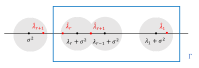
Figure 1: The contour plot of $\Gamma$. All grey balls share the same radius $\|\Delta\|$.

By Cauchy’s integral formula,

$$\frac{1}{2\pi i}\oint_{\Gamma}(\eta I-\hat{\Sigma})^{-1}d\eta$$

$$=\sum_{i=1}^{r}\frac{1}{2\pi i}\oint_{\Gamma}\frac{d\eta}{\eta-\hat{\lambda}_{i}}(\widehat{u}_{i}\widehat{u}_{i}^{\top})+\sum_{i=r+1}^{p}\frac{1}{2\pi i}\oint_{\Gamma}\frac{d\eta}{\eta-\hat{\lambda}_{i}}(\widehat{u}_{i}\widehat{u}_{i}^{\top})$$

$$=\sum_{i=1}^{r}\widehat{u}_{i}\widehat{u}_{i}^{\top}=\widehat{U}\widehat{U}^{\top}.$$

As a result, we have

$$\widehat{U}\widehat{U}^{\top}=\frac{1}{2\pi i}\oint_{\Gamma}(\eta I-\hat{\Sigma})^{-1}d\eta,$$ (27)

and similarly,

$$UU^{\top}=\frac{1}{2\pi i}\oint_{\Gamma}(\eta I-\Sigma)^{-1}d\eta.$$ (28)

We denote $\mathcal{R}_{\Sigma}(\eta):=(\eta I-\Sigma)^{-1}$ and thus

$$(\eta I-\hat{\Sigma})^{-1}=(\eta I-\Sigma-\Delta)^{-1}= \big{[}(\eta I-\Sigma)\big{(}I-\mathcal{R}_{\Sigma}(\eta)\Delta\big{)}\big{]}^{-1}$$

$$= \big{(}I-\mathcal{R}_{\Sigma}(\eta)\Delta\big{)}^{-1}\mathcal{R}_{\Sigma}(\eta).$$

Since

$$\big{\|}\mathcal{R}_{\Sigma}(\eta)\Delta\big{\|}\leq\|\mathcal{R}_{\Sigma}(\eta)\|\|\Delta\|\leq\frac{2\|\Delta\|}{\tilde{\lambda}_{r}}<1.$$

the Neumann series of $\big{(}I-\mathcal{R}_{\Sigma}(\eta)\Delta\big{)}^{-1}$ is

$$\big{(}I-\mathcal{R}_{\Sigma}(\eta)\Delta\big{)}^{-1}=I+\sum_{k\geq 1}[\mathcal{R}_{\Sigma}(\eta)\Delta]^{k}.$$ (29)

Plugging (29) and $\mathcal{R}_{\Sigma}(\eta)=(\eta I-\Sigma)^{-1}$ into (27), we have

$$\widehat{U}\widehat{U}^{\top}= \frac{1}{2\pi i}\oint_{\Gamma}(\eta I-\hat{\Sigma})^{-1}d\eta$$

$$= \frac{1}{2\pi i}\oint_{\Gamma}\mathcal{R}_{\Sigma}(\eta)d\eta+\sum_{k\geq 1}\frac{1}{2\pi i}\oint_{\Gamma}\big{[}\mathcal{R}_{\Sigma}(\eta)\Delta\big{]}^{k}\mathcal{R}_{\Sigma}(\eta)d\eta$$

$$= UU^{\top}+\sum_{k\geq 1}\frac{1}{2\pi i}\oint_{\Gamma}\big{[}\mathcal{R}_{\Sigma}(\eta)\Delta\big{]}^{k}\mathcal{R}_{\Sigma}(\eta)d\eta.$$

Then we can write

$$\widehat{U}\widehat{U}^{\top}-UU^{\top}=\sum_{k\geq 1}\frac{1}{2\pi i}\oint_{\Gamma}\big{[}\mathcal{R}_{\Sigma}(\eta)\Delta\big{]}^{k}\mathcal{R}_{\Sigma}(\eta)d\eta.$$

We denote the $k$-th order perturbation as

$$\mathcal{S}_{\Sigma,k}(\Delta):=\frac{1}{2\pi i}\oint_{\Gamma}\big{[}\mathcal{R}_{\Sigma}(\eta)\Delta\big{]}^{k}\mathcal{R}_{\Sigma}(\eta)d\eta$$ (30)

for all integer $k\geq 1$ and hence obtain

$$\widehat{U}\widehat{U}^{\top}-UU^{\top}=\sum_{k\geq 1}\mathcal{S}_{\Sigma,k}(\Delta).$$ (31)

We derive the explicit formulas for $\mathcal{S}_{\Sigma,1}(\Delta)$ and $\mathcal{S}_{\Sigma,2}(\Delta)$ as an appetizer served before showing the explicit formulas for $\mathcal{S}_{\Sigma,k}(\Delta)$ with general integer $k\geq 1$. Note that

$$\mathcal{R}_{\Sigma}(\eta)=\sum_{j=1}^{p}\frac{1}{\eta-\tilde{\lambda}_{j}}u_{j}u_{j}^{\top},$$

where $\tilde{\lambda}_{i}=\lambda_{i}+\sigma^{2}$ for $i\in[r]$ and $\tilde{\lambda}_{i}=\sigma^{2}$, for $i\in[p]\setminus[r]$. Let $P_{j}=u_{j}u_{j}^{\top}$ be the spectral projector onto $u_{j}$, for all $j\in[p]$.

Derivation of $\mathcal{S}_{\Sigma,1}(\Delta)$.

By the definition of $\mathcal{S}_{\Sigma,1}(\Delta)$,

$$\mathcal{S}_{\Sigma,1}(\Delta)= \frac{1}{2\pi i}\oint_{\Gamma}\mathcal{R}_{\Sigma}(\eta)\Delta\mathcal{R}_{\Sigma}(\eta)d\eta$$

$$= \sum_{j_{1}=1}^{p}\sum_{j_{2}=1}^{p}\frac{1}{2\pi i}\oint_{\Gamma}\frac{d\eta}{(\eta-\tilde{\lambda}_{j_{1}})(\eta-\tilde{\lambda}_{j_{2}})}P_{j_{1}}\Delta P_{j_{2}}.$$ (32)

Case 1: When both $j_{1}$ and $j_{2}$ are greater than $r$, the contour integral in (32) is zero according to Cauchy’s integral formula.
Case 2: When only one of $j_{1}$ and $j_{2}$ is greater than $r$. W.L.O.G, we assume $j_{2}>r$, then

$$\sum_{j_{1}=1}^{r}\sum_{j_{2}>r}^{p}\frac{1}{2\pi i}\oint_{\Gamma}\frac{d\eta}{(\eta-\tilde{\lambda}_{j_{1}})(\eta-\tilde{\lambda}_{j_{2}})}P_{j_{1}}\Delta P_{j_{2}}$$

$$=\sum_{j_{1}=1}^{r}\sum_{j_{2}>r}(\tilde{\lambda}_{j_{1}}-\tilde{\lambda}_{j_{2}})^{-1}P_{j_{1}}\Delta P_{j_{2}}$$

$$=\sum_{j_{1}=1}^{r}\sum_{j_{2}>r}(\lambda_{j_{1}})^{-1}P_{j_{1}}\Delta P_{j_{2}}$$

$$=Q^{-1}\Delta Q^{\perp},$$

where and $Q^{-1}=U\Lambda^{-1}U^{\top}$ and $Q^{\perp}=U_{\perp}U_{\perp}^{\top}$.
Case 3: When none of $j_{1}$ or $j_{2}$ is greater than $r$, the contour integral in (32) is zero.

In summary, $\mathcal{S}_{\Sigma,1}(\Delta)=Q^{-1}\Delta Q^{\perp}+Q^{\perp}\Delta Q^{-1}$.

Derivation of $\mathcal{S}_{\Sigma,2}(\Delta)$.

By the definition of $\mathcal{S}_{\Sigma,2}(\Delta)$,

$$\mathcal{S}_{\Sigma,2}(\Delta)= \frac{1}{2\pi i}\oint_{\Gamma}\mathcal{R}_{\Sigma}(\eta)\Delta\mathcal{R}_{\Sigma}(\eta)\Delta\mathcal{R}_{\Sigma}(\eta)d\eta$$

$$= \sum_{j_{1}=1}^{p}\sum_{j_{2}=1}^{p}\sum_{j_{3}=1}^{p}\frac{1}{2\pi i}\oint_{\Gamma}\frac{d\eta}{(\eta-\tilde{\lambda}_{j_{1}})(\eta-\tilde{\lambda}_{j_{2}})(\eta-\tilde{\lambda}_{j_{3}})}P_{j_{1}}\Delta P_{j_{2}}\Delta P_{j_{3}}.$$ (33)

Case 1: When all $j_{1},j_{2},j_{3}$ are greater than $r$, the contour integral in (33) is zero by Cauchy’s integral formula.
Case 2: When two of $j_{1},j_{2},j_{3}$ are greater than $r$. W.L.O.G., we assume $j_{1}\leq r$ and $j_{2},j_{3}>r$, then

$$\sum_{j_{1}=1}^{r}\sum_{j_{2},j_{3}>r}^{p}\frac{1}{2\pi i}\oint_{\Gamma}\frac{d\eta}{(\eta-\tilde{\lambda}_{j_{1}})(\eta-\tilde{\lambda}_{j_{2}})(\eta-\tilde{\lambda}_{j_{3}})}P_{j_{1}}\Delta P_{j_{2}}\Delta P_{j_{3}}$$

$$= \sum_{j_{1}=1}^{r}\sum_{j_{2},j_{3}>r}^{p}\frac{1}{(\tilde{\lambda}_{j_{1}}-\tilde{\lambda}_{j_{2}})(\tilde{\lambda}_{j_{1}}-\tilde{\lambda}_{j_{3}})}P_{j_{1}}\Delta P_{j_{2}}\Delta P_{j_{3}}=Q^{-2}\Delta Q^{\perp}\Delta Q^{\perp}$$

$$= \sum_{j_{1}=1}^{r}\sum_{j_{2},j_{3}>r}^{p}\frac{1}{\lambda_{j_{1}}^{2}}P_{j_{1}}\Delta P_{j_{2}}\Delta P_{j_{3}}=Q^{-2}\Delta Q^{\perp}\Delta Q^{\perp}.$$

Case 3: one of $j_{1},j_{2},j_{3}$ is greater than $r$. W.L.O.G., let $j_{1},j_{2}\leq r$ and $j_{3}>r$, we get

$$\sum_{j_{1},j_{2}=1}^{r}\sum_{j_{3}>r}^{p}\frac{1}{2\pi i}\oint_{\Gamma}\frac{d\eta}{(\eta-\tilde{\lambda}_{j_{1}})(\eta-\tilde{\lambda}_{j_{2}})(\eta-\tilde{\lambda}_{j_{3}})}P_{j_{1}}\Delta P_{j_{2}}\Delta P_{j_{3}}$$

$$= \sum_{j_{1}=j_{2}=1}^{r}\sum_{j_{3}>r}^{p}\frac{1}{2\pi i}\oint_{\Gamma}\frac{d\eta}{(\eta-\tilde{\lambda}_{j_{1}})^{2}(\eta-\tilde{\lambda}_{j_{3}})}P_{j_{1}}\Delta P_{j_{1}}\Delta P_{j_{3}}$$

$$\quad+\sum_{j_{1}\neq j_{2}\geq 1}^{r}\sum_{j_{3}>r}^{p}\frac{1}{2\pi i}\oint_{\Gamma}\frac{d\eta}{(\eta-\tilde{\lambda}_{j_{1}})(\eta-\tilde{\lambda}_{j_{2}})(\eta-\tilde{\lambda}_{j_{3}})}P_{j_{1}}\Delta P_{j_{2}}\Delta P_{j_{3}}$$

$$= -\sum_{j_{1}=1}^{r}(\tilde{\lambda}_{j_{1}}-\tilde{\lambda}_{j_{3}})^{-2}P_{j_{1}}\Delta P_{j_{1}}\Delta Q^{\perp}-\sum_{j_{1}\neq j_{2}\geq 1}^{r}(\tilde{\lambda}_{j_{1}}-\tilde{\lambda}_{j_{3}})^{-1}(\tilde{\lambda}_{j_{2}}-\tilde{\lambda}_{j_{3}})^{-1}P_{j_{1}}\Delta P_{j_{2}}\Delta Q^{\perp}$$

$$= -\sum_{j_{1}=1}^{r}\lambda_{j_{1}}^{-2}P_{j_{1}}\Delta P_{j_{1}}\Delta Q^{\perp}-\sum_{j_{1}\neq j_{2}\geq 1}^{r}\lambda_{j_{1}}^{-1}\lambda_{j_{2}}^{-1}P_{j_{1}}\Delta P_{j_{2}}\Delta Q^{\perp}$$

$$= -Q^{-1}\Delta Q^{-1}\Delta Q^{\perp}.$$

Case 4: When none of $j_{1},j_{2},j_{3}$ is greater than $r$, the contour integral in (33) is zero.

In summary,

$$\mathcal{S}_{\Sigma,2}(\Delta)= \big{(}Q^{-2}\Delta Q^{\perp}\Delta Q^{\perp}+Q^{\perp}\Delta Q^{-2}\Delta Q^{\perp}+Q^{\perp}\Delta Q^{\perp}\Delta Q^{-2}\big{)}$$

$$- \big{(}Q^{\perp}\Delta Q^{-1}\Delta Q^{-1}+Q^{-1}\Delta Q^{\perp}\Delta Q^{-1}+Q^{-1}\Delta Q^{-1}\Delta Q^{\perp}\big{)}.$$

Derivation of $\mathcal{S}_{\Sigma,k}(\Delta)$ for general k.

By the definition of $\mathcal{S}_{\Sigma,k}(\Delta)$,

$$\mathcal{S}_{\Sigma,k}(\Delta)=\sum_{j_{1},\cdots,j_{k+1}\geq 1}^{p}\frac{1}{2\pi i}\oint_{\Gamma}\Big{(}\prod_{i=1}^{k+1}\frac{1}{\eta-\tilde{\lambda}_{j_{i}}}\Big{)}d\eta P_{j_{1}}\Delta P_{j_{2}}\Delta\cdots P_{j_{k}}\Delta P_{j_{k+1}}.$$ (34)

In order to deal with each component in the summations (34), we first consider some special cases for ease of the notation. W.L.O.G., we consider the cases where some $\bar{k}$ indices from $\{j_{1},\cdots,j_{k+1}\}$ are not larger than $r$. More specifically, we restrict our discussion to the case where $j_{1},\cdots,j_{\bar{k}}\leq r$ and $j_{\bar{k}+1},\cdots,j_{k+1}>r$. By Cauchy integral formula, the integral in (34) is zero once $\bar{k}=0$ or $\bar{k}=k+1$ and thus we focus on the non-trivial case $\bar{k}\in[k-1]$. Note that

$$\sum_{j_{1},\cdots,j_{\bar{k}}\geq 1}^{r}\sum_{j_{\bar{k}+1},\cdots,j_{k+1}>r}^{p}\frac{1}{2\pi i}\oint_{\Gamma}\Big{(}\prod_{i=1}^{p}\frac{1}{\eta-\tilde{\lambda}_{j_{i}}}\Big{)}d\eta P_{j_{1}}\Delta P_{j_{2}}\Delta\cdots P_{j_{k}}\Delta P_{j_{k+1}}$$

$$=\sum_{j_{1},\cdots,j_{\bar{k}}\geq 1}^{r}\sum_{j_{\bar{k}+1},\cdots,j_{k+1}>r}^{p}\frac{1}{2\pi i}\oint_{\Gamma}\Big{(}\prod_{i=1}^{\bar{k}}\frac{1}{\eta-(\lambda_{j_{i}}+\sigma^{2})}\Big{)}(\eta-\sigma^{2})^{\bar{k}-k-1}d\eta P_{j_{1}}\Delta P_{j_{2}}\Delta\cdots P_{j_{k}}\Delta P_{j_{k+1}}$$

$$=\sum_{j_{1},\cdots,j_{\bar{k}}\geq 1}^{r}\frac{1}{2\pi i}\oint_{\Gamma}\Big{(}\prod_{i=1}^{\bar{k}}\frac{1}{\eta-(\lambda_{j_{i}}+\sigma^{2})}\Big{)}(\eta-\sigma^{2})^{\bar{k}-k-1}d\eta P_{j_{1}}\Delta P_{j_{2}}\Delta\cdots P_{j_{\bar{k}}}\Delta Q^{\perp}\Delta\cdots\Delta Q^{\perp}.$$

Recall that our goal is to prove

$$\mathcal{S}_{\Sigma,k}(\Delta)=\sum_{\mathbf{s}:s_{1}+\cdots+s_{k+1}=k}(-1)^{1+\tau(\mathbf{s})}\cdot Q^{-s_{1}}\Delta Q^{-s_{2}}\Delta\cdots\Delta Q^{-s_{k+1}}.$$

Accordingly, in the above summations, we consider the components, where $s_{1},\cdots,s_{\bar{k}}\geq 1$ and $s_{\bar{k}+1}=\cdots=s_{k+1}=0$, namely,

$$\sum_{\begin{subarray}{c}s_{1}+\cdots+s_{\bar{k}}=k\\ s_{j}\geq 1\end{subarray}}(-1)^{\bar{k}+1}Q^{-s_{1}}\Delta\cdots\Delta Q^{-s_{\bar{k}}}\Delta Q^{\perp}\cdots\Delta Q^{\perp}.$$

It turns out that we need to prove

$$\sum_{j_{1},\cdots,j_{\bar{k}}\geq 1}^{r}\frac{1}{2\pi i}\oint_{\Gamma}\Big{(}\prod_{i=1}^{\bar{k}}\frac{1}{\eta-(\lambda_{j_{i}}+\sigma^{2})}\Big{)}(\eta-\sigma^{2})^{\bar{k}-k-1}d\eta P_{j_{1}}\Delta P_{j_{2}}\Delta\cdots P_{j_{\bar{k}}}$$

$$=\sum_{j_{1},\cdots,j_{\bar{k}}\geq 1}^{r}\sum_{\begin{subarray}{c}s_{1}+\cdots+s_{\bar{k}}=k\\ s_{j}\geq 1\end{subarray}}(-1)^{\bar{k}+1}\frac{1}{(\lambda_{j_{1}})^{s_{1}}\cdots(\lambda_{j_{\bar{k}}})^{s_{\bar{k}}}}P_{j_{1}}\Delta P_{j_{2}}\Delta\cdots\Delta P_{j_{\bar{k}}}.$$

It suffices to prove that for all $\mathbf{j}=(j_{1},\dots,j_{\bar{k}})\in\{1,\cdots,r\}^{\bar{k}}$,

$$\frac{1}{2\pi i}\oint_{\Gamma}\Big{(}\prod_{i=1}^{\bar{k}}\frac{1}{\eta-(\lambda_{j_{i}}+\sigma^{2})}\Big{)}(\eta-\sigma^{2})^{\bar{k}-k-1}d\eta$$ (35)

$$=\sum_{\begin{subarray}{c}s_{1}+\cdots+s_{\bar{k}}=k\\ s_{j}\geq 1\end{subarray}}(-1)^{\bar{k}+1}\frac{1}{(\lambda_{j_{1}})^{s_{1}}\cdots(\lambda_{j_{\bar{k}}})^{s_{\bar{k}}}}.$$

To prove (35), we rewrite its right hand side. Given any $\mathbf{j}=(j_{1},\cdots,j_{\bar{k}})\in\{1,\cdots,r\}^{\bar{k}}$, we define

$$V_{i}(\mathbf{j}):=\big{\{}1\leq t\leq\bar{k}:j_{t}=i\big{\}}\quad\forall i\in[r],$$

as a set that contains all location $l\in[k+1]$ such that $\lambda_{j_{l}}=\lambda_{i}$. For simplicity, we also denote $v_{i}(\mathbf{j})=\left|V_{i}(\mathbf{j})\right|$. Then, the right hand side of (35) is written as

$$\sum_{\begin{subarray}{c}s_{1}+\cdots+s_{\bar{k}}=k\\ s_{j}\geq 1\end{subarray}}(-1)^{\bar{k}+1}\frac{1}{(\lambda_{j_{1}})^{s_{1}}\cdots(\lambda_{j_{\bar{k}}})^{s_{\bar{k}}}}$$

$$=(-1)^{\bar{k}+1}\sum_{\begin{subarray}{c}s_{1}+\cdots+s_{\bar{k}}=k\\ s_{j}\geq 1\end{subarray}}\lambda_{1}^{-\sum_{p\in V_{1}(\mathbf{j})}s_{p}}\cdots\lambda_{r}^{-\sum_{p\in V_{r}(\mathbf{j})}s_{p}}.$$

Now, we denote $t_{i}(\mathbf{j})=\sum_{p\in V_{i}(\mathbf{j})}s_{p}$ for all $i\in[r]$ and rewrite the above equation as

$$\sum_{\begin{subarray}{c}s_{1}+\cdots+s_{\bar{k}}=k\\ s_{j}\geq 1\end{subarray}}(-1)^{\bar{k}+1}\frac{1}{\lambda_{j_{1}}^{s_{1}}\cdots\lambda_{j_{\bar{k}}}^{s_{\bar{k}}}}$$

$$=(-1)^{\bar{k}+1}\sum_{\begin{subarray}{c}t_{1}(\mathbf{j})+\cdots+t_{r}(\mathbf{j})=k\\ t_{i}(\mathbf{j})\geq v_{i}(\mathbf{j})\\ t_{i}(\mathbf{j})=0\ {\rm if}\ v_{i}(\mathbf{j})=0\end{subarray}}\prod_{i:v_{i}(\mathbf{j})\geq 1}{\binom{t_{i}(\mathbf{j})-1}{v_{i}(\mathbf{j})-1}}\lambda_{i}^{-t_{i}(\mathbf{j})}$$

$$=(-1)^{\bar{k}+1}\sum_{\begin{subarray}{c}t_{1}(\mathbf{j})+\cdots+t_{r}(\mathbf{j})\\ =k-\bar{k}\\ t_{i}(\mathbf{j})=0\;\text{if}\;v_{i}(\mathbf{j})=0\end{subarray}}\prod_{i:v_{i}(\mathbf{j})\geq 1}{\binom{t_{i}(\mathbf{j})+v_{i}(\mathbf{j})-1}{v_{i}(\mathbf{j})-1}\lambda_{i}^{-t_{i}(\mathbf{j})-v_{i}(\mathbf{j})}}$$

where the last equality is due to the fact $v_{1}(\mathbf{j})+\cdots+v_{r}(\mathbf{j})=\bar{k}$. Similarly, the left hand side of (35) can be written as

$$\frac{1}{2\pi i}\oint_{\Gamma}\frac{d\eta}{(\eta-(\lambda_{j_{1}}+\sigma^{2}))\cdots(\eta-(\lambda_{j_{\bar{k}}}+\sigma^{2}))(\eta-\sigma^{2})^{k+1-\bar{k}}}$$

$$=\frac{1}{2\pi i}\oint_{\Gamma}\frac{d\eta}{(\eta-(\lambda_{1}+\sigma^{2}))^{v_{1}(\mathbf{j})}\cdots(\eta-(\lambda_{r}+\sigma^{2}))^{v_{r}(\mathbf{j})}(\eta-\sigma^{2})^{k+1-\bar{k}}}.$$

Therefore, in order to prove (35), it suffices to prove that for any $\mathbf{j}=(j_{1},\cdots,j_{\bar{k}})$ the following equality holds

$$\frac{1}{2\pi i}\oint_{\Gamma}\frac{d\eta}{(\eta-(\lambda_{1}+\sigma^{2}))^{v_{1}}\cdots(\eta-(\lambda_{r}+\sigma^{2}))^{v_{r}}(\eta-\sigma^{2})^{k+1-\bar{k}}}$$ (36)

$$=(-1)^{\bar{k}+1}\sum_{\begin{subarray}{c}t_{1}+\cdots+t_{r}=k-\bar{k}\\ t_{i}=0\ {\rm if}\ v_{i}=0\end{subarray}}\prod_{i:v_{i}\geq 1}^{r}{\binom{t_{i}+v_{i}-1}{v_{i}-1}}\lambda_{i}^{-t_{i}-v_{i}},$$

where we omitted the index $\mathbf{j}$ in definitions of $v_{i}(\mathbf{j})$ and $t_{i}(\mathbf{j})$ without causing any confusions. The non-negative numbers $v_{1}+\cdots+v_{r}=\bar{k}$. Let

$$\varphi(\eta)=\frac{1}{(\eta-(\lambda_{1}+\sigma^{2}))^{v_{1}}\cdots(\eta-(\lambda_{r}+\sigma^{2}))^{v_{r}}(\eta-\sigma^{2})^{k+1-\bar{k}}},$$

be a function of $\eta$. According to the Residue theorem,

$$\frac{1}{2\pi i}\oint_{\Gamma}\varphi(\eta)d\eta=-{\rm Res}(\varphi,\eta=\infty)-{\rm Res}(\varphi,\eta=\sigma^{2}).$$

Note that ${\rm Res}(\varphi,\eta=\infty)=0$ and it suffices to calculate ${\rm Res}(\varphi,\eta=\sigma^{2})$. Let $\gamma_{\sigma^{2}}$ be a contour plot around $\eta=\sigma^{2}$ such that none of $\{\lambda_{i}+\sigma^{2}\}_{i\in[r]}$ lies in $\partial\gamma_{\sigma^{2}}$. Then,

$${\rm Res}(\varphi,\eta=\sigma^{2})=\frac{1}{2\pi i}\oint_{\gamma_{\sigma^{2}}}\varphi(\eta)d\eta.$$

By Cauchy integral formula for derivatives, we have

$${\rm Res}(\varphi,\eta=\sigma^{2})$$

$$=\varphi^{(k-\bar{k})}(\eta)\Big{|}_{\eta=\sigma^{2}}$$

$$=\frac{1}{(k-\bar{k})!}\Big{[}\prod_{i:v_{i}\geq 1}^{r}(\eta-(\lambda_{i}+\sigma^{2}))^{-v_{i}}\Big{]}^{(k-\bar{k})}\Big{|}_{\eta=\sigma^{2}}$$

where $\varphi(\eta)^{(k-\bar{k})}$ is the $k-\bar{k}$-th order differentiation of $\varphi(\eta)$. Further, by general Leibniz rule,

$${\rm Res}(\varphi,\eta=0)$$

$$=\frac{1}{(k-\bar{k})!}\sum_{\begin{subarray}{c}t_{1}+\cdots+t_{r}=k-\bar{k}\\ t_{i}=0\ {\rm if}\ v_{i}=0\end{subarray}}\frac{(k-\bar{k})!}{t_{1}!t_{2}!\cdots t_{r}!}\prod_{i:v_{i}\geq 1}^{r}\Big{[}(\eta-(\lambda_{i}+\sigma^{2})^{-v_{i}}\Big{]}^{(t_{i})}\Big{|}_{\eta=\sigma^{2}}$$

$$=(-1)^{k-\bar{k}}\sum_{\begin{subarray}{c}t_{1}+\cdots+t_{r}=k-\bar{k}\\ t_{i}=0\ {\rm if}\ v_{i}=0\end{subarray}}\prod_{i:v_{i}\geq 1}^{r}\frac{v_{i}(v_{i}+1)\cdots(v_{i}+t_{i}-1)}{t_{i}!}(-\lambda_{i})^{-v_{i}-t_{i}}$$

$$=(-1)^{k-\bar{k}}\sum_{\begin{subarray}{c}t_{1}+\cdots+t_{r}=k-\bar{k}\\ t_{i}=0\ {\rm if}\ v_{i}=0\end{subarray}}\prod_{i:v_{i}\geq 1}^{r}{\binom{t_{i}+v_{i}-1}{v_{i}-1}}(-\lambda_{i})^{-v_{i}-t_{i}}$$

$$=(-1)^{2k-\bar{k}}\sum_{\begin{subarray}{c}t_{1}+\cdots+t_{r}=k-\bar{k}\\ t_{i}=0\ {\rm if}\ v_{i}=0\end{subarray}}\prod_{i:v_{i}\geq 1}^{r}{\binom{t_{i}+v_{i}-1}{v_{i}-1}}(\lambda_{i})^{-v_{i}-t_{i}}.$$

Therefore,

$$\frac{1}{2\pi i}\oint_{\Gamma}\varphi(\eta)d\eta=(-1)^{\bar{k}+1}\sum_{\begin{subarray}{c}t_{1}+\cdots+t_{r}=k-\bar{k}\\ t_{i}=0\ {\rm if}\ v_{i}=0\end{subarray}}\prod_{i:v_{i}\geq 1}^{r}{\binom{t_{i}+v_{i}-1}{v_{i}-1}}\lambda_{i}^{-v_{i}-t_{i}}$$

which shows (LABEL:aim) is true and the proof is completed.

A.3 Proof of Lemma 6

Recall that the Kullback-Leibler divergence and total variation distance between two probability measures defined in the same measure space $(\Omega,\mathcal{F})$ are defined by

$${\rm TV}(\mu\|\nu):=\int_{\Omega}\log\left(\frac{\mu(dx)}{\nu(dx)}\right)\mu(dx)\quad{\rm and}\quad{\rm TV}(\mu,\nu):=\sup_{E\in\mathcal{F}}|\mu(E)-\nu(E)|.$$

By definition, for any $(\varepsilon,0)$-DP algorithm $A$, we have

$$\sup_{P\in\mathcal{P}}\mathbb{E}_{A}\;\rho(A,\theta(P)) \geq\sup_{P\in\mathcal{Q}}\mathbb{E}_{A}\;\rho(A,\theta(P))$$

$$\geq\frac{1}{N}\sum_{i=1}^{N}\frac{\rho_{0}}{2}\mathbb{E}_{A}\mathbb{I}\left(\rho\left(A,\theta(P_{i})\right)>\frac{\rho_{0}}{2}\right).$$

Following the proof of generalized Fano’s Lemma (Devroye, 1987; Yu, 1997), we further reduce the estimation problem into hypothesis testing. Let $h:\Theta\rightarrow\Theta_{\mathcal{Q}}$ be defined by $h(\theta)=\underset{\theta_{i}\in\Theta_{\mathcal{Q}}}{\operatorname{argmin}}\;\rho\left(\theta_{i},\theta\right)$. For all $i,j\in[N]$, define

$$p_{ji}:=\mathbb{E}_{A,X\sim P_{j}}\mathbb{I}(h(A)=\theta(P_{i})),$$

measuring the probability that the algorithm $A$ outputs an estimator closer to $\theta(P_{i})$ using data actually sampled from distribution $P_{j}$. The total type-I error of testing $H_{0}:X\sim P_{j}$ versus $H_{1}:X\sim P\in\mathcal{P}\setminus P_{j}$ is

$$\beta_{j}:=\mathbb{E}_{A,X\sim P_{j}}\mathbb{I}(h(A)\neq\theta(P_{j}))=\sum_{i\neq j}p_{ji}.$$

Observe that

$$\frac{1}{N}\sum_{i=1}^{N}\frac{\rho_{0}}{2}\mathbb{E}_{A}\mathbb{I}\left(\rho\left(A,\theta(P_{i})\right)>\frac{\rho_{0}}{2}\right)\geqslant\frac{\rho_{0}}{2N}\sum_{i=1}^{N}\mathbb{E}_{A,X\sim P_{i}}\mathbb{I}(h\left(A\right)\neq\theta(P_{i}))=\frac{\rho_{0}}{2N}\sum_{i=1}^{N}\beta_{i}.$$

Therefore,

$$\sup_{P\in\mathcal{P}}\mathbb{E}_{A}\;\rho(A,\theta(P))\geq\frac{\rho_{0}}{2N}\sum_{i=1}^{N}\beta_{i}.$$

It suffices to find a lower bound for $\sum_{i=1}^{N}\beta_{i}$. Towards that end, the following lemma is needed. Its proof is relegated to Section B.4

Lemma 13.

Let $\mu=\mu_{1}\times\cdots\times\mu_{n}$ and $\nu=\nu_{1}\times\cdots\times\nu_{n}$ be two probability measures defined on the same measurable space $(\Omega,\mathcal{F})$. The total variation distance is denoted by $t_{k}=\operatorname{\operatorname{TV}}(\mu_{k},\nu_{k})$ for all $k\in[n]$. Let $A:\Omega\mapsto\Theta$ be an $(\varepsilon,\delta)$-DP random algorithm. Then, for any subset $E\subset\Theta$,

$$\mathbb{E}_{A,X\sim\mu}\mathbb{I}\big{(}A(X)\in E\big{)} \leq\exp\bigg{(}4\varepsilon\sum_{k=1}^{n}t_{k}\bigg{)}\left(\mathbb{E}_{A,X\sim\nu}\mathbb{I}\big{(}A(X)\in E\big{)}+\frac{2\delta}{e^{\varepsilon}-1}\right),$$

Now consider any pair $P_{i},P_{j}\in\mathcal{Q}$ where $P_{i}=\mu_{i}^{(1)}\times\cdots,\times\mu_{i}^{(n)}$ and $P_{j}=\mu_{j}^{(1)}\times\cdots,\times\mu_{j}^{(n)}$. By Lemma 13 and the fact $p_{ii}+\sum_{j\neq i}p_{ij}=1$ , we have

$$p_{ji} \geqslant\exp\left(-4\varepsilon\sum_{k\in[n]}\operatorname{TV}\left(\mu_{i}^{(k)},\mu_{j}^{(k)}\right)\right)p_{ii}-\frac{2\delta}{e^{\varepsilon}-1}$$

$$=\exp\left(-4\varepsilon\sum_{k\in[n]}\operatorname{TV}\left(\mu_{i}^{(k)},\mu_{j}^{(k)}\right)\right)\left(1-\sum_{j\neq i}p_{ij}\right)-\frac{2\delta}{e^{\varepsilon}-1}$$

$$=\exp\left(-4\varepsilon\sum_{k\in[n]}\operatorname{TV}\left(\mu_{i}^{(k)},\mu_{j}^{(k)}\right)\right)\left(1-\beta_{i}\right)-\frac{2\delta}{e^{\varepsilon}-1}$$

$$\geq\exp\left(-4\varepsilon t_{0}\right)\left(1-\beta_{i}\right)-\frac{2\delta}{e^{\varepsilon}-1}.$$

Taking summation over $i\in[N]\setminus\{j\}$, we have

$$\beta_{j}=\sum_{i\neq j}p_{ji}\geqslant\exp\left(-4\varepsilon t_{0}\right)\left(N-1-\sum_{i\neq j}\beta_{i}\right)-\frac{2(N-1)\delta}{e^{\varepsilon}-1}$$

Further summing over $j\in[N]$, we have

$$\sum_{j=1}^{N}\beta_{j}\geqslant\frac{N(N-1)}{(N-1)+\exp\left(4\varepsilon t_{0}\right)}\cdot\left(1-\frac{2\delta e^{4\varepsilon t_{0}}}{e^{\varepsilon}-1}\right).$$

Therefore,

$$\sup_{P\in\mathcal{P}}\mathbb{E}_{A}\;\rho(A,\theta(P)) \geq\frac{\rho_{0}}{2}\frac{(N-1)}{(N-1)+\exp\left(4\varepsilon t_{0}\right)}\cdot\left(1-\frac{2\delta e^{4\varepsilon t_{0}}}{e^{\varepsilon}-1}\right)$$

$$\geq\frac{\rho_{0}}{4}\left(1\wedge\frac{N-1}{\exp\left(4\varepsilon t_{0}\right)}\right)\left(1-\frac{2\delta e^{4\varepsilon t_{0}}}{e^{\varepsilon}-1}\right).$$

Combining the above lower bound with classical generalized Fano’s Lemma (e.g., Tsybakov (2008)), we have

$$\inf_{A\in\mathcal{A}_{\varepsilon,\delta}(\mathcal{P})} \sup_{P\in\mathcal{P}}\mathbb{E}_{A}\;\rho(A,\theta(P))\geqslant\max\left\{\frac{\rho_{0}}{2}\left(1-\frac{l_{0}+\log 2}{\log N}\right),\frac{\rho_{0}}{4}\left(1\wedge\frac{N-1}{\exp\left(4\varepsilon t_{0}\right)}\right)\left(1-\frac{2\delta e^{4\varepsilon t_{0}}}{e^{\varepsilon}-1}\right)\right\}.$$

A.4 Proof of Lemma 11

We begin with discussing the case $\mathbf{s}=(k,0,\cdots,0)$ and $l=1$. By definition, we have

$$\|\mathcal{T}_{\Sigma,k,\mathbf{s},1}\left(\Delta-\Delta^{(i)}\right)\|_{\rm F} =\|Q^{-k}\left(\Delta-\Delta^{(i)}\right)Q^{\perp}\Delta Q^{\perp}\cdots Q^{\perp}\Delta Q^{\perp}\|_{\rm F}$$

$$\leq\frac{1}{\lambda_{r}}\|U\left(\Delta-\Delta^{(i)}\right)U_{\perp}^{\top}\|_{\rm F}\left(\frac{\|\Delta\|}{\lambda_{r}}\right)^{k-1}.$$

By Lemma 9, in the event $\mathcal{E}^{\ast}$, we get

$$\|\mathcal{T}_{\Sigma,k,\mathbf{s},1}\left(\Delta-\Delta^{(i)}\right)\|_{\rm F}\lesssim\sqrt{\frac{\sigma^{2}(\lambda+\sigma^{2})}{\lambda^{2}}}\frac{\sqrt{p(r+\log n)}}{n}\left(\frac{D_{\max}}{\lambda_{r}}\right)^{k-3}.$$

For the cases $\mathbf{s}=(k,0,\cdots,0)$ and $2\leq l\leq k$,

$$\|\mathcal{T}_{\Sigma,k,\mathbf{s},l}\left(\Delta-\Delta^{(i)}\right)\|_{\rm F} =\|Q^{-k}\Delta^{(i)}Q^{\perp}\cdots Q^{\perp}\left(\Delta-\Delta^{(i)}\right)Q^{\perp}\cdots Q^{\perp}\Delta Q^{\perp}\|_{\rm F}$$

$$\leq\Big{\|}Q^{-k}\Delta^{(i)}Q^{\perp}\cdots Q^{\perp}\frac{1}{n}X_{i}X_{i}^{\top}Q^{\perp}\cdots Q^{\perp}\Delta Q^{\perp}\Big{\|}_{\rm F}$$

$$\quad+\Big{\|}Q^{-k}\Delta^{(i)}Q^{\perp}\cdots Q^{\perp}\frac{1}{n}X_{i}^{\prime}X_{i}^{\prime\top}Q^{\perp}\cdots Q^{\perp}\Delta Q^{\perp}\Big{\|}_{\rm F}.$$

We need to control each term in the RHS of above inequality. The proof of the following lemma can be found in the Appendix B.

Lemma 14.

For all $k\geq 2$ and $2\leq l\leq k$, the following bounds hold in the event $\mathcal{E}^{\ast}$.

$$\max_{i\in[n]}\Big{\|}Q^{-k}\Delta^{(i)}Q^{\perp}\cdots Q^{\perp} \frac{1}{n}X_{i}X_{i}^{\top}Q^{\perp}\cdots Q^{\perp}\Delta Q^{\perp}\Big{\|}_{\rm F}$$

$$\lesssim\left(\frac{D_{\max}}{\lambda_{r}}\right)^{k-2}\cdot\frac{\sigma^{2}}{\lambda}\sqrt{\frac{p}{n}}\cdot\sqrt{\frac{\sigma^{2}(\lambda+\sigma^{2})}{\lambda^{2}}}\frac{\sqrt{p(r+\log n)}}{n},$$

and moreover

$$\max_{i\in[n]}\Big{\|}Q^{-k}\Delta^{(i)}Q^{\perp}\cdots Q^{\perp}\frac{1}{n}X_{i}^{\prime}X_{i}^{\prime\top}Q^{\perp}\cdots Q^{\perp}\Delta Q^{\perp}\Big{\|}_{\rm F}$$

$$\lesssim l\left(\frac{D_{\max}}{\lambda_{r}}\right)^{k-2}\cdot\frac{\sigma^{2}}{\lambda}\Big{(}\sqrt{\frac{p}{n}}+\frac{p}{n}\Big{)}\cdot\sqrt{\frac{\sigma^{2}(\lambda+\sigma^{2})}{\lambda^{2}}}\frac{\sqrt{p(r+\log n)}}{n}.$$

Note that the $Q^{\perp}$ term appears $l-1$ times before $X_{i}X_{i}^{\top}$ or $X_{i}X_{i}^{\prime\top}$ in the above product sequences of matrices.

According to Lemma 14, for $2\leq l\leq k$

$$\|\mathcal{T}_{\Sigma,k,\mathbf{s},l}\left(\Delta-\Delta^{(i)}\right)\|_{\rm F}\lesssim(l+1)\left(\frac{D_{\max}}{\lambda_{r}}\right)^{k-2}\cdot\frac{\sigma^{2}}{\lambda}\Big{(}\sqrt{\frac{p}{n}}+\frac{p}{n}\Big{)}\cdot\sqrt{\frac{\sigma^{2}(\lambda+\sigma^{2})}{\lambda^{2}}}\frac{\sqrt{p(r+\log n)}}{n}.$$

Taking the summation over $l\in[k]$, we have

$$\sum_{l\in[k]}\|\mathcal{T}_{\Sigma,k,\mathbf{s},l}\left(\Delta-\Delta^{(i)}\right)\|_{\rm F} \lesssim\frac{(3+k)k}{2}\left(\frac{D_{\max}}{\lambda_{r}}\right)^{k-2}\cdot\frac{\sigma^{2}}{\lambda}\Big{(}\sqrt{\frac{p}{n}}+\frac{p}{n}\Big{)}\cdot\sqrt{\frac{\sigma^{2}(\lambda+\sigma^{2})}{\lambda^{2}}}\frac{\sqrt{p(r+\log n)}}{n},$$

which holds for $\mathbf{s}=\{k,0,\cdots,0\}$ and all $i\in[n]$.

We now argue that the above bound holds for all $\mathbf{s}:=\{s_{1},\cdots,s_{k+1}\}$ such that $\sum_{j}s_{j}=k$ and $s_{j}$’s are non-negative integers. For any $\mathbf{s}\in I_{k}\setminus\{k,0,\cdots,0\}$, there exists at least two subsequence within $\mathcal{T}_{\Sigma,k,\mathbf{s},l}\left(\Delta-\Delta^{(i)}\right)$ such that the sequence is starting from $UU^{\top}$ and ends with all other projectors being $U_{\perp}U_{\perp}^{\top}$ (Note that the other cases involving $U^{\top}(\Delta-\Delta^{(i)})U$ are smaller terms). Without loss of the generality, we discuss one subsequence where the first projector is $Q^{-\bar{k}}$ with $\bar{k}>0$ and the remaining projectors are all $Q_{\perp}$. Suppose that the target subsequence contains $t+1$ projectors $(t\leq k)$ with indices $(s_{m+1},\cdots,s_{m+t},s_{m+t+1})$ for some integer $m\geq 0$ satisfying $\sum_{j=m+1}^{m+t+1}s_{j}=\bar{k}$ and $\sum_{j=1}^{m}s_{j}+\sum_{j=m+t+2}^{j=k+1}s_{j}=k-\bar{k}$.

When $m+1\leq l\leq m+t+1$, the target subsequence times is upper bounded with the argument for the case $\mathbf{s}=(t,0,\cdots,0)$. The remaining part in $\mathcal{T}_{\Sigma,k,\mathbf{s},l}\left(\Delta-\Delta^{(i)}\right)$ contains $k-t$ projectors and is upper bounded by $D_{\max}^{k-t}/\lambda^{k-\bar{k}}$. Therefore,

$$\|\mathcal{T}_{\Sigma,k,\mathbf{s},l} \left(\Delta-\Delta^{(i)}\right)\|_{\rm F}$$

$$\lesssim\frac{D_{\max}^{k-t}}{\lambda^{k-\bar{k}}}\cdot\lambda^{t-\bar{k}}\cdot(l+1)\left(\frac{D_{\max}}{\lambda_{r}}\right)^{k-2}\cdot\frac{\sigma^{2}}{\lambda}\Big{(}\sqrt{\frac{p}{n}}+\frac{p}{n}\Big{)}\cdot\sqrt{\frac{\sigma^{2}(\lambda+\sigma^{2})}{\lambda^{2}}}\frac{\sqrt{p(r+\log n)}}{n}$$

$$\lesssim(l+1)\left(\frac{D_{\max}}{\lambda_{r}}\right)^{k-2}\cdot\frac{\sigma^{2}}{\lambda}\Big{(}\sqrt{\frac{p}{n}}+\frac{p}{n}\Big{)}\cdot\sqrt{\frac{\sigma^{2}(\lambda+\sigma^{2})}{\lambda^{2}}}\frac{\sqrt{p(r+\log n)}}{n}.$$

The same argument can be applied to the case $l\in[k+1]\setminus[m+1:m+t+1]$ and is skipped here. Finally we conclude that in event $\mathcal{E}^{\ast}$,

$$\sum_{l\in[k]}\|\mathcal{T}_{\Sigma,k,\mathbf{s},l}(\Delta-\Delta^{(i)})\|_{\rm F}\lesssim\frac{(3+k)k}{2}\left(\frac{D_{\max}}{\lambda_{r}}\right)^{k-2}\cdot\frac{\sigma^{2}}{\lambda}\Big{(}\sqrt{\frac{p}{n}}+\frac{p}{n}\Big{)}\cdot\sqrt{\frac{\sigma^{2}(\lambda+\sigma^{2})}{\lambda^{2}}}\frac{\sqrt{p(r+\log n)}}{n},$$

for $k\geq 2$ and any $\mathbf{s}\in I_{k}$. This concludes the proof of Lemma 11.

Appendix B Proofs of Technical Lemmas

B.1 Proof of Lemma 8

By the orthogonal invariance of normal distribution, we can simply assume $\Sigma={\rm diag}(\lambda_{1},\cdots,\lambda_{p})$ and as a result,

$$\|X\|^{2}\stackrel{{\scriptstyle{\rm d.}}}{{=}}\lambda_{1}Z_{1}^{2}+\cdots+\lambda_{p}Z_{p}^{2},$$

where $Z_{1},\cdots,Z_{p}$ are i.i.d. standard normal random variables. Note that $\lambda_{i}Z_{i}^{2}$ is sub-exponential ${\rm SE}(C_{1}\lambda_{i}^{2},C_{2}\lambda_{i})$ for some absolute constants $C_{1},C_{2}>0$ meaning that

$$\mathbb{P}\big{(}|\lambda_{i}Z_{i}^{2}-\lambda_{i}|\geq t\big{)}\leq\exp\bigg{(}-c_{1}\min\bigg{\{}\frac{t^{2}}{\lambda_{i}^{2}},\ \frac{t}{\lambda_{i}}\bigg{\}}\bigg{)},$$

for any $t>0$. By the composition property of sub-exponential random variables, we have

$$\lambda_{1}Z_{1}^{2}+\cdots+\lambda_{p}Z_{p}^{2}\in{\rm SE}\Big{(}C_{1}\sum_{i=1}^{p}\lambda_{i}^{2},C_{2}\lambda_{1}\Big{)}.$$

Therefore, we conclude that

$$\mathbb{P}\bigg{(}\Big{|}\|X\|^{2}-{\rm tr}(\Sigma)\Big{|}\leq C_{1}\Big{(}u\sum_{i=1}^{p}\lambda_{i}^{2}\Big{)}^{1/2}+C_{2}\lambda_{1}u\bigg{)}\geq 1-e^{-c_{1}u},$$

for any $u>0$. The proof of the upper bound $\|X_{i}\|^{2},\|U^{\top}X_{i}\|^{2}$ and $\|U_{\perp}^{\top}X_{i}\|^{2}$ is straightforward and skipped here.

B.2 Proof of Lemma 9

Recall that $\Delta=\widehat{\Sigma}-\Sigma$ and $\Delta^{(i)}=\widehat{\Sigma}^{(i)}-\Sigma$. By Lemma 7, we have

$$\mathbb{E}\|\Delta\|+\max_{i\in[n]}\|\Delta^{(i)}\|\leq C_{1}\Bigg{(}\sqrt{\frac{(\lambda+\sigma^{2})(r\lambda+p\sigma^{2})}{n}}+\frac{r\lambda+p\sigma^{2}}{n}\Bigg{)}\leq C_{2}\sqrt{\frac{(\lambda+\sigma^{2})(r\lambda+p\sigma^{2})}{n}},$$

where the last inequality is due to $C_{3}r\leq n$ and $\lambda/\sigma^{2}\geq C_{3}p/n$ for some large constant $C_{3}>0$. Since ${\rm tr}(\Sigma)\leq n\|\Sigma\|$, by Lemma 7, we get

$$\mathbb{P}\Bigg{(}\Big{|}\|\Delta\|-\mathbb{E}\|\Delta\|\Big{|}\leq C_{4}\sqrt{\frac{(\lambda+\sigma^{2})\big{(}r\lambda+p\sigma^{2}+t(\lambda+\sigma^{2})\big{)}}{n}}\Bigg{)}\geq 1-e^{-t}10^{-20\tilde{r}},$$

where $\tilde{r}$ denotes the effective rank ${\rm tr}(\Sigma)/\|\Sigma\|$. By choosing $t=0$, we conclude that

$$\mathbb{P}\bigg{(}\|\Delta\|\leq C_{4}\sqrt{\frac{(\lambda+\sigma^{2})(r\lambda+p\sigma^{2})}{n}}\bigg{)}\geq 1-10^{-20\tilde{r}}.$$

To bound $\|\Delta^{(i)}\|$, notice that $\Delta^{(i)}=\Delta-X_{i}X_{i}^{\top}/n+X_{i}^{\prime}X_{i}^{\prime\top}/n$ so that

$$\|\Delta^{(i)}\|\leq\|\Delta\|+\|X_{i}\|^{2}/n+\|X_{i}^{\prime}\|^{2}/n.$$

If $p\geq C_{5}\log n$ and $n\geq C_{5}\log^{2}n$, under the event $\mathcal{E}_{0}$ defined in Lemma 8, for some constant $C_{6}>0$

$$\max_{i\in[n]}\|\Delta^{(i)}\|\leq C_{6}\sqrt{\frac{(\lambda+\sigma^{2})(r\lambda+p\sigma^{2})}{n}}.$$

Therefore, there exists an event $\mathcal{E}_{\Delta}$ with probability $\mathbb{P}(\mathcal{E}_{\Delta})\geq 1-10^{-20\tilde{r}}-n^{-10}$ under which the following bound holds

$$\max_{i\in[n]}\|\Delta\|+\|\Delta^{(i)}\|\leq C_{6}\sqrt{\frac{(\lambda+\sigma^{2})(r\lambda+p\sigma^{2})}{n}}.$$

Now we study the bounds in event $\mathcal{E}_{1}$ and begin with $U^{\top}\Delta U_{\perp}$. By definition, we write

$$U^{\top}\Delta U_{\perp}=\frac{1}{n}\sum_{i=1}^{n}U^{\top}X_{i}X_{i}^{\top}U_{\perp}.$$

Since $X_{i}\sim\mathcal{N}(0,\Sigma)$ and by the spiked structure of $\Sigma$, we have

$$U^{\top}X_{i}\sim\mathcal{N}\big{(}0,\Lambda_{r}\big{)}\quad{\rm and}\quad U_{\perp}^{\top}X_{i}\sim\mathcal{N}\big{(}0,\sigma^{2}I_{p-r}\big{)},$$

where $\Lambda_{r}:={\rm diag}\big{(}\lambda_{1}+\sigma^{2},\cdots,\lambda_{r}+\sigma^{2}\big{)}$. Let $Z_{i}\sim\mathcal{N}(0,I_{r}),Y_{i}\sim\mathcal{N}(0,I_{p-r}),i\in[n]$ be independent Gaussian random vectors. Then

$$U^{\top}X_{i}\stackrel{{\scriptstyle{\rm d.}}}{{=}}\Lambda_{r}^{1/2}Z_{i}\quad{\rm and}\quad U_{\perp}^{\top}X_{i}\stackrel{{\scriptstyle{\rm d.}}}{{=}}\sigma Y_{i},\quad i\in[n].$$

As a result,

$$U^{\top}\Delta U_{\perp}\stackrel{{\scriptstyle{\rm d.}}}{{=}}\sigma\Lambda_{r}^{1/2}\frac{1}{n}\sum_{i=1}^{n}Z_{i}Y_{i}^{\top}\Longrightarrow\big{\|}U^{\top}\Delta U_{\perp}\big{\|}\leq\frac{\sqrt{\sigma^{2}(\lambda+\sigma^{2})}}{n}\Big{\|}\sum_{i=1}^{n}Z_{i}Y_{i}^{\top}\Big{\|}.$$

Denote $A:=[Z_{1},\cdots,Z_{n}]\in\mathbb{R}^{r\times n}$ and $B:=[Y_{1},\cdots,Y_{n}]^{\top}\in\mathbb{R}^{n\times(p-r)}$. Since $B\in\mathbb{R}^{n\times(p-r)}$ has i.i.d. $\mathcal{N}(0,1)$ entries, we are able to write $B=[\tilde{Y}_{1},\cdots,\tilde{Y}_{p-r}]$ with the column $\tilde{Y}_{i}$ i.i.d. to $\mathcal{N}(0,I_{p-r})$ for $i\in[p-r]$. We can therefore write $\sum_{i=1}^{n}Z_{i}Y_{i}^{\top}=AB$. Conditioned on $A$, the matrix

$$AB=\big{(}A\tilde{Y}_{1},\cdots,A\tilde{Y}_{p-r}\big{)},$$

has i.i.d. columns obeying the distribution $\mathcal{N}(0,AA^{\top})$. By Lemma 7,

$$\mathbb{P}\bigg{(}\|AA^{\top}/n-I_{r}\|\leq C_{3}\sqrt{\frac{rt}{n}}\bigg{)}\geq 1-e^{-t},$$

for any $t>0$. Therefore, if $n\geq C_{4}r\log n$, there exists an event $\mathcal{F}_{1}$ with $\mathbb{P}(\mathcal{F}_{1})\geq 1-n^{-10}$ under which the following bound holds

$$\frac{9n}{10}\leq\lambda_{\min}(AA^{\top})\leq\lambda_{\max}(AA^{\top})\leq\frac{11n}{10}.$$

Under the event $\mathcal{F}_{1}$, we apply Lemma 7 again and conclude with

$$\mathbb{P}\bigg{(}\Big{\|}\frac{ABB^{\top}A^{\top}}{p-r}-AA^{\top}\Big{\|}\leq\frac{n}{100}\bigg{)}\geq 1-e^{-c_{1}p},$$

where $c_{1}>0$ is a small constant and used the condition $p\geq 2r$. Finally, we conclude that

$$\mathbb{P}\Big{(}\|AB\|\leq C_{5}\sqrt{np}\Big{)}\geq 1-e^{-c_{1}p}-n^{-10}.$$

Therefore,

$$\big{\|}U^{\top}\Delta U_{\perp}\big{\|}\leq C_{5}\sqrt{\frac{p\sigma^{2}(\lambda+\sigma^{2})}{n}}.$$ (37)

To bound $\|U^{\top}\Delta^{(i)}U_{\perp}\|$, observe that

$$\big{\|}U^{\top}\Delta^{(i)}U_{\perp}\big{\|}\leq\big{\|}U^{\top}\Delta U_{\perp}\big{\|}+\|U^{\top}X_{i}\|\|U_{\perp}^{\top}X_{i}\|/n+\|U^{\top}X_{i}^{\prime}\|\|U_{\perp}^{\top}X_{i}\|/n.$$

Combining (37) and the event $\mathcal{E}_{0}$ defined in Lemma 8, we get

$$\mathbb{P}\bigg{(}\|U^{\top}\Delta U_{\perp}\|+\max_{i\in[n]}\|U^{\top}\Delta^{(i)}U_{\perp}\|\leq C_{5}\sqrt{\frac{p\sigma^{2}(\lambda+\sigma^{2})}{n}}\bigg{)}\geq 1-e^{-c_{1}p}-n^{-9},$$ (38)

where we used the fact $n\geq C_{1}(r+\log n)$.

Similarly, $U^{\top}X_{i}X_{i}^{\top}U_{\perp}\stackrel{{\scriptstyle{\rm d.}}}{{=}}\sigma\Lambda_{r}^{1/2}Z_{i}Y_{i}^{\top}$ so that $\|U^{\top}X_{i}X_{i}^{\top}U_{\perp}\|\leq C\sqrt{\sigma^{2}(\lambda+\sigma^{2})}\|Z_{i}\|\|Y_{i}\|$. Applying Lemma 8 again, we get

$$\mathbb{P}\Big{(}\max_{i\in[n]}\|U^{\top}X_{i}X_{i}^{\top}U_{\perp}\|+\|U^{\top}X_{i}^{\prime}X_{i}^{\prime\top}U_{\perp}\|\leq C_{5}\sqrt{\sigma^{2}(\lambda+\sigma^{2})p(r+\log n)}\Big{)}\geq 1-n^{-10}.$$ (39)

We now consider the last terms in the event $\mathcal{E}_{1}$. Note that $X_{i}$ is independent of $\sum_{j\neq i}X_{i}X_{j}^{\top}$. Conditioned on the latter one, we have

$$U^{\top}\Big{(}\frac{1}{n}\sum_{j\neq i}X_{j}X_{j}^{\top}\Big{)}U_{\perp}U_{\perp}^{\top}X_{i}\sim\mathcal{N}\bigg{(}0,\sigma^{2}U^{\top}\Big{(}\frac{1}{n}\sum_{j\neq i}X_{j}X_{j}^{\top}\Big{)}U_{\perp}U_{\perp}^{\top}\Big{(}\frac{1}{n}\sum_{j\neq i}X_{j}X_{j}^{\top}\Big{)}U\bigg{)}.$$

By the bound (38), we get

$$\Big{\|}U^{\top}\Big{(}\frac{1}{n}\sum_{j\neq i}X_{j}X_{j}^{\top}\Big{)}U_{\perp}\Big{\|}\leq C_{3}\sqrt{\frac{\sigma^{2}(\lambda+\sigma^{2})p}{n}},$$

which holds in event $\mathcal{E}_{\Delta}$. Now applying Lemma 8 where $u=C(r+\log n)$, we conclude that in event defined in (38),

$$\mathbb{P}\bigg{(}\Big{\|}U^{\top}\Big{(}\frac{1}{n}\sum_{j\neq i}X_{j}X_{j}^{\top}\Big{)}U_{\perp}U_{\perp}^{\top}X_{i}\Big{\|}\leq\sigma\cdot\sqrt{\frac{\sigma^{2}(\lambda+\sigma^{2})p(r+\log n)}{n}}\bigg{)}\geq 1-10^{-20r}n^{-10}.$$ (40)

By (38), (39), and (40), we conclude that $\mathbb{P}(\mathcal{E}_{1})\geq 1-e^{-c_{1}p}-2n^{-9}$.

B.3 Proof of Lemma 10

According to Lemma 5,

$$\widehat{U}\widehat{U}^{\top}-UU^{\top}=\sum_{k\geq 1}\mathcal{S}_{\Sigma,k}(\Delta).$$

For $k\geq 2$, there exists a term either of the form $Q^{-1}\Delta Q^{\perp}$ or $Q^{\perp}\Delta Q^{-1}$ in each summand of $\mathcal{S}_{\Sigma,k}(\Delta)$ and thus

$$\left\|\mathcal{S}_{\Sigma,k}(\Delta)\right\|\leq\binom{2k}{k}\left(\frac{\|\Delta\|}{\lambda_{r}}\right)^{k-1}\left\|Q^{-1}\Delta Q^{\perp}\right\|\leq\binom{2k}{k}\left(\frac{\|\Delta\|}{\lambda_{r}}\right)^{k-1}\frac{\left\|U^{\top}\Delta U_{\perp}\right\|}{\lambda_{r}},$$

where we use the fact

$$\left\|Q^{-1}\Delta Q^{\perp}\right\|=\left\|U\Lambda^{-1}U^{\top}\Delta U_{\perp}U_{\perp}^{\top}\right\|\leq\left(\lambda_{r}\right)^{-1}\left\|U^{\top}\Delta U_{\perp}\right\|.$$

For all integers $k\geq 1$, $\binom{2(k+1)}{k+1}\binom{2k}{k}^{-1}=2(2k+1)(k+1)^{-1}\leq 4$ and we have

$$\sum_{k=2}^{\infty}\left\|\mathcal{S}_{\Sigma,k}(\Delta)\right\| \leq\binom{4}{2}\frac{\|\Delta\|}{\lambda_{r}}\cdot\frac{\left\|U^{\top}\Delta U_{\perp}\right\|}{\lambda_{r}}\sum_{k=0}^{\infty}4^{k}\left(\frac{\|\Delta\|}{\lambda_{r}}\right)^{k}$$

$$\leq 6\frac{\|\Delta\|}{\lambda_{r}}\cdot\frac{\left\|U^{\top}\Delta U_{\perp}\right\|}{\lambda_{r}}\sum_{k=0}^{\infty}\left(\frac{4}{4+\delta}\right)^{k}$$

$$=\frac{6(4+\delta)}{\delta}\cdot\frac{\|\Delta\|}{\lambda_{r}}\cdot\frac{\left\|U^{\top}\Delta U_{\perp}\right\|}{\lambda_{r}}.$$

Combining the above result with $\left\|\mathcal{S}_{\Sigma,1}(\Delta)\right\|=\left\|\Lambda^{-1}U^{\top}\Delta U_{\perp}\right\|$, we have

$$\left\|\widehat{U}\widehat{U}^{\top}-UU^{\top}\right\|\leq\left\|\mathcal{S}_{\Sigma,1}(\Delta)\right\|+\sum_{k\geq 2}\left\|\mathcal{S}_{\Sigma,k}(\Delta)\right\|\leq\left\|\Lambda^{-1}U^{\top}\Delta U_{\perp}\right\|+\frac{6(4+\delta)\|\Delta\|\left\|U^{\top}\Delta U_{\perp}\right\|}{\delta\lambda_{r}^{2}}.$$

B.4 Proof of Lemma 13

Define, for each $k\in[n]$,

$$\eta_{k}:=\frac{\mu_{k}\wedge\nu_{k}}{1-t_{k}},$$

$$\tilde{\mu}_{k}:=\frac{\mu_{k}-\mu_{k}\wedge\nu_{k}}{t_{k}},$$

$$\tilde{\nu}_{k}:=\frac{\nu_{k}-\mu_{k}\wedge\nu_{k}}{t_{k}},$$

which are three probability measures on $(\Omega,\mathcal{F})$. These measures provide the following decomposition of $\mu_{k}$ and $\nu_{k}$,

$$\mu_{k}=(1-t_{k})\eta_{k}+t_{k}\tilde{\mu}_{k},$$

$$\nu_{k}=(1-t_{k})\eta_{k}+t_{k}\tilde{\nu}_{k}.$$

Since $\mu_{k}$ and $\nu_{k}$ share $\eta_{k}$ as the common part, we can make a coupling for

$$\mu=\mu_{1}\times\cdots\times\mu_{n}\quad{\rm and}\quad\eta:=\eta_{1}\times\cdots\times\eta_{n}.$$

Create independent random variables as $\tilde{X}_{k}\sim\tilde{\mu}_{k},k\in[n]$ and $Z_{k}\sim\eta_{k},k\in[n]$. Denote

$$\tilde{X}:=(\tilde{X}_{1},\cdots,\tilde{X}_{n})\sim\tilde{\mu}_{1}\times\cdots\times\tilde{\mu}_{n},$$

$$Z:=(Z_{1},\cdots,Z_{n})\sim\eta_{1}\times\cdots\times\eta_{n}.$$

Let $\{W_{k}:W_{k}\sim\operatorname{Bern}(t_{k})\}_{k\in[n]}$ be a collection of independent Bernoulli random variables that are also independent of $\tilde{X}$ and $Z$. Then,

$$X_{k}:=W_{k}\cdot\tilde{X}_{k}+(1-W_{k})\cdot Z_{k},$$

is a random variable with the law $\mu_{k}$ for all $k\in[n]$. As a result, the law of random vector $X:=(X_{1},\cdots,X_{n})^{\top}$ is

$$\mu=\mu_{1}\times\cdots\times\mu_{n}.$$

Therefore, $(X,Z)$ is a coupling for $\mu$ and $\eta$. Note that

$$X=W\odot\tilde{X}+(\mathbf{1}^{\top}_{n}-W)\odot Z,$$

where $\mathbf{1}_{n}$ is an $n$-dimensional all one vector and $\odot$ denotes the element-wise product. Since $f(t)=e^{2\varepsilon t}-te^{\varepsilon}+t-1\geq 0$ for any $t\in[0,1]$ and $\varepsilon\in[0,\infty)$, we get

$$\mathbb{E}_{W}\exp\bigg{(}\varepsilon\sum_{k\in[n]}W_{k}\bigg{)}=\prod_{k\in[n]}\left[(1-t_{k})+t_{k}e^{\varepsilon}\right]\leq\exp\bigg{(}2\varepsilon\sum_{k\in[n]}t_{k}\bigg{)}.$$ (41)

Finally, we have

$$\mathbb{E}_{A,X\sim\mu}\mathbb{I} \big{(}A(X)\in E\big{)}=\mathbb{E}_{X\sim\mu}\mathbb{E}_{A}\mathbb{I}\big{(}A(X)\in E\big{)}$$

$$=\mathbb{E}_{(X,Z,W)}\mathbb{E}_{A}\mathbb{I}\big{(}A(X)\in E\big{)}$$

$$=\mathbb{E}_{W}\mathbb{E}_{\tilde{X}}\mathbb{E}_{Z}\mathbb{E}_{A}\mathbb{I}\Big{(}A\big{(}W\odot\tilde{X}+(\mathbf{1}_{n}-W)\odot Z\big{)}\in E\Big{)}$$

$$=\mathbb{E}_{\tilde{X}}\mathbb{E}_{Z}\sum_{W=w}\mathbb{P}(W=w)\mathbb{E}_{A}\mathbb{I}\Big{(}A\big{(}w\odot\tilde{X}+(\mathbf{1}_{n}-w)\odot Z\big{)}\in E\Big{)}$$

$$\leq\mathbb{E}_{\tilde{X}}\mathbb{E}_{Z}\sum_{W=w}\mathbb{P}(W=w)\left(\exp\left(\varepsilon\sum_{k\in[n]}w_{k}\right)\mathbb{E}_{A}\mathbb{I}\big{(}A(Z)\in E\big{)}+\frac{\delta}{e^{\varepsilon}-1}\cdot\exp\left(\varepsilon\sum_{k\in[n]}w_{k}\right)\right)$$

$$=\mathbb{E}_{W}\exp\left(\varepsilon\sum_{k\in[n]}W_{k}\right)\cdot\left(\mathbb{E}_{Z}\mathbb{E}_{A}\mathbb{I}\big{(}A(Z)\in E\big{)}+\frac{\delta}{e^{\varepsilon}-1}\right)$$

$$\leq\exp\bigg{(}2\varepsilon\sum_{k\in[n]}t_{k}\bigg{)}\left(\mathbb{E}_{A,Z\sim\eta}\mathbb{I}\big{(}A_{Z}\in E\big{)}+\frac{\delta}{e^{\varepsilon}-1}\right),$$

where the first inequality is due to the $(\varepsilon,\delta)$-differential privacy composition property of $A$ (notice that $Z$ and $\omega\odot\tilde{X}+({\bf 1}_{n}-\omega)\odot Z$ differs by ${\bf 1}_{n}^{\top}w$ entries) and the last inequality is by (41).

In the same fashion, one can also establish a relation:

$$\mathbb{E}_{A,X\sim\eta}\mathbb{I}\big{(}A(X)\in E\big{)}\leq\exp\bigg{(}2\varepsilon\sum_{k\in[n]}t_{k}\bigg{)}\left(\mathbb{E}_{A,X\sim\nu}\mathbb{I}\big{(}A(X)\in E\big{)}+\frac{\delta}{e^{\varepsilon}-1}\right),$$

which completes the proof.

B.5 Proof of Lemma 12

By definition, we write

$$U^{\top}\Delta U_{\perp}=\frac{1}{n}\sum_{i=1}^{n}U^{\top}X_{i}X_{i}^{\top}U_{\perp}.$$

Denote $a_{i}=U^{\top}X_{i}\in\mathbb{R}^{r}$ and $b_{i}=U_{\perp}^{\top}X_{i}\in\mathbb{R}^{p-r}$. Therefore, $a_{i}$ and $b_{i}$ are sub-Gaussian random vectors with proxy-covariance matrices $U^{\top}\Sigma U$ and $U_{\perp}^{\top}\Sigma U_{\perp}$, respectively. However, $a_{i}$ and $b_{i}$ can be dependent for sub-Gaussian distributions. Nevertheless, we can write

$$U^{\top}\Delta U_{\perp}=\frac{1}{n}\sum_{i=1}^{n}a_{i}b_{i}^{\top},$$

which is a sum of independent rank-one random matrices. To this end, we apply the matrix Bernstein concentration inequality developed by Koltchinskii (2011). Observe that

$$\big{\|}\mathbb{E}a_{i}b_{i}^{\top}b_{i}a_{i}\big{\|}\leq\mathbb{E}\big{\|}a_{i}b_{i}^{\top}b_{i}a_{i}\big{\|}=\max_{\|v\|\leq 1}\mathbb{E}\|b_{i}\|^{2}\langle a_{i},v\rangle^{2}\leq \mathbb{E}^{1/2}\|b_{i}\|^{4}\cdot\sup_{\|v\|\leq 1}\langle a_{i},v\rangle^{4}$$

$$\lesssim p\sigma^{2}\cdot(\lambda+\sigma^{2}),$$

where we used the facts $a_{i},b_{i}$ are sub-Gaussian random vectors. Similarly, we can get

$$\big{\|}\mathbb{E}b_{i}a_{i}^{\top}a_{i}b_{i}^{\top}\big{\|}\leq\mathbb{E}\|b_{i}a_{i}^{\top}a_{i}b_{i}^{\top}\|\lesssim r(\lambda+\sigma^{2})\cdot\sigma^{2}.$$

Moreover,

$$\Big{\|}\big{\|}a_{i}b_{i}^{\top}\big{\|}\Big{\|}_{\psi_{1}}\lesssim\|a_{i}\|_{\psi_{2}}\|b_{i}\|_{\psi_{2}}\lesssim\sqrt{(\lambda+\sigma^{2})\sigma^{2}rp}.$$

By (Koltchinskii, 2011, Proposition 2), with probability at least $1-(p+n)^{-10}$,

$$\big{\|}U^{\top}\Delta U_{\perp}\big{\|}\leq C_{3}\sqrt{\frac{\sigma^{2}(\lambda+\sigma^{2})p\log(p+n)}{n}}+\frac{\sqrt{\sigma^{2}(\lambda+\sigma^{2})rp}\log(p+n)\log r}{n}$$

$$\leq C_{3}\sqrt{\frac{\sigma^{2}(\lambda+\sigma^{2})p\log(p+n)}{n}},$$ (42)

where the last inequality holds since $n\geq r\log p\log^{2}r$. We can also get

$$\mathbb{E}\|U^{\top}\Delta U_{\perp}\|\leq C_{3}\sqrt{\frac{\sigma^{2}(\lambda+\sigma^{2})p\log p}{n}}.$$

Moreover, since

$$\Big{\|}U^{\top}(X_{i}X_{i}^{\top}/n)U_{\perp}\Big{\|}\leq\|a_{i}\|\|b_{i}\|/n,$$

we get, with probability at least $1-(p+n)^{-9}$, that

$$\max_{i\in[n]}\ \Big{\|}U^{\top}(X_{i}X_{i}^{\top}/n)U_{\perp}\Big{\|}+\Big{\|}U^{\top}(X_{i}^{\prime}X_{i}^{{}^{\prime}\top}/n)U_{\perp}\Big{\|}\leq C_{3}\frac{\sqrt{\sigma^{2}(\lambda+\sigma^{2})p(r+\log n)}}{n},$$ (43)

where we used the condition $\log n=O(p)$. In the event where (42) and (43) hod, we have

$$\max_{i\in[n]}\|U^{\top}\Delta^{(i)}U_{\perp}\|\leq \|U^{\top}\Delta U_{\perp}\|+\max_{i\in[n]}\ \Big{\|}U^{\top}(X_{i}X_{i}^{\top}/n)U_{\perp}\Big{\|}+\Big{\|}U^{\top}(X_{i}^{\prime}X_{i}^{{}^{\prime}\top}/n)U_{\perp}\Big{\|}$$

$$\lesssim \sqrt{\frac{\sigma^{2}(\lambda+\sigma^{2})p\log(p+n)}{n}}.$$

Since $X_{i}$ is independent of $\sum_{j\neq i}X_{j}X_{j}^{\top}$,

$$\max_{i\in[n]}\bigg{\|}U^{\top}\bigg{(}\frac{1}{n}\sum_{j\neq i}X_{j}X_{j}^{\top}\bigg{)}U_{\perp}U_{\perp}^{\top}X_{i}\bigg{\|}\leq \max_{i\in[n]}\bigg{\|}U^{\top}\bigg{(}\frac{1}{n}\sum_{j\neq i}X_{j}X_{j}^{\top}\bigg{)}U_{\perp}\bigg{\|}\sigma\cdot{\sqrt{(r+\log n)\log n}}$$

$$\lesssim \sigma\cdot\sqrt{\frac{\sigma^{2}(\lambda+\sigma^{2})p(r+\log n)\log(p+n)\log n}{n}},$$

where the first inequality holds with probability at least $1-n^{-10}$.

B.6 Proof of Lemma 14

Simple case: $k=2$. It suffices to consider $l=k=2$ and to bound the following terms

$$\Big{\|}U^{\top}\Delta U_{\perp}U_{\perp}^{\top}\Big{(}\frac{1}{n}X_{i}^{\prime}X_{i}^{\prime\top}\Big{)}U_{\perp}\Big{\|}_{\rm F}\quad{\rm and}\quad\Big{\|}U^{\top}\Delta U_{\perp}U_{\perp}^{\top}\Big{(}\frac{1}{n}X_{i}X_{i}^{\top}\Big{)}U_{\perp}\Big{\|}_{\rm F}$$

We only show prove the upper bound for $\|U^{\top}\Delta U_{\perp}U_{\perp}^{\top}\left(X_{i}X_{i}^{\top}/n\right)U_{\perp}\|_{\rm F}$ since the other term can be bounded in exactly the same way. We decompose the term into two parts for decoupling purpose:

$$\Big{\|}U^{\top}\Delta U_{\perp}U_{\perp}^{\top}\Big{(}\frac{1}{n}X_{i}X_{i}^{\top}\Big{)}U_{\perp}\Big{\|}_{\rm F}$$

$$\leq\Big{\|}U^{\top}\Big{(}\frac{1}{n}X_{i}X_{i}^{\top}\Big{)}U_{\perp}U_{\perp}^{\top}\Big{(}\frac{1}{n}X_{i}X_{i}^{\top}\Big{)}U_{\perp}\Big{\|}_{\rm F}+\Big{\|}U^{\top}\Big{(}\frac{1}{n}\sum_{j\neq i}X_{j}X_{j}^{\top}\Big{)}U_{\perp}U_{\perp}^{\top}\Big{(}\frac{1}{n}X_{i}X_{i}^{\top}\Big{)}U_{\perp}\Big{\|}_{\rm F}.$$

By Lemma 9 and in event $\mathcal{E}^{\ast}$, we have

$$\Big{\|}U^{\top}\Big{(}\frac{1}{n}X_{i}X_{i}^{\top}\Big{)}U_{\perp}U_{\perp}^{\top}\Big{(}\frac{1}{n}X_{i}X_{i}^{\top}\Big{)}U_{\perp}\Big{\|}_{\rm F}\leq \Big{\|}U^{\top}\Big{(}\frac{1}{n}X_{i}X_{i}^{\top}\Big{)}U_{\perp}\Big{\|}_{\rm F}^{2}$$

$$\lesssim \bigg{(}\frac{\sqrt{\sigma^{2}(\lambda+\sigma^{2})p(r+\log n)}}{n}\bigg{)}^{2}$$ (44)

Meanwhile, the other term can be written as

$$\Big{\|}U^{\top}\Big{(}\frac{1}{n}\sum_{j\neq i}X_{j}X_{j}^{\top}\Big{)}U_{\perp}U_{\perp}^{\top}\Big{(}\frac{1}{n}X_{i}X_{i}^{\top}\Big{)}U_{\perp}\Big{\|}_{\rm F} =\Big{\|}U^{\top}\Big{(}\frac{1}{n}\sum_{j\neq i}X_{j}X_{j}^{\top}\Big{)}U_{\perp}U_{\perp}^{\top}\frac{1}{\sqrt{n}}X_{i}\Big{\|}\Big{\|}\frac{1}{\sqrt{n}}U_{\perp}^{\top}X_{i}\Big{\|}$$

$$\lesssim\Big{\|}U^{\top}\Big{(}\frac{1}{n}\sum_{j\neq i}X_{j}X_{j}^{\top}\Big{)}U_{\perp}U_{\perp}^{\top}\frac{1}{\sqrt{n}}X_{i}\Big{\|}\cdot\sigma\sqrt{\frac{p}{n}}$$

where the last inequality is due to Lemma 8. Finally, applying Lemma 9, we get in the event $\mathcal{E}^{\ast}$ that

$$\Big{\|}U^{\top}\Big{(}\frac{1}{n}\sum_{j\neq i}X_{j}X_{j}^{\top}\Big{)}U_{\perp}U_{\perp}^{\top}\Big{(}\frac{1}{n}X_{i}X_{i}^{\top}\Big{)}U_{\perp}\Big{\|}_{\rm F}\lesssim\sigma^{2}\sqrt{\frac{p}{n}}\cdot\frac{\sqrt{\sigma^{2}(\lambda+\sigma^{2})(r+\log n)}}{n}.$$ (45)

The bound in (45) clearly dominates that in (44) under the conditions in Lemma 3. Finally, we conclude that in event $\mathcal{E}^{\ast}$,

$$\Big{\|}Q^{-2}\Delta U_{\perp}U_{\perp}^{\top}\Big{(}\frac{1}{n}X_{i}X_{i}^{\top}\Big{)}Q^{\perp}\Big{\|}_{\rm F}\lesssim\frac{\sigma^{2}}{\lambda}\sqrt{\frac{p}{n}}\cdot\frac{\sqrt{\sigma^{2}(\lambda+\sigma^{2})(r+\log n)}}{n\lambda}.$$

The cases $k\geq 3$. For any $2\leq l\leq k$, we aim to bound

$$\|Q^{-k}\Delta^{(i)}Q^{\perp}\cdots Q^{\perp}\frac{1}{n}X_{i}X_{i}^{\top}Q^{\perp}\cdots Q^{\perp}\Delta Q^{\perp}\|_{\rm F}\quad{\rm and}\quad\|Q^{-k}\Delta^{(i)}Q^{\perp}\cdots Q^{\perp}\frac{1}{n}X_{i}^{\prime}X_{i}^{\prime\top}Q^{\perp}\cdots Q^{\perp}\Delta Q^{\perp}\|_{\rm F},$$

where there exist $l-1$ $Q_{\perp}$ factors before $X_{i}X_{i}^{\top}$ or $X_{1}^{\prime}X_{i}^{\prime\top}$. We begin with the first term and note the following simple fact

$$\|Q^{-k}\Delta^{(i)}Q^{\perp}\cdots Q^{\perp}\frac{1}{n}X_{i}X_{i}^{\top}Q^{\perp}\cdots Q^{\perp}\Delta Q^{\perp}\|_{\rm F}$$

$$\leq\frac{1}{n}\|U^{\top}\Delta^{(i)}U_{\perp}U_{\perp}^{\top}\cdots U_{\perp}U_{\perp}^{\top}X_{i}X_{i}^{\top}U_{\perp}\|_{\rm F}\frac{D_{\max}^{k-l}}{\lambda_{r}^{k}}$$

$$\leq\|U^{\top}\Delta^{(i)}U_{\perp}U_{\perp}^{\top}\cdots U_{\perp}U_{\perp}^{\top}X_{i}\|\cdot\frac{\sigma\sqrt{p}}{n}\frac{D_{\max}^{k-l}}{\lambda_{r}^{k}},$$

where the last inequality is due to Lemma 8 and recall $D_{\max}$ is the upper bound for $\|\Delta\|$ and $\|\Delta^{(i)}\|$ in event $\mathcal{E}^{\ast}$.

Since $\Delta^{(i)}$ is independent of $X_{i}$, conditioned on $\Delta^{(i)}$, we have

$$U^{\top}\Delta^{(i)}U_{\perp}U_{\perp}^{\top}\cdots U_{\perp}U_{\perp}^{\top}X_{i}\sim\mathcal{N}(0,\sigma^{2}U^{\top}\Delta^{(i)}U_{\perp}U_{\perp}^{\top}\cdots U_{\perp}U_{\perp}^{\top}\cdots U_{\perp}U_{\perp}^{\top}\Delta^{(i)}U^{\top}).$$

Observe that

$$\big{\|}U^{\top}\Delta^{(i)}U_{\perp}U_{\perp}^{\top}\cdots U_{\perp}\big{\|}\leq \|U^{\top}\Delta^{(i)}U_{\perp}\|\cdot\|\Delta^{(i)}\|^{l-2}$$

$$\leq C_{2}\sqrt{\frac{(\lambda+\sigma^{2})p\sigma^{2}}{n}}\cdot D_{\max}^{l-2},$$

where the last inequality is due to Lemma 9. Similarly as the case $k=2$, we apply Lemma 8 with $u=C(r+\log n)$ and conclude, in the event $\mathcal{E}^{\ast}$, that

$$\max_{i\in[n]}\ \|U^{\top}\Delta^{(i)}U_{\perp}U_{\perp}^{\top}\cdots U_{\perp}U_{\perp}^{\top}X_{i}\|\leq\sigma^{2}\sqrt{\frac{p}{n}}\cdot D_{\max}^{l-2}\sqrt{(\lambda+\sigma^{2})(r+\log n)}.$$

Therefore, we conclude, in the event $\mathcal{E}^{\ast}$, that

$$\|Q^{-k}\Delta^{(i)}Q^{\perp}\cdots Q^{\perp}\frac{1}{n}X_{i}X_{i}^{\top}Q^{\perp}\cdots Q^{\perp}\Delta Q^{\perp}\|_{\rm F}\lesssim\Big{(}\frac{D_{\max}}{\lambda}\Big{)}^{k-2}\cdot\frac{\sigma^{2}}{\lambda}\sqrt{\frac{p}{n}}\cdot\frac{\sqrt{\sigma^{2}(\lambda+\sigma^{2})(r+\log n)}}{n\lambda}.$$

Next, we prove the upper bound of

$$\Big{\|}Q^{-k}\Delta^{(i)}Q^{\perp}\cdots Q^{\perp}\Big{(}\frac{1}{n}X_{i}^{\prime}X_{i}^{\prime\top}\Big{)}Q^{\perp}\cdots Q^{\perp}\Delta Q^{\perp}\Big{\|}_{\rm F}.$$

It is slightly more complicated since now $\Delta^{(i)}$ and $X_{i}^{\prime}X_{i}^{\prime\top}$ are dependent. However, only one term in the summands of $\Delta^{(i)}$ involves $X_{i}X_{i}^{\prime\top}$. Observe first that

$$\|Q^{-k}\Delta^{(i)}Q^{\perp}\cdots Q^{\perp}\frac{1}{n}X_{i}^{\prime}X_{i}^{\prime\top}Q^{\perp}\cdots Q^{\perp}\Delta Q^{\perp}\|_{\rm F}$$

$$\leq\frac{1}{n}\|U^{\top}\Delta^{(i)}U_{\perp}U_{\perp}^{\top}\cdots U_{\perp}U_{\perp}^{\top}X_{i}^{\prime}X_{i}^{\prime\top}U_{\perp}\|_{\rm F}\frac{\|\Delta\|^{k-l}}{\lambda^{k}}.$$

For decoupling purpose, we write $U^{\top}\Delta^{(i)}U_{\perp}U_{\perp}^{\top}\cdots U_{\perp}U_{\perp}^{\top}X_{i}^{\prime}X_{i}^{\prime\top}U_{\perp}$ as the summation of $l$ terms.

$$U^{\top}\Delta^{(i)}U_{\perp}U_{\perp}^{\top}\cdots U_{\perp}U_{\perp}^{\top}X_{i}^{\prime}X_{i}^{\prime\top}U_{\perp}$$

$$=U^{\top}\left(\frac{1}{n}X_{i}^{\prime}X_{i}^{\prime\top}\right)U_{\perp}U_{\perp}^{\top}\Delta^{(i)}\cdots U_{\perp}U_{\perp}^{\top}\Delta^{(i)}U_{\perp}U_{\perp}^{\top}X_{i}^{\prime}X_{i}^{\prime\top}U_{\perp}$$

$$\quad+U^{\top}\left(\Delta^{-i}\right)U_{\perp}U_{\perp}^{\top}\left(\frac{1}{n}X_{i}^{\prime}X_{i}^{\prime\top}\right)\cdots U_{\perp}U_{\perp}^{\top}\Delta^{(i)}U_{\perp}U_{\perp}^{\top}X_{i}^{\prime}X_{i}^{\prime\top}U_{\perp}$$

$$\quad+\cdots$$

$$\quad+U^{\top}\left(\Delta^{-i}\right)U_{\perp}U_{\perp}^{\top}\left(\Delta^{-i}\right)\cdots U_{\perp}U_{\perp}^{\top}\left(\frac{1}{n}X_{i}^{\prime}X_{i}^{\prime\top}\right)U_{\perp}U_{\perp}^{\top}X_{i}^{\prime}X_{i}^{\prime\top}U_{\perp}$$

$$\quad+U^{\top}\left(\Delta^{-i}\right)U_{\perp}U_{\perp}^{\top}\left(\Delta^{-i}\right)\cdots U_{\perp}U_{\perp}^{\top}\left(\Delta^{-i}\right)U_{\perp}U_{\perp}^{\top}X_{i}^{\prime}X_{i}^{\prime\top}U_{\perp}$$

$$=:g_{1}+g_{2}+\cdots+g_{l},$$

where $\Delta^{-i}:=n^{-1}\sum_{j\neq i}X_{j}X_{j}^{\top}$. Clearly, the term $g_{l}$ can be bounded in the same fashion as before and we conclude that in event $\mathcal{E}^{\ast}$ with

$$\|g_{l}\|_{\rm F}\lesssim\sigma^{2}\sqrt{p}D_{\max}^{l-2}\cdot\sqrt{\frac{\sigma^{2}(\lambda+\sigma^{2})p(r+\log n)}{n}}.$$

On the other hand, for $m=2,\cdots,l-1$, in event $\mathcal{E}^{\ast}$,

$$\|g_{m}\|_{\rm F}\leq \frac{1}{n}\Big{\|}\underbrace{U^{\top}\left(\Delta^{-i}\right)U_{\perp}U_{\perp}^{\top}\left(\Delta^{-i}\right)\cdots U_{\perp}U_{\perp}^{\top}}_{\textrm{product of }\Delta^{-i}\textrm{ for }m-1\textrm{ times}}X_{i}^{\prime}\Big{\|}\Big{\|}\underbrace{X_{i}^{\prime\top}Q^{\perp}\Delta^{(i)}\cdots Q^{\perp}X_{i}^{\prime}X_{i}^{\prime\top}U_{\perp}}_{\textrm{product of }\Delta^{(i)}\textrm{ for }l-m-1\textrm{ times}}\Big{\|}$$

$$\lesssim \Big{\|}\underbrace{U^{\top}\left(\Delta^{-i}\right)U_{\perp}U_{\perp}^{\top}\left(\Delta^{-i}\right)\cdots U_{\perp}U_{\perp}^{\top}}_{\textrm{product of }\Delta^{-i}\textrm{ for }m-1\textrm{ times}}X_{i}^{\prime}\Big{\|}\cdot D_{\max}^{l-m-1}\sigma^{3}\frac{p^{3/2}}{n}$$

$$\lesssim D_{\max}^{l-3}\sigma^{4}\frac{p^{3/2}}{n}\cdot\sqrt{\frac{\sigma^{2}(\lambda+\sigma^{2})p(r+\log n)}{n}}$$

$$\lesssim \sigma^{2}\sqrt{p}D_{\max}^{l-2}\cdot\sqrt{\frac{\sigma^{2}(\lambda+\sigma^{2})p(r+\log n)}{n}},$$

where the second inequality is due to Lemma 8, the third inequality is similarly derived as in the case $k=2$, and the last inequality is due to $\lambda/\sigma^{2}\geq C_{1}(p/n+\sqrt{p/n})$.

For the term $g_{1}$, we write

$$\|g_{1}\|_{\rm F}\leq \frac{1}{n}\big{\|}U^{\top}X_{i}^{\prime}X_{i}^{\prime\top}U_{\perp}U_{\perp}^{\top}\Delta^{(i)}\cdots U_{\perp}U_{\perp}^{\top}\Delta^{(i)}U_{\perp}U_{\perp}^{\top}X_{i}^{\prime}\big{\|}\big{\|}U_{\perp}^{\top}X_{i}^{\prime}\big{\|}$$

$$\lesssim\sigma^{2}\frac{p}{n}\cdot\big{\|}U^{\top}X_{i}^{\prime}X_{i}^{\prime\top}U_{\perp}\big{\|}\cdot D_{\max}^{l-2}$$

$$\lesssim\sigma^{2}\frac{p}{n}\cdot D_{\max}^{l-2}\sqrt{\sigma^{2}(\lambda+\sigma^{2})p(r+\log n)},$$

which holds on in event $\mathcal{E}^{\ast}$. Combining all the bounds of $g_{1},\cdots,g_{m}$, we conclude that in event $\mathcal{E}^{\ast}$,

$$\max_{i\in[n]}\Big{\|}U^{\top}\Delta^{(i)}U_{\perp}U_{\perp}^{\top}\cdots U_{\perp}U_{\perp}^{\top}X_{i}^{\prime}X_{i}^{\prime\top}U_{\perp}\Big{\|}\lesssim lD_{\max}^{l-2}\sigma^{2}\Big{(}\sqrt{\frac{p}{n}}+\frac{p}{n}\Big{)}\sqrt{\sigma^{2}(\lambda+\sigma^{2})p(r+\log n)}.$$

Finally, it implies that

$$\Big{\|}Q^{-k}\Delta^{(i)}Q^{\perp}\cdots Q^{\perp} \Big{(}\frac{1}{n}X_{i}^{\prime}X_{i}^{\prime\top}\Big{)}Q^{\perp}\cdots Q^{\perp}\Delta Q^{\perp}\Big{\|}_{\rm F}$$

$$\lesssim l\Big{(}\frac{D_{\max}}{\lambda}\Big{)}^{l-2}\frac{\sigma^{2}}{\lambda}\Big{(}\frac{p}{n}+\sqrt{\frac{p}{n}}\Big{)}\cdot\frac{\sqrt{\sigma^{2}(\lambda+\sigma^{2})p(r+\log n)}}{\lambda n},$$

which holds for all $i\in[n]$ in event $\mathcal{E}^{\ast}$ and completes the proof.

References

- Abowd (2016) Abowd, J. M. (2016). The challenge of scientific reproducibility and privacy protection for statistical agencies. Census Scientific Advisory Committee.
- Abowd et al. (2020) Abowd, J. M., I. M. Rodriguez, W. N. Sexton, P. E. Singer, and L. Vilhuber (2020). The modernization of statistical disclosure limitation at the us census bureau. US Census Bureau.
- Acharya et al. (2021) Acharya, J., Z. Sun, and H. Zhang (2021, 16–19 Mar). Differentially private Assouad, Fano, and Le Cam. In V. Feldman, K. Ligett, and S. Sabato (Eds.), Proceedings of the 32nd International Conference on Algorithmic Learning Theory, Volume 132 of Proceedings of Machine Learning Research, pp. 48–78. PMLR.
- Anderson (2003) Anderson, T. W. (2003). An Introduction to Multivariate Statistical Analysis (3rd ed.). Wiley.
- Apple Differential Privacy Team (2017) Apple Differential Privacy Team (2017). Learning with privacy at scale.
- Barber and Duchi (2014) Barber, R. F. and J. C. Duchi (2014). Privacy and statistical risk: Formalisms and minimax bounds. CoRR abs/1412.4451.
- Bickel and Levina (2008) Bickel, P. J. and E. Levina (2008). Regularized estimation of large covariance matrices. The Annals of Statistics 36(1), 199 – 227.
- Blum et al. (2005) Blum, A., C. Dwork, F. McSherry, and K. Nissim (2005, 06). Practical privacy: The sulq framework. Proceedings of the ACM SIGACT-SIGMOD-SIGART Symposium on Principles of Database Systems, 128–138.
- Cai et al. (2023) Cai, T. T., A. Chakraborty, and Y. Wang (2023). Optimal differentially private ranking from pairwise comparisons. Technical Report.
- Cai et al. (2013) Cai, T. T., Z. Ma, and Y. Wu (2013). Sparse PCA: Optimal rates and adaptive estimation. The Annals of Statistics 41, 3074–3110.
- Cai et al. (2015) Cai, T. T., Z. Ma, and Y. Wu (2015). Optimal estimation and rank detection for sparse spiked covariance matrices. Probability Theory and Related Fields 161, 781–815.
- Cai et al. (2016) Cai, T. T., Z. Ren, and H. H. Zhou (2016). Estimating structured high-dimensional covariance and precision matrices: Optimal rates and adaptive estimation. Electronic Journal of Statistics 10(1), 1–59.
- Cai et al. (2021) Cai, T. T., Y. Wang, and L. Zhang (2021). The cost of privacy: Optimal rates of convergence for parameter estimation with differential privacy. The Annals of Statistics 49, 2825–2850.
- Cai et al. (2023) Cai, T. T., Y. Wang, and L. Zhang (2023). Score attack: A lower bound technique for optimally differentially private learning. arXiv preprint arXiv:2303.07152.
- Cai et al. (2010) Cai, T. T., C.-H. Zhang, and H. H. Zhou (2010). Optimal rates of convergence for covariance matrix estimation. The Annals of Statistics 38(4), 2118 – 2144.
- Chaudhuri et al. (2011) Chaudhuri, K., C. Monteleoni, and A. D. Sarwate (2011). Differentially private empirical risk minimization. Journal of Machine Learning Research 12(3).
- Chien et al. (2021) Chien, S., P. Jain, W. Krichene, S. Rendle, S. Song, A. Thakurta, and L. Zhang (2021). Private alternating least squares: Practical private matrix completion with tighter rates. In International Conference on Machine Learning, pp. 1877–1887. PMLR.
- Devroye (1987) Devroye, L. (1987). A Course in Density Estimation. Birkhauser Boston Inc.
- Ding et al. (2017) Ding, B., J. Kulkarni, and S. Yekhanin (2017). Collecting telemetry data privately. Advances in Neural Information Processing Systems 30.
- Donoho et al. (2018) Donoho, D. L., M. Gavish, and I. M. Johnstone (2018). Optimal shrinkage of eigenvalues in the spiked covariance model. The Annals of Statistics 46(4), 1742.
- Duchi et al. (2018) Duchi, J. C., M. I. Jordan, and M. J. Wainwright (2018). Minimax optimal procedures for locally private estimation. Journal of the American Statistical Association 113(521), 182–201.
- Dwork et al. (2006) Dwork, C., F. McSherry, K. Nissim, and A. Smith (2006). Calibrating noise to sensitivity in private data analysis. Theory of Cryptography Conference, 265–284.
- Dwork et al. (2014) Dwork, C., K. Talwar, A. Thakurta, and L. Zhang (2014). Analyze gauss: optimal bounds for privacy-preserving principal component analysis. Proceedings of the forty-sixth annual ACM symposium on Theory of computing, 11–20.
- Erlingsson et al. (2014) Erlingsson, U., V. Pihur, and A. Korolova (2014). Rappor: Randomized aggregatable privacy-preserving ordinal response. In Proceedings of the 2014 ACM SIGSAC Conference on Computer and Communications Security, CCS ’14, New York, NY, USA, pp. 1054–1067. Association for Computing Machinery.
- Fan et al. (2008) Fan, J., Y. Fan, and J. Lv (2008). High dimensional covariance matrix estimation using a factor model. Journal of Econometrics 147(1), 186–197.
- Johnstone (2001) Johnstone, I. M. (2001). On the distribution of the largest eigenvalue in principal components analysis. The Annals of Statistics 29(2), 295 – 327.
- Johnstone and Lu (2009) Johnstone, I. M. and A. Y. Lu (2009). On consistency and sparsity for principal components analysis in high dimensions. Journal of the American Statistical Association 104(486), 682–693.
- Kamath et al. (2019) Kamath, G., J. Li, V. Singhal, and J. Ullman (2019). Privately learning high-dimensional distributions. In A. Beygelzimer and D. Hsu (Eds.), Proceedings of the Thirty-Second Conference on Learning Theory, Volume 99 of Proceedings of Machine Learning Research, pp. 1853–1902. PMLR.
- Koltchinskii (2011) Koltchinskii, V. (2011). Von Neumann entropy penalization and low-rank matrix estimation. The Annals of Statistics 39(6), 2936 – 2973.
- Koltchinskii and Lounici (2017) Koltchinskii, V. and K. Lounici (2017). Concentration inequalities and moment bounds for sample covariance operators. Bernoulli, 110–133.
- Koltchinskii and Xia (2015) Koltchinskii, V. and D. Xia (2015). Optimal estimation of low rank density matrices. Journal of Machine Learning Research 16(53), 1757–1792.
- Koltchinskii and Xia (2016) Koltchinskii, V. and D. Xia (2016). Perturbation of linear forms of singular vectors under gaussian noise. In High Dimensional Probability VII: The Cargèse Volume, pp. 397–423. Springer.
- Kritchman and Nadler (2008) Kritchman, S. and B. Nadler (2008). Determining the number of components in a factor model from limited noisy data. Chemometrics and Intelligent Laboratory Systems 94(1), 19–32.
- Liu et al. (2022) Liu, X., W. Kong, P. Jain, and S. Oh (2022). DP-PCA: Statistically optimal and differentially private PCA. Advances in Neural Information Processing Systems 35, 29929–29943.
- Nadler (2008) Nadler, B. (2008). Finite sample approximation results for principal component analysis: a matrix perturbation approach. The Annals of Statistics 36(6), 2791–2817.
- Onatski (2012) Onatski, A. (2012). Asymptotics of the principal components estimator of large factor models with weak factors. J. Econometrics 168, 244–258.
- Pajor (1998) Pajor, A. (1998). Metric entropy of the grassmann manifold. Convex Geometric Analysis 34(181-188), 0942–46013.
- Patterson et al. (2006) Patterson, N., A. Price, and D. Reich (2006). Population structure and eigenanalysis. PLoS Genet. 2, e190.
- Ravikumar et al. (2011) Ravikumar, P., M. J. Wainwright, G. Raskutti, and B. Yu (2011). High-dimensional covariance estimation by minimizing -penalized log-determinant divergence. Electronic Journal of Statistics 5(none), 935 – 980.
- Rohde and Steinberger (2020) Rohde, A. and L. Steinberger (2020). Geometrizing rates of convergence under local differential privacy constraints. The Annals of Statistics 48(5), 2646 – 2670.
- Srivastava and Vershynin (2013) Srivastava, N. and R. Vershynin (2013). Covariance estimation for distributions with moments. The Annals of Probability 41(5), 3081 – 3111.
- Tsybakov (2008) Tsybakov, A. B. (2008). Introduction to Nonparametric Estimation. Springer.
- Vershynin (2012) Vershynin, R. (2012). How close is the sample covariance matrix to the actual covariance matrix? Journal of Theoretical Probability 25(3), 655–686.
- Vershynin (2020) Vershynin, R. (2020). High-dimensional probability. University of California, Irvine.
- Wang et al. (2023) Wang, L., B. Zhao, and M. Kolar (2023). Differentially private matrix completion through low-rank matrix factorization. In F. Ruiz, J. Dy, and J.-W. van de Meent (Eds.), Proceedings of The 26th International Conference on Artificial Intelligence and Statistics, Volume 206 of Proceedings of Machine Learning Research, pp. 5731–5748. PMLR.
- Xia (2021) Xia, D. (2021). Normal approximation and confidence region of singular subspaces. Electronic Journal of Statistics 15(2), 3798–3851.
- Yu (1997) Yu, B. (1997). Assouad, Fano, and Le Cam. In Festschrift for Lucien Le Cam: research papers in probability and statistics, pp. 423–435. Springer.
- Yu et al. (2015) Yu, Y., T. Wang, and R. J. Samworth (2015). A useful variant of the davis–kahan theorem for statisticians. Biometrika 102(2), 315–323.
- Zhang and Xia (2018) Zhang, A. and D. Xia (2018). Tensor SVD: Statistical and computational limits. IEEE Transactions on Information Theory 64(11), 7311–7338.
- Zhang et al. (2022) Zhang, A. R., T. T. Cai, and Y. Wu (2022). Heteroskedastic PCA: Algorithm, optimality, and applications. The Annals of Statistics 50(1), 53–80.