Context-Aware Coupler Reconfiguration for Tunable Coupler-Based Superconducting Quantum Computers

Abstract

We address interconnection challenges in limited-qubit superconducting quantum computers (SQC), which often face crosstalk errors due to expanded qubit interactions during operations. Existing mitigation methods carry trade-offs, like hardware couplers or software-based gate scheduling. Our innovation, the Context-Aware COupler REconfiguration (CA-CORE) compilation method, aligns with application-specific design principles. It optimizes the qubit connections for improved SQC performance, leveraging tunable couplers. Through contextual analysis of qubit correlations, we configure an efficient coupling map considering SQC constraints. Our method reduces depth and SWAP operations by up to 18.84% and 42.47%, respectively. It also enhances circuit fidelity by 40% compared to IBM and Google’s topologies. Notably, our method compiles a 33-qubit circuit in less than 1 second.

1 Introduction

A new computing paradigm of quantum computing leverages the features of quantum mechanics like superposition and entanglement with the potential to solve classically intractable problems much faster, such as unstructured search [1] and integer factorization [2]. Currently, we are in the era of noisy intermediate-scale quantum (NISQ) devices with various hardware technologies namely superconducting [3] and trapped-ion [4] systems. Quantum computing vendors have all announced their quantum devices, including IBM’s Osprey (433 qubits) [5], Google’s Sycamore (53 qubits) [6], Rigetti’s Aspen-M-3 (79 qubits) [7], and IonQ’s Forte (32 qubits) [8]. Even though quantum error correction (QEC) codes are not yet available, quantum supremacy has recently been demonstrated in Google’s Sycamore [6].

The performance of NISQ devices heavily relies on the input problem size, specifically the number of qubits in and depth of the quantum circuit. Noise factors, such as thermal relaxation, can hinder quantum computers (QCs) from executing a high quantum circuit depth [9], whereas crosstalk errors reduce parallel gate execution in QCs [10, 11, 12, 13, 14]. Researchers have attempted to mitigate these errors using both hardware and software solutions. At the software level, a compiler can apply problem-specific optimizations [15, 16, 17, 18, 19] tailored to the target hardware. At the hardware level, to address crosstalk errors, tunable connections between qubits, achieved using couplers, can be employed.

When using tunable couplers, the connection between qubit is activated only when a two-qubit gate needs execution; otherwise, it remains inactive. This way, qubits can perform their respective operations without crosstalk errors. However, another type of error is introduced. Ideally, a SQC is assumed to operate as a closed system at absolute zero temperature, an unattainable condition in the real world. Practically, we can only cool the system down to a certain low temperature close to zero, and external interactions are required to control qubits, which introduce errors [20]. Additionally, the tuning of the coupler (on/off) introduces unwanted interactions and errors to the qubits [21].

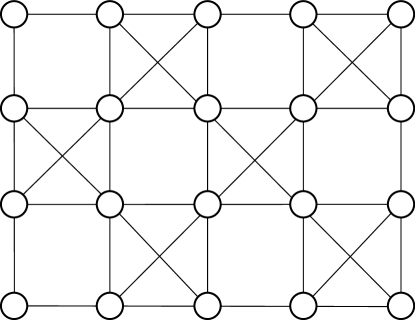
(a) IBM’s Q20 Tokyo

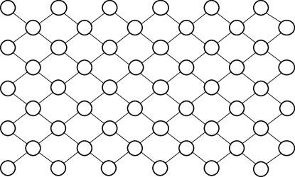
(b) Google’s Sycamore

Figure 1: The NISQ device architectures of IBM’s Q20 Tokyo and Google’s Sycamore are represented where each vertex symbolizes a qubit, and each edge signifies a coupler. Therefore, a controlled-NOT (CNOT) gate can directly execute between any two connected qubits.

The existing methods [22, 23] focus on optimizing the qubit placement layout for application-specific quantum circuits, aiming to optimize connectivity while considering physical constraints, such as frequency-collision effects, to improve fabrication yield rates. However, limited attention has been paid to the configuration of tunable-coupler superconducting quantum computers (SQCs). Lin et al. [24] proposed a method for finding an optimal layout using tunable couplers. However, this method did not consider the physical constraint imposed by frequency-collision effects. Our study bridges the gap by exploring coupling configurations for a specific input quantum circuit. It leverages the contextual connectivity correlation of the quantum circuit to minimize connections between noncorrelated qubits (i.e., without two-qubit gates) while enhancing fidelity and considering to the physical constraints of the SQC. We believe our approach can shed light on the benefits of initializing a layout for tunable coupler SQCs instead of dynamically tuning them during runtime, which can significantly affect qubit reliability.

To achieve this, we must address several key challenges related to the physical constraints of tunable-coupler QCs. Next, we must identify the contextual connectivity patterns within the input quantum circuit to discover the optimal connections. Afterward, we must determine the placement of physical qubits and their connections while ensuring that the final layout complies with the physical constraints of the SQC itself.

As a solution, we propose a Context-Aware COupler REconfiguration (CA-CORE) method, a compilation flow that considers the connectivity of the input circuit to find the optimal layout configuration. We design a circuit analysis that utilizes the correlation matrix between qubits to determine their connectivity weight. With this information, we construct a maximum weighted path graph (MWPG) that connects highly correlated qubits. Thereafter, we introduce an algorithm to generate a grid graph using the MWPG. Additionally, we propose a heuristic rule for eliminating connections that violate the SQC’s constraints on the grid graph. In summary, this study makes the following contributions:

• We propose CA-CORE, a compilation method for determining the optimal physical qubit-coupling map-layout configuration for a quantum circuit based on tunable coupler-based SQC.

• We introduce an algorithm for identifying a MWPG and apply it to construct a grid graph that incorporates both adjacent and diagonal edges while considering the contextual correlations of qubits.

• We evaluate the performance of our physical qubit-coupling map-layout configuration, which reduces the number of depth, gate, and SWAP required by up to 18.84%, 9.48%, and 42.47%, respectively. It also improves circuit fidelity by up to 40%, and compiles on a 33-qubit quantum circuit in less than 1$s$.

This paper is organized as follows. Section 2 discusses the background and motivation of our proposed method. The details of the context-aware coupling configuration are discussed in Section 3. In Section 4, we discuss the experimental setup and evaluation results. Section 5 focuses on the discussions and future works, whereas Section 6 presents related works. Finally, the paper is concluded in Section 7.

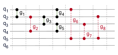
(a) Quantum Circuit

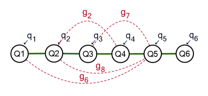
(b) Qubit Mapping on Line Graph

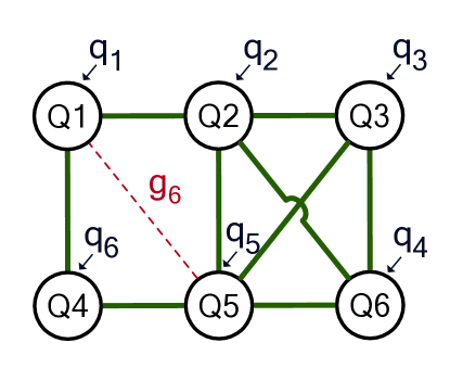
(c) Qubit Mapping on Grid Graph

Figure 2: Example of a quantum circuit with its corresponding interaction graph (IG). Each line and vertex represents a qubit. The green solid edge indicates that a CNOT gate can be directly executed between the two qubits, and the red dotted edge indicates that a CNOT gate cannot be directly executed between the two qubits.

2 Background and Motivation

Here, we provide the fundamentals for understanding our proposed method. We discuss the quantum computing basics of qubits, quantum operations, and quantum circuits. Thereafter, we discuss the coupler-based SQC hardware constraints, their physical properties, circuit fidelity, and the motivation behind our proposed method.

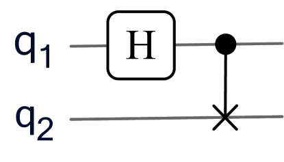
(a) Hadamard and CNOT gate

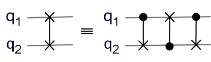
(b) SWAP gate with its equivalent decomposed gates

Figure 3: Basic quantum operations. Each horizontal line represents a qubit, and operations (gates) are applied to them, such as Hadamard (H), controlled-NOT (CNOT), SWAP (equivalent to three CNOT) gates.

2.1 Quantum Computing Basics

We begin with the basic concepts of quantum bits (qubits) and quantum operations, which were employed to create the quantum program and can be represented using quantum circuits.

Qubits and Quantum Operations: Quantum programs are composed of qubits and gates as the communication operations [25]. Figure 3 shows the quantum basic gates of single and multiple-qubit gates, such as Hadamard (H), Controlled-NOT (CNOT), and SWAP (equivalent to three CNOT) gates. A quantum circuit can be composed of as many qubits as needed denoted as $q$ and represented on horizontal lines in Figure 2(a). The choice of the gates can change the state of the quantum program, and there are two basis states denoted as $|0\rangle$ and $|1\rangle$. Additionally, SWAP gates can be as expensive as three equivalent CNOT gates. We assume that the SWAP gate is considered to have only one weight as the CNOT gate.

Quantum Circuit: An interaction graph (IG) is a graph that represents the interactions between the qubits in a quantum circuit [26, 23, 27]. The nodes in the graph represent the qubits $q$, and the edges in the graph represent the two-qubit gates of $q_{i}$ and $q_{j}$ as $g_{n}$, where $n$ is the number of interactions. To consider a logical circuit, we illustrate the quantum circuit of six qubits ($q_{1}$ to $q_{6}$) with the eight CNOT gates ($g_{1}$ to $g_{8}$) (see Figure 2(a)). For instance, gate $g_{1}$ represents the direct interaction between qubits $q_{1}$ and $q_{2}$, whereas gate $g_{2}$ represents the indirect interaction between qubits $q_{2}$ and $q_{4}$. IGs are employed to identify the qubits that can be placed far apart without affecting the circuit’s performance of the circuit. Consequently, it helps determine the number of qubit connections in the circuit from the logical to the physical level. This information define to the connectivity weight in this study.

2.2 Coupler-Based SQC Hardware Constraints

Quantum computing hardware can be developed using a variety of technologies, such as SQCs, ion traps, quantum dots, neutral atoms, etc. The SQC is currently one of the most promising technology. Shown in Figure 1 are the architecture of the IBM’s Q20 Tokyo, and Google’s Sycamore. During the NISQ era, all logical qubits must be directly implemented by physical qubits unaided by any QEC codes. This study considers two major limitations and constraints of NISQ hardware as context-aware to the model we employed to design coupler reconfiguration for tunable coupler-based SQCs.

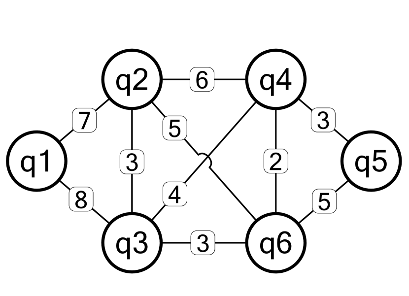
(a) Circuit Analysis

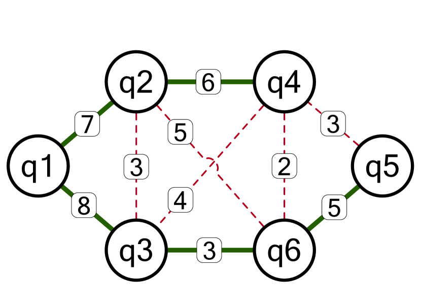
(b) Max Weighted Path Graph Generation

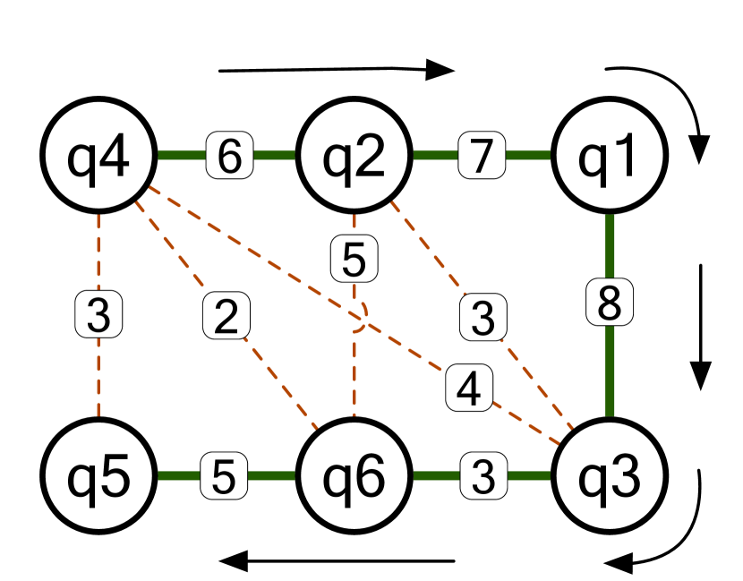
(c) Grid Graph
Generation

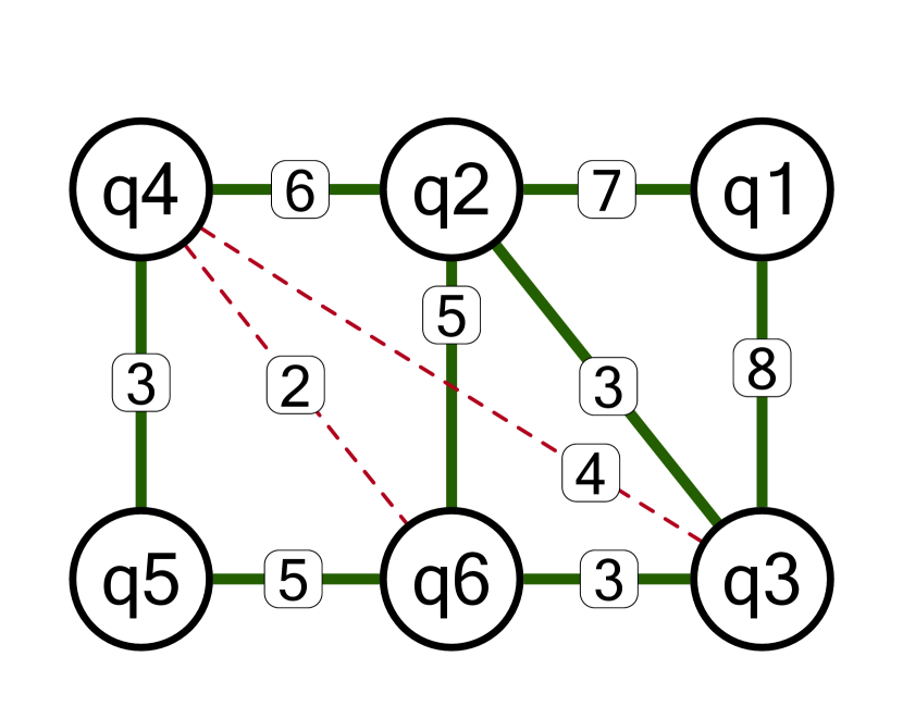
(d) Constraint
Configuration

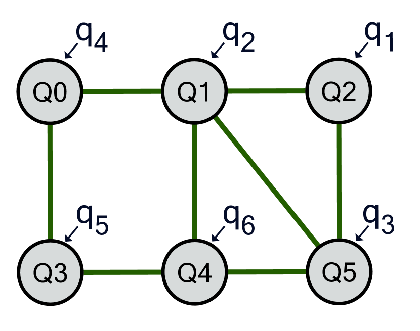
(e) Efficient Coupling Map

Figure 4: Overview of the coupling map generation process. (a) Analysis the contextual correlation between qubits; the coupling weight is assigned depending on the number of correlations between qubits. (b) Generation of the MWPG by connecting the highest weighted path (solid line). (c) and (d) Generation of the grid topology using MWPG and connecting the adjacent and diagonal edges, respectively. (e) Generated qubit physical layout coupling map.

SQC Physical Properties: Using two-qubit gates relies on physical connections, meaning superconducting qubits are confined to neighboring locations on a 2D plane. A popular coupling structure is the layout of qubits on IBM Q20 Tokyo’s superconducting quantum chip, as shown in Figure 1(a). In this coupler structure, there is a major constraint involving the diagonal coupler: continuous diagonal couplers introduce defects of dense frequency collisions on the device. Additionally, the vendor fabricates the qubits coupler in a regularized structure of $4\times 5$ lattices to reduce the fabrication complexity while ensuring the scalability and reliability of the coupling structure.

Quantum Circuit Fidelity: Notably, the previous problem is resolved to optimize qubit connection and maximize the overall performance against topologies by IBM and Google. Li et al. [28] reported the average error rates of a single-qubit gate and CNOT gate as $4.43\times 10^{-3}$ and $3.00\times 10^{-2}$, respectively. Due to on-chip placement constraints and routing constraints, couplers can only connect one qubit to its neighboring qubit.  [26, 29, 30]. Besides the physical properties, what we are concerned with the crosstalk error, which affects the quality of circuit fidelity. In this study, we investigate the contextual correlation between qubits, i.e., multi-qubit gates. We do not consider single-qubit gates because they do not incur additional qubit movement overhead during execution on any coupling structure.

2.3 Motivation

We employ a simple circuit of six qubits and eight gates to explain our motivation for considering qubit mapping, gate error, and different types of qubit architecture for determining the number of physical qubit coupler reconfigurations for tunable coupler-based SQCs.

Quantum circuit’s effect on qubit mapping: When executing a quantum circuit on a QC, the logical qubits need to be mapped to physical qubits on the target quantum architecture. For instance, the constraint of SQC architecture is 2D nearest neighbor qubits. Figure 2 demonstrates a simple example of the quantum circuit with a qubit mapping on different architectures of line and grid graphs.

Qubit mapping’s impact on the coupling map: Consider the example of Figure 2(b), where the original circuit is mapped onto the line graph with its physical constraints. Besides the indirect interaction of $g_{2}$, $g_{6}$, $g_{7}$ and $g_{8}$ denotes a red dotted line, other interactions can be mapped directly to the graph. In the same way, Figure 2(c) maps the same original circuit onto another graph of a grid graph with more physical connectivity. We can clearly observe that the red dotted lines that denote the indirect interactions reduce to only one which is $g_{6}$, compared with the features of the line graph qubit mapping.

In this instance, it is clear that a better initial mapping depends on the choice of architecture. Therefore, the bridging gap between the physical qubit graph and the qubit mapping problem can be addressed at the compilation level. This motivates us to propose a compilation method for determining the maximum physical qubit coupler reconfiguration for tunable coupler-based superconducting quantum computers (SQCs). This proposed method can resolve the indirect interactions of the remaining nonexecutable two-qubit gates of the qubit mapping problem, and compensate for the lack of connectivity on the physical qubit connectivity. Thus, this method offers more guaranteed advantages, such as lower compiled circuit depth, SWAP-gate-number reduction and fidelity improvement.

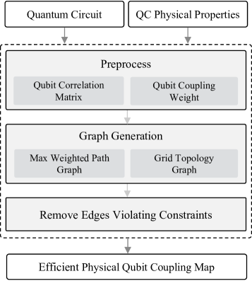
Figure 5: Overall architecture of the proposed method. We load the quantum circuit and QC physical properties as an input to design an efficient physical qubit coupling map.

3 Context-Aware Coupler Reconfiguration

This section covers CA-CORE, our method for context-aware coupling reconfiguration, explaining its architecture and implementation details.

3.1 Overall Architecture

To determine the optimal physical qubit coupling map-layout configuration for a quantum circuit, we must analyze the circuit to establish contextual correlations between logical qubits efficiently. This process involves assessing the two-qubit gates between logical qubits, with one-qubit gates being disregarded since they do not require any qubit movement during the execution process. For each two-qubit gate, we assign a weight to each qubit pair’s connection to create a correlation matrix. As illustrated in Figure 4(a), the circuit analysis provides the contextual correlation weights between qubits, with each qubit pair assigned a weight corresponding to the number of two-qubit gates interaction involved in the corresponding qubit pair.

Given that SQC processor adheres to a 2D grid shape [31, 32, 33, 34, 6], we need to reshape the graph from Figure 4(a) to conform to a grid-like structure. This adjustment should also account for the constraints imposed by the SQC’s physical construction, including the transmon qubits and couplers. Each qubit can connect to its neighbors in all directions (grid); however, diagonal edges are prohibited when neighboring connections already include diagonal edges (except diagonal neighbor) [23, 35].

To achieve this, we tailor the circuit graph to minimize qubit movement and distance while maximizing the weight using an MWPG. Figure 4(b) shows an MWPG subject to constraints where each node can only have two edges and loops are disallowed. The black (straight) lines represent the maximum weighted path, while the red (dotted) lines indicate edges eliminated for violating the path graph constraints.

We employ this method to construct a path graph while maximizing the edges with the highest weights. Subsequently, we transform the MWPG into a grid graph while considering the constraints discussed in Section 2.2. As shown in Figure 4(c), this grid graph retains the maximum weighted path and facilitates the connection of adjacent and diagonal edges between nodes. Figure 4(d) shows an example where the edges between $q_{2}$ to $q_{6}$ and $q_{2}$ to $q_{3}$ can be connected, as these connections adhere to the allowed constraints. However, the edge between $q_{4}$ and $q_{6}$ cannot be connected, as the connection violates the constraints. The decision to connect $q_{2}$ and $q_{3}$ over $q_{4}$ and $q_{6}$ is based on the edge weights, with the former having a weight of 3 and the latter having a weight of 2.

After completing these processes, the grid graph constructed in Figure 4(d) can be employed to establish a physical qubit-coupling map, as shown in Figure 4(e). All allowed edges are utilized to form the couplers for the qubits. The result is an efficient qubit coupling map for the input circuit. Thus far, we have presented an overview of the entire process and the objectives of our proposed method using a small quantum circuit with only six qubits. To delve into the details of each implementation step, particularly for large quantum circuits, we can refer to the overall proposed architecture described in Figure 5.

The algorithm begins the prepossess by analyzing the input quantum circuit to extract the coupling map (edges) and its correlation weight matrix. The coupling map is established by detecting connections between qubits via two-qubit gates. Whenever two qubits are connected in this manner, they are considered a pair or a coupling. Meanwhile, for the correlation weight matrix, we assign a weight of 1 to each two-qubit gate present in the quantum circuit.

Using contextual results obtained from the analysis of the coupling map and the correlation matrix, we can subsequently proceed to configure an efficient qubit coupling map layout.

3.2 Max Weighted Path Graph Generation

Input:

$qc\_graph$: original quantum circuit graph,

$c\_weight$: qubit coupling weight correlation

Output:

$path\_graph$ : max weighted path graph

Function  generate_max_weighted_path_graph

       $path\_graph$ = initial empty graph;

      $sorted\_edge$ = get sort weighted edges in $c\_weight$;

      for $edge$ in $sorted\_edge$ do

             // extract info from edge

             $n1$, $n2$, $weight$ = $edge$;

            // max connection validation

             if $n1.neighbors>=2$ or $n2.neighbors>=2$ then

                   // only allow max 2 edges

                   continue;

             end if

            

            // loop connection validation

             $tmp\_path\_graph$ = $path\_graph$;

             add $edge(n1,n2)$ to $tmp\_path\_graph$;

             if $tmp\_path\_graph.has\_loop\_subgraph$ then

                   // loop is not allowed

                   continue;

             end if

            

            add $edge(n1,n2,weight)$ to $path\_graph$;

            

       end for

      return $path\_graph$;

end

ALGORITHM 1 Max Weighted Path Graph Generation

As we discussed in the previous section, the topology of the quantum circuit resembles a grid, featuring both adjacent and diagonal edges. Consequently, the configured qubit coupling map topology should follow to this grid-like format. To achieve an efficient grid-like layout, we initiate the process by generating a MWPG using the logical coupling map and correlation data obtained from the analyzed circuit. The MWPG is employed because it can be efficiently transformed into the desired grid-like structure with a specified number of rows and columns. Moreover, it can accommodate qubit layouts characterized by high correlations between individual qubits.

Algorithm 1 outlines the procedure for generating an MWPG based on the logical qubit-coupling weight correlations defined as c_weight. There are two conditions that an MWPG must adhere to, as follows: 1) A single logical qubit n cannot have more than 2 edges or neighbors connections with other qubits. 2) Loops are not permitted; to effect this, we make a temporary path graph (tmp_path_graph) with all the edges and nodes from the original path_graph. Thereafter, we add the edges with two qubits (n1 and n2) to tmp_path_graph. A subsequent verification process is then carried out to detect the presence of any loops within this temporary graph. In this process, logical couplings with the highest weights are constructed first, followed by those with lower weights. If a coupling fails to meet the mentioned conditions, no coupling connection will form.

An issue may emerge based on the contextual correlation of the quantum circuit when certain qubits lack of connection with others. In such instances, our MWPG might contain multiple isolated subgraphs. To resolve this, we connect these subgraphs by identifying logical qubits with a single connection, maintaining the prior constraints.

3.3 Grid Topology Generation

Input:

$nrow$: number of rows for grid topology,

$ncol$: number of columns for grid topology,

$c\_weight$: qubit coupling weight correlation,

$path\_graph$: max weighted path graph

Output:

$grid\_graph$ : grid graph with adjacency and diagonal edges

Function  generate_grid_topology_graph

       // assign node to $pos\_matrix$ to determine the position of the node in the grid graph

       $pos\_matrix$ = put $path\_graph$’s node by shape $row$ x $col$;

      

      $grid\_graph$ = get all nodes and edges from $path\_graph$;

      

      // connect adjacent edges

       for $row\leftarrow 0$ to $nrow-1$ do

             for $col\leftarrow 0$ to $ncol$ do

                   $n1$ = $pos\_matrix[row][col]$;

                   $n2$ = $pos\_matrix[row+1][col]$;

                  

                  if $not$ $c\_weight.has\_edge(n1,n2)$ then

                         continue;

                   end if

                  $grid\_graph.add(n1,n2)$

             end for

            

       end for

      // connect diagonal edges

       for $row\leftarrow 0$ to $nrow-1$ do

             for $col\leftarrow 0$ to $ncol$ do

                   $n1$ = $pos\_matrix[row][col]$;

                   // left lower diagonal edge

                   if $col>0$ then

                         $n2\_left$ = $pos\_matrix[row+1][col-1]$;

                         if $not$ $c\_weight.has\_edge(n1,n2\_left)$ then

                               continue;

                         end if

                        $grid\_graph.add(n1,n2\_left$

                   end if

                  // right lower diagonal edge

                   if $col+1<ncol$ then

                         $n2\_right$ = $pos\_matrix[row+1][col+1]$;

                         if $not$ $c\_weight.has\_edge(n1,n2\_right)$ then

                               continue;

                         end if

                        

                        $grid\_graph.add(n1,n2\_right)$

                   end if

                  

             end for

            

       end for

      

      return $grid\_graph$;

end

ALGORITHM 2 Grid Topology Generation

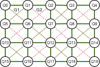
Figure 6: Physical qubit grid topology graph configuration with all possible edges. Diagonal edges are separated into G1: solid (black) line and G2: dotted (red) line. Each group represents possible diagonal edge configurations that conform to the maximum diagonal edges allowed while considering to the physical constraints of SQC.

In Figures 4(b) and 4(c), the grid graph is created by arranging nodes adjacent to each other in rows and columns. To initialize the grid graph to construct our proposed MWPG, we select either the first or last node of the path and position them in a row and column format. Thereafter, we connect it to all of the path nodes through edges.

To implement this in a programming model, as shown in Algorithm 2, we utilize a position matrix (pos_matrix) to determine the position of each logical qubit by placing its node position from MWPG in the matrix. Afterward, we connect the logical qubits in adjacent positions only if their qubit coupling-weight (c_weight) are correlated. The adjacent edge can be formed using pos_matrix by iterating through each row and column (col). In each col, the position of n1 in the pos_matrix is located at index pos_matrix[row][col]. Meanwhile, its adjacent edge, n2, is positioned at index pos_matrix [row+1][col]. Essentially, the adjacent edge of n1 is situated at its bottom in the grid graph. As depicted in Figure 4(c), n1 is represented by the q4 in the first row and first column, whereas its adjacent edge, n2, is represented by q5 in the second row and first column.

For the diagonal edges, we initiate the connection process starting from the first row and first column. Each logical qubit in the first row checks the availability of its left and right diagonal edges through the pos_matrix, constructing an edge only when the c_weight values are correlated. The left diagonal edge of n1, referred to as n2_left, can be located at the bottom-left of its position within the grid_graph, with index pos_matrix[row+1][col-1]. It exists only when the condition, $col>0$ is satisfied, meaning that n2_left is absent if n1 is positioned at the extreme left of the grid_graph. As for the right diagonal edge, denoted as n2_right, it can be found at index pos_matrix[row+1][col+1]. It exists only when the condition $col+1<ncol$ is met, signifying that there is no n2_right if n1 is at the far right of the grid_graph. For an example, please refer to Figure 4(d), where q2, q5, and q3 represent n1, n2_left, n2_right, respectively.

Upon connecting all correlated adjacency and diagonal edges, we obtain a grid graph that maximizes connections for logical qubits, ensuring that all possible edges are established. This minimizes travel distances between correlated qubits, while minimizing unnecessary coupling connections. Notably, throughout this process, we did not considered the physical constraints associated with diagonal edge connections. This concern will be addressed more precisely in the following section.

3.4 Eliminating Constraints on Diagonal Edges

To address the constraints imposed by the physical qubits of the SQC, as discussed in Section 2.2, we must consider which possible configuration of diagonal edges carries greater weight. To achieve this, we partition the diagonal edges into two groups, each accumulating the combined weight of diagonal edges that can coexist within the grid graph. As shown in Figure 6, a grid graph with all possible edges connected is depicted. The diagonal edges are separated into two groups: Group 1 (G1) and Group 2 (G2). G1 contains all the diagonal edges with solid (black) lines, whereas G2 comprises all the diagonal edges with dotted (red) lines. In CA-CORE, such a reconfigured topology graph is only generated when the quantum circuit contains fully connected qubits, meaning that each qubit has correlations with all the other qubits in the quantum circuit.

We begin accumulating the weight of the edges for G1, starting from the first row and first column. Each group within each row and column consists of two pairs of diagonal edges between physical qubits, with the weight of each edge being added to the group. Subsequently, moving to the first row and the second column of physical qubits, another two pairs of diagonal edges to the right can be accumulated. However, this time, the accumulated weight belongs to G2. This process continues until no more neighboring qubits are to the right of a given position. Subsequently, the group orientation needs to be flipped in the second row, as demonstrated in Figure 6.

Finally, we eliminate the diagonal edges from the group that has accumulated the lowest weight. The resulting grid graph serves as the basis for constructing the layout of the physical qubit topology. This topology layout maximizes the correlation weight of the logical qubits while adhering to the constraints of the SQC itself.

Num of Qubit	CA-CORE to Almaden (20)			CA-CORE to Cairo (27)			CA-CORE to Prague (33)			CA-CORE to Sycamore (53)
	Depth	Gate	SWAP	Depth	Gate	SWAP	Depth	Gate	SWAP	Depth	Gate	SWAP
10	10.54%	4.23%	35.09%	10.02%	8.04%	51.69%	10.68%	8.09%	51.87%	6.60%	5.01%	39.21%
11	10.66%	5.55%	41.35%	13.03%	9.02%	54.31%	13.28%	9.22%	54.92%	7.92%	5.89%	42.89%
12	11.45%	5.57%	39.04%	13.39%	8.71%	50.88%	12.97%	8.43%	49.98%	8.58%	5.56%	39.00%
13	12.51%	5.50%	35.59%	12.68%	8.26%	46.10%	13.76%	8.75%	47.67%	9.01%	6.36%	39.20%
14	10.42%	4.83%	32.32%	11.28%	7.53%	43.42%	12.53%	7.89%	44.66%	7.54%	5.53%	35.52%
15	11.59%	4.53%	30.17%	13.51%	7.25%	41.59%	14.75%	7.86%	43.73%	10.18%	6.02%	36.86%
16	10.76%	4.86%	30.53%	15.07%	7.85%	42.29%	14.22%	7.41%	40.79%	8.23%	4.80%	30.27%
17	13.11%	5.00%	29.77%	17.04%	7.94%	41.00%	16.74%	7.59%	39.82%	10.46%	5.84%	33.33%
18	11.59%	5.52%	31.74%	17.42%	8.65%	43.00%	17.72%	9.00%	44.06%	9.13%	5.74%	32.65%
19	13.34%	5.45%	29.86%	19.92%	9.22%	42.87%	18.60%	9.27%	43.00%	7.87%	5.08%	28.34%
20	12.18%	4.91%	26.07%	19.01%	9.44%	41.59%	18.33%	9.90%	42.86%	6.67%	4.88%	25.93%
21	-	-	-	19.36%	9.24%	39.99%	18.82%	9.14%	39.70%	6.20%	3.98%	21.34%
22	-	-	-	17.94%	9.17%	39.17%	19.64%	9.60%	40.36%	5.25%	3.70%	19.67%
23	-	-	-	19.50%	9.92%	39.99%	18.95%	10.32%	41.04%	7.63%	4.54%	22.33%
24	-	-	-	20.37%	9.67%	38.77%	18.46%	9.25%	37.60%	8.48%	3.92%	19.45%
25	-	-	-	18.58%	8.45%	34.05%	20.17%	8.87%	35.26%	7.05%	3.54%	17.05%
26	-	-	-	21.10%	9.62%	38.81%	20.81%	9.70%	39.03%	7.44%	4.44%	21.68%
27	-	-	-	20.34%	9.01%	34.87%	19.27%	9.41%	35.98%	3.40%	2.59%	12.58%
28	-	-	-	-	-	-	21.50%	10.68%	40.02%	6.75%	3.93%	18.59%
29	-	-	-	-	-	-	22.22%	10.67%	39.56%	6.41%	3.69%	17.36%
30	-	-	-	-	-	-	25.23%	11.57%	40.82%	8.62%	4.46%	19.74%
31	-	-	-	-	-	-	24.50%	11.11%	39.62%	7.78%	3.83%	17.30%
32	-	-	-	-	-	-	23.40%	11.12%	38.70%	5.06%	3.48%	15.39%
33	-	-	-	-	-	-	27.07%	12.75%	42.77%	7.58%	3.60%	16.04%
Average:	11.65%	5.09%	32.87%	16.64%	8.72%	42.47%	18.48%	9.48%	42.24%	7.49%	4.60%	25.91%

Table 1: Comparison of the number of depth, gate, and SWAP-gate-number reduction performances between our compiled CA-CORE and various existing topologies, including IBM’s ibmq_almaden 20-qubit, ibmq_cairo 27-qubit, and ibmq_prague 33-qubit systems, as well as Google’s Sycamore 53-qubit system. Ten randomly generated quantum circuits with approximately 2000-gate and 200-depth on average were evaluated for each qubit count, and their average results were computed individually.

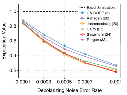
(a) ‘bigadder_n18’ Circuit

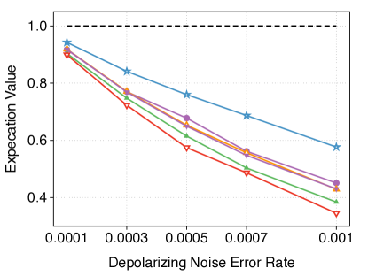
(b) ‘qec9xz_n17’ Circuit

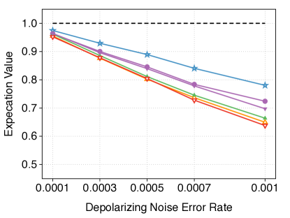
(c) ‘bv_n14’ Circuit

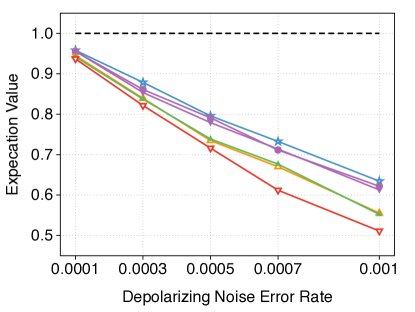
(d) ‘bv_n19’ Circuit

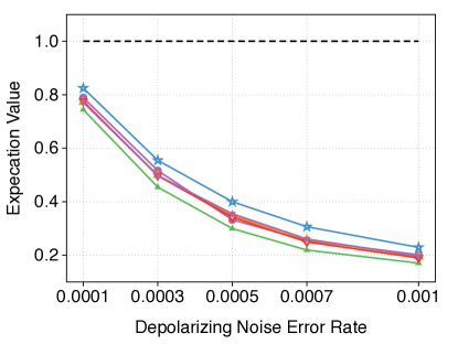
(e) ‘multiplier_n15’ Circuit

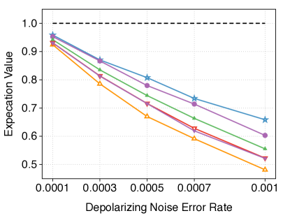
(f) ‘multiply_n13’ Circuit

Figure 7: Experiments involve applying a depolarizing noise model to execute the NISQ benchmark quantum circuit from [36] on CA-CORE. These results are then compared with outcomes obtained from various topologies. The collected results are compared with the Exact Simulation’s expectation value, which remains unaffected by noise. Consequently, the fidelity of exact simulation is 1. A result from various topologies closer to 1 indicates a higher fidelity.

4 Evaluation

In this section, we present the evaluation of CA-CORE compared with various existing topologies, in terms of depth, gate, and SWAP-gate-number reduction, and fidelity improvement.

4.1 Experiment Setup

Benchmarks. We generate random quantum circuits using Qiskit [37], ranging from 10-qubit to 33-qubit configurations. These circuits span up to approximately 200 depths and 3000 gates. This allows us to assess the performance regarding reductions in depth, gates, and SWAP operations. Furthermore, we utilize the low-level QASM benchmarks sourced from [36], which are well-suited for NISQ evaluation and simulation. These benchmarks aid in assessing noise-tolerant performance, given their considerable depth. Moreover, their expectation values can be simulated classically, enabling the extraction of precise results.

Hardware Topology. We compare the compiled CA-CORE with the the existing diversity of fixed-coupling device topologies, such as ‘ibmq_almaden,’ ‘ibmq_cairo,’ and ‘ibmq_prague’ available on Qiskit [37]. Furthermore, we generated a topology inspired by Google’s Sycamore architecture [6].

Experiment Platform. All experiments presented in this paper were conducted on a server with an AMD Ryzen 5955WX (32 logical cores) CPU, 512GB of memory, and 3 Nvidia RTX 4090 GPUs.

Algorithm Configuration. Our proposed method was setup to compile circuits to a topology where the number of physical qubits matches the number of logical qubits in the quantum circuit. Couplers are configured only when a correlation (a two-qubit gate) between logical qubits exists. The grid size is adjusted to accommodate based on the required number of qubits.

4.2 Depth, Gate, and SWAP-gate-number Reduction

To assess the performance of our CA-CORE in terms of depth, gate, and SWAP-gate-number reduction, we conducted experiments using 10 different randomly generated quantum circuits for each qubit count, as mentioned in Section 4.1 of our setup benchmarks. This approach aims to evaluate the diversity of the contextual qubit correlation, as opposed to using practical circuits that typically exhibit specific patterns in their qubit correlations.

To determine the number of gates, depth, and SWAP operations for all topologies mentioned in Section 4.1, including CA-CORE, we utilize Qiskit’s transpiler. We configure a custom coupling map setup and set the optimization_level to $0$. In this configuration, Qiskit applies minimal optimization, primarily focusing on basic qubit mapping, where logical qubit 0 is mapped to physical qubit 0, and so forth. Subsequently, SWAP gates are inserted for logical qubits that lack connectivity.

Table 1 presents theresults of the performancecomparison between CA-CORE and all benchmark topologies, in terms of depth, gate, and SWAP-gate-number reductions. On average, CA-CORE demonstrates improvements of $13.56\%$, $6.97\%$, and $35.87\%$ for of depth, gate, and SWAP operations, respectively. Specifically, for the 30-qubit circuit, CA-CORE employs the coupling-map configuration depicted in Figure 8(b). In this setup, CA-CORE utilizes diagonal couplings, resulting in reductions of $8.62\%$, $4.46\%$, and $17.30\%$ for depth, gate, and SWAP counts, respectively, in contrast to the result of the Sycamore coupling map, as illustrated in Figure 1(b). The primary distinction between the two configurations lies in the additional diagonal couplings among qubits, demonstrating that integrating these essential coupler connections significantly enhances the performance.

Regarding the gate and depth-reduction count, in our analysis, we treat each SWAP gate as a single gate, and we do not consider it as a three-CNOT gate decomposition. This means that a SWAP gate is counted as one gate when summing all the gates in the circuit. The depth count reflects the level of efficient parallel execution and reduction in SWAP path overhead within the quantum system, considering its topological setup.

4.3 Fidelity Improvement

To assess noise impact on CA-CORE, we use a depolarizing noise model with an error rate of $\epsilon$. This model assumes uniform error rates for all gates: $\epsilon$ for one-qubit channels and $\epsilon\times 5$ for two-qubit channels like the CNOT gate, making the latter five times more error-prone.

Figure 7 depicts the performance of our CA-CORE architecture compared with those of various topologies mentioned in Section 4.1. For IBM topologies, we use the original configuration, however, for Google’s Sycamore, which has 53 qubits, efficient simulation using a noise model is not feasible. Therefore, we employ a half-Sycamore topology setup with six rows and four columns, with all couplers enabled.

CA-CORE outperforms existing topologies in all evaluations. Particularly noteworthy is the 40.13% improvement in fidelity at an error rate ($\epsilon$) of 0.001 compared with the result achieved by Sycamore, as shown in Figure 7(b). On average for all error rate, CA-CORE exhibits fidelity improvements of 15.76%, 16.39%, 7.52%, 5.69%, 13.91%, and 9.77%, as shown in Figure 7(a),  7(b),  7(c),  7(d),  7(e), and 7(f), respectively.

Notably, in the result shown in Figure 7(d) for the ‘bv_n19’ circuit, the improvement is not significant at lower error rates. The ‘bv_n19’ circuit represents the Bernstein-Vazirani algorithm [38]. This algorithm requires a brief quantum circuit with two H gates for all qubits, one NOT (X) gate, and $n-1$ CNOT gates, where $n$ is the qubit count. Each CNOT gate connects all qubits with the last one. This structure ensures that at lower error rates, errors across different setups have minimal impact on result fidelity. Further, notably, Sycamore (24) performs worse compared to all the other topologies. This is primarily because the experiment was performed by employing basic qubit-mapping method. For the compiled circuit on various topologies, the circuit depths are as follows: 40 for CA-CORE, 43 for ibmq_almaden, 49 for ibmq_johannesburg, 48 for ibmq_cairo, 53 for Google’s Sycamore (24), and 45 for ibmq_prague. With differences in circuit depth, the impact of relatively high error rates also increases, contributing to the inferior performance of Google Sycamore’s topology. This contributes to the marginal improvement seen in CA-CORE compared to existing topologies across low-to-higher error-rate configurations.

4.4 Scalable Time Complexity

In the reprocessing step, an input graph of $n$ qubits is prioritized, where each qubit can connect to any other. This phase identifies all qubit correlations and their coupling weights with a time complexity of $O(n^{2})$. Then, Algorithm 1 constructs a new graph to maximize the weighted path using the obtained qubit connections from the preprocessing phase. In the new path graph, each qubit aligns to have a maximum of two adjacent connections, excluding loop connections. Next, the path graph is converted into a structured grid graph using Algorithm 2, specifying the desired columns and rows, with a time complexity of $O(n)$ for this transformation. The final step involves connecting the grid’s qubits based on the discovered connections during preprocessing, with a time complexity of $O(E)$, where $E$ represents the original graph’s connections. Furthermore, constraint removal adds another $O(E)$ in the worst case to calculate the weight of the violated constraint on the connectivity. Therefore, the total time complexity of the algorithm is $O(n^{2}+n+2E)$. With this time complexity, our algorithm can efficiently reconfigure the topology for the input quantum circuit. It takes less than 1$s$ to configure a topology for the 33-qubit quantum circuit used in benchmark Table 1.

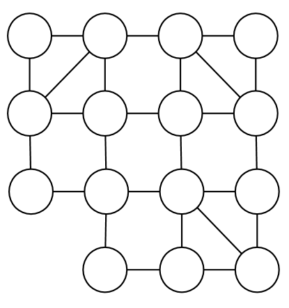
(a) ’multiplier_n15’

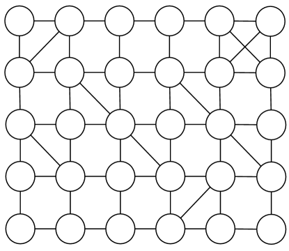
(b) ’Random Circuit 30-Qubit’

Figure 8: Our topology reconfigured for specific quantum circuits. (a) Reconfigured topology for ‘multipler_n15’ circuit benchmark in Figure 7(e). (b) Reconfigured topology for the randomly generated 30-qubit circuit benchmark in Table 1.

5 Discussion and Future Work

This study explores methods to adjust qubit connections within a tunable coupler SQC implemented in a grid topology setup. The adoption of a grid-like structure is influenced by previous studies [22, 23] demonstrating high yield with optimal connectivity. Specifically, we formalize the configured topology in three steps, each of which considers the correlations between qubits. To the best of our knowledge, this is the first study to utilize a quantum circuit for efficient coupling configuration while addressing the frequency-collision constraint of the SQC.

The manuscript refrains from directly comparing the proposed qubit mapping methodology with existing approaches due to a fundamental divergence in their focal points. Existing qubit mapping strategies predominantly concentrate on fixed topology target quantum hardware, aiming to optimize within the constraints of predetermined qubit layouts. In contrast, the manuscript’s emphasis lies in configuring optimal qubit coupling maps, specifically targeting tunable coupler-based quantum hardware. As a result, the comparison isn’t directly pursued as the existing qubit mapping techniques are tailored to a different paradigm, focusing on fixed hardware configurations, whereas the manuscript’s methodologies are designed for systems with tunable coupler features, warranting a distinct evaluation approach

While our proposed method efficiently identifies an optimal coupling map, reducing the need for additional SWAP operations and enhancing the fidelity of the input quantum circuit, further improvements and experiments are required.

Integrating Qubit Mapping Optimization: Many qubit mapping problems consider fixed connectivity on the target hardware. While our evaluation employs a basic qubit mapping approach, we anticipate that a well-designed qubit mapping solution, which considers the reconfigurable topology of the target hardware, can yield a significantly optimized topology.

Design Space and Frequency Allocation: Our study adheres to the design space, constraints, and frequency allocation configuration outlined in references [22, 23]. As quantum hardware fabrication techniques advance, additional studies should be undertaken to accommodate diverse quantum hardware configurations.

Real QC Evaluation: Our study outlines innovative methods for optimizing qubit coupling maps in quantum circuits, emphasizing efficiency and error reduction. While simulations form a strong foundation, exploring disparities between simulated and real-world outcomes would enrich the manuscript. Analyzing trade-offs between runtime coupler tuning and swap gate introduction offers insights for developers and users. Assessing how optimized layouts impact specific quantum algorithms clarifies practical implications. Looking ahead, our pioneering work in configuring optimal physical qubit coupling map layouts requires experimental validation on real quantum hardware. Collaborations with quantum computing experts or accessing tunable-coupler devices provide invaluable insights for real quantum computing. Investigating scalability, refining hardware-based constraints, and exploring error mitigation strategies are essential for future research, bridging theory with practical applications.

6 Related Work

Various studies have been conducted on tunable coupler-based SQCs and qubit coupling map layouts [39, 23, 40]. Tunable two-qubit couplers have shown potential for application in mitigating errors within multi-qubit gate in SQC processors [40]. Additionally, architectures have been proposed for both the modular implementation of tunable couplers [41] and the utilization of floating tunable couplers in designs of large-scale quantum processors [42].

These studies primarily emphasize the design of tunable couplers to enhance the scalability of SQC processors. Gushu et al. [23] emphasized a logical qubit coupling topology and construct the hardware architecture using three subroutines: layout design, bus selection, and frequency allocation. This was achieved while considering physical constraints based on the profiling information from the coupling degree list and the coupling strength matrix. Their primary objective was to enhance the yield rate by maximizing qubit connectivity. However, they did not address the noise implications of their architecture. Tan et al. [43] presented QLSA-reconfigurable-atomic-arrays (RAA), a layout synthesizer RAA during the QC compilation phase. While their method achieves gate reduction and heightened fidelity for reconfigurable architectures through hardware-adaptive constraints, it is specifically designed for atomic arrays. Conversely, our proposed approach addresses the constraints inherent in SQCs.

Lin et al. [24] proposed a method similar to ours which utilizes layout synthesis to establish qubit edge connections. However, the edges they determined contradict the fabrication constraints due to the frequency collision outlined in [22, 23]. Conversely, our proposed method considers the edge connection that adheres to the frequency collision constraint, maximizing the SQC’s connectivity. Given these contradictions and disparities in architectural design for edge selection, we cannot conduct a comparative study between their method and our method.

7 Conclusion

Quantum algorithms demand extensive resources that often surpass the available quantum hardware capacity. However, the design of application-specific architectures for quantum algorithms can help reduce the required quantum resources while enhancing result fidelity. This study delves into the benefits of initializing an optimal layout for a target quantum algorithm on a tunable coupler-based SQC to eliminate unnecessary connections between uncorrelated qubits. This involves an analysis of the input circuit to determine the contextual correlation matrix between qubits and their connectivity weights. Subsequently, we propose an algorithm to configure a grid-like topology, considering qubit correlations and the physical constraints of the SQC. Experimental results demonstrate that the context-aware reconfigured topology can reduce circuit depth by minimizing additional SWAP operations in a randomly generated quantum circuit with a complex pattern while improving output fidelity in practical NISQ benchmark circuits.

References

- [1] Lov K. Grover. “A fast quantum mechanical algorithm for database search”. In Proceedings of the Twenty-Eighth Annual ACM Symposium on Theory of Computing. Page 212–219. STOC ’96New York, NY, USA (1996). Association for Computing Machinery.
- [2] Peter W Shor. “Algorithms for quantum computation: discrete logarithms and factoring”. In Proceedings 35th annual symposium on foundations of computer science. Pages 124–134. Ieee (1994).
- [3] Gary J Mooney, Gregory AL White, Charles D Hill, and Lloyd CL Hollenberg. “Whole-device entanglement in a 65-qubit superconducting quantum computer”. Advanced Quantum Technologies 4, 2100061 (2021).
- [4] Prakash Murali, Dripto M Debroy, Kenneth R Brown, and Margaret Martonosi. “Architecting noisy intermediate-scale trapped ion quantum computers”. In 2020 ACM/IEEE 47th Annual International Symposium on Computer Architecture (ISCA). Pages 529–542. IEEE (2020).
- [5] Charles Q Choi. “Ibm’s quantum leap: The company will take quantum tech past the 1,000-qubit mark in 2023”. IEEE Spectrum 60, 46–47 (2023).
- [6] Frank Arute, Kunal Arya, Ryan Babbush, Dave Bacon, Joseph C Bardin, Rami Barends, Rupak Biswas, Sergio Boixo, Fernando GSL Brandao, David A Buell, et al. “Quantum supremacy using a programmable superconducting processor”. Nature 574, 505–510 (2019).
- [7] Erik J Gustafson, Andy CY Li, Abid Khan, Abid Kahn, Joonho Kim, Doga Murat Kurkcuoglu, M Sohaib Alam, Peter P Orth, Armin Rahmani, and Thomas Iadecola. “Preparing quantum many-body scar states on quantum computers”. Technical report. Fermi National Accelerator Lab.(FNAL), Batavia, IL (United States) (2023).
- [8] Joanna Śliwa and Konrad Wrona. “Quantum computing application opportunities in military scenarios”. In 2023 International Conference on Military Communications and Information Systems (ICMCIS). Pages 1–10. IEEE (2023).
- [9] Salonik Resch and Ulya R. Karpuzcu. “Benchmarking quantum computers and the impact of quantum noise”. ACM Comput. Surv.54 (2021).
- [10] Nikita Acharya, Miroslav Urbanek, Wibe A De Jong, and Samah Mohamed Saeed. “Test points for online monitoring of quantum circuits”. ACM Journal on Emerging Technologies in Computing Systems (JETC) 18, 1–19 (2021).
- [11] Abdullah Ash Saki, Mahabubul Alam, Koustubh Phalak, Aakarshitha Suresh, Rasit Onur Topaloglu, and Swaroop Ghosh. “A survey and tutorial on security and resilience of quantum computing”. In 2021 IEEE European Test Symposium (ETS). Pages 1–10. IEEE (2021).
- [12] Yang Qian, Zhijin Guan, Shenggen Zheng, and Shiguang Feng. “A method based on timing weight priority and distance optimization for quantum circuit transformation”. Entropy 25, 465 (2023).
- [13] Ellis Wilson, Sudhakar Singh, and Frank Mueller. “Just-in-time quantum circuit transpilation reduces noise”. In 2020 IEEE international conference on quantum computing and engineering (QCE). Pages 345–355. IEEE (2020).
- [14] Jinzhao Sun, Xiao Yuan, Takahiro Tsunoda, Vlatko Vedral, Simon C Benjamin, and Suguru Endo. “Mitigating realistic noise in practical noisy intermediate-scale quantum devices”. Physical Review Applied 15, 034026 (2021).
- [15] Yongshan Ding, Pranav Gokhale, Sophia Fuhui Lin, Richard Rines, Thomas Propson, and Frederic T Chong. “Systematic crosstalk mitigation for superconducting qubits via frequency-aware compilation”. In 2020 53rd Annual IEEE/ACM International Symposium on Microarchitecture (MICRO). Pages 201–214. IEEE (2020).
- [16] Prakash Murali, David C McKay, Margaret Martonosi, and Ali Javadi-Abhari. “Software mitigation of crosstalk on noisy intermediate-scale quantum computers”. In Proceedings of the Twenty-Fifth International Conference on Architectural Support for Programming Languages and Operating Systems. Pages 1001–1016. (2020).
- [17] Soheil Khadirsharbiyani, Movahhed Sadeghi, Mostafa Eghbali Zarch, Jagadish Kotra, and Mahmut Taylan Kandemir. “Trim: crosstalk-aware qubit mapping for multiprogrammed quantum systems”. In 2023 IEEE International Conference on Quantum Software (QSW). Pages 138–148. IEEE (2023).
- [18] Lei Xie, Jidong Zhai, and Weimin Zheng. “Mitigating crosstalk in quantum computers through commutativity-based instruction reordering”. In 2021 58th ACM/IEEE Design Automation Conference (DAC). Pages 445–450. IEEE (2021).
- [19] Dripto M Debroy, Muyuan Li, Shilin Huang, and Kenneth R Brown. “Logical performance of 9 qubit compass codes in ion traps with crosstalk errors”. Quantum Science and Technology 5, 034002 (2020).
- [20] Jonathan Wei Zhong Lau, Kian Hwee Lim, Harshank Shrotriya, and Leong Chuan Kwek. “Nisq computing: where are we and where do we go?”. AAPPS Bulletin 32, 27 (2022).
- [21] Hui Wang, Yan-Jun Zhao, Hui-Chen Sun, Xun-Wei Xu, Yong Li, Yarui Zheng, Qiang Liu, and Rengang Li. “Controlling the qubit-qubit coupling in the superconducting circuit with double-resonator couplers”. Physical Review A109 (2024).
- [22] Tian Yang, Weilong Wang, Lixin Wang, Bo Zhao, Chen Liang, and Zheng Shan. “A superconducting quantum processor architecture design method for improving performance and reducing frequency collisions”. Results in Physics 53, 106944 (2023).
- [23] Gushu Li, Yufei Ding, and Yuan Xie. “Towards efficient superconducting quantum processor architecture design”. In Proceedings of the Twenty-Fifth International Conference on Architectural Support for Programming Languages and Operating Systems. Pages 1031–1045. (2020).
- [24] Wan-Hsuan Lin, Bochen Tan, Murphy Yuezhen Niu, Jason Kimko, and Jason Cong. “Domain-specific quantum architecture optimization”. IEEE Journal on Emerging and Selected Topics in Circuits and Systems 12, 624–637 (2022).
- [25] Ivan B Djordjevic. “Quantum communication, quantum networks, and quantum sensing”. Academic Press. (2022).
- [26] Marcos Yukio Siraichi, Vinícius Fernandes dos Santos, Caroline Collange, and Fernando Magno Quintão Pereira. “Qubit allocation”. In Proceedings of the 2018 International Symposium on Code Generation and Optimization. Pages 113–125. (2018).
- [27] Medina Bandic, Carmen G Almudever, and Sebastian Feld. “Interaction graph-based characterization of quantum benchmarks for improving quantum circuit mapping techniques”. Quantum Machine Intelligence 5, 40 (2023).
- [28] Gushu Li, Yufei Ding, and Yuan Xie. “Tackling the qubit mapping problem for nisq-era quantum devices”. In Proceedings of the Twenty-Fourth International Conference on Architectural Support for Programming Languages and Operating Systems. Pages 1001–1014. (2019).
- [29] Sanjiang Li, Xiangzhen Zhou, and Yuan Feng. “Qubit mapping based on subgraph isomorphism and filtered depth-limited search”. IEEE Transactions on Computers 70, 1777–1788 (2020).
- [30] Kamalika Datta, Abhoy Kole, Indranil Sengupta, and Rolf Drechsler. “Improved cost-metric for nearest neighbor mapping of quantum circuits to 2-dimensional hexagonal architecture”. In International Conference on Reversible Computation. Pages 218–231. Springer (2023).
- [31] Hiroto Mukai, Keiichi Sakata, Simon J Devitt, Rui Wang, Yu Zhou, Yukito Nakajima, and Jaw-Shen Tsai. “Pseudo-2d superconducting quantum computing circuit for the surface code: proposal and preliminary tests”. New Journal of Physics 22, 043013 (2020).
- [32] O Crawford, JR Cruise, N Mertig, and MF Gonzalez-Zalba. “Compilation and scaling strategies for a silicon quantum processor with sparse two-dimensional connectivity”. npj Quantum Information 9, 13 (2023).
- [33] Shihao Zhang, Jiacheng Bao, Yifan Sun, Lvzhou Li, Houjun Sun, and Xiangdong Zhang. “An exact and practical classical strategy for 2d graph state sampling”. Annalen der Physik 535, 2200531 (2023).
- [34] Ming Gong, Shiyu Wang, Chen Zha, Ming-Cheng Chen, He-Liang Huang, Yulin Wu, Qingling Zhu, Youwei Zhao, Shaowei Li, Shaojun Guo, et al. “Quantum walks on a programmable two-dimensional 62-qubit superconducting processor”. Science 372, 948–952 (2021).
- [35] Shin Nishio, Yulu Pan, Takahiko Satoh, Hideharu Amano, and Rodney Van Meter. “Extracting success from ibm’s 20-qubit machines using error-aware compilation”. ACM Journal on Emerging Technologies in Computing Systems (JETC) 16, 1–25 (2020).
- [36] Ang Li, Samuel Stein, Sriram Krishnamoorthy, and James Ang. “Qasmbench: A low-level qasm benchmark suite for nisq evaluation and simulation” (2022). arXiv:2005.13018.
- [37] Qiskit contributors. “Qiskit: An open-source framework for quantum computing” (2023).
- [38] Ethan Bernstein and Umesh Vazirani. “Quantum complexity theory”. SIAM Journal on Computing 26, 1411–1473 (1997).
- [39] Alan Robertson and Shuaiwen Leon Song. “Mitigating Coupling Map Constrained Correlated Measurement Errors on Quantum Devices” (2022). arXiv:2212.10642.
- [40] Catherine Leroux, Agustin Di Paolo, and Alexandre Blais. “Superconducting coupler with exponentially large on:off ratio”. Phys. Rev. Appl. 16, 064062 (2021).
- [41] Daniel L. Campbell, Archana Kamal, Leonardo Ranzani, Michael Senatore, and Matthew D. LaHaye. “Modular tunable coupler for superconducting circuits”. Phys. Rev. Appl. 19, 064043 (2023).
- [42] Eyob A. Sete, Angela Q. Chen, Riccardo Manenti, Shobhan Kulshreshtha, and Stefano Poletto. “Floating tunable coupler for scalable quantum computing architectures”. Phys. Rev. Appl. 15, 064063 (2021).
- [43] Bochen Tan, Dolev Bluvstein, Mikhail D. Lukin, and Jason Cong. “Qubit mapping for reconfigurable atom arrays”. In Proceedings of the 41st IEEE/ACM International Conference on Computer-Aided Design. ICCAD ’22New York, NY, USA (2022). Association for Computing Machinery.