ORANUS: Latency-tailored Orchestration via Stochastic Network Calculus in 6G O-RAN

Abstract

The Open Radio Access Network (O-RAN)-compliant solutions lack crucial details to perform effective control loops at multiple time scales. In this vein, we propose ORANUS, an O-RAN-compliant mathematical framework to allocate radio resources to multiple ultra Reliable Low Latency Communication (uRLLC) services. In the near-RT control loop, ORANUS relies on a novel Stochastic Network Calculus (SNC)-based model to compute the amount of guaranteed radio resources for each uRLLC service. Unlike traditional approaches as queueing theory, the SNC-based model allows ORANUS to ensure the probability the packet transmission delay exceeds a budget, i.e., the violation probability, is below a target tolerance. ORANUS also utilizes a RT control loop to monitor service transmission queues, dynamically adjusting the guaranteed radio resources based on detected traffic anomalies. To the best of our knowledge, ORANUS is the first O-RAN-compliant solution which benefits from SNC to carry out near-RT and RT control loops. Simulation results show that ORANUS significantly improves over reference solutions, with an average violation probability $10\times$ lower.

I Introduction

In the Sixth Generation (6G) networks, a pivotal scenario to address is the coexistence of multiple ultra-Reliable Low Latency Communication (uRLLC) services. They place stringent demands on latency and reliability, requiring deterministic guarantees to ensure their seamless operation [1]. Moreover, a key driving factor in 6G networks is the virtualization of the Radio Access Network (RAN) [2]. This entails the deployment of virtualized RANs (vRANs) instances, wherein each vRAN comprises a set of fully-configurable virtualized Base Stations (vBSs) designed to cater the requirements of individual services. In this context, the Open RAN (O-RAN) Alliance proposed a novel architecture [3] embracing and promoting the 3rd Generation Partnership Project (3GPP) functional split, where each vBS is divided across multiple network nodes: Centralized Unit (CU)-Control Plane (CP), CU-User Plane (UP), Distributed Unit (DU) and Radio Unit (RU). Furthermore, the O-RAN architecture considers two RAN Intelligent Controllers (RICs), which provide a centralized abstraction of the network, allowing the Mobile Network Operator (MNO) to perform autonomous actions between vBS components and their controllers. Specifically, the non-Real Time (RT) RIC supports large timescale optimization tasks (i.e., in the order of seconds or minutes), including policy computation and Machine Learning (ML) model management. Such functionalities are carried out by third-party applications denominated rApps. Additionally, the near-RT RIC performs RAN optimization, control and data monitoring tasks in near-RT timescales (i.e., from $10$ms to $1$s). Such functionalities can also be performed by third-party applications denominated xApps. For more details about O-RAN, we recommend [4].

Despite the ongoing standardization efforts, there are still open challenges toward a successful implementation of the O-RAN architecture: limiting the execution of control tasks in both RICs prevents the use of solutions where decisions must be made in real-time, i.e., below 10 ms [5]. For example, uRLLC Medium Access Control (MAC) scheduling requires making decisions at sub-millisecond timescales [6]. Unfortunately, the near-RT-RIC might struggle to accomplish this procedure due to limited access to low-level information (e.g., transmission queues, channel quality, etc.). The potential high latency involved in obtaining this information further exacerbates the problem. This calls for a RT control loop to monitor and orchestrate the decision of MAC schedulers. Addressing the current mention of RT control loop standardization as a study item  [5], in this paper we provide the basis for future research activities towards an RT orchestration framework.

In this context, an important yet unaddressed challenge lies in coordinating different control loops, which operate at different time scales  [4]. The need for seamless and reliable coexistence of diverse uRLLC services demands, effective coordination schemes between the near-RT and non-RT control loops, as well as requires mechanisms to align the decisions made by different control loops while optimizing the resource allocation and avoiding conflicts. In this paper, we advocate for the adoption of Stochastic Network Calculus (SNC) to model the complex dynamics of O-RAN systems and analyze the performance of communications in terms of violation probability, i.e., the probability of a packet being transmitted exceeding a delay bound, while considering the uncertainties and variability in traffic patterns and channel conditions. Several works [7, 8, 9] already leveraged SNC to estimate delay bounds in the radio interface for given target tolerance and specific resource allocation in single uRLLC services. Conversely, in [10] the authors extend the application of SNC to resource planning of multiple uRLLC services. However, their approach assumes dedicated RBs per service, leading to potential resource wastage. Regarding the Resource Block (RB) allocation at RT scale, the existing literature is vast. However, to the best of our knowledge, there are no RT solutions that benefit from SNC models.

Contributions. In this work, we focus our mathematical discussion and empirical evaluation on the downlink (DL) operation of a single cell supporting multiple uRLLC services, each one with specific requirements in terms of packet delay budget and violation probability. However, our solution can be readily applied to extended scenarios, such as Uplink (UL) transmissions and multiple cells. The main contributions are:

• We propose ORANUS, an O-RAN-compliant mathematical framework to carry out the multi-time-scale control loops for the radio resource allocation to multiple uRLLC services, focusing on near-RT and RT scales.

• To perform the near-RT control loop, ORANUS relies on a novel SNC-based controller to compute the amount of guaranteed RBs for each uRLLC service, which ensures them the violation probability is below a target tolerance. Additionally, the proposed SNC-based controller can directly use real metrics of the incoming traffic and channel conditions to capture their statistical distributions.

• Considering the amount of guaranteed RBs computed at near-RT scale, we propose a RT control loop to monitor the transmission queue of each service. If traffic anomalies are detected, the proposed control loop adapts accordingly the amount of guaranteed RBs for the corresponding services, as to mitigate the violation probability.

To the best of our knowledge, ORANUS is the first O-RAN-based solution which uses SNC to perform the RB allocation to multiple uRLLC services at near-RT scale while a RT control loop adapts such allocation in response to traffic anomalies.

The remainder of this paper is organized as follows. Section II defines ORANUS. Then, we present the proposed SNC model in Section III. In Section IV, we explain how ORANUS performs the multi-time-scale control loops. Section V evaluates the performance of ORANUS. Section VI discusses the related works. Finally, Section VII concludes this paper.

II The ORANUS Framework

Following the O-RAN specifications [11, 12], Fig. 1 depicts the main functional blocks of ORANUS. Specifically, ORANUS comprises five xApps and one dApp, as initially proposed by [5]. The Cell Capacity Estimator, Traffic Estimator, RB utilization Estimator and SNC-based Controller xApps are located in the near-RT RIC and they are responsible for the RB allocation of multiple uRLLC services in a near-RT scale. The RT Controller dApp is located in a CU-CP, which is shared by the uRLLC services deployed in the same cell and it is responsible for controlling the RB allocation at RT scale for these services. We also assume the CU-UP and the DUs are dedicated per service. Below is a brief summary of the tasks performed by these Apps.

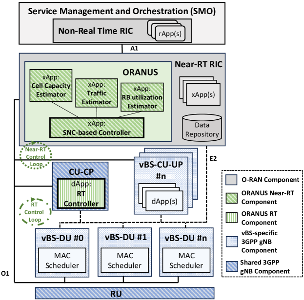
Figure 1: Integration of ORANUS (i.e., green blocks) in the O-RAN architecture.

SNC-based Controller xApp: It obtains the guaranteed amount of RBs $N_{\scriptscriptstyle m}^{\scriptscriptstyle min}$ for each service $m$ $\in\mathcal{M}$, which ensures $\text{P}\left[w>W_{\scriptscriptstyle m}^{\scriptscriptstyle th}\right]<\varepsilon_{\scriptscriptstyle m}$, where $w$ is the packet transmission delay, $W_{\scriptscriptstyle m}^{\scriptscriptstyle th}$ is the delay budget and $\varepsilon_{\scriptscriptstyle m}$ is the target violation probability. To this end, it operates every $T_{\scriptscriptstyle OUT}$ Transmission Time Intervals (TTIs) and exchanges information with the Traffic/Cell Capacity Estimator xApps and the RB utilization Estimator xApp.

Traffic and Cell Capacity Estimator xApps: They analyze each service $m$ $\in\mathcal{M}$ and estimate the incoming traffic demand in terms of the number of bits per TTI. Additionally, they compute arrays of samples, each representing the number of bits that each cell can accommodate for these services in an arbitrary TTI, based on the chosen Modulation and Coding Schemes (MCSs) for packet transmission. To that end, these xApps collect these metrics from each DU via the O1 interface.

RB utilization Estimator xApp: It estimates the Probability Mass Function (PMF) of the RB utilization. To that end, it relies on a Neural Network (NN) based on Mixture Density Network (MDN). It considers the following inputs: (a) the incoming traffic demand in each TTI expressed in bits, (b) the enqueued bits in each TTI and (c) the candidate number of guaranteed RBs for the next $T_{\scriptscriptstyle OUT}$ TTIs. These metrics are available from E2/O1 interfaces.

RT Controller dApp: It operates every TTI and is responsible for ensuring each DU MAC scheduler, one per service $m$ $\in\mathcal{M}$, has available at least $N_{\scriptscriptstyle m}^{\scriptscriptstyle min}$ RBs. Note that $\sum_{\scriptscriptstyle m\in\mathcal{M}}N_{\scriptscriptstyle m}^{\scriptscriptstyle min}\leq N_{\scriptscriptstyle cell}^{\scriptscriptstyle RB}$, where $N_{\scriptscriptstyle cell}^{\scriptscriptstyle RB}$ is the RBs available in the cell. Focusing on a single TTI $t$, if a service $m$ requires a number of RBs $N_{\scriptscriptstyle t}$ such as $N_{\scriptscriptstyle t}<N_{\scriptscriptstyle m}^{\scriptscriptstyle min}$, this dApp will allocate $N_{\scriptscriptstyle t}$ RBs to such service. Otherwise, it will first check if there are any available free RBs, i.e., those RBs that were initially allocated to other services but have not been used in the current TTI. If free RBs are found, the dApp allocates $N_{\scriptscriptstyle m}^{\scriptscriptstyle min}$ plus the available free RBs to the specified service. Additionally, this dApp monitors the transmission buffers to detect traffic anomalies. If so, it temporarily updates $N_{\scriptscriptstyle m}^{\scriptscriptstyle min}$ $\forall m\in\mathcal{M}$ to mitigate the violation probability.

III Latency Model based on SNC

To assess the packet transmission delay, we propose a SNC model. In this section, we first provide some fundamentals on SNC. Then, we describe the steps to compute the delay bound $W$. Finally, we particularize them to our scenario.

III-A Fundamentals on SNC

We use SNC to model the incoming and outgoing traffic of a network node by stochastic arrival and service processes. The arrival process $A(\tau,t)$ represents the cumulative number of bits that arrive at this node, and the service process $S(\tau,t)$ denotes the cumulative number of bits that may be served by this node. Both measured over the time interval $(\tau,t]$.

SNC relies on the Exponentially Bounded Burstiness (EBB) and the Exponentially Bounded Fluctuation (EBF) models [13]. They define an upper bound $\alpha(\tau,t)$, denominated arrival envelope, and a lower bound $\beta(\tau,t)$, denominated service envelope, as Eqs. (1) and (2) show. The parameters $\varepsilon_{A}$ and $\varepsilon_{S}$ are known as the overflow and deficit profiles.

$$\text{P}[A(\tau,t)>\alpha(\tau,t)]\leq\varepsilon_{\scriptscriptstyle A}.$$ (1)

$$\text{P}\left[S(\tau,t)<\beta(\tau,t)\right]\leq\varepsilon_{\scriptscriptstyle S}.$$ (2)

A widely accepted practice in SNC consists of assuming affine functions to define $\alpha(\tau,t)$ and $\beta(\tau,t)$. These functions are defined in Eqs. (3) and (4), where the parameters $\rho_{\scriptscriptstyle A}>0$, $\rho_{\scriptscriptstyle S}>0$ and $b_{\scriptscriptstyle A}\geq 0$, $b_{\scriptscriptstyle S}\geq 0$ are the rate and burst parameters for $\alpha(\tau,t)$ and $\beta(\tau,t)$, respectively. Additionally, $\left[x\right]_{+}$ denotes $\text{max}\{0,x\}$. Finally, $\delta>0$ is a sample path argument considered by the EBB and the EBF models [13].

$$\alpha(\tau,t)=(\rho_{\scriptscriptstyle A}+\delta)[t-\tau]+b_{\scriptscriptstyle A}.$$ (3)

$$\beta(\tau,t)=(\rho_{\scriptscriptstyle S}-\delta)\left[t-\tau-\nicefrac{{b_{\scriptscriptstyle S}}}{{\rho_{\scriptscriptstyle S}}}\right]_{+}.$$ (4)

If we represent $\alpha(\tau,t)$ and $\beta(\tau,t)$ over a $t-\tau$ axis, we can compute the delay bound $W$ as the horizontal deviation between these envelopes. Specifically, this horizontal deviation can be formulated as Eq. (5) shows. Note that this deviation exists when the slope of $\beta(\tau,t)$ is greater than the slope of $\alpha(\tau,t)$. This results in the condition defined in Eq. (6).

$$W=\tfrac{b_{\scriptscriptstyle A}+b_{\scriptscriptstyle S}}{\rho_{\scriptscriptstyle S}-\delta}.$$ (5)

$$\rho_{\scriptscriptstyle S}-\delta>\rho_{\scriptscriptstyle A}+\delta.$$ (6)

III-B SNC Steps to Compute the Delay Bound

Below, we briefly summarize the steps proposed in [13, Sections II.A and II.B] to obtain the arrival envelope, the service envelope and the delay bound.

1. We compute the Moment Generating Functions (MGFs) for the arrival and service processes, i.e., $M_{\scriptscriptstyle A}(\theta)$ and $M_{\scriptscriptstyle S}(\scalebox{0.5}[1.0]{$-$}\theta)$. The MGF of a random process $X$ is defined as $\text{E}\left[e^{\theta X}\right]$ with free parameter $\theta$. Note that searching a lower bound for the service process is equivalent to using the sign $(\scalebox{0.5}[1.0]{$-$})$ for $\theta$.

2. We define upper bounds for the MGFs as Eqs. (7) and (8) show. They are characterized by the rate parameters $\rho_{\scriptscriptstyle A}$ and $\rho_{\scriptscriptstyle S}$, and the burst parameters $\sigma_{\scriptscriptstyle A}$ and $\sigma_{\scriptscriptstyle S}$. Note that $\rho_{\scriptscriptstyle A}$ and $\rho_{\scriptscriptstyle S}$ are the same as the ones defined in Eqs. (3) and (4). If we replace the left side of Eqs. (7) and (8) by the MGFs computed in the previous step, we can obtain the parameters $\rho_{\scriptscriptstyle A}$, $\sigma_{\scriptscriptstyle A}$, $\rho_{\scriptscriptstyle S}$ and $\sigma_{\scriptscriptstyle S}$.

   $$M_{\scriptscriptstyle A}(\theta)\leq\text{exp}\left[\theta\left(\rho_{\scriptscriptstyle A}[t-\tau]+\sigma_{\scriptscriptstyle A}\right)\right].$$ (7)

   $$M_{\scriptscriptstyle S}(\scalebox{0.5}[1.0]{$-$}\theta)\leq\text{exp}\left[\scalebox{0.5}[1.0]{$-$}\theta\left(\rho_{\scriptscriptstyle S}[t-\tau]-\sigma_{\scriptscriptstyle S}\right)\right].$$ (8)

3. The EBB and EBF models defined in Eqs. (1) and (2), and the MGFs are directly connected by the Chernoff bound [14]. Based on it, we can obtain $b_{\scriptscriptstyle A}$ and $b_{\scriptscriptstyle S}$ as Eqs. (9) and (10) shows. Note that a common practice is to equally distribute the target violation probability among the overflow and deficit profiles, i.e., $\varepsilon_{\scriptscriptstyle A}=\varepsilon_{\scriptscriptstyle B}=\varepsilon/2$.

   $$b_{\scriptscriptstyle A}=\sigma_{\scriptscriptstyle A}-\tfrac{1}{\theta}\left[\text{ln}(\varepsilon_{\scriptscriptstyle A})+\text{ln}\left(1-\text{exp}\left[\scalebox{0.5}[1.0]{$-$}\theta\delta\right]\right)\right].$$ (9)

   $$b_{\scriptscriptstyle S}=\sigma_{\scriptscriptstyle S}-\tfrac{1}{\theta}\left[\text{ln}(\varepsilon_{\scriptscriptstyle S})+\text{ln}\left(1-\text{exp}\left[\scalebox{0.5}[1.0]{$-$}\theta\delta\right]\right)\right].$$ (10)

4. Using the previous results in Eq. (5), we can rewrite the delay bound $W$ as Eq. (11) shows. Then, we need to search the values for $\theta$ and $\delta$ that minimize the expression of Eq. (11) to estimate the delay bound.

   $$W=\frac{\sigma_{\scriptscriptstyle A}+\sigma_{\scriptscriptstyle S}-\tfrac{2}{\theta}\left[\text{ln}\left(\frac{\varepsilon}{2}\right)+\text{ln}\left(1-\text{exp}\left[-\theta\delta\right]\right)\right]}{\rho_{\scriptscriptstyle S}-\delta}.$$ (11)

Below, we particularize the arrival process $A(\tau,t)$, the service process $S(\tau,t)$ and the steps to estimate $W$ for a scenario where a cell implements an uRLLC service.

III-C uRLLC Traffic Model

The arrival process $A_{\scriptscriptstyle m}(\tau,t)$ is the cumulative DL traffic of the service $m$, which is defined in Eq. (12). The variable $N_{\scriptscriptstyle slot}(\tau,t)=(t-\tau)/t_{\scriptscriptstyle slot}$ represents the total number of TTIs in $(\tau,t]$, and $t_{\scriptscriptstyle slot}$ denotes the duration of a TTI. The random variable $D_{\scriptscriptstyle m}(i)$ represents the number of bits that arrive to the transmission buffer for service $m$ in the $i$-th TTI.

$$A_{\scriptscriptstyle m}(\tau,t)=\sum_{i=\tau}^{N_{\scriptscriptstyle slot}(\tau,t)}D_{\scriptscriptstyle m}(i).$$ (12)

We assume that the PMF of $D_{\scriptscriptstyle m}(i)$ can be estimated by using samples of the incoming bits per TTI in the last $T_{\scriptscriptstyle OBS}$ TTIs. Specifically, we define the sample vector $\vec{x}_{\scriptscriptstyle D_{\scriptscriptstyle m}}=\{d_{\scriptscriptstyle m,1}^{\scriptscriptstyle in},d_{\scriptscriptstyle m,2}^{\scriptscriptstyle in}\,\ldots\,d_{\scriptscriptstyle m,T_{\scriptscriptstyle OBS}}^{\scriptscriptstyle in}\}$, where $d_{\scriptscriptstyle m,i}^{\scriptscriptstyle in}$ denotes the number of bits that arrive to the transmission buffer in the TTI $i$ for the service $m$. Additionally, $d_{\scriptscriptstyle m,i}^{\scriptscriptstyle in}=\sum_{j=1}^{J_{\scriptscriptstyle m,i}^{\scriptscriptstyle in}}l_{j}$, where $J_{\scriptscriptstyle m,i}^{\scriptscriptstyle in}$ is the number of incoming packets for service $m$ in the TTI $i$ and $l_{\scriptscriptstyle j}$ the size of the packet $j$. Note that the computation of $\vec{x}_{\scriptscriptstyle D_{\scriptscriptstyle m}}$ is a task performed by the Traffic Estimator xApp. With these assumptions, we can compute the MGF for $D_{\scriptscriptstyle m}(i)$:

$$M_{\scriptscriptstyle D_{\scriptscriptstyle m}}(\theta)=\frac{1}{T_{\scriptscriptstyle OBS}}\sum_{i=1}^{T_{\scriptscriptstyle OBS}}\text{exp}\left[\theta d_{\scriptscriptstyle m,i}^{\scriptscriptstyle in}\right].$$ (13)

Considering $M_{\scriptscriptstyle D_{\scriptscriptstyle m}}(\theta)$, we can compute the MGF of the arrival process $A_{\scriptscriptstyle m}(\tau,t)$ as Eq. (14) shows.

$$M_{\scriptscriptstyle A_{\scriptscriptstyle m}}(\theta)=e^{\left[\text{ln}\left(\tfrac{1}{T_{\scriptscriptstyle OBS}}\sum_{i=1}^{T_{\scriptscriptstyle OBS}}\text{exp}\left[\theta d_{\scriptscriptstyle m,i}^{\scriptscriptstyle in}\right]\right)\tfrac{(t-\tau)}{t_{\scriptscriptstyle slot}}\right]}.$$ (14)

Finally, by equaling the left and right sides of Eq. (7), we obtain $\rho_{\scriptscriptstyle A_{\scriptscriptstyle m}}$ as Eq. 15 shows. Note that $\sigma_{\scriptscriptstyle A_{\scriptscriptstyle m}}=0$.

$$\rho_{\scriptscriptstyle A_{\scriptscriptstyle m}}=\frac{\text{ln}\left[\tfrac{1}{T_{\scriptscriptstyle OBS}}\sum_{i=1}^{T_{\scriptscriptstyle OBS}}\text{exp}\left[\theta d_{\scriptscriptstyle m,i}^{\scriptscriptstyle in}\right]\right]}{\theta t_{\scriptscriptstyle slot}}.$$ (15)

III-D Service Model

The service process $S_{\scriptscriptstyle m}(\tau,t)$ represents the accumulated capacity the cell may provide to the service $m$ and can be defined as

$$S_{\scriptscriptstyle m}(\tau,t)=\sum_{i=\tau}^{N_{\scriptscriptstyle slot}(\tau,t)}C_{\scriptscriptstyle m}(i),$$ (16)

where the random variable $C_{\scriptscriptstyle m}(i)$ is the number of bits that may be served by the cell for service $m$ in the TTI $i$.

The negative MGF for $C_{\scriptscriptstyle m}(i)$ is defined in Eq. (17). To that end, we consider the PMF of $C_{\scriptscriptstyle m}(i)$ can be estimated by (a) using samples of the number of bits which may be transmitted in the last $T_{\scriptscriptstyle OBS}$ TTIs and (b) considering the PMF of the RB utilization. The latter captures the dynamics of the RT Controller dApp. Specifically, we consider the sample vectors $\vec{x}_{C_{m},n}=\{c_{\scriptscriptstyle m,1}^{\scriptscriptstyle n,out},c_{\scriptscriptstyle m,2}^{\scriptscriptstyle n,out}\,\ldots\,c_{\scriptscriptstyle m,T_{\scriptscriptstyle m,n}}^{\scriptscriptstyle n,out}\}$ $\forall n\in[0,\;N_{\scriptscriptstyle add}]$ where $c_{\scriptscriptstyle m,i}^{\scriptscriptstyle n,out}$ denotes the number of bits which may be transmitted by the cell for service $m$ in a single TTI, i.e., considering the serving cell uses $n+N_{\scriptscriptstyle m}^{\scriptscriptstyle min}$ RBs for such service. Additionally, $N_{\scriptscriptstyle add}=N_{\scriptscriptstyle cell}^{\scriptscriptstyle RB}-N_{\scriptscriptstyle m}^{\scriptscriptstyle min}$, where $T_{\scriptscriptstyle m,n}$ is the number of samples. Additionally, we consider $\pi_{\scriptscriptstyle m,n}$ as the probability the service $m$ has available $n+N_{\scriptscriptstyle m}^{\scriptscriptstyle min}$ RBs in an arbitrary TTI, conditioned to this service $m$ needs more RBs than $N_{\scriptscriptstyle m}^{\scriptscriptstyle min}$. The computation of $\vec{x}_{\scriptscriptstyle C_{\scriptscriptstyle m},n}$, a task performed by the Cell Capacity Estimator xApp, is detailed in Section IV-A.

$$\begin{split}M_{\scriptscriptstyle C_{\scriptscriptstyle m}}(\scalebox{0.5}[1.0]{$-$}\theta)=\sum_{n=0}^{N_{\scriptscriptstyle add}}\tfrac{\pi_{\scriptscriptstyle m,n}}{T_{\scriptscriptstyle m,n}}\sum_{i=1}^{T_{\scriptscriptstyle m,n}}\text{exp}\left[\scalebox{0.5}[1.0]{$-$}\theta c_{\scriptscriptstyle m,i}^{\scriptscriptstyle n,out}\right].\end{split}$$ (17)

Considering $M_{\scriptscriptstyle C_{\scriptscriptstyle m}}(\scalebox{0.5}[1.0]{$-$}\theta)$, we can compute the negative MGF of the service process $S_{\scriptscriptstyle m}(\tau,t)$ as

$$M_{\scriptscriptstyle S_{\scriptscriptstyle m}}(\scalebox{0.5}[1.0]{$-$}\theta)=e^{\left[\text{ln}\left(\sum_{n=0}^{N_{\scriptscriptstyle add}}\tfrac{\pi_{\scriptscriptstyle m,n}}{T_{\scriptscriptstyle m,n}}\sum_{i=1}^{T_{\scriptscriptstyle m,n}}\text{exp}\left[\scalebox{0.5}[1.0]{$-$}\theta c_{\scriptscriptstyle m,i}^{\scriptscriptstyle n,out}\right]\right)\frac{(t-\tau)}{t_{slot}}\right]}.$$ (18)

Finally, by equaling the left and right sides of Eq. (8), we obtain $\rho_{\scriptscriptstyle S_{\scriptscriptstyle m}}$ as Eq. 19 shows. Note that $\sigma_{\scriptscriptstyle S_{\scriptscriptstyle m}}=0$.

$$\rho_{\scriptscriptstyle S_{\scriptscriptstyle m}}=\frac{-\text{ln}\left[\sum_{n=0}^{N_{\scriptscriptstyle add}}\frac{\pi_{\scriptscriptstyle m,n}}{T_{\scriptscriptstyle m,n}}\sum_{i=1}^{T_{\scriptscriptstyle m,n}}\text{exp}\left[\scalebox{0.5}[1.0]{$-$}\theta c_{\scriptscriptstyle m,i}^{\scriptscriptstyle n,out}\right]\right]}{\theta t_{\scriptscriptstyle slot}}.$$ (19)

III-E Delay Bound Estimation

Using the results from Sections III-C and III-D, we can define $W_{\scriptscriptstyle m}$ as a function of the free parameters $\theta$ and $\delta$, as written in Eq.  20. To estimate $W_{\scriptscriptstyle m}$, we need to solve the following optimization problem.
Problem DELAY_BOUND_CALCULATION:

$$\underset{\theta,\delta}{\text{min}}\quad \frac{2t_{\scriptscriptstyle slot}\left[\text{ln}\left(\frac{\varepsilon_{\scriptscriptstyle m}}{2}\right)+\text{ln}\left(1-\text{exp}\left[\scalebox{0.5}[1.0]{$-$}\theta\delta\right]\right)\right]}{\text{ln}\left[\sum_{n=0}^{N_{\scriptscriptstyle add}}\frac{\pi_{\scriptscriptstyle m,n}}{T_{\scriptscriptstyle m,n}}\sum_{i=1}^{T_{\scriptscriptstyle m,n}}\text{exp}\left[\scalebox{0.5}[1.0]{$-$}\theta c_{\scriptscriptstyle m,i}^{\scriptscriptstyle n,out}\right]\right]+\delta\theta t_{\scriptscriptstyle slot}}.$$ (20)

s.t.: $$\theta,\delta,\rho_{\scriptscriptstyle A_{\scriptscriptstyle m}},\rho_{\scriptscriptstyle S_{\scriptscriptstyle m}}>0,$$ (21)

$$\rho_{\scriptscriptstyle S_{\scriptscriptstyle m}}-\rho_{\scriptscriptstyle A_{\scriptscriptstyle m}}>2\delta.$$ (22)

The previous problem is defined by a non-convex objective function over a non-convex region. It involves the existence of multiple local minimums, thus performing an exhaustive search to find the optimal solution is not computationally tractable. For such reason, we propose the heuristic approach described in Algorithm 1.

1 Inputs: $\varepsilon_{\scriptscriptstyle m}$, $\vec{x}_{\scriptscriptstyle D_{\scriptscriptstyle m}}$, $\vec{x}_{\scriptscriptstyle C_{\scriptscriptstyle m},n}$;

2 Initialization: $\theta_{\scriptscriptstyle z}=1$, $\delta_{\scriptscriptstyle z}$, $y$, $y_{\scriptscriptstyle z}=0$, $stop=False$;

3 while stop == False do

4       Set $\theta_{\scriptscriptstyle z}=\theta_{\scriptscriptstyle z}\Delta$;

5       Compute $\rho_{\scriptscriptstyle A_{\scriptscriptstyle m}}(\theta_{\scriptscriptstyle z})$, $\rho_{\scriptscriptstyle S_{\scriptscriptstyle m}}(\theta_{z})$ [See Eqs. (15) and (19)];

6       if  $\rho_{\scriptscriptstyle S_{\scriptscriptstyle m}}(\theta_{\scriptscriptstyle z})>\rho_{\scriptscriptstyle A_{\scriptscriptstyle m}}(\theta_{\scriptscriptstyle z})$ then

7             Compute $\delta_{\scriptscriptstyle z}=\left(\rho_{\scriptscriptstyle S_{\scriptscriptstyle m}}(\theta_{\scriptscriptstyle z})-\rho_{\scriptscriptstyle A_{\scriptscriptstyle m}}(\theta_{\scriptscriptstyle z})\right)/2$;

8             Compute $y_{\scriptscriptstyle z}=\theta_{\scriptscriptstyle z}\delta_{\scriptscriptstyle z}$;

9             if $y_{\scriptscriptstyle z}>y$  then

10                   Set $y=y_{\scriptscriptstyle z}$, $\theta_{\scriptscriptstyle opt}=\theta_{\scriptscriptstyle z}$, $\delta_{\scriptscriptstyle opt}=\delta_{\scriptscriptstyle z}$;

11                   Compute $W_{\scriptscriptstyle m}(\theta_{\scriptscriptstyle opt},\delta_{\scriptscriptstyle opt})$. See Eq. (20);

12                  

13            else

14                   $stop=True$;

15                  

16             end if

17            

18       end if

19      

20 end while

21return: $\theta_{opt}$, $\delta_{opt}$, $W_{m}$;

Algorithm 1 Calculation Delay Bound $W_{m}$

This algorithm takes as inputs the target violation probability $\varepsilon_{\scriptscriptstyle m}$ for service $m$ and the sample vectors $\vec{x}_{\scriptscriptstyle D_{\scriptscriptstyle m}}$ and $\vec{x}_{\scriptscriptstyle C_{\scriptscriptstyle m},n}$, and iteratively searches the values of $\theta$ and $\delta$ which minimize Eq. (20), i.e., $\theta_{\scriptscriptstyle opt}$ and $\delta_{\scriptscriptstyle opt}$. We experimentally observed the rate parameter $\rho_{\scriptscriptstyle S_{\scriptscriptstyle m}}$, i.e., Eq. (19), increases when $\theta$ decreases. Note that a greater $\rho_{\scriptscriptstyle S_{\scriptscriptstyle m}}$ reduces the delay bound $W_{\scriptscriptstyle m}$ as Eq. (11) shows. Additionally, the numerator of Eq. (20) is monotonically increasing with the product $\theta\delta$. Based on that, Algorithm 1 first reduces the value of $\theta_{\scriptscriptstyle z}$, i.e., the candidate value of $\theta_{\scriptscriptstyle opt}$, in each iteration (step 4). Such reduction is performed by the parameter $\Delta\in(0,1)$. Refining $\Delta$ towards 1 enhances the granularity of locating $W_{\scriptscriptstyle m}$, albeit at the cost of requiring a larger number of iterations. Then, Algorithm 1 computes the rate parameters $\rho_{\scriptscriptstyle A_{\scriptscriptstyle m}}(\theta_{\scriptscriptstyle z})$ and $\rho_{\scriptscriptstyle S_{\scriptscriptstyle m}}(\theta_{\scriptscriptstyle z})$ (step 5). If $\rho_{\scriptscriptstyle S_{\scriptscriptstyle m}}(\theta_{\scriptscriptstyle z})>\rho_{\scriptscriptstyle A_{\scriptscriptstyle m}}(\theta_{\scriptscriptstyle z})$, i.e., from constraints (21)-(22), the algorithm computes the candidate value of $\delta$, i.e., $\delta_{\scriptscriptstyle z}$ (step 7). If the product $\theta_{\scriptscriptstyle z}\delta_{\scriptscriptstyle z}$ (step 8) improves the product computed in the previous iteration, $W_{\scriptscriptstyle m}$ gets updated. In such a case, the algorithm sets $\theta_{\scriptscriptstyle opt}$ and $\delta_{\scriptscriptstyle opt}$ (step 10), computes $W_{\scriptscriptstyle m}$ (step 11), and tries another iteration to reduce $W_{\scriptscriptstyle m}$. When the product $\theta_{\scriptscriptstyle z}\delta_{\scriptscriptstyle z}$ does not improve with respect to the result of the previous iteration, the algorithm stops (step 13) and considers the latter as the optimal solution.

IV Control Loops of ORANUS

In this section, we explain how ORANUS performs the near-RT and RT control loops. Specifically, we first describe how the samples of the cell capacity are computed as well as the estimation of the probabilities $\pi_{\scriptscriptstyle m,n}$. Then, we explain how the SNC-based Controller xApp decides $N_{\scriptscriptstyle m}^{\scriptscriptstyle min}$ $\forall m\in\mathcal{M}$ for the near-RT control loop. Finally, we describe how the RT Controller dApp mitigates the violation probability.

IV-A Computation of the Cell Capacity Samples

The Cell Capacity Estimator xApp performs the following steps to obtain a sample $c_{\scriptscriptstyle m,i}^{\scriptscriptstyle n,out}\in\vec{x}_{\scriptscriptstyle C_{\scriptscriptstyle m},n}$.

1. For each transmitted packet $j$, it considers (a) the packet size $l_{\scriptscriptstyle j}$, and (b) the amount of RBs required to transmit it, i.e., $N_{\scriptscriptstyle pkt,j}$. Note that we are assuming that a unique MCS value is adopted to transmit each packet. It means this xApp can compute the number of bits transmitted per RB as $c_{\scriptscriptstyle RB,j}=l_{\scriptscriptstyle j}/N_{\scriptscriptstyle pkt,j}$. Based on that, it defines a vector $\vec{x}_{\scriptscriptstyle pkt,j}=\{c_{\scriptscriptstyle RB,j},c_{\scriptscriptstyle RB,j}\,\ldots,c_{\scriptscriptstyle RB,j}\}$, where the element $c_{\scriptscriptstyle RB,j}$ is repeated $N_{\scriptscriptstyle pkt,j}$ times.

2. Performing the previous step for all the transmitted packets, this xApp obtains a set of vectors $\vec{x}_{\scriptscriptstyle pkt,j}$ $\forall j\in\mathcal{J}_{\scriptscriptstyle OBS}$, where $\mathcal{J}_{\scriptscriptstyle OBS}$ denotes the set of packets transmitted in the last $T_{\scriptscriptstyle OBS}$ TTIs. Based on that, this xApp defines $\vec{x}_{\scriptscriptstyle con}=\{\vec{x}_{\scriptscriptstyle pkt,1},\vec{x}_{\scriptscriptstyle pkt,2}\,\ldots\vec{x}_{\scriptscriptstyle pkt,|\mathcal{J}_{OBS}|}\}$ as a vector which concatenates each measured vector $\vec{x}_{\scriptscriptstyle pkt,j}$.

3. Based on $\vec{x}_{\scriptscriptstyle con}$, this xApp groups its samples in set of $N_{\scriptscriptstyle m,n}^{\scriptscriptstyle set}=n+N_{\scriptscriptstyle m}^{\scriptscriptstyle min}$ consecutive samples. In turn, each group of $N_{\scriptscriptstyle m,n}^{\scriptscriptstyle set}$ consecutive samples defines a vector $\vec{x}_{\scriptscriptstyle m,i}^{\scriptscriptstyle n,out}$, where $i\in[1,T_{\scriptscriptstyle m,n}]$ represents the i-th vector. We define $T_{\scriptscriptstyle m,n}$ as the total number of built vectors. Note we have one vector $\vec{x}_{\scriptscriptstyle m,i}^{\scriptscriptstyle n,out}$ per sample $c_{\scriptscriptstyle m,i}^{\scriptscriptstyle n,out}$, i.e., see Eq. (17).

4. Finally, this xApp obtains the sample $c_{\scriptscriptstyle m,i}^{\scriptscriptstyle n,out}$ as the sum of all the elements of the vector $\vec{x}_{\scriptscriptstyle m,i}^{\scriptscriptstyle n,out}$, i.e., $c_{\scriptscriptstyle m,i}^{\scriptscriptstyle n,out}=\sum_{z=1}^{N_{\scriptscriptstyle m,n}^{\scriptscriptstyle set}}\vec{x}_{\scriptscriptstyle m,i}^{\scriptscriptstyle n,out}\{z\}$.

IV-B Mixture Density Networks for estimating the RB utilization

The SNC-based Controller xApp relies on a MDN, which is a NN architecture designed to model probability distributions [15], to estimate $\pi_{m,n}$. Typically, the NN’s output layer produces a single value that represents the predicted outcome. In an MDN, the output layer generates one or more parameterized mixture models, each being a weighted combination of several component distributions. In this paper, we consider $|\mathcal{M}|$ Gaussian Mixture Models (GMMs), one per service. It is proven the GMM accurately approximate any arbitrary distribution in the context of wireless networks [16, 17, 18]. Specifically, $\pi_{\scriptscriptstyle m,n}$ may not follow a single known statistical distribution and perhaps more importantly, it may also change over time. The GMM is described by the equation depicted in Fig. 2, where $K_{\scriptscriptstyle m}$ denotes the number of Gaussian distributions. In turn, the $k$-th distribution is characterized by the weight $w_{\scriptscriptstyle k,m}$, the mean $\mu_{\scriptscriptstyle k,m}$ and the standard deviation $\sigma_{\scriptscriptstyle k,m}$. Note that $\sum_{k=1}^{K_{\scriptscriptstyle m}}w_{\scriptscriptstyle k,m}=1$.

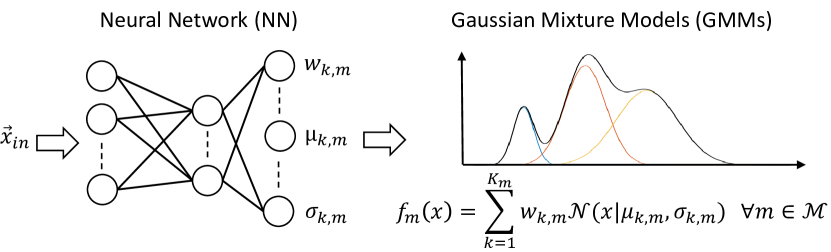
Figure 2: Overview of the considered Mixture Density Network (MDN).

The considered MDN is summarized in Fig. 2. The inputs parameters $\vec{x}_{\scriptscriptstyle in}$ are: (a) the RB utilization for each service, and (b) the 25th, 50th and 75th percentiles of incoming and enqueued bits. All of them measured in the last $T_{\scriptscriptstyle OUT}$ TTIs for each service $m\in\mathcal{M}$. Additionally, the MDN considers as input the target number of guaranteed RBs for each service $m\in\mathcal{M}$ in the next $T_{\scriptscriptstyle OUT}$ TTIs. Based on them, the MDN provides an estimation of the parameters $w_{\scriptscriptstyle k,m}$, $\mu_{\scriptscriptstyle k,m}$ and $\sigma_{k,m}$. Finally, we compute the $\pi_{\scriptscriptstyle m,n}$ as Eq. 23 shows. Specifically, we split the GMM into $N_{\scriptscriptstyle add}$ regions (i.e., see Section III-D) and compute $\pi_{\scriptscriptstyle m,n}$ as the probability of being in the $n$-th region.

$$\pi_{\scriptscriptstyle m,n}=\sum_{k=1}^{K_{\scriptscriptstyle m}}\int_{n-0.5}^{n+0.5}w_{\scriptscriptstyle k,m}\mathcal{N}\left(x|\mu_{\scriptscriptstyle k,m},\sigma_{\scriptscriptstyle k,m}\right)dx.$$ (23)

IV-C Near-RT Control Loop

The SNC-based Controller xApp aims to determine $N_{\scriptscriptstyle m}^{\scriptscriptstyle min}$ $\forall m\in\mathcal{M}$ such as the delay bound $W_{\scriptscriptstyle m}$ is as close as possible (or even below) to the target delay budget $W_{\scriptscriptstyle m}^{th}$, given the target violation probability $\varepsilon_{\scriptscriptstyle m}$. To that end, we formulate the problem ORCHESTRATION_URLLC_SERVICES. It consists of minimizing the maximum ratio $W_{\scriptscriptstyle m}/W_{\scriptscriptstyle m}^{\scriptscriptstyle th}$, i.e., considering $|\mathcal{M}|$ services, as Eq. (24) shows. This problem is constrained by Eq. (25), which ensures the sum of the amount of guaranteed RBs of all the services must be equal or less than the available RBs.
Problem ORCHESTRATION_URLLC_SERVICES:

$$\underset{N_{\scriptscriptstyle m}^{\scriptscriptstyle min}}{\text{min.}}\quad g(\vec{W})=\text{max}\left\{\nicefrac{{W_{\scriptscriptstyle 1}}}{{W_{\scriptscriptstyle 1}^{\scriptscriptstyle th}}},\ldots,\nicefrac{{W_{\scriptscriptstyle|\mathcal{M}|}}}{{W_{\scriptscriptstyle|\mathcal{M}|}^{\scriptscriptstyle th}}}\right\}.$$ (24)

s.t.: $$\sum_{m=1}^{|\mathcal{M}|}N_{\scriptscriptstyle m}^{\scriptscriptstyle min}\leq N_{\scriptscriptstyle cell}^{\scriptscriptstyle RB}.$$ (25)

The objective function $g(\vec{W})$ depends on the computation of $W_{\scriptscriptstyle m}$ $\forall m\in\mathcal{M}$. Specifically, when a specific value of $N_{\scriptscriptstyle m}^{\scriptscriptstyle min}$ is considered for each service, $|\mathcal{M}|$ sub-problems as DELAY_BOUND_CALCULATION, i.e., see Eqs. (20)-(22), must be solved. Since each sub-problem requires the optimization of a non-convex function over a non-convex region, we propose Algorithm 2 to solve this problem.

1 Inputs: $W_{\scriptscriptstyle m}^{\scriptscriptstyle th}$, $\varepsilon_{\scriptscriptstyle m}$, $\vec{x}_{\scriptscriptstyle D_{\scriptscriptstyle m}}$, $\vec{x}_{\scriptscriptstyle C_{\scriptscriptstyle m},n}$;

2 Initialization: $N_{\scriptscriptstyle m,z}^{\scriptscriptstyle min}=\lfloor N_{\scriptscriptstyle cell}^{\scriptscriptstyle RB}/|\mathcal{M}|\rfloor$, $W_{\scriptscriptstyle m}=\infty$, $W_{\scriptscriptstyle m,z}=\infty$ $stop=False$;

3 while stop == False do

4       Estimate $\pi_{\scriptscriptstyle m,n}$ $\forall m\in\mathcal{M}$ $\forall n\in[0,N_{\scriptscriptstyle add}]$ [Section IV-B];

5       Estimate $W_{\scriptscriptstyle m,z}$ $\forall m\in\mathcal{M}$ [See Algorithm 1];

6       Evaluate $g(\vec{W}_{\scriptscriptstyle z})$ and $g(\vec{W})$ [See Eq. (24)];

7       if $g(\vec{W}_{\scriptscriptstyle z})<g(\vec{W})$  then

8             Update $N_{\scriptscriptstyle m}^{\scriptscriptstyle min}=N_{\scriptscriptstyle m,z}^{\scriptscriptstyle min}$; $W_{\scriptscriptstyle m}=W_{\scriptscriptstyle m,z}$ $\forall m\in\mathcal{M}$;

9             Select $m^{\scriptscriptstyle\prime}|\nicefrac{{W_{\scriptscriptstyle m^{\scriptscriptstyle\prime}}}}{{W_{\scriptscriptstyle m^{\scriptscriptstyle\prime}}^{\scriptscriptstyle th}}}\geq\nicefrac{{W_{\scriptscriptstyle m}}}{{W_{\scriptscriptstyle m}^{\scriptscriptstyle th}}}$ $\forall m\in\mathcal{M}\setminus\{m^{\scriptscriptstyle\prime}\}$;

10             Select $m^{\scriptscriptstyle\prime\prime}|\nicefrac{{W_{\scriptscriptstyle m^{\scriptscriptstyle\prime\prime}}}}{{W_{\scriptscriptstyle m^{\scriptscriptstyle\prime\prime}}^{\scriptscriptstyle th}}}\leq\nicefrac{{W_{\scriptscriptstyle m}}}{{W_{\scriptscriptstyle m}^{\scriptscriptstyle th}}}$ $\forall m\in\mathcal{M}\setminus\{m^{\scriptscriptstyle\prime\prime}\}$;

11             Compute $N_{\scriptscriptstyle m^{\scriptscriptstyle\prime},z}^{min}=N_{\scriptscriptstyle m^{\scriptscriptstyle\prime}}^{min}+1$; $N_{\scriptscriptstyle m^{\scriptscriptstyle\prime\prime},z}^{\scriptscriptstyle min}=N_{\scriptscriptstyle m^{\scriptscriptstyle\prime\prime}}^{min}-1$;

12            

13      else

14             $stop=True$;

15            

16       end if

17      

18 end while

19return: $N_{m}^{min}$, $W_{m}$;

Algorithm 2 Near-RT RB allocation

This algorithm considers as inputs the target delay budget $W_{\scriptscriptstyle m}^{\scriptscriptstyle th}$, the target violation probability $\varepsilon_{\scriptscriptstyle m}$ and the sample vectors $\vec{x}_{\scriptscriptstyle D_{\scriptscriptstyle m}}$, $\vec{x}_{\scriptscriptstyle C_{\scriptscriptstyle m},n}$. Additionally, it considers as starting point an equal distribution of the available RBs among the services, i.e., $N_{\scriptscriptstyle m,z}^{\scriptscriptstyle min}=\lfloor N_{\scriptscriptstyle cell}^{\scriptscriptstyle RB}/|\mathcal{M}|\rfloor$. Based on them, Algorithm 2 starts an iterative procedure to get $N_{\scriptscriptstyle m}^{\scriptscriptstyle min}$ $\forall m\in\mathcal{M}$. In each iteration, considering $N_{\scriptscriptstyle m,z}^{\scriptscriptstyle min}$ guaranteed RBs for each service, it first estimates $\pi_{\scriptscriptstyle m,n}$ using the MDN described in Section IV-B (step 4). Then, it uses the SNC-based model (see Section III-E) to estimate the delay bound $W_{\scriptscriptstyle m,z}$ for the target $N_{\scriptscriptstyle m,z}^{\scriptscriptstyle min}$ (step 5). Then, it evaluates the objective function, i.e., Eq. (24), considering $W_{\scriptscriptstyle m,z}$ and $W_{\scriptscriptstyle m}$ (step 6). Based on that, it checks if the objective function has been reduced with respect to the previous iteration (step 7). If so, this algorithm updates the new values for $N_{\scriptscriptstyle m}^{\scriptscriptstyle min}$ and $W_{\scriptscriptstyle m}$ (step 8) and tries to reduce the objective function. To that end, it selects the service $m^{\scriptscriptstyle\prime}$ with the best ratio $W_{m^{\scriptscriptstyle\prime}}/W_{\scriptscriptstyle m^{\scriptscriptstyle\prime}}^{\scriptscriptstyle th}$ and the service $m^{\scriptscriptstyle\prime\prime}$ with the worst ratio $W_{m^{\scriptscriptstyle\prime\prime}}/W_{\scriptscriptstyle m^{\scriptscriptstyle\prime\prime}}^{\scriptscriptstyle th}$ (steps 9-10). Next, Algorithm 2 takes one guaranteed RB from the service $m^{\scriptscriptstyle\prime\prime}$ to be assigned to the service $m^{\scriptscriptstyle\prime}$ (step 11). Finally, a new iteration of the algorithm starts if $N_{\scriptscriptstyle m,z}^{\scriptscriptstyle min}$ $\forall m\in\mathcal{M}$ improves the objective function. Conversely, the iterative procedure ends if the objective function can not be further improved (step 13).

IV-D RT Control Loop

Every $T_{\scriptscriptstyle OUT}$ TTIs, the RT Controller dApp receives the new value of $N_{\scriptscriptstyle m}^{\scriptscriptstyle min}$ $\forall m\in\mathcal{M}$ from the SNC-based Controller xApp. Based on them, the RT Controller dApp operates at each TTI as follows. First, it tries to drain the transmission queue of each service $m$ by using $N_{\scriptscriptstyle m}^{\scriptscriptstyle min}$ RBs. After, a subset $\mathcal{M}^{\scriptscriptstyle\prime}\subset\mathcal{M}$ of services will have drained their queues, while the remaining $\mathcal{M}^{\scriptscriptstyle\prime\prime}=\mathcal{M}-\mathcal{M}^{\scriptscriptstyle\prime}$ services may still have pending transmissions. Assuming the $|\mathcal{M}^{\scriptscriptstyle\prime}|$ services have not fully consumed $N_{\scriptscriptstyle fr}$ RBs, such spare resources can be used to for the remaining $|\mathcal{M}^{\scriptscriptstyle\prime\prime}|$ services. Specifically, the $N_{\scriptscriptstyle fr}$ RBs will be allocated among the $|\mathcal{M}^{\scriptscriptstyle\prime\prime}|$ services following the Earliest Deadline First (EDF) discipline [19] since it minimizes the number of packets whose transmission delay is above the target delay budget. Note that EDF does not consider the violation probability [20]. For this reason, the RT Controller dApp combines EDF with the establishment of guaranteed RBs per service. Since the latter are decided by the SNC-based Controller xApp, our framework ensures $\text{P}\left[w>W_{\scriptscriptstyle m}\right]\leq\varepsilon_{\scriptscriptstyle m}$ $\forall m\in\mathcal{M}$ as long as the traffic and channel conditions do not change with respect to the samples $\vec{x}_{\scriptscriptstyle D_{\scriptscriptstyle m}}$, $\vec{x}_{\scriptscriptstyle C_{\scriptscriptstyle m},n}$.

If the traffic and/or channel conditions change, the probability the packet transmission delay $w$ is greater than the estimated delay budget $W_{\scriptscriptstyle m}$ may be greater than the violation probability, i.e., $\text{P}\left[w>W_{\scriptscriptstyle m}\right]\geq\varepsilon_{\scriptscriptstyle m}$. To avoid it whenever possible, the RT Controller dApp executes Algorithm 3.

1 Inputs: $N_{\scriptscriptstyle m}^{\scriptscriptstyle min}$, $Q_{\scriptscriptstyle T,m}^{\scriptscriptstyle U}$, $Q_{\scriptscriptstyle T,m}^{\scriptscriptstyle L}$, $\vec{s}_{\scriptscriptstyle i-1}$;

2 Compute $q_{\scriptscriptstyle i,m}$ $\forall m\in\mathcal{M}$;

3 Update states $\vec{s}_{\scriptscriptstyle i}$ and $N_{\scriptscriptstyle m,i}^{\scriptscriptstyle req}$ according to Fig. 3;

4

5$\vec{v}_{\scriptscriptstyle d}=\big{\{}m^{\scriptscriptstyle\prime}\big{\}}$ $\forall m^{\scriptscriptstyle\prime}$ $|\vec{s}_{\scriptscriptstyle i}\{m^{\scriptscriptstyle\prime}\}=A$ ;

6 $\vec{v}_{\scriptscriptstyle b}=\big{\{}m^{\scriptscriptstyle\prime\prime}\big{\}}$ $\forall m^{\scriptscriptstyle\prime\prime}$ $|\vec{s}_{\scriptscriptstyle i}\{m^{\scriptscriptstyle\prime\prime}\}=B\cup C$;

7 if $\vec{v}_{d}\neq\emptyset$ then

8       Set $N_{\scriptscriptstyle ite}=\sum_{m^{\scriptscriptstyle\prime\prime}}N_{m^{\scriptscriptstyle\prime\prime},i}^{\scriptscriptstyle req}$ and $N_{\scriptscriptstyle m,i}^{\scriptscriptstyle min}=N_{\scriptscriptstyle m}^{\scriptscriptstyle min}$ $\forall m\in\mathcal{M}$;

9       Set $j_{\scriptscriptstyle d}=0$ and $j_{\scriptscriptstyle b}=0$;

10       for $u$ from 1 to $N_{ite}$ do

11             Determine $n^{\scriptscriptstyle\prime}=\vec{v_{\scriptscriptstyle d}}\{j\}$ and $n^{\scriptscriptstyle\prime\prime}=\vec{v_{\scriptscriptstyle b}}\{j\}$;

12             Update $N_{\scriptscriptstyle n^{\scriptscriptstyle\prime},i}^{\scriptscriptstyle min}=N_{\scriptscriptstyle n^{\scriptscriptstyle\prime},i}^{\scriptscriptstyle min}-1$; $N_{\scriptscriptstyle n^{\scriptscriptstyle\prime\prime},i}^{\scriptscriptstyle min}=N_{\scriptscriptstyle n^{\scriptscriptstyle\prime\prime},i}^{\scriptscriptstyle min}+1$;

13             Update $j_{\scriptscriptstyle d}=j_{\scriptscriptstyle d}+1$ and $j_{\scriptscriptstyle b}=j_{\scriptscriptstyle b}+1$;

14             if $j_{\scriptscriptstyle d}==|\vec{v}_{\scriptscriptstyle d}|$ then

15                   $j_{\scriptscriptstyle d}=0$

16             end if

17            if $j_{\scriptscriptstyle b}==|\vec{v}_{\scriptscriptstyle b}|$ then

18                   $j_{\scriptscriptstyle b}=0$

19             end if

20            

21       end for

22      

23 end if

24return: $N_{\scriptscriptstyle m,i}^{\scriptscriptstyle min}$, $N_{\scriptscriptstyle m,i}^{\scriptscriptstyle req}$;

Algorithm 3 Mitigating $w>W_{\scriptscriptstyle m}^{\scriptscriptstyle th}$ at TTI $i$

This algorithm monitors the waiting time of the first packet of each service in the transmission queue. Then, if the waiting time is close to the delay budget, the algorithm increases (if possible) the amount of guaranteed RBs for the corresponding service. To this end, Algorithm 3 relies on a finite-state machine of three states $\big{\{}A,B,C\big{\}}$ based on two thresholds $Q_{\scriptscriptstyle T,m}^{\scriptscriptstyle U}$ and $Q_{\scriptscriptstyle T,m}^{\scriptscriptstyle L}$. The threshold $Q_{\scriptscriptstyle T,m}^{\scriptscriptstyle U}=\eta Q_{\scriptscriptstyle T,m}$ indicates the waiting time of a packet is close to the delay budget, whereas $Q_{\scriptscriptstyle T,m}^{\scriptscriptstyle L}=\tau Q_{\scriptscriptstyle T,m}$ indicates the waiting time is far to the delay budget. The parameter $Q_{\scriptscriptstyle T,m}=\lfloor W_{\scriptscriptstyle m}^{\scriptscriptstyle th}/t_{\scriptscriptstyle slot}\rfloor$ is the maximum number of TTIs that a packet can wait in the queue before crossing the delay budget. Additionally, $Q_{\scriptscriptstyle T,m}^{\scriptscriptstyle U}>Q_{\scriptscriptstyle T,m}^{\scriptscriptstyle L}$. Note that $\eta\in(0,1]$ and $\tau\in(0,1]$ can be tuned by the MNO. Regarding the states, the state $A$ indicates the RT Controller dApp allocates to the service $m$ the amount of guaranteed RBs decided by the SNC-based Controller dApp, i.e., $N_{\scriptscriptstyle m,i}^{\scriptscriptstyle min}=N_{\scriptscriptstyle m}^{\scriptscriptstyle min}$. Note that we define $N_{\scriptscriptstyle m,i}^{\scriptscriptstyle min}$ as the amount of guaranteed RBs decided by the RT Controller dApp in the TTI $i$. The state $B$ indicates the waiting time of the first packet of service $m$ is very close to the delay budget, thus the RT Controller dApp may increase the amount of guaranteed RBs for such service. Specifically, it may increase $N_{\scriptscriptstyle m,i}^{\scriptscriptstyle req}$ RBs. In state $B$, $N_{m,i}^{\scriptscriptstyle req}$ increases by one RB with respect to the previous TTI. The state $C$ indicates the waiting time of the first packet is lower than in state $B$, but not enough to go back to $N_{\scriptscriptstyle m,i}^{\scriptscriptstyle min}=N_{\scriptscriptstyle m}^{\scriptscriptstyle min}$. In such case, Algorithm 3 keeps the same value of $N_{\scriptscriptstyle m,i}^{\scriptscriptstyle req}$ with respect to the previous TTI. In Fig. 3 we summarize the possible transitions among states. Considering such transitions, we define $\vec{s}_{\scriptscriptstyle i}$ as a vector containing the state for each service at TTI $i$.

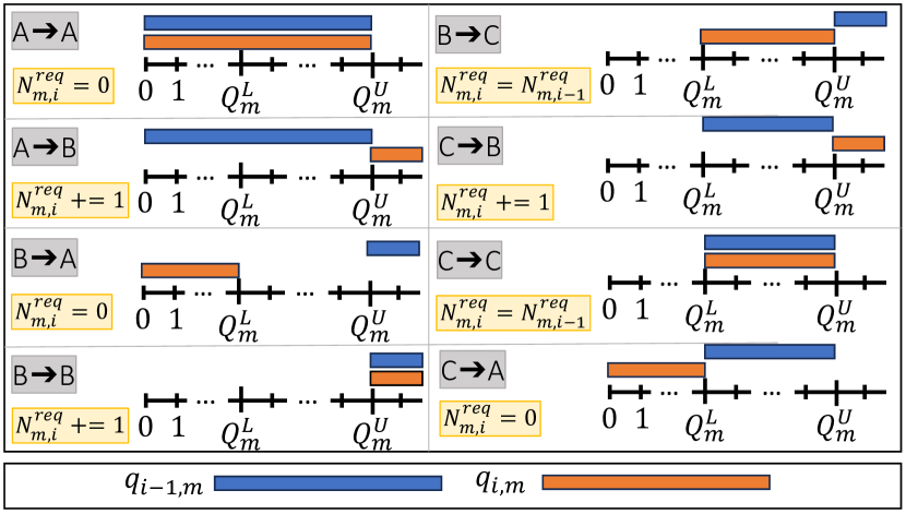
Figure 3: Transitions of the finite-state machine to control the RB allocation for service $m$.

Based on $N_{\scriptscriptstyle m}^{\scriptscriptstyle min}$, $Q_{\scriptscriptstyle T,m}^{\scriptscriptstyle L}$, $Q_{\scriptscriptstyle T,m}^{\scriptscriptstyle U}$ and $\vec{s}_{\scriptscriptstyle i-1}$, Algorithm 3 initially computes the state of the first packet of each service as $q_{\scriptscriptstyle i,m}=w_{\scriptscriptstyle m}^{\scriptscriptstyle pkt}/t_{\scriptscriptstyle slot}$ (step 2). Note that $w_{\scriptscriptstyle m}^{\scriptscriptstyle pkt}$ is the waiting time of such a packet. Then, it updates the states $\vec{s}_{\scriptscriptstyle i}$ and $N_{\scriptscriptstyle m,i}^{\scriptscriptstyle req}$ according to the transitions depicted in Fig. 3 (step 3). Later, Algorithm 3 needs to check if the amount of RBs defined in $N_{\scriptscriptstyle m,i}^{\scriptscriptstyle req}$ can be allocated, in addition to $N_{\scriptscriptstyle m}^{\scriptscriptstyle min}$, to the corresponding services. The policy considered by Algorithm 3 is that only the services whose state is $A$ can donate RBs to those which require more RBs. Considering this policy, Algorithm 3 iteratively re-allocates the amount of guarantees RBs from services in state $A$ to services in states $B$ or $C$ (steps 4-20).

V Performance Evaluation

We perform an exhaustive simulation campaign to validate ORANUS, and evaluate its performances through a Python-based simulator running on a computing platform with $16$ GB RAM and a quad-core Intel Core i7-7700HQ @ 2.80 GHz. The simulator considers a single cell using an Orthogonal Frequency-Division Multiple Access (OFDMA) scheme with $N_{\scriptscriptstyle cell}^{\scriptscriptstyle RB}\in[50,100]$ RBs and $t_{\scriptscriptstyle slot}$ = 1 ms. Regarding the incoming traffic and cell capacity of each uRLLC service, we consider realistic traces collected over an operational RAN using the FALCON tool [21]. The tool allows decoding the Physical Downlink Control Channel (PDCCH) of a base station, revealing the number of active users and their scheduled resources. We make the traces public to foster research on the topic and favor reproducibility. Fig. 4 depicts the incoming bits per TTI measured by FALCON, as well as the corresponding PMF (i.e., upper plots). To emulate the incoming traffic of three different uRLLC services, we order the active User Equipments (UEs) and split them into equally-sized groups, considering their aggregated traffic demand. The resulting PMFs are also displayed in Fig. 4 (lower plots).

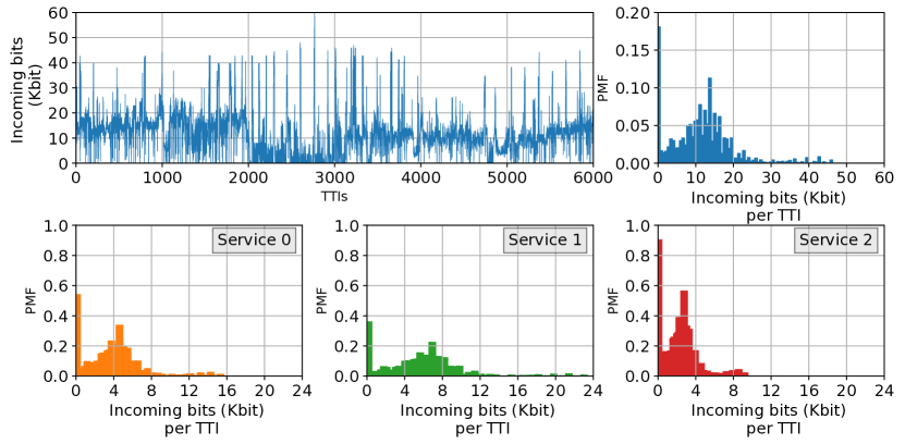
Figure 4: PMFs of incoming bits from FALCON traces.

For these services, we set a delay budget $W_{\scriptscriptstyle m}^{\scriptscriptstyle th}=\big{\{}5,10,15\big{\}}$ ms and target violation probability $\varepsilon_{\scriptscriptstyle m}=\big{\{}10^{-5},10^{-4},10^{-3}\big{\}}$ [22, 23, 24].

V-A Validation of SNC model

In the first experiment, we consider a cell hosting a single service $m$ with the incoming traffic measured by FALCON (i.e., blue plots in Fig. 4). Assuming a target violation probability $\varepsilon_{\scriptscriptstyle m}=10^{-3}$, we compute the delay bound $W_{\scriptscriptstyle m}^{\scriptscriptstyle mod}$ using the proposed SNC model and compare it with the real bound $W_{\scriptscriptstyle m}^{\scriptscriptstyle sim}$ obtained by simulation while the SNC-based Controller xApp (a) allocates $N_{\scriptscriptstyle m}^{\scriptscriptstyle min}\in\left[50,100\right]$ RBs for such service, and (b) uses $T_{\scriptscriptstyle OBS}\in\big{\{}1,2,3,4,5,6\big{\}}\cdot 1000$ TTIs to obtain $\vec{x}_{\scriptscriptstyle D_{m}}$ and $\vec{x}_{\scriptscriptstyle C_{\scriptscriptstyle m},n}$.

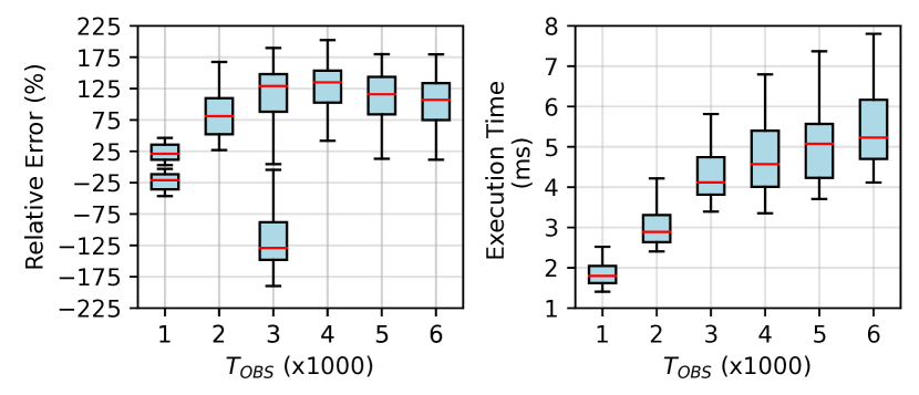
Figure 5: Validation SNC-based model.

The results are depicted in Fig. 5. On the left side, the box-and-whisker plot represents the distribution of the relative error $\epsilon_{\scriptscriptstyle r}=(W_{\scriptscriptstyle m}^{\scriptscriptstyle mod}-W_{\scriptscriptstyle m}^{\scriptscriptstyle sim})/W_{\scriptscriptstyle m}^{\scriptscriptstyle sim}\cdot 100$ when considering a variable $T_{\scriptscriptstyle OBS}$. Note that we have used two boxes in those scenarios which present negative relative errors. Specifically, each box gathers either the positive relative errors or the negative relative errors. We can notice the mean relative error is always below 150%. Such value may appear large at first, but is in fact acceptable, as the goal of our SNC-based model is to accommodate complex arrival and service processes at the expense of obtaining an exact match between the model and simulator results. Instead, SNC promises an upper and conservative estimation of $W_{\scriptscriptstyle m}$, which is of key importance to meet uRLLC services’ requirements in real scenarios.

From the same picture, we can observe negative values for $\epsilon_{\scriptscriptstyle r}$ when $T_{\scriptscriptstyle OBS}\leq 3000$ TTIs. This is due to the insufficient number of samples in vectors $\vec{x}_{\scriptscriptstyle D_{\scriptscriptstyle m}}$ and $\vec{x}_{\scriptscriptstyle C_{\scriptscriptstyle m},n}$, which are not enough to capture the PMFs for the incoming traffic and cell capacity for the corresponding service. In our settings, the proposed SNC model needs at least a period of $T_{\scriptscriptstyle OBS}=4000$ TTIs to effectively capture such PMFs and provide a meaningful upper estimation of the delay bound.

On the right-hand side, the plot shows the execution time distribution of the proposed SNC model. The time monotonically increases with $T_{\scriptscriptstyle OBS}$ as more samples need to be considered in Eqs. (15), (19) and (20). For the considered scenarios, the average execution time is below 6 ms, making the proposed model suitable for determining the amount of guaranteed RBs for uRLLC services in a near-RT scale.

V-B Validation of MDN

In Section IV-B, we propose a neural network model to expedite the estimation of $\pi_{m,n}$. To validate the proposed MDN approach, we split the FALCON dataset according to a 70/30 ratio for the purposes of training and testing, respectively. Furthermore, the number of active UEs are grouped in a uniform way to form the traffic demand of each service. In our implementation, the MDN accounts for a $4$-staged network, characterized by $256$, $256$, $64$, and $3\cdot K_{\scriptscriptstyle m}\cdot|\mathcal{M}|$ neurons, respectively. We empirically select the Rectified Linear Units (ReLu) as activation function to overcome the vanishing gradient problem and allow the model to learn faster. The kernel weights of each layer are initialized exploiting the He_Normal statistical distribution. We also adopted kernel regularization techniques to regularize the learning and improve the generalization of the results. Finally, we adopt the Mean Squared Error (MSE) metric to train the model and choose the Adam optimizer with a learning rate $0.001$ to optimize the loss function.

The model is trained with multivariate input including incoming traffic demand, transmission queue size, and currently guaranteed PRBs over a monitoring time window of $T_{\scriptscriptstyle OBS}=4000$ TTIs, aiming to estimate $w_{\scriptscriptstyle k,m}$, $\mu_{\scriptscriptstyle k,m}$ and $\sigma_{\scriptscriptstyle k,m}$ $\forall k\in[0,K_{\scriptscriptstyle m}]$ $\forall m\in\mathcal{M}$. Fig. 6 depicts the resulting PDF estimation assuming $K_{\scriptscriptstyle m}=3$. It can be noticed how the MDN is able to estimate the continuous PDF distribution of the expected available PRBs per service even in the presence of heterogeneous shapes. Such curves are then discretized as Eq. (23) shows to obtain the PMF $\pi_{\scriptscriptstyle m,n}$ $\forall m\in\mathcal{M}$.

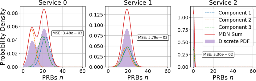
Figure 6: Validation of the proposed MDN model.

V-C Performance Analysis of the SNC-based Controller xApp

In a third set of experiments, we focus on a single decision period of the SNC-based Controller xApp. Specifically, we assume it computes $N_{\scriptscriptstyle m}^{\scriptscriptstyle min}$ for the three services described at the beginning of Section V. Under this scenario, we evaluate the convergence of the heuristics proposed in Algorithm 2, the computational complexity of such heuristics, and the accuracy of the obtained solution with respect to the optimal.

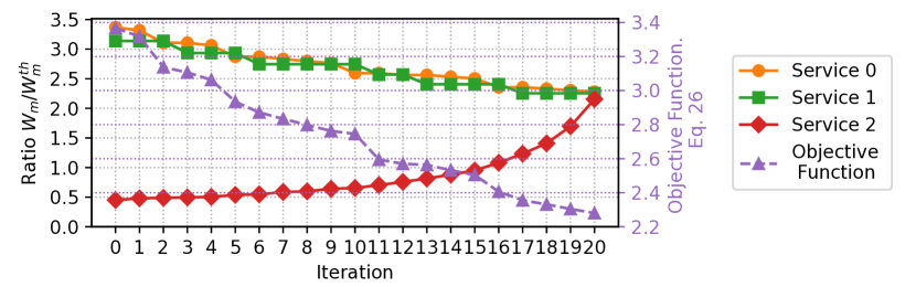
Figure 7: Convergence Analysis of Algorithm 2.

Fig. 7 shows the convergence of Algorithm 2. Specifically, it depicts the value of the objective function $g(\vec{W})$, i.e., purple curve, as well as the values of the ratios $W_{\scriptscriptstyle m}/W_{\scriptscriptstyle m}^{\scriptscriptstyle th}$ $\forall m\in\mathcal{M}$, i.e., orange, green and red curves, in each iteration. We observe how the proposed heuristics iteratively reduces $g(\vec{W})$ until reaching a suboptimal solution. In Fig.  8, we compare the solution obtained by the proposed heuristics with respect to the optimal one derived by brute force approach when considering $N_{\scriptscriptstyle cell}^{\scriptscriptstyle RB}\in[50,100]$ RBs. The relative error between the two curves is approximately $0.225\%$, indicating that the proposed solution yields only a 0.225% increase in the worst ratio $\nicefrac{{W_{\scriptscriptstyle m}}}{{W_{\scriptscriptstyle m}^{\scriptscriptstyle th}}}$ (see Eq. (24)) compared to the brute force approach. It is a reasonable deviation given the significant differences in computational complexity among the two approaches as Table I shows. Specifically, Table I summarizes the average execution time, the number of iterations, and the resulting ratio as a function of $N_{\scriptscriptstyle cell}^{\scriptscriptstyle RB}$. We observe the number of iterations monotonically increases with $N_{\scriptscriptstyle cell}^{\scriptscriptstyle RB}$ as the search space (i.e., combinations of RB allocation for each service) is greater, whereas the average execution time for a single iteration slightly decreases. Note that the tasks performed in a single iteration are the same for both approaches. The execution time per iteration decreases for larger $N_{\scriptscriptstyle cell}^{\scriptscriptstyle RB}$ values. This is due to the fact that the estimation of $W_{\scriptscriptstyle m}$ (i.e., when Algorithm 2 calls Algorithm 1 in step 5) is faster if more RBs are considered for each service. Specifically, we have experimentally observed that less iterations are needed by Algorithm 1 when $N_{\scriptscriptstyle cell}^{\scriptscriptstyle RB}$ increases, i.e., the value of $\theta_{\scriptscriptstyle z}$ (step 4) which minimizes Eq. (20) is greater.

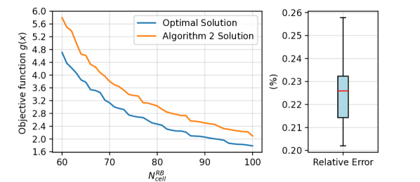
Figure 8: Performance Analysis of the SNC-based Controller.

TABLE I: Computational Complexity Comparison

$\mathbf{N_{cell}^{RB}}$	60	70	80	90	100
Brute Force (iterations)	1711	2346	3081	3916	4851
Algorithm 2 (iterations)	12	14	16	19	22
Ratio Algorithm 2 / Brute Force	142.58	167.57	192.56	206.10	220.5
Avg. Execution Time per iteration (ms)	184.62	179.09	176.39	173.76	171.85

V-D Performance Analysis of ORANUS framework

In the last experiment, we evaluated the performance of ORANUS against three reference solutions. The reference solution #1 consists of a single RT Controller using the EDF discipline. The reference solution #2 only considers the SNC-based Controller xApp. Note that this solution allocates dedicated RBs per service without sharing. The reference solution #3 considers the SNC-based Controller xApp and the RT Controller dApp. However, the RT Controller dApp does not use Algorithm 3.

To measure the performance of these solutions, we consider the Complementary Cumulative Distribution Function (CCDF) of the metric $(w-W_{\scriptscriptstyle m}^{\scriptscriptstyle th})/W_{\scriptscriptstyle m}^{\scriptscriptstyle th}$. Note the random variable $w$ represents the transmission delay of an arbitrary packet. Additionally, when this metric is equal to 0, the CCDF value represents the violation probability. In Fig. 9 we observe that the reference solution #2 provides the worst performance, i.e., a violation probability $11.46$ and $178.30$ times larger than ORANUS for services 1 and 2. Note that this probability is equal to 0 for scenario 3 when we consider ORANUS. These results are due to the fact the reference solution #2 only considers dedicated RBs. The remaining solutions consider sharing RBs among the services. Comparing them, the reference solution #1 usually provides a greater violation probability with respect to ORANUS. Although EDF ensures the packet with the earliest deadline are transmitted first, e.g., we observe for service 0 the CCDF is lower for reference solution #1 when $(w-W_{\scriptscriptstyle m}^{\scriptscriptstyle th})/W_{\scriptscriptstyle m}^{\scriptscriptstyle th}\leq 0$, it does not provide any guarantees in terms of violation probability. To consider such probability, the ORANUS framework establishes guaranteed RBs in a near-RT and allocates share free RBs among services using EDF in a RT scale. It improves the performance with respect to the remaining solutions. Specifically, ORANUS provides lower violation probabilities for service #1 and service #2. Finally, we observe the consideration of Algorithm 3 in ORANUS improves the obtained violation probability if we compare the results with respect to the ones obtained by the reference solution #3. The improvement is most significant when the metric $(w-W_{\scriptscriptstyle m}^{\scriptscriptstyle th})/W_{\scriptscriptstyle m}^{\scriptscriptstyle th}$ is higher. This is due to Algorithm 3 performing its actions when the waiting time of a packet in the transmission queue is closer to the delay budget. We can also observe the reference solution #3 has a similar behavior as ORANUS for service 2. The reason is the packet transmission delay never is above the delay budget for this service, as happens for services 0 and 1.

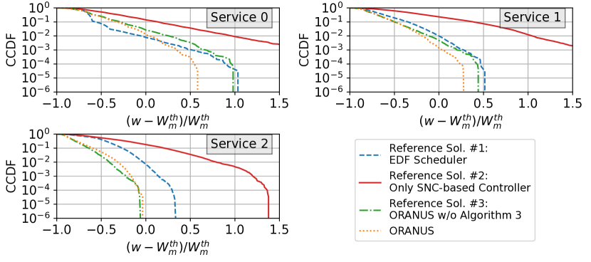
Figure 9: Complementary Cumulative Distribution Function (CCDF) for
$(w-W_{\scriptscriptstyle m}^{\scriptscriptstyle th})/W_{\scriptscriptstyle m}^{\scriptscriptstyle th}$. In ORANUS, we have set $\eta=0.75$ and $\tau=0.3$.

VI Related Work

Several works addressed the radio resource allocation problem in the presence of multiple uRLLC services. Concerning O-RAN based solutions, the authors of [25] propose a framework based on the actor-critic algorithm to minimize the probability of Internet of Things (IoT) devices’ age of information to exceed a predefined threshold. Despite its novelty, this work does not consider the transmission delay in the air interface. In [26], the authors propose an iterative algorithm to address the joint radio resource and power allocation problem, while the authors of [27] solve this problem by federated learning. In spite of their significance, their findings focus on the average delay as the key parameter. The authors of [28] analyze the performance of Deep Reinforcement Learnning (DRL) agents using a non-RT control loop that implements control actions in O-RAN. Despite its novelty, this solution omits details on the interactions of multi-time-scale control loops.

Focusing on non-RT and near-RT solutions, some works rely on queuing theory to model the packet transmission delay [29, 30, 31]. However, these models can only obtain average values when complex distributions are considered for the packet arrival rate and the channel capacity. Other works such as [7, 8, 9] use SNC to estimate a bound $W$ of type $\text{P}[w>W]<\varepsilon$, where $w$ is the packet transmission delay and $\varepsilon$ a target tolerance. However, they do not assume scenarios involving multiple uRLLC services nor their cross-interference. In [10], the authors propose a SNC-based controller for planning multiple uRLLC services. However, it considers dedicated radio resources for each service, which may result in resource wastage. Additionally, it is limited to traffic arrivals that follow a Poisson process with batches.

Considering RT solutions, works like [19, 32, 33] use schedulers based on EDF to assign priorities to packets based on their deadlines. EDF ensures the packets with the earliest deadline are transmitted first. However, EDF does not consider the probability the packet transmission delay exceeds a delay budget [34]. Other solutions such as [35, 36, 37] rely on ML models. Although they are effective in managing scenarios with intricate traffic patterns and channel conditions, their performance is primarily reliant on the similarity between the measured patterns and those used during training.

O-RAN specifications mention a RT control loop for optimizing tasks such as packet scheduling or interference recognition [38]. However, at the moment of writing this paper, such a control loop has not been defined. In the same row, the authors of [5] introduce the concept of dApps to implement fine-grained RT control tasks. Despite implementing a proof-of-concept, they omit to detail how multiple uRLLC services can be orchestrated in a RT scale, and how the near-RT control loop interacts with the dApps.

VII Conclusions

In this paper, we addressed the need of effective multi-time-scale control loops in O-RAN-based deployments for uRLLC services. Specifically, we proposed ORANUS, an O-RAN-compliant mathematical framework focused on the radio resource allocation problem at near-RT and RT scales. Focusing on the near-RT control loop, ORANUS relies on a novel SNC model to compute the amount of guaranteed RBs per service. Unlike traditional approaches as queueing theory, the SNC model allows ORANUS ensuring the probability the packet transmission delay exceeds a specific budget, i.e., the violation probability, is below a target tolerance. Another key novelty of ORANUS is the incorporation of a RT control loop which monitors the transmission queue of each service and dynamically adjusts the allocation of guaranteed RBs in response to traffic anomalies. We evaluated our proposal by a comprehensive simulation campaign, where ORANUS demonstrated substantial improvements, with an average violation probability $10\times$ lower, in comparison to reference solutions.

References

- [1] P. Popovski et al., “Wireless Access for Ultra-Reliable Low-Latency Communication: Principles and Building Blocks,” IEEE Netw., vol. 32, no. 2, pp. 16–23, 2018.
- [2] B. Tang, V. K. Shah, V. Marojevic, and J. H. Reed, “AI Testing Framework for Next-G O-RAN Networks: Requirements, Design, and Research Opportunities,” IEEE Wirel. Commun., vol. 30, no. 1, pp. 70–77, 2023.
- [3] A. S. Abdalla, P. S. Upadhyaya, V. K. Shah, and V. Marojevic, “Toward Next Generation Open Radio Access Networks: What O-RAN Can and Cannot Do!,” IEEE Netw., vol. 36, no. 6, pp. 206–213, 2022.
- [4] M. Polese, L. Bonati, S. D’Oro, S. Basagni, and T. Melodia, “Understanding O-RAN: Architecture, Interfaces, Algorithms, Security, and Research Challenges,” IEEE Commun. Surv. Tutor., pp. 1–1, 2023.
- [5] S. D’Oro, M. Polese, L. Bonati, H. Cheng, and T. Melodia, “dApps: Distributed Applications for Real-Time Inference and Control in O-RAN,” IEEE Commun. Mag., vol. 60, no. 11, pp. 52–58, 2022.
- [6] L. Zanzi, V. Sciancalepore, A. Garcia-Saavedra, H. D. Schotten, and X. Costa-Pérez, “LACO: A Latency-Driven Network Slicing Orchestration in Beyond-5G Networks,” IEEE Trans. Wirel. Commun., vol. 20, no. 1, pp. 667–682, 2021.
- [7] C. Xiao et al., “Downlink MIMO-NOMA for Ultra-Reliable Low-Latency Communications,” IEEE J. Sel. Areas Commun., vol. 37, no. 4, pp. 780–794, 2019.
- [8] S. Schiessl, M. Skoglund, and J. Gross, “NOMA in the Uplink: Delay Analysis With Imperfect CSI and Finite-Length Coding,” IEEE Trans. Wireless Commun., vol. 19, no. 6, pp. 3879–3893, 2020.
- [9] Á. A. Cardoso, M. V. G. Ferreira, and F. H. T. Vieira, “Delay bound estimation for multicarrier 5G systems considering lognormal beta traffic envelope and stochastic service curve,” Trans. Emerg. Telecommun. Technol., p. e4281, 2021.
- [10] O. Adamuz-Hinojosa, V. Sciancalepore, P. Ameigeiras, J. M. Lopez-Soler, and X. Costa-Pérez, “A Stochastic Network Calculus (SNC)-Based Model for Planning B5G uRLLC RAN Slices,” IEEE Trans. Wirel. Commun., vol. 22, no. 2, pp. 1250–1265, 2023.
- [11] O-RAN Working Group 3, “Near-Real-time RAN Intelligent Controller, Use Cases and Requirements 3.0,” Mar. 2023.
- [12] O-RAN Working Group 1, “Use Cases Analysis Report 10.0,” Mar. 2023.
- [13] M. Fidler and A. Rizk, “A Guide to the Stochastic Network Calculus,” IEEE Commun. Surveys Tuts., vol. 17, no. 1, pp. 92–105, 2015.
- [14] S. Ross, A First Course in Probability. Pearson, 2014.
- [15] C. M. Bishop, “Mixture Density Networks,” 1994.
- [16] B. Selim, O. Alhussein, S. Muhaidat, G. K. Karagiannidis, and J. Liang, “Modeling and Analysis of Wireless Channels via the Mixture of Gaussian Distribution,” IEEE Trans. Veh. Technol., vol. 65, no. 10, pp. 8309–8321, 2016.
- [17] K. Plataniotis and D. Hatzinakos, “Gaussian Mixtures and Their Applications to Signal Processing,” Advanced Signal Processing Handbook, CRC Press, pp. 89–124, 2017.
- [18] G. J. McLachlan, S. X. Lee, and S. I. Rathnayake, “Finite Mixture Models,” Annual Review of Statistics and Its Application, vol. 6, no. 1, pp. 355–378, 2019.
- [19] T. Guo and A. Suárez, “Enabling 5G RAN Slicing With EDF Slice Scheduling,” IEEE Trans. Veh. Technol., vol. 68, no. 3, pp. 2865–2877, 2019.
- [20] A. Elgabli, H. Khan, M. Krouka, and M. Bennis, “Reinforcement Learning Based Scheduling Algorithm for Optimizing Age of Information in Ultra Reliable Low Latency Networks,” in 2019 IEEE ISCC, pp. 1–6, 2019.
- [21] R. Falkenberg and C. Wietfeld, “FALCON: An Accurate Real-Time Monitor for Client-Based Mobile Network Data Analytics,” in 2019 IEEE GLOBECOM, pp. 1–7, 2019.
- [22] M. E. Haque, F. Tariq, M. R. A. Khandaker, K.-K. Wong, and Y. Zhang, “A Survey of Scheduling in 5G URLLC and Outlook for Emerging 6G Systems,” IEEE Access, vol. 11, pp. 34372–34396, 2023.
- [23] M. U. A. Siddiqui, H. Abumarshoud, L. Bariah, S. Muhaidat, M. A. Imran, and L. Mohjazi, “URLLC in Beyond 5G and 6G Networks: An Interference Management Perspective,” IEEE Access, vol. 11, pp. 54639–54663, 2023.
- [24] B. S. Khan, S. Jangsher, A. Ahmed, and A. Al-Dweik, “URLLC and eMBB in 5G Industrial IoT: A Survey,” IEEE Open J. Commun. Soc., vol. 3, pp. 1134–1163, 2022.
- [25] S. F. Abedin, A. Mahmood, N. H. Tran, Z. Han, and M. Gidlund, “Elastic O-RAN Slicing for Industrial Monitoring and Control: A Distributed Matching Game and Deep Reinforcement Learning Approach,” IEEE Trans. Veh. Technol., vol. 71, no. 10, pp. 10808–10822, 2022.
- [26] M. Karbalaee Motalleb, V. Shah-Mansouri, S. Parsaeefard, and O. L. Alcaraz López, “Resource Allocation in an Open RAN System Using Network Slicing,” IEEE Trans. Netw. Service Manag., vol. 20, no. 1, pp. 471–485, 2023.
- [27] F. Rezazadeh, L. Zanzi, F. Devoti, H. Chergui, X. Costa-Pérez, and C. Verikoukis, “On the Specialization of FDRL Agents for Scalable and Distributed 6G RAN Slicing Orchestration,” IEEE Trans. Veh. Technol., vol. 72, no. 3, pp. 3473–3487, 2023.
- [28] M. Polese, L. Bonati, S. D’Oro, S. Basagni, and T. Melodia, “ColO-RAN: Developing Machine Learning-based xApps for Open RAN Closed-loop Control on Programmable Experimental Platforms,” IEEE Trans. Mob. Comput., pp. 1–14, 2022.
- [29] W. Zhang, M. Derakhshani, G. Zheng, C. S. Chen, and S. Lambotharan, “Bayesian Optimization of Queuing-Based Multichannel URLLC Scheduling,” IEEE Trans. Wirel. Commun., vol. 22, no. 3, pp. 1763–1778, 2023.
- [30] B. Shi, F.-C. Zheng, C. She, J. Luo, and A. G. Burr, “Risk-Resistant Resource Allocation for eMBB and URLLC Coexistence Under M/G/1 Queueing Model,” IEEE Trans. Veh. Technol., vol. 71, no. 6, pp. 6279–6290, 2022.
- [31] P. Yang, X. Xi, T. Q. S. Quek, J. Chen, X. Cao, and D. Wu, “RAN Slicing for Massive IoT and Bursty URLLC Service Multiplexing: Analysis and Optimization,” IEEE Internet Things J., vol. 8, no. 18, pp. 14258–14275, 2021.
- [32] I. Hadar, L.-O. Raviv, and A. Leshem, “Scheduling For 5G Cellular Networks With Priority And Deadline Constraints,” in IEEE ICSEE, pp. 1–5, 2018.
- [33] L.-O. Raviv and A. Leshem, “Joint Scheduling and Resource Allocation for Packets With Deadlines and Priorities,” IEEE Commun. Lett., vol. 27, no. 1, pp. 248–252, 2023.
- [34] F. Capozzi, G. Piro, L. Grieco, G. Boggia, and P. Camarda, “Downlink Packet Scheduling in LTE Cellular Networks: Key Design Issues and a Survey,” IEEE Commun. Surv. Tutor., vol. 15, no. 2, pp. 678–700, 2013.
- [35] J. Zhang, X. Xu, K. Zhang, B. Zhang, X. Tao, and P. Zhang, “Machine Learning Based Flexible Transmission Time Interval Scheduling for eMBB and uRLLC Coexistence Scenario,” IEEE Access, vol. 7, pp. 65811–65820, 2019.
- [36] A. A. Esswie, K. I. Pedersen, and P. E. Mogensen, “Online Radio Pattern Optimization Based on Dual Reinforcement-Learning Approach for 5G URLLC Networks,” IEEE Access, vol. 8, pp. 132922–132936, 2020.
- [37] M. Alsenwi, N. H. Tran, M. Bennis, S. R. Pandey, A. K. Bairagi, and C. S. Hong, “Intelligent Resource Slicing for eMBB and URLLC Coexistence in 5G and Beyond: A Deep Reinforcement Learning Based Approach,” IEEE Trans. Wirel. Commun., vol. 20, no. 7, pp. 4585–4600, 2021.
- [38] O-RAN Working Group 2, “O-RAN AI/ML workflow description and requirements 1.03,” July 2021.