In-vacuo dispersion from $\kappa$-anti-de Sitter algebra

Abstract

Based on deformed translations in $\kappa$-anti-de Sitter algebra, we derive a delay in the time of detection between a soft and a hard photon which are simultaneously emitted at a distant event, at first order in the quantum gravity parameter. In the basis analyzed, the trajectories are undeformed and the effect depends exclusively on the symmetry properties of the quantum algebra. The time delay depends linearly on the energy of the hard particle and has a sinusoidal dependence on the redshift of the source.

I Introduction

The quantization of gravity is one of the most challenging problems of science, and that has been examined by some generations of physicists and mathematicians in the past decades. Despite some success in constructing theories that capture different aspects of the expected nature of a quantum spacetime or of the quantum nature of the gravitational interaction, like canonical quantum gravity Kiefer:2004xyv , string theoryPolchinski:1998rq ; Polchinski:1998rr , loop quantum gravity Ashtekar:2021kfp , causal dynamical triangulation Loll:2019rdj and asymptotic safety Eichhorn:2018yfc , no experimental verification that validates any of these approaches has been found yet.

A common result in many of these approaches is that in the asymptotic limit that approaches the low gravity regime or low energy scale, the physical observables are given by perturbations of equations of special/general relativity or quantum mechanics Amelino-Camelia:2008aez . Furthermore, that such corrections are suppressed by a scale that is usually proportional to planckian units. As this regime is so far reaching when we consider typical energies of elementary particles in accelerators, the quantization of the gravitational interaction has been assumed as a purely mathematical and philosophical curiosity for many years. However, with the development of the area of astroparticle physics, this picture has changed, since we are not only able to detect particles with higher energies, but also the length in which these particles propagate are much longer than in accelerators: a property that is responsible for amplifying the tiny planckian corrections Amelino-Camelia:2008aez ; Addazi:2021xuf . These new inputs, along with improvement in detection precision by observatories, have led to the dawn of the area of quantum gravity phenomenology by the end of the 20th century, whose capability of constraining quantum gravity-inspired corrections with Planck scale sensitivity has been achieved in the past few years fermigbmlat:2009nfe and presents many appealing windows to be explored in the next years AlvesBatista:2023wqm .

The most explored of these avenues is the phenomenon called in-vacuo dispersion Addazi:2021xuf , which is the dependence of massless particles’ speed with their energy, and is a prediction of several approaches to quantum gravity Amelino-Camelia:2008aez ; Gambini:1998it ; Amelino-Camelia:2016gfx and other forms of Lorentz Invariance Violation (LIV) scenarios, like extensions of the standard model theories Kostelecky:2003fs . The standard assumption in the derivation of in-vacuo dispersion bounds is the Jacob-Piran formula Jacob:2008bw ; Ellis:2002in , that gives the dependence on particles energies and propagation distance dependence for the time delay from the arrival of massless particles when they are simultaneously emitted in a given source.

As was shown in Amelino-Camelia:2012vzf ; Rosati:2015pga , the main assumptions of the Jacob-Piran formula Jacob:2008bw is the minimal coupling between the particles’ momentum and local violation of Poincaré symmetry (rotations, boosts and translations). The relaxation of these hypotheses has been explored in some recent works on curvature-triggered effects Amelino-Camelia:2020bvx ; Amelino-Camelia:2022pja ; Amelino-Camelia:2023srg and other ansatze for defining such delay Pfeifer:2018pty . For instance, if instead of violation, one incorporates in the derivation a deformation of local Poincaré symmetry that preserves the quantum gravity departures of relativistic equations, one actually finds corrections to Jacob-Piran formula, that could actually better fit the data from astrophysical events, as has been shown in the preliminary work Bolmont:2022yad . This deformation has been initially shown for the special case of assuming that the spacetime has a Planck-scale-deformed de Sitter structure, where a deformation of the de Sitter algebra has been the background of the derivation, which besides presenting deformed worldlines (that coincide with Jacob-Piran’s ansatz), presents also deformed translation transformations, which governs the communication between the distant frames given by the emission and detection events. We should stress that calculating such kind of effect in a Deformed Special Relativity (DSR) scenario Amelino-Camelia:2000stu using modified translations (following the lessons of the principle of relative locality Amelino-Camelia:2011lvm ) is of utmost importance to avoid non-local pathologies pointed out by different authors Schutzhold:2003yp ; Hossenfelder:2010tm , whose solutions were discussed in Amelino-Camelia:2011uwb .

Although the de Sitter case has been extensively explored in the literature, deformations of the anti-de Sitter (AdS) algebra from the point of view of time delays has been neglected, despite the dedicated theoretical work that has been devoted to rigorously formulating the features of a quantum deformation of anti-de Sitter algebra Ballesteros:2016bml , in which not only the full set of isometries are explored, but also the co-product structure in AdS space for multiparticle systems and its carrollian and galilean limits Ballesteros:2021dob .

In this paper, we fill this gap and derive a time delay formula, that depends on the energy of a hard (high energy) massless particle simultaneously emitted with a soft one (low energy) in a given spacetime event, following the recipe discussed in Amelino-Camelia:2012vzf , but applied to the quantum deformation of the anti-de Sitter algebra described in Ballesteros:2016bml , at first order in the quantum gravity scale.

The paper is organized as follows. In section II, we revise the classical mechanics of anti-de Sitter spacetime by the derivation of the conserved charges from the Killing equations in cosmological coordinates and the associated Casimir that is the mass shell. In section III, we find the dependence of the symmetry generators and Casimir charge of the $\kappa$-AdS algebra in terms of the classical ones. In section IV, we express the translation generators in conformal coordinates, which are easier to handle computationally. In section V, we use the deformed translations to derive the time delay of the $\kappa$-AdS spacetime from the basis rigorously explored in Ballesteros:2016bml . We draw our final remarks in section VI. We are assuming natural units, such that $\hbar=c=1$.

II Classical Mechanics and Symmetries in Anti-de Sitter Space

Before we proceed to the derivation of the deformed kinematics of particles in anti-de Sitter geometry, we revisit its simpler, classical counterpart. In this section, we are mostly relying on purely algebraic tools to derive our results, however our starting point is the derivation of symmetry generators in AdS space. As is usually the case of similar analyses, we shall rely on the $1+1$ dimensional example. The generators of symmetries are conserved charges, therefore they should be found from the Killing vectors in a given spacetime. For AdS space, we consider the metric given by the following line element of FLRW type Magueijo:2009ff

$$ds^{2}=dt^{2}-\cos^{2}(\lambda t)dx^{2}=g_{\mu\nu}dx^{\mu}dx^{\nu}\,,$$ (1)

where the parameter $\lambda$ is related to the anti-de Sitter curvature as $\Lambda=-\lambda^{2}$. We solve the Killing equation $\nabla_{\mu}K_{\nu}+\nabla_{\mu}K_{\mu}=0$, for the Killing vector $K_{\mu}$, which in $1+1$ dimensions presents only three solutions, which are responsible for describing time translation $K^{\mu}_{(0)}$, space translation $K^{\mu}_{(1)}$ and spacetime boost $K^{\mu}_{(2)}$. The energy $E_{0}$, momentum $P_{0}$ and boost generator $N$ are conserved charges, given by

$$E_{\circ} = K^{\mu}_{(0)}p_{\mu}=\cosh{(\lambda x)}p_{0}+\sinh{(\lambda x)}\tan{(\lambda t)}p_{1}\,,$$ (2)

$$P_{\circ} = K^{\mu}_{(1)}p_{\mu}=p_{1}\,,$$ (3)

$$N_{\circ} = K^{\mu}_{(2)}p_{\mu}=\frac{\sinh{(\lambda x)}}{\lambda}p_{0}+\cosh{(\lambda x)}\frac{\tan{(\lambda t)}}{\lambda}p_{1}\,,$$ (4)

where we use the subscript “$\circ$” in these expressions to stress that we are considering the classical anti-de Sitter generators.

Considering that the generalized coordinates $(t,x,p_{0},p_{1})$ are canonical, i.e., that

$$\{t,p_{0}\}=1=\{x,p_{1}\}\,,$$ (5)

and zero otherwise, we verify that the above charges define a Lie algebra as follows

$$\{E_{\circ},P_{\circ}\} = \lambda^{2}N_{\circ}=-\Lambda N_{\circ}\,,$$ (6)

$$\{N_{\circ},P_{\circ}\} = E_{\circ}\,,$$ (7)

$$\{N_{\circ},E_{\circ}\} = P_{\circ}\,,$$ (8)

where the Poisson brackets of two phase space quantities $F$ and $G$ are

$$\{F,G\}=\frac{\partial F}{\partial x^{\mu}}\frac{\partial G}{\partial p_{\mu}}-\frac{\partial F}{\partial p_{\mu}}\frac{\partial G}{\partial x^{\mu}}=\frac{\partial F}{\partial\eta}\frac{\partial G}{\partial p_{0}}+\frac{\partial F}{\partial x}\frac{\partial G}{\partial p_{1}}-\frac{\partial F}{\partial p_{0}}\frac{\partial G}{\partial t}-\frac{\partial F}{\partial p_{1}}\frac{\partial G}{\partial t}$$ (9)

This is the known algebra of anti-de Sitter generators in $1+1$-dimensions, $\text{AdS}_{\Lambda}$ Ballesteros:2016bml . The Casimir operator related to this algebra is given by Eq.(2.2) of Ballesteros:2016bml and in cosmological coordinates read

$$C_{\circ}=E_{\circ}^{2}-P_{\circ}^{2}-\lambda^{2}N_{\circ}^{2}=p_{0}^{2}-\sec^{2}{(\lambda t)}p_{1}^{2}\,,$$ (10)

which is simply the norm $g^{\mu\nu}p_{\mu}p_{\nu}$ using the metric defined by the line element (1).

II.1 Classical Trajectories

The trajectories can be easily found using the Casimir (10) as the generator of the parametrization evolution (here “dot” means derivative with respect to an affine parameter)

$$\dot{t} = \{t,C_{\circ}\}=2p_{0}\,,$$ (11)

$$\dot{x} = \{x,C_{\circ}\}=-2p_{1}\sec^{2}{(\lambda t)}\,,$$ (12)

$$\dot{p_{0}} = \{p_{0},C_{\circ}\}=2\lambda p_{1}^{2}\sec^{2}{(\lambda t)}\tan^{2}{(\lambda t)}\,,$$ (13)

$$\dot{p_{1}} = \{p_{1},C_{\circ}\}=0\,.$$ (14)

To derive an equation of the kind $x(t)$, we need to express the equation $dx/dt=\dot{x}/\dot{t}$ using Eqs.(11) and (12). This gives an equation that depends on $t$ and $p_{0}$. However, we can also express $p_{0}$ as a function of $t$ for the trajectories of particles with mass $m$, i.e., those for which $C_{\circ}=m^{2}$ in (10). This gives

$$\frac{dx}{dt}=-\frac{p_{1}\sec^{2}{(\lambda t)}}{\sqrt{m^{2}+\sec^{2}{(\lambda t)}p_{1}^{2}}}\,.$$ (15)

This equation can be solved analytically for any mass $m$. For the massless case $m\rightarrow 0$ and out-going particles $p_{1}<0$, we find

$$x(t)=x_{0}+\frac{\operatorname{arctanh}{[\sin(\lambda t)]}}{\lambda}\,.$$ (16)

This is the affine null geodesic of AdS spacetime.

II.2 Classical Translations

Using the canonical brackets (5), we can construct the infinitesimal translations in time and space, and the boost by the action of the generators $E_{\circ}$ (2), $P_{\circ}$ (3) and $N_{\circ}$ (4)

$$\{t,E_{\circ}\} = \cosh{(\lambda x)}\,,$$ (17)

$$\{t,P_{\circ}\} = 0\,,$$ (18)

$$\{t,N_{\circ}\} = \frac{\sinh{(\lambda x)}}{\lambda}\,,$$ (19)

$$\{x,E_{\circ}\} = \sinh{(\lambda x)}\tan{(\lambda t)}\,,$$ (20)

$$\{x,P_{\circ}\} = 1\,,$$ (21)

$$\{x,N_{\circ}\} = \cosh{(\lambda x)}\frac{\tan{(\lambda t)}}{\lambda}\,.$$ (22)

Similar rules could be found for momenta, but since we will not use them in this paper, we shall not dwell with them here. In any case, endowed with these tools, we have finite transformations $T_{G;a}$ generated by a charge $G$, parametrized by the quantity $a$, acting of a phase space quantity $X=X(t,x,p_{0},p_{1})$ as (called an exponentiation)

$$T_{G;a}\triangleright X=e^{-aG}\triangleright X=\sum_{n=0}^{\infty}\frac{(-a)^{n}}{n!}\{X,G\}_{n}\,,$$ (23)

where $\{X,G\}$ is recursively defined as

$$\{X,G\}_{0} = X\,,$$ (24)

$$\{X,G\}_{n} = \{\{X,G\}_{n-1},G\}\,.$$ (25)

This allows us to translate individual events and trajectories in AdS spacetime, for example. In the following, we shall consider the deformed case and derive similar analytical mechanics results using a deformed version of the AdS algebra.

III Quantum Deformation of Anti-de Sitter Algebra

In this section, we rely mainly on results reported in Ballesteros:2016bml , that describes the $\kappa$-AdS algebra, as a deformation of the anti-de Sitter algebra by the presence of a parameter with dimensions of energy $\kappa^{-1}\doteq\ell$, which supposedly is proportional to the invarian quantum gravity energy scale. In $1+1$-dimensions, this algebra presents the following Poisson brackets

$$\{N,E\} = P\,,$$ (26)

$$\{E,P\} = \lambda^{2}N\,,$$ (27)

$$\{N,P\} = \frac{1}{2\ell}(1-e^{-2\ell E})-\frac{\ell}{2}P^{2}-\frac{\ell\lambda^{2}}{2}N^{2}\approx E-\ell\left[E^{2}-\frac{P^{2}}{2}-\frac{\lambda^{2}}{2}N^{2}\right]\,,$$ (28)

where we are considering only first order terms in $\ell$. Besides that, the deformed Casimir is

$$C=\frac{1}{2\ell^{2}}(\cosh{(\ell E)}-1)-e^{\ell E}(P^{2}+\lambda^{2}N^{2})\approx E^{2}-P^{2}-\lambda^{2}N^{2}+\ell\left(EP^{2}-\lambda^{2}EN^{2}\right)\,.$$ (29)

As can be seen, we can treat this formalism as $\kappa$-deformation of the AdS algebra (which is recovered when $\ell=\kappa^{-1}\rightarrow 0$), or as a $\Lambda$-deformation of the $\kappa$-Poincaré algebra Ballesteros:2021dob (which is recovered when $\lambda=\sqrt{-\Lambda}\rightarrow 0$).

Considering the former viewpoint, we can also treat the generators $(E,P,N)$ as $\kappa$-deformations of the AdS ones considered in the previous section $(E_{\circ},P_{\circ},N_{\circ})$. At this point, we need to make some simplificatons and bear our intuition on similar approaches previously studied in the literature. Due to the isotropy of this approach, we shall assume that the space translation generator is not modified by the $\kappa$-corrections and is given by the anti-de Sitter one considered in the previous section, i.e., $P=P_{\circ}$. We should stress that this same property applies to the $\kappa$-de Sitter algebra considered by other authors, as can be seen in Eq.(19) of Amelino-Camelia:2012vzf . As we will see, this is a valid representation of this algebra. The rest of the analysis is done according to the following ansatz

$$N = N_{\circ}+\ell f(E_{\circ},P_{\circ},N_{\circ})\,,$$ (30)

$$E = E_{\circ}+\ell(\alpha E_{\circ}^{2}+\beta E_{\circ}P_{\circ}+\gamma P_{\circ}^{2}+\delta\lambda E_{\circ}N_{\circ}+\epsilon\lambda P_{\circ}N_{\circ}+\phi\lambda^{2}N_{\circ}^{2})\,,$$ (31)

$$P = P_{\circ}\,,$$ (32)

where $g$ is a function of the undeformed charges, and $(\alpha,\beta,\gamma,\delta,\epsilon,\phi)$ are dimensionless parameters that shall be fixed a posteriori. We can find the form of the function $f$ by substituting Eqs.(30)-(32) in the relation (27). Using the underformed brackets (6), (7), (8) in this expression, we find that the function $g$ must have the following form

$$f=2\alpha N_{\circ}E_{\circ}+\beta N_{\circ}P_{\circ}+\frac{\delta}{\lambda}(\lambda^{2}N_{\circ}^{2}+E_{\circ}^{2})+\frac{\epsilon}{\lambda}P_{\circ}E_{\circ}+2\phi N_{\circ}E_{\circ}\,.$$ (33)

Now, we use this form of $f$ into $N$ (40) and consider the bracket $\{N,E\}$ in (26) (where we also use the brackets involving the underformed generators (6), (7), (8)). Isolating the factors that multiply the product of independent charges $E_{\circ}^{2},\,N_{\circ}^{2},\,P_{\circ}^{2},\,N_{\circ}P_{\circ},\,N_{\circ}E_{\circ},\,E_{\circ}P_{\circ}$, we find the following set of conditions

$$\beta = \delta=0\,,$$ (34)

$$\phi = -2\alpha-\gamma\,,$$ (35)

and $\epsilon$ remains an arbitrary parameter. We consider this simplification in the definition of $N$ and $E$, given by (30) and (31), to analyze the bracket $\{N,P\}$. Therefore, using (6), (7), (8) into (28), we isolate the factors that multiply the products of underformed charges to further constrain the remaining parameters as

$$\alpha = \beta=\delta=0\,,$$ (36)

$$\gamma = \frac{1}{2}\Rightarrow\phi=-\frac{1}{2}\,,$$ (37)

$$\epsilon = \text{arbitrary}\,.$$ (38)

This leads us to the following expression of the deformed charges in terms of the undeformed ones

$$E = E_{\circ}+\ell\left(\frac{P_{\circ}^{2}}{2}-\frac{\lambda^{2}}{2}N_{\circ}^{2}+\epsilon\lambda P_{\circ}N_{\circ}\right)\,,$$ (39)

$$N = N_{\circ}+\ell\left(\frac{\epsilon}{\lambda}P_{\circ}E_{\circ}-N_{\circ}E_{\circ}\right)\,,$$ (40)

$$P = P_{\circ}\,.$$ (41)

To check the consistency of this result, it is sufficient to check that Eqs.(26), (27), (28) are satisfied (using the undeformed expressions (6), (7), (8)). We can express these charges in cosmological coordinates $(t,x,p_{0},p_{1})$ by using Eqs.(2), (3), (4). It is interesting to notice the presence of an arbitrary parameter $\epsilon$, that as we will see, will play a non-trivial role in the behavior of the time delay. Also, we would like to remark that in other approaches that analyze the de Sitter case, for example in Amelino-Camelia:2012vzf , arbitrary parameters are also present.

Endowed with these expressions, we can calculate the deformed Casimir operator in terms of the undeformed charges as well. Substituting Eqs.(39), (40), (41) into the Casimir charge (29), we find

$$C=E^{2}-P^{2}-\lambda^{2}N^{2}+\ell\left(EP^{2}-\lambda^{2}EN^{2}\right)+{\cal O}(\ell^{2})=E_{\circ}^{2}-P_{\circ}^{2}-\lambda^{2}N_{\circ}^{2}+{\cal O}(\ell^{2})=C_{\circ}+{\cal O}(\ell^{2})\,.$$ (42)

Surprisingly, we do not find first order corrections on the Casimir operator when we express it in terms of the undeformed charges (and this is a coordinate independent statement). For this reason, we would find, for example, that the dispersion relation of particles in this scenario is given by the undeformed expression (10). This implies that the trajectory of a massless particle is unmodified and is given by (16). A similar issue on the difference between the symmetry generators and the energy and momentum of photons is also discussed in footnote 4 of Carmona:2022pro .

As we shall see, despite the absence of a deformed trajectory, we will be able to find a time delay at first order in $\ell$ due to the presence of deformed translations generated by $E$ and $P$. In fact, we can express the infinitesimal transformation generated by these charges by using their dependence with the undeformed ones and the actions already calculated in (17)-(22).

IV Translations in Conformal Coordinates

Some lessons considered in previous investigations by other authors on the de Sitter case can be applied to ours, as for example, the fact that the use conformally flat coordinates simplifies a lot the computations needed to find finite translations. The AdS line element can be cast in conformally flat coordinates by the definition of a conformal time $\eta$

$$d\eta=\sec{(\lambda t)}dt\Rightarrow\eta=\frac{\operatorname{arctanh}{[\sin(\lambda t)]}}{\lambda}\,,$$ (43)

in which the line element (1) assumes the form $ds^{2}=\operatorname{sech}^{2}{(\lambda\eta)}(d\eta^{2}-dx^{2})$. As the undeformed charges (2)-(4) are scalars from the point of view of coordinate transformations, then in order to express them in coordinates $(\eta,x)$, we must simply perform the transformation (43) on the time coordinate and correspondingly express the momenta $p_{\mu}$ in the novel coordinates (which gives the same result of transforming $K^{\mu}$ to new coordinates as calculating $K^{\prime}{}^{\mu}p^{\prime}_{\mu}$). Let us dub the energy and momentum in these new coordinates as $(\Omega,\Pi)$, respectively. One can easily verify that the following relation is valid

$$p_{0} = \frac{d\eta}{dt}\Omega=\cosh{(\lambda\eta)}\Omega\,,$$ (44)

$$p_{1} = \Pi\,.$$ (45)

For this reason, the undeformed conserved charges read

$$E_{\circ} = \cosh{(\lambda\eta)}\cosh{(\lambda x)}\Omega+\sinh{(\lambda\eta)}\sinh{(\lambda x)}\Pi\,,$$ (46)

$$P_{\circ} = \Pi\,,$$ (47)

$$N_{\circ} = \frac{\cosh{(\lambda\eta)}\sinh{(\lambda x)}\Omega}{\lambda}+\frac{\sinh{(\lambda\eta)}\cosh{(\lambda x)}\Pi}{\lambda}\,.$$ (48)

In fact, using this representation of the charges, the Casimir (29) takes the form

$$C_{\circ}=\cosh^{2}{(\lambda\eta)}(\Omega^{2}-\Pi^{2})\,,$$ (49)

as expected. Besides that, as the analysis done in the previous section regarding the $\kappa$-AdS algebra was performed in a coordinate-invariant way, the same results discussed previously are preserved in these conformally flat coordinates. In these coordinates, the massless trajectories are simply straight lines.

V Time delay in $\kappa$-Anti-de Sitter Space

In order to connect distant events by the emission and detection of light rays, we need to consider these events as if they were local to relatively distant observers, for instance Alice and Bob. We shall consider a thought experiment in which massless particles with different energies are emitted in a single event that coincides with the origin of the coordinate system associated with the observer Alice and are detected at the $x$-axis of the observer Bob with a delay in time coordinates.

In order to find this delay, we need to translate the geodesics from Alice’s coordinates to Bob’s coordinates, which include translating the inicial conditions from Alice’s coodinate system to Bob’s. A difference in the location of the emission event will appear in Bob’s coordinates due to deformed translations and this is intimately related the principle of relative locality, in which the location, in spacetime, of a distant event is described by a distant observer as if nonlocal. This is just an apparent nonlocality, since for an observer close enough to the emission event (Alice), it takes place objectively at a single spacetime event.

For this reason, we will need to translate the origin of Alice’s coordinate system to express it in terms of Bob’s coordinates. This is done by acting with a finite translation as defined in (23) as

Bob $$= e^{-a_{x}P}\triangleright e^{-a_{\eta}E}\triangleright\text{Alice}\Rightarrow$$ (50)

$$(\eta_{0}^{B},x_{0}^{B}) = e^{-a_{x}P}\triangleright e^{-a_{\eta}E}\triangleright(0,0)\,.$$ (51)

In this representation, the coordinates $(\eta,x,\Omega,\Pi)$ are canonical since the charges are scalar quantities and the Poisson brackets are invariant under coordinate transformations. From the definition of $E$ and $P$ in (39), (41), along with the undeformed charges in conformally flat coordinates (46), (47), (48), we notice that space translations generated by $P$ are undeformed, do not affect the time coordinate and simply shifts the spatial one, while time translations presents an energy-dependence. Performing the series of operations defined in (23), we exponentiate the translations, and after a tedious computation, we find the following result when applied to the point $(0,0)$ (verified until 6th order perturbation in $a_{\eta}$)

$$\eta_{0}^{B} = \eta_{0}^{B}|_{\ell=0}+{\cal O}(\ell^{2})\,,$$ (52)

$$x_{0}^{B} = -a_{x}-\frac{\ell\Pi}{\lambda}\sin{(\lambda a_{\eta})}[1-\epsilon\tan{(\lambda a_{\eta})}]+{\cal O}(\ell^{2})\,,$$ (53)

where $\eta_{0}^{B}|_{\ell=0}$ is the undeformed translated origin, in Bob’s coordinates, in classical anti-de Sitter space, that we shall not dwell with in this paper. This is the central set of equations of this paper, and from it the time delay is calculated straightforwardly.

In fact, in this gedankenexperiment, two massless particles (that we simply call photons) are emitted simultaneously from Alice’s origin: a soft photon with momentum $\Pi_{s}$, whose kinematics is unaffected by $\kappa$-corrections, and a hard photon with momentum $\Pi_{h}$, whose kinematics presents Planck-scale corrections. As we calculated that both particles present the same dispersion relation at first order in $\ell$ (in terms of classical generators), their trajectories are the same concerning the soft and hard photons. Since Alice and Bob’s origin are connected by the soft photon trajectory, we set $\eta_{0}^{B}|_{\ell=0}=-a_{x}$. Below, we express the photons trajectories in the conformally flat patch using Alice and Bob’s coordinates, where we use the superscript “$A$” and “$B$” to represent them

$$x^{A,B}_{s} = x^{A,B}_{0;s}+\eta^{A,B}_{s}-\eta^{A,B}_{0;s}\,,$$ (54)

$$x^{A,B}_{h} = x^{A,B}_{0;h}+\eta^{A,B}_{h}-\eta^{A,B}_{0;h}+{\cal O}(\ell^{2})\,.$$ (55)

The time delay is a difference in the time coordinates of both particles when they reach the same location in Bob’s coordinates, i.e., when $x^{B}_{s}=x^{B}_{h}$ in (54), (55). We can assume, without loss of generality, that the soft particle reaches the origin of Bob’s coordinate system, i.e., $\eta^{B}_{s}=0$ in (54). Using these conditions, along with (52), (53) we subtract Eqs.(54) and (55) to find

$$\Delta\eta^{B}=\eta^{B}_{h}-\eta^{B}_{s}=\eta^{B}_{h}=x^{B}_{0;s}-x^{B}_{0;h}=\frac{\ell}{\lambda}\Pi_{h}\sin{(\lambda a_{\eta})}[1-\epsilon\tan{(\lambda a_{\eta})}]\,.$$ (56)

From this expression, we identify a problem with the freedom to consider the parameter $\epsilon$, as it introduces a discontinuous behavior in the time delay whenever $\epsilon\neq 0$. The reason is that the tangent function diverges at $\pi/2$, (therefore at $\lambda a_{\eta}=\pi/2)$). As such discontinuity brings a nonphysical behavior (since there’s nothing special such value of $a_{\eta}$), we set $\epsilon=0$. We depict the relative locality effect in conformal coordinates in Fig.1. As can be seen, the emission event (local in Alice’s coordinate) appears nonlocal in Bob’s coordinates. This is the origin of the time delay effect even with undeformed trajectories.

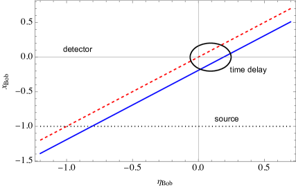
Figure 1: $\kappa$-AdS trajectories of photons in Bob’s conformal coordinates. The red/dashed line describes the soft photon emitted at $x^{B}_{0;s}=-a_{x}=-a_{\eta}=-5$ in Bob’s coordinates. Although the emission occurs at the same spacetime location in Alice’s coordinates $(t^{A}_{0;s},x^{A}_{0;s})=(t^{A}_{0;h},x^{A}_{0;h})=(0,0)$, it seems displaced in Bob’s coordinates due to relative locality. The blue/solid line describes the trajectory of the hard photon for $|p|=1$, $\ell=0.2$ and $\lambda=1$.

Due to its oscillatory behavior, the time delay can be positive or negative, depending on the distance between the detector and the source. In Fig.2, we describe the conformal time delay as function of $a_{\eta}$, where we located the detector in the origin of Bob’s coordinate system. This oscillatory behavior does not obey exactly the intuition of the time delays literature, in which the effect should grow with the distance between the source and the detector, but the point is that the trajectories in this case are classical, so we depend exclusively on the symmetry properties of the anti-de Sitter space, which as we know presents an exotic behavior, like the presence of closed timelike curves and that some geodesics usually converge, expand and reconverge, so such oscillatory behavior should not be a complete surprise. Such general properties are discussed in section 5.2 of Hawking:1973uf .

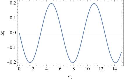
Figure 2: Conformal time delay as a function of the translation parameter $a_{\eta}$ for $\lambda=1=|p|$, $\ell=0.2$. We can have positive or negative delays due to the oscillatory behavior of $\kappa$-AdS symmetries.

In order to compare this result with the Jacob-Piran ansatz, we express it in terms of the redshift function and the cosmological time. By Eq.(43), we have that the relation between the redshift $z$, cosmological scale factor $a(t)$ and conformal time is the following

$$\frac{1}{1+z} = a(t)=\cos{(\lambda t)}=\operatorname{sech}{(\lambda\eta)}\Rightarrow$$ (57)

$$\eta(z) = \frac{1}{\lambda}\operatorname{arcsech}{\left(\frac{1}{1+z}\right)}\,.$$ (58)

For this reason, the translation parameter is related to the redshift as $a_{\eta}=\lambda^{-1}\operatorname{arccosh}{(1+z)}$.

Considering that $t=\lambda^{-1}\arcsin{(\tanh{(\lambda\eta)})}$ and that, as we discussed below Eq.(15), we have $\Pi=p_{1}\doteq p<0$, we express the time delay in cosmological coordinates as (we see that $\Delta\eta=\Delta t+{\cal O}(\ell^{2})$)

(59)

This is the main result of our paper. It is the description of a time delay from the $\kappa$-anti-de Sitter algebra. It does not present deformed trajectories, yet due to the presence of deformed translations, a time delay is presented.

For small redshifts, this expression assumes the form

$$\Delta t|_{z\ll 1}\approx-\frac{\ell|p|}{\lambda}\left(\sqrt{2z}-\frac{5z^{3/2}}{6\sqrt{2}}\right)\,.$$ (60)

The same kind of powers in redshift would appear had one considered the Jacob-Piran formula Jacob:2008bw for an anti-de Sitter space with scale factor $a(t)=\cos{(t)}$ and a modified dispersion relation of the kind $p_{0}^{2}-\sec^{2}{(\lambda t)}p^{2}+\ell\sec^{3}{(\lambda t)}|p|^{3}=0$ (where $H(t)=a(t)^{-1}da(t)/dt$)

$$\Delta t_{JP,z\ll 1}=\ell|p|\int_{0}^{z}\frac{1+\bar{z}}{H(\bar{z})}d\bar{z}\approx-\frac{\ell|p|}{\lambda}\left(\sqrt{2z}-\frac{z^{3/2}}{2\sqrt{2}}\right)\,.$$ (61)

In Fig.3, we depict the $\kappa$-AdS time delay of Eq.(59) in blue, and the Jacob-Piran time delay of Eq.(61) in orange. We see that both formulas agree for small delays, but then, the oscillatory behavior of the $\kappa$-AdS time delay generated by the translations of AdS space pulls back the time delay. Usually, one expects that the relative locality effects should grow with the distance between the source and the detector, but we are showing that this is not always the case. The delay that we presented is bounded despite of the relative distance between the events and can also be null. A similar behavior can be found in more recent analyses carried out in Amelino-Camelia:2023srg , where such richer class of delays is presented.

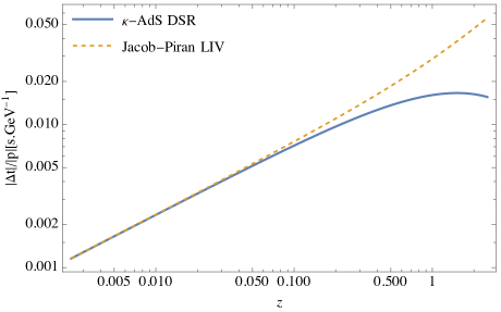
Figure 3: Ratio between the absolute value of time delay in cosmological coordinates and the hard photon’s momentum, as function of the redshift, for $\ell^{-1}=E_{\text{Planck}}=1.2\times 10^{19}\,\text{GeV}$, $\lambda=5\times 10^{-18}\,\text{s}^{-1}$. The blue/solid line describes the $\kappa$-AdS time delay given by Eq.(59) without MDR and just with relative locality effects. While the orange/dashed line describes a completely differenc scenario, with a MDR in cosmological coordinates and we depict only the time delay of the Jacob-Piran formula (61).

The accelerated expansion of the universe implies that for small redshifts we can actually describe the spacetime geometry by a de Sitter metric and the $\kappa$-de Sitter algebra could actually be used to constrain the quantum gravity parameter at the dark energy dominated epoch. But we cannot say the same of our case. There is no evidence that we have had an anti-de Sitter epoch in the universe, which in fact, has some unphysical features, like the existence of closed timelike curves, besides other features, like the absence of Cauchy surfaces (see section 5.2 of Hawking:1973uf ). Nevertheless, the main point of this paper is the construction of a time delay from deformation of translations in a class of quantum algebras that was not explored before to derive this observable. We expect that in the future we can use these results as a starting point to construct a more realistic scenario that glues pieces of anti-de Sitter propagation to construct an FLRW-based time delay that is compatible with the DSR principles in a similar way of what was done in Rosati:2015pga for the $\kappa$-de Sitter case, in order to extend the class of DSR-inspired time delays formulas.

VI Final Remarks

We found the relation between the generators of the $\kappa$-anti-de Sitter algebra in $1+1$ dimensions Ballesteros:2016bml and the undeformed anti-de Sitter algebra at first order in the quantum gravity parameter. We found that in the basis used in Ballesteros:2016bml , the boost and spacetime translations are deformed. However, we discovered that there is no deformation of the Casimir charge when we express it in terms of the undeformed quantities. This means that the trajectories are undeformed at first order of correction.

In a Lorentz invariance violating scenario, this means that the presence of classical trajectories implies in the absence of a time delay when particles with different energies are emitted simultaneously in a distant source and detected on earth Addazi:2021xuf . However, if we assume that the relativity principle is preserved, i.e., that the the local frames of the emission of the detection events are related by a deformed translation, then a reminiscent first order effect remains. This result has been derived using the $\kappa$-de Sitter algebra in the past Amelino-Camelia:2012vzf . However for the first time, we perform a derivation using the $\kappa$-anti-de Sitter algebra.

A novel result is the emergence of a sinusoidal time delay, which is related to the oscillatory behavior of the anti-de Sitter spacetime, which is a property that is evident in cosmological coordinates, but it is in fact a coordinate-independent feature of this geometry, as discussed in section 5.2 of Hawking:1973uf . Since the time delays phenomenology is based on the $\Lambda$-CDM cosmology, which does not present an anti-de Sitter epoch Staicova:2023vln ; Staicova:2024ljn , we do not envisage a direct applications of this result to observations.

Nevertheless, the $\kappa$-de Sitter results has been used as the cornerstone for the derivation of a time delay formula that would be compatible with local relativistic principles, through the creative construction of a propagation of signals and communication frames in a quantum FLRW spacetime by infinitesimal delays based on $\kappa$-de Sitter algebra with different curvatures Rosati:2015pga . Since there is no privileged role of positive curvature in comparison to the negative one from the geometric and algebraic perspectives, we wonder what kind of result would be found had one used the $\kappa$-AdS algebra as the fundamental bricks to build such delay in the effective FLRW spacetime.

The main challenge of this approach is how to handle the composition of coordinates of $\kappa$-AdS algebra which is given by trigonometric functions, while in $\kappa$-dS algebra the cosmological and conformal coordinates furnish computationally simpler functions. Despite these difficulties, a first and necessary step towards this analysis is the derivation of such delay for a single curvature, which was carried out in this paper. In the future, we aim to extend the results of this paper in two fronts: the exploration of different bases of $\kappa$-AdS algebra in order to derive more general results that include deformed trajectories; and to construct the effective FLRW time delay based on the $\kappa$-AdS algebra building bricks for the slicing technique.

References

- (1) C. Kiefer, Quantum gravity, vol. 124. Clarendon, Oxford, 2004.
- (2) J. Polchinski, String theory. Vol. 1: An introduction to the bosonic string. Cambridge Monographs on Mathematical Physics. Cambridge University Press, 12, 2007.
- (3) J. Polchinski, String theory. Vol. 2: Superstring theory and beyond. Cambridge Monographs on Mathematical Physics. Cambridge University Press, 12, 2007.
- (4) A. Ashtekar and E. Bianchi, “A short review of loop quantum gravity,” Rept. Prog. Phys. 84 (2021) no. 4, 042001, arXiv:2104.04394 [gr-qc].
- (5) R. Loll, “Quantum Gravity from Causal Dynamical Triangulations: A Review,” Class. Quant. Grav. 37 (2020) no. 1, 013002, arXiv:1905.08669 [hep-th].
- (6) A. Eichhorn, “An asymptotically safe guide to quantum gravity and matter,” Front. Astron. Space Sci. 5 (2019) 47, arXiv:1810.07615 [hep-th].
- (7) G. Amelino-Camelia, “Quantum-Spacetime Phenomenology,” Living Rev. Rel. 16 (2013) 5, arXiv:0806.0339 [gr-qc].
- (8) A. Addazi et al., “Quantum gravity phenomenology at the dawn of the multi-messenger era—A review,” Prog. Part. Nucl. Phys. 125 (2022) 103948, arXiv:2111.05659 [hep-ph].
- (9) Fermi GBM/LAT Collaboration, M. Ackermann et al., “A limit on the variation of the speed of light arising from quantum gravity effects,” Nature 462 (2009) 331–334, arXiv:0908.1832 [astro-ph.HE].
- (10) R. Alves Batista et al., “White Paper and Roadmap for Quantum Gravity Phenomenology in the Multi-Messenger Era,” arXiv:2312.00409 [gr-qc].
- (11) R. Gambini and J. Pullin, “Nonstandard optics from quantum space-time,” Phys. Rev. D 59 (1999) 124021, arXiv:gr-qc/9809038.
- (12) G. Amelino-Camelia, M. M. da Silva, M. Ronco, L. Cesarini, and O. M. Lecian, “Spacetime-noncommutativity regime of Loop Quantum Gravity,” Phys. Rev. D 95 (2017) no. 2, 024028, arXiv:1605.00497 [gr-qc].
- (13) V. A. Kostelecky, “Gravity, Lorentz violation, and the standard model,” Phys. Rev. D 69 (2004) 105009, arXiv:hep-th/0312310.
- (14) U. Jacob and T. Piran, “Lorentz-violation-induced arrival delays of cosmological particles,” JCAP 01 (2008) 031, arXiv:0712.2170 [astro-ph].
- (15) J. R. Ellis, N. E. Mavromatos, D. V. Nanopoulos, and A. S. Sakharov, “Quantum-gravity analysis of gamma-ray bursts using wavelets,” Astron. Astrophys. 402 (2003) 409–424, arXiv:astro-ph/0210124.
- (16) G. Amelino-Camelia, A. Marciano, M. Matassa, and G. Rosati, “Deformed Lorentz symmetry and relative locality in a curved/expanding spacetime,” Phys. Rev. D 86 (2012) 124035, arXiv:1206.5315 [hep-th].
- (17) G. Rosati, G. Amelino-Camelia, A. Marciano, and M. Matassa, “Planck-scale-modified dispersion relations in FRW spacetime,” Phys. Rev. D 92 (2015) no. 12, 124042, arXiv:1507.02056 [hep-th].
- (18) G. Amelino-Camelia, G. Rosati, and S. Bedić, “Phenomenology of curvature-induced quantum-gravity effects,” Phys. Lett. B 820 (2021) 136595, arXiv:2012.07790 [gr-qc].
- (19) G. Amelino-Camelia, M. G. Di Luca, G. Gubitosi, G. Rosati, and G. D’Amico, “Could quantum gravity slow down neutrinos?,” Nature Astron. 7 (2023) no. 8, 996–1001, arXiv:2209.13726 [gr-qc].
- (20) G. Amelino-Camelia, D. Frattulillo, G. Gubitosi, G. Rosati, and S. Bedić, “Phenomenology of DSR-relativistic in-vacuo dispersion in FLRW spacetime,” arXiv:2307.05428 [gr-qc].
- (21) C. Pfeifer, “Redshift and lateshift from homogeneous and isotropic modified dispersion relations,” Phys. Lett. B 780 (2018) 246–250, arXiv:1802.00058 [gr-qc].
- (22) J. Bolmont et al., “First Combined Study on Lorentz Invariance Violation from Observations of Energy-dependent Time Delays from Multiple-type Gamma-Ray Sources. I. Motivation, Method Description, and Validation through Simulations of H.E.S.S., MAGIC, and VERITAS Data Sets,” Astrophys. J. 930 (2022) no. 1, 75, arXiv:2201.02087 [astro-ph.HE].
- (23) G. Amelino-Camelia, “Relativity in space-times with short distance structure governed by an observer independent (Planckian) length scale,” Int. J. Mod. Phys. D 11 (2002) 35–60, arXiv:gr-qc/0012051.
- (24) G. Amelino-Camelia, L. Freidel, J. Kowalski-Glikman, and L. Smolin, “The principle of relative locality,” Phys. Rev. D 84 (2011) 084010, arXiv:1101.0931 [hep-th].
- (25) R. Schutzhold and W. G. Unruh, “Large-scale nonlocality in ’doubly special relativity’ with an energy-dependent speed of light,” JETP Lett. 78 (2003) 431–435, arXiv:gr-qc/0308049.
- (26) S. Hossenfelder, “Bounds on an energy-dependent and observer-independent speed of light from violations of locality,” Phys. Rev. Lett. 104 (2010) 140402, arXiv:1004.0418 [hep-ph].
- (27) G. Amelino-Camelia, M. Arzano, J. Kowalski-Glikman, G. Rosati, and G. Trevisan, “Relative-locality distant observers and the phenomenology of momentum-space geometry,” Class. Quant. Grav. 29 (2012) 075007, arXiv:1107.1724 [hep-th].
- (28) A. Ballesteros, F. J. Herranz, F. Musso, and P. Naranjo, “The -(A)dS quantum algebra in (3+1) dimensions,” Phys. Lett. B 766 (2017) 205–211, arXiv:1612.03169 [hep-th].
- (29) A. Ballesteros, G. Gubitosi, and F. Mercati, “Interplay between Spacetime Curvature, Speed of Light and Quantum Deformations of Relativistic Symmetries,” Symmetry 13 (2021) no. 11, 2099, arXiv:2110.04867 [gr-qc].
- (30) J. Magueijo and A. Mozaffari, “Simple generalizations of anti-deSitter space-time,” Class. Quant. Grav. 27 (2010) 135004, arXiv:0911.3697 [gr-qc].
- (31) J. M. Carmona, J. L. Cortés, J. J. Relancio, and M. A. Reyes, “Time delays, choice of energy-momentum variables, and relative locality in doubly special relativity,” Phys. Rev. D 106 (2022) no. 6, 064045, arXiv:2207.03799 [gr-qc].
- (32) S. W. Hawking and G. F. R. Ellis, The Large Scale Structure of Space-Time. Cambridge Monographs on Mathematical Physics. Cambridge University Press, 2, 2023.
- (33) D. Staicova, “Impact of cosmology on Lorentz Invariance Violation constraints from GRB time-delays,” Class. Quant. Grav. 40 (2023) no. 19, 195012, arXiv:2305.06504 [gr-qc].
- (34) D. Staicova, “Probing for Lorentz Invariance Violation in Pantheon Plus Dominated Cosmology,” arXiv:2401.06068 [gr-qc].