A globalization of L-BFGS for nonconvex unconstrained optimization

Abstract

We present a modification of the limited memory BFGS (L-BFGS) method that ensures global and linear convergence on nonconvex objective functions. Importantly, the modified method turns into classical L-BFGS if its iterates cluster at a point near which the objective is strongly convex with Lipschitz continuous gradients, inheriting the effectiveness of the classical method. These results, which are not available for existing modified L-BFGS methods, are facilitated by a novel form of cautious updating [LF01b]. The new updating mechanism involves a dynamic handling of the stored update vectors, where it is decided anew in each iteration which of the stored pairs are used for updating and which ones are skipped. The convergence analysis is carried out in infinite dimensional Hilbert space and contains several improvements of the convergence theory of L-BFGS-type methods. The results of this work also hold if the memory size in the modified L-BFGS method is zero, in which case the method is a Barzilai–Borwein method with cautious updating. As for L-BFGS, this is the first globalization with the desirable trait that it turns into its unmodified counterpart when its iterates cluster at a suitable point. We also prove that the Wolfe–Powell conditions induce global convergence if the gradient of the objective is continuous, which is likely to be of independent interest. The numerical experiments indicate that if the parameters of the cautious updating are suitably chosen, the modified method agrees with its classical counterpart, suggesting that the classical method is inherently cautious. An implementation of the method is available on arXiv.

Mathematics Subject Classification (2020). 65J22, 65K05, 65K10, 90C06, 90C26, 90C30, 90C48, 90C53, 90C90

1 Introduction

L-BFGS [Noc80, LN89, BNS94] is one of the most most widely used methods for large-scale unconstrained optimization problems. In this paper, we study a globally convergent version of L-BFGS for the problem

$$\min_{x\in{\cal X}}\,f(x),$$ (P)

where $f:{\cal X}\rightarrow\mathbb{R}$ is continuously differentiable and bounded below, and ${\cal X}$ is a Hilbert space. The significance of the new method is given by its desirable convergence properties:

• every cluster point is stationary, cf. Theorem 4.11;

• $\lim_{k\to\infty}\lVert\nabla f(x_{k})\rVert=0$ if $\nabla f$ is uniformly continuous in some level set, cf. Theorem 4.10;

• if the iterates cluster at a point near which $f$ is strongly convex and $\nabla f$ is Lipschitz, then the iterates converge to this point at a linear rate and the method agrees with classical L-BFGS after a finite number of iterations, cf. Theorem 4.22 and Theorem 4.20.

To the best of our knowledge, this is the first method that converges globally for nonconvex objective functions while also recovering the original L-BFGS method under local strong convexity. The latter ability ensures that it will often inherit the supreme efficiency of L-BFGS. The convergence results and the transition to classical L-BFGS rely on a new form of cautious updates [LF01b] that we introduce in Section 3. We stress that the modifications to L-BFGS that we propose in this paper are fully compatible with the techniques used in efficient numerical realizations of L-BFGS. In particular, the modified method can still be implemented matrix free based on the well-known two-loop recursion. For practical purposes we note that the results of this work hold under the Wolfe–Powell conditions and also for backtracking line searches based on the Armijo condition.

In the numerical experiments the modified method agrees entirely with classical L-BFGS if one of its algorithmic parameters is chosen sufficiently small. This suggests that the classical method may be inherently cautious. In Remark 4.21 we comment further on this issue. An implementation of the method is freely available on arXiv.

Our convergence analysis includes the possibility that the memory size in L-BFGS is zero, in which case the new method becomes a globalized Barzilai–Borwein method [BB88, Ray97, DL02, DF05, DHSZ06, Dai13a]. Barzilai–Borwein-type methods have recently received renewed interest, cf. e.g. [DABY15, DKPS15, BDH19, DHL19, AK20, LMP21, AK22, CPRZ23, GO23, AB23]. Since our results are stronger than the available ones for nonconvex $f$, cf. the discussion in Section 1.1, the techniques and results in this paper are also of interest in the context of Barzilai–Borwein methods. That being said, nonmonotone line searches, which are understood to be more efficient for Barzilai–Borwein-type methods [AK20], are only addressed in the numerical experiments in Section 5, but not in the convergence analysis.

The analysis underlying Theorem 4.11 is of interest in its own right because it shows that the Wolfe–Powell conditions ensure global convergence if $\nabla f$ is continuous. It seems that this is the first time that the Wolfe–Powell conditions are analyzed without Lipschitz continuity of $\nabla f$. The proof relies on a simple but apparently new generalization of the Zoutendijk condition, cf. Lemma 4.6, which is valid for arbitrary descent directions. In turn, the global convergence result actually applies to a large class of descent methods, although we do not make this explicit.

Assumptions that frequently appear in the convergence analysis of L-BFGS-type methods are that $\nabla f$ is Lipschitz continuous in the level set $\Omega$ associated to the initial point, that $\Omega$ is bounded and that $f$ is twice continuously differentiable; cf. [LN89, ABGP14, KD15, BBEM19, BJRT22, TSY22], for instance. We will make none of these assumptions. This enables us to show in Theorem 4.22 that the new method converges globally and linearly if $f$ is continuously differentiable and bounded below, and if $(x_{k})$ has a cluster point near which $f$ is strongly convex and $\nabla f$ is Lipschitz.

Another improvement in Theorem 4.22 concerns the type of linear convergence. The strongest available result for the original L-BFGS method is the classical [LN89, Theorem 7.1], where it is shown that $(f(x_{k}))$ converges q-linearly and $(x_{k})$ converges r-linearly. We obtain the same rate for $(f(x_{k}))$, but for $(x_{k})$ we prove a stronger error estimate that implies $l$-step q-linear convergence for all sufficiently large $l$. A sequence that converges $l$-step q-linearly for a single $l$ is r-linearly convergent, but not vice versa. We discuss $l$-step q-linear convergence further in Section 4.4. Moreover, we show that $(\nabla f(x_{k}))$ satisfies a similar error estimate. We are not aware of works on L-BFGS that involve multi-step q-linear convergence, but it frequently appears in local results for Barzilai–Borwein methods, e.g. [DL02, AK20]. We establish the improved rates for the modified method in Theorem 4.22 under the aforementioned assumptions. In addition, we infer that if $f$ is strongly convex in $\Omega$, then the result also holds for classical L-BFGS, cf. Remark 4.23. This improves [LN89, Theorem 7.1] by lowering its assumptions while sharpening its conclusion.

There are few works that provide a convergence analysis of L-BFGS in Hilbert space. In fact, a Hilbert space setting is only considered in our work [MAM23] for a structured L-BFGS method and in [AK20, AK22, AB23] for the Barzilai–Borwein method. For BFGS, characterizations of the update and convergence analyses are available in Hilbert space, e.g., in [Gri86, GL89, MQ80, GS81, Kup96, VPP20]. Studying L-BFGS in Hilbert space is valuable because when the (globalized) L-BFGS method is applied to a discretization of an infinite dimensional optimization problem, its numerical performance is usually closely related to the convergence properties of the method on the infinite dimensional level. This relationship appears, for instance, in the form of mesh independence principles [ABPR86, KS87, HU04, AK22]. In Section 5 we validate the method’s mesh independence numerically for an optimal control problem.

1.1 Related literature

While it has long been known that L-BFGS converges at a linear rate from arbitrary starting points for strongly convex objectives [LN89, Theorem 7.1], convergence results for the nonconvex case are not available for the original method, and for the BFGS method there exist counterexamples [Dai02, Mas04, Dai13b] that show divergence for different line searches. As a consequence, various types of modifications have been developed for BFGS and L-BFGS to obtain global convergence for nonconvex objectives. For line search based methods we are aware of cautious updating [LF01b, WLQ06, WHZ12, BJRT22, YZZ22, LWH22], modified updating [LF01a, XLW13, KD15, YWS20], damped updating [Pow78, Gri91, ABGP14, Sch16] and modification of the line search [YWL17, HD20, YLL22]. Other options for globalization include trust region approaches, cf. [LBL02, BGZY17, BBEM19, BMPS22] and the references therein, iterative regularization, cf. [Liu14, TP15, TSY22, KS23], as well as robust BFGS [Yan22]. For Barzilai–Borwein methods global and linear convergence in a nonconvex setting is shown in [DL02, AB23]. However, there is no L-BFGS-type method available for nonconvex objectives that converges globally in the sense that every cluster point is stationary while also recovering classical L-BFGS under local strong convexity. Additional differences to the literature are summarized as follows.

• Global convergence is often established as $\liminf_{k\to\infty}\lVert\nabla f(x_{k})\rVert=0$, e.g. [LF01a, XLW13, KD15, YWS20, YZZ22]; this does not guarantee that every cluster point of $(x_{k})$ is stationary.

• If rate of convergence results are provided, they frequently rely on assumptions whose satisfaction is unclear in the nonconvex case; examples include $\lim_{k\to\infty}\lVert x_{k+1}-x_{k}\rVert=0$ in [LF01b, Theorem 3.5], convergence of $(x_{k})$ in [YZZ22, Theorem 3.2] and [DL02, Section 3], or the existence of $c>0$ such that $y_{k}^{T}s_{k}>c\lVert y_{k}\rVert\lVert s_{k}\rVert$ for all $k$ in [BBEM19, Theorem 3.2]. In particular, it is not clear that these assumptions hold if $\liminf_{k\to\infty}\lVert\nabla f(x_{k})\rVert=0$, $(x_{k})\subset\mathbb{R}^{N}$ is bounded, and $f$ is $C^{\infty}$ with a single stationary point that satisfies sufficient optimality conditions and that is the unique global minimizer.

• Some methods rely on beforehand knowledge of the local modulus of strong convexity. This comprises, for instance, methods that skip the update if $y_{k}^{T}s_{k}\geq\mu\lVert s_{k}\rVert^{2}$ is violated, where $\mu>0$ is chosen at the beginning of the algorithm, e.g. [BJRT22, MAM23], which is a type of cautious updating. Clearly, if $f$ is strongly convex and $\mu$ is no larger than the modulus of strong convexity, all updates are carried out (as in L-BFGS). On the other hand, if $\mu$ is too large, all updates may be skipped, which will usually diminish the efficiency significantly. This problem persists in nonconvex situations even if $(x_{k})$ converges to a stationary point near which $f$ is strongly convex. In globalized Barzilai–Borwein methods and L-BFGS with seed matrices $H_{0}^{(k)}=\gamma_{k}I$, this issue (also) arises when the step sizes, respectively, the scaling factors $(\gamma_{k})$ are safeguarded away from zero, e.g. in [AB23]. These issues do not appear in the modified cautious updates because we replace $\mu$ by a null sequence $(\mu_{k})$ and allow $(\gamma_{k})$ to approach zero. In turn, we can show that our method turns into classical L-BFGS under local strong convexity of $f$ regardless of the local modulus of strong convexity.

1.2 Organization and notation

The paper is organized as follows. Section 2 recalls the classical L-BFGS method. In Section 3 we present the modified L-BFGS method. Its convergence is studied in Section 4. Section 5 contains numerical experiments and Section 6 concludes with a summary.

Notation. We use $\mathbb{N}=\{1,2,3,\ldots\}$ and $\mathbb{N}_{0}=\mathbb{N}\cup\{0\}$. The scalar product of $x,y\in{\cal X}$ is indicated by $x^{T}y$. For $x\in{\cal X}$ the linear functional $y\mapsto x^{T}y$ is denoted by $x^{T}$. We write $M\in\mathcal{L}({\cal X})$ if $M:{\cal X}\rightarrow{\cal X}$ is a bounded linear operator with respect to the operator norm. An $M\in\mathcal{L}({\cal X})$ is self-adjoint iff it satisfies $x^{T}My=(Mx)^{T}y$ for all $x,y\in{\cal X}$. It is positive definite, respectively, positive semi-definite iff it is self-adjoint and there exists $\beta>0$, respectively, $\beta\geq 0$ such that $x^{T}Mx\geq\beta\lVert x\rVert^{2}$ for all $x\in{\cal X}\setminus\{0\}$. We set $\mathcal{L}_{+}({\cal X}):=\{M\in\mathcal{L}({\cal X}):\,M\text{ is positive definite}\}$.

2 The classical L-BFGS method

In this section we discuss the aspects of the classical L-BFGS method for Eq. P that are relevant to this work. The pseudo code of the method is given below as Algorithm 1.

Input: $x_{0}\in{\cal X}$, $m\in\mathbb{N}_{0}$

1 Let ${\cal I}:=\emptyset$

2 for $k=0,1,2,\ldots$ do

3       if $\lVert\nabla f(x_{k})\rVert=0$ then $output$ $x_{k}$ and $break$

       Choose $H_{k}^{(0)}\in\mathcal{L}_{+}({\cal X})$

        // Often, $H_{k}^{(0)}=\gamma_{k}I$ for some $\gamma_{k}>0$

4       Compute $d_{k}:=-H_{k}\nabla f(x_{k})$ from $H_{k}^{(0)}$ and the stored pairs $\{(s_{j},y_{j})\}_{j\in{\cal I}}$

5       Compute step size $\alpha_{k}>0$

6       Compute $s_{k}:=\alpha_{k}d_{k}$, $x_{k+1}:=x_{k}+s_{k}$, $y_{k}:=\nabla f(x_{k+1})-\nabla f(x_{k})$

7       if $y_{k}^{T}s_{k}>0$ then append $(s_{k},y_{k})$ to storage and redefine ${\cal I}:={\cal I}\cup\{k\}$

8       if $\lvert{\cal I}\rvert>m$ then let $n:=\min\,{\cal I}$, remove $(s_{n},y_{n})$ from storage and redefine ${\cal I}:={\cal I}\setminus\{n\}$

9      

10 end for

Algorithm 1 Inverse L-BFGS method

The L-BFGS operator $\mathbf{H_{k}}$

We recall the definition of the operator $H_{k}$ appearing in Algorithm 1. It is easy to see that $\lvert{\cal I}\rvert\leq m$ holds in Algorithm 1 for any $k$, so there is $r=r(k)$ with $0\leq r\leq m$ such that ${\cal I}=\{k_{0},k_{1},\ldots,k_{r-1}\}\subset\mathbb{N}_{0}$. If ${\cal I}=\emptyset$, we let $H_{k}:=H_{k}^{(0)}$. Otherwise, we simplify notation by identifying $k_{j}$ with $j$ for $j=0,\ldots,r-1$. That is, ${\cal I}=\{0,1,\ldots,r-1\}$ and the storage is given by $\{(s_{j},y_{j})\}_{j=0}^{r-1}$ with $y_{j}^{T}s_{j}>0$ for $j=0,\ldots,r-1$ (since $(s_{k},y_{k})$ is only stored if $y_{k}^{T}s_{k}>0$). Endowed with this notation, the operator $H_{k}$ is obtained as $H_{k}:=H_{k}^{(r)}$ from the seed matrix $H_{k}^{(0)}$ and the storage $\{(s_{j},y_{j})\}_{j\in{\cal I}}$ by means of the recursion

$$H_{k}^{({j+1})}=V_{j}^{T}H_{k}^{(j)}V_{j}+\rho_{j}s_{j}s_{j}^{T},\qquad j=0,\ldots,r-1,$$ (1)

where $V_{j}:=I-\rho_{j}y_{j}s_{j}^{T}$ and $\rho_{j}:=(y_{j}^{T}s_{j})^{-1}$. From the Sherman–Morrison formula we infer that $B_{k}=H_{k}^{-1}$ can be obtained by setting $B_{k}:=B_{k}^{(r)}$ in the recursion

$$B_{k}^{(j+1)}:=B_{k}^{(j)}-\frac{B_{k}^{(j)}s_{j}(B_{k}^{(j)}s_{j})^{T}}{(B_{k}^{(j)}s_{j})^{T}s_{j}}+\frac{y_{j}y_{j}^{T}}{y_{j}^{T}s_{j}},\qquad j=0,\ldots,r-1,$$

where $B_{k}^{(0)}:=(H_{k}^{(0)})^{-1}$. In practice we do not form $H_{k}$, but compute the search direction $d_{k}=-H_{k}\nabla f(x_{k})$ in a matrix free way through the two-loop recursion [NW06, Algorithm 7.4]. This computation is very efficient, enabling the use of L-BFGS for large-scale problems.

Choice of the seed matrix $\mathbf{H_{k}^{(0)}}$

The most common choice is $H_{k}^{(0)}=\gamma_{k}I$, where

$$\gamma_{k}=\frac{y_{k-1}^{T}s_{k-1}}{\lVert y_{k-1}\rVert^{2}},$$ (2)

cf. [NW06, (7.20)], but other choices of $\gamma_{k}$ and of $H_{k}^{(0)}$ have also been studied, e.g. in [Ore82, LN89, GL89] and [ML13, DM19, And21]. In particular, the following two values are well-known choices for $\gamma_{k+1}$ (the index shift is for later reference).

Definition 2.1.

Let $k\in\mathbb{N}_{0}$ and let $(s_{k},y_{k})\in{\cal X}\times{\cal X}$ with $y_{k}^{T}s_{k}>0$. We set

$$\gamma_{k+1}^{-}:=\frac{y_{k}^{T}s_{k}}{\lVert y_{k}\rVert^{2}}\qquad\text{ and }\qquad\gamma_{k+1}^{+}:=\frac{\lVert s_{k}\rVert^{2}}{y_{k}^{T}s_{k}}.$$

To simplify the presentation of the modified L-BFGS method in Section 3, we restrict attention to choices of the form $H_{k}^{(0)}=\gamma_{k}I$ with $\gamma_{k}\in[\gamma_{k}^{-},\gamma_{k}^{+}]$. For memory size $m=0$ this yields $d_{k}=-\gamma_{k}\nabla f(x_{k})$, which shows that in this case Algorithm 1 may be viewed as a globalized Barzilai–Borwein method. For Barzilai–Borwein methods, the values $\gamma_{k}^{-}$ and $\gamma_{k}^{+}$ were introduced in [BB88]. The restriction $\gamma_{k}\in[\gamma_{k}^{-},\gamma_{k}^{+}]$ appears for instance in the spectral gradient methods of [DHL19], which provides ample references to related Barzilai–Borwein methods.

Remark 2.2.

The Cauchy–Schwarz inequality implies $\gamma_{k+1}^{-}\leq\gamma_{k+1}^{+}$. Furthermore, it is well-known that for twice differentiable $f$ with positive definite Hessians, the numbers $\gamma_{k+1}^{-}$ and $\gamma_{k+1}^{+}$ fall within the spectrum of the inverse of the averaged Hessian $\int_{0}^{1}\nabla^{2}f(x_{k}+ts_{k})\mathrm{d}t$, cf. [MAM23] for a statement in Hilbert space. If $f$ is quadratic with positive definite Hessian $B$, we have $Bs_{k}=y_{k}$, hence $\gamma_{k+1}^{+}$ is the inverse of a Rayleigh quotient of $B$ and $\gamma_{k+1}^{-}$ is a Rayleigh quotient of $B^{-1}$.

Choice of the step size $\boldsymbol{\alpha_{k}}$

Most often, Algorithm 1 is employed with a line search that ensures the satisfaction of the Wolfe–Powell conditions or the strong Wolfe–Powell conditions. That is, for constants $\sigma\in(0,1)$ and $\eta\in[\sigma,1)$, the step sizes $\alpha_{k}$ are selected in such a way that they satisfy the Armijo condition

$$f(x_{k+1})\leq f(x_{k})+\alpha_{k}\sigma\nabla f(x_{k})^{T}d_{k}$$ (3)

and either the curvature condition or the strong curvature condition

$$\nabla f(x_{k+1})^{T}d_{k}\geq\eta\nabla f(x_{k})^{T}d_{k}\qquad\text{ or }\qquad\left\lvert\nabla f(x_{k+1})^{T}d_{k}\right\rvert\leq\eta\left\lvert\nabla f(x_{k})^{T}d_{k}\right\rvert.$$ (4)

This entails that $y_{k}^{T}s_{k}>0$, so the current secant pair $(s_{k},y_{k})$ is guaranteed to enter the storage in Algorithm 1, which slightly simplifies the algorithm, e.g. [NW06, Algorithm 7.5], and ensures that the storage contains the most recent secant information. Since we also consider line searches that only involve the Armijo condition Eq. 3, we may have $y_{k}^{T}s_{k}\leq 0$. In this case the pair $(s_{k},y_{k})$ is not stored as using it in the construction of $H_{k+1}$ would result in $H_{k+1}$ not being positive definite. While this skipping of secant information seems undesirable, it can still pay off to work only with the Armijo condition; cf., e.g., [ACG18, MAM23]. If step sizes are based on Eq. 3 only, we demand that they are computed by backtracking. That is, if $\alpha_{k,i}$ does not satisfy Eq. 3, then the next trial step size $\alpha_{k,i+1}$ is chosen from $[\beta_{1}\alpha_{k,i},\beta_{2}\alpha_{k,i}]$, where $i=0,1,\ldots$, $\alpha_{k,0}:=1$ and $0<\beta_{1}\leq\beta_{2}<1$ are constants. This includes step size strategies that use interpolation, e.g. [DS96, Section 6.3.2].

Effect of update skipping on storage

If no new pair enters the storage in Algorithm 1, then no old pair will be removed in Algorithm 1, so we allow older information to be retained. Other variants are conceivable, e.g., we could always remove $(s_{k-m},y_{k-m})$ from the storage and set ${\cal I}:={\cal I}\setminus\{k-m\}$ in Algorithm 1. This would not affect the convergence analysis of this work in a meaningful way.

3 The modified L-BFGS method

Denoting

$$q:{\cal X}\times{\cal X}\rightarrow\mathbb{R},\qquad q(s,y):=\begin{cases}\min\left\{\frac{y^{T}s}{\lVert s\rVert^{2}},\,\frac{y^{T}s}{\lVert y\rVert^{2}}\right\}&\text{ if }s\neq 0\text{ and }y\neq 0,\\ 0&\text{ else},\end{cases}$$

the modified L-BFGS method is given as Algorithm 2 below.

Input: $x_{0}\in{\cal X}$, $m\in\mathbb{N}_{0}$, $c_{0}\in(0,1]$, $c_{1},c_{2}\in(0,\infty)$

  // Later we also require $c_{2}<1/(2m+2)$

1

2 Let ${\cal I}:=\emptyset$, $\gamma_{0}^{-}:=0$, $\gamma_{0}^{+}:=\infty$

3 for $k=0,1,2,\ldots$ do

4       if $\lVert\nabla f(x_{k})\rVert=0$ then $output$ $x_{k}$ and $break$

5       Let $\omega_{k}:=\min\{c_{0},c_{1}\lVert\nabla f(x_{k})\rVert^{c_{2}}\}$

6       Choose $\gamma_{k}\in[\gamma_{k}^{-},\gamma_{k}^{+}]\cap[\omega_{k},\omega_{k}^{-1}]$ if possible; else choose $\gamma_{k}\in[\omega_{k},\omega_{k}^{-1}]$

7       Let $H_{k}^{(0)}:=\gamma_{k}I$

8       Compute $d_{k}:=-H_{k}\nabla f(x_{k})$ from $H_{k}^{(0)}$ and the pairs in $\{(s_{j},y_{j})\}_{j\in{\cal I}}$ with $q(s_{j},y_{j})\geq\omega_{k}$

9       Compute step size $\alpha_{k}>0$

10       Compute $s_{k}:=\alpha_{k}d_{k}$, $x_{k+1}:=x_{k}+s_{k}$, $y_{k}:=\nabla f(x_{k+1})-\nabla f(x_{k})$

11       if $y_{k}^{T}s_{k}>0$  then

12            append $(s_{k},y_{k})$ to storage and redefine ${\cal I}:={\cal I}\cup\{k\}$

13             compute $\gamma_{k+1}^{-}$ and $\gamma_{k+1}^{+}$ according to Definition 2.1

14       else

15            let $\gamma_{k+1}^{-}:=0$ and $\gamma_{k+1}^{+}:=\infty$

16       end if

17      if $\lvert{\cal I}\rvert>m$ then let $n:=\min\,{\cal I}$, remove $(s_{n},y_{n})$ from storage and redefine ${\cal I}:={\cal I}\setminus\{n\}$

18      

19 end for

Algorithm 2 The modified inverse L-BFGS method

The interval $[\gamma_{k}^{-},\gamma_{k}^{+}]\cap[\omega_{k},\omega_{k}^{-1}]$ in Algorithm 2 is well-defined, but it may be empty. In that case, $[\omega_{k},\omega_{k}^{-1}]$ is used. The latter is nonempty due to $c_{0}\in(0,1]$. Further comments are as follows.

The two main novelties of Algorithm 2

While Algorithm 2 still stores any pair $(s_{k},y_{k})$ with $y_{k}^{T}s_{k}>0$, cf. Algorithm 2, it does not necessarily use all stored pairs for constructing $H_{k}$. Instead, in every iteration the updating involves only those of the stored pairs $(s_{j},y_{j})$, $j\in{\cal I}$, that satisfy $q(s_{j},y_{j})\geq\omega_{k}$, cf. Algorithm 2. We recall that the construction of $H_{k}$ is described in Section 2. Note that the condition $q(s_{j},y_{j})\geq\omega_{k}$ relates all stored pairs to the current value $\omega_{k}$, so a pair $(s_{j},y_{j})$ in the storage may be used to form $H_{k}$ in some iterations, but may be skipped in others, until it is removed from the storage. In contrast, in L-BFGS a pair within the storage is consistently used to form $H_{k}$ until it is removed from the storage. The second novelty concerns the choice of $\gamma_{k}$. In classical L-BFGS with Wolfe–Powell step sizes we have $\gamma_{k}^{-}>0$ for all $k$, so often $\gamma_{k}=\gamma_{k}^{-}$ is chosen for all $k$. By additionally requiring $\gamma_{k}\in[\omega_{k},\omega_{k}^{-1}]$, Algorithm 2 further restricts the choice of $\gamma_{k}$. In particular, this may prevent the choice $\gamma_{k}=\gamma_{k}^{-}$ for some $k$. The key point is that these two modifications allow us to bound $\lVert H_{k}\rVert$ and $\lVert H_{k}^{-1}\rVert$ in terms of $\omega_{k}$, cf. Lemma 4.4, which is crucial for establishing the global convergence of Algorithm 2 in Theorem 4.10 and Theorem 4.11 (note that $\omega_{k}$ is related to $\lVert\nabla f(x_{k})\rVert$).

Relation of Algorithm 2 to cautious updating

We emphasize that the two main novelties of Algorithm 2 are based on the cautious updating introduced by Li and Fukushima in [LF01b] for the BFGS method. There, the BFGS update based on $(s_{k},y_{k})$ is applied if $y_{k}^{T}s_{k}/\lVert s_{k}\rVert^{2}\geq\epsilon\lVert\nabla f(x_{k})\rVert^{\alpha}$ for positive constants $\epsilon$ and $\alpha$, otherwise the update is skipped; cf. [LF01b, (2.10)]. This condition for skipping the update has been employed many times in the literature, both for BFGS and for L-BFGS. However, to the best of our knowledge, in the existing variants once a pair $(s_{j},y_{j})$ is used for updating, it is also used for updating in every subsequent iteration (until it is removed from the storage in case of L-BFGS). Clearly, this is less flexible than deciding in each iteration which of the stored pairs are used for updating. Moreover, in classical cautious updating the decision whether to store a pair $(s_{j},y_{j})$ (and thus, to use it for updating) is based on $\lVert\nabla f(x_{j})\rVert$, whereas in Algorithm 2 the decision to involve a stored pair $(s_{j},y_{j})$ in the updating is based on the most recent norm $\lVert\nabla f(x_{k})\rVert$ rather than older norms. Finally, involving $\lVert\nabla f(x_{k})\rVert$ in the choice of $H_{k}^{(0)}$ seems to be new altogether apart from our very recent work [MAM23]. As it turns out, the novel form of cautious updating used in Algorithm 2 allows to bound $\lVert H_{k}\rVert$ and $\lVert H_{k}^{-1}\rVert$ in terms of $\lVert\nabla f(x_{k})\rVert^{-1}$, which is crucial for establishing global and linear convergence. We emphasize that the bounds for $\lVert H_{k}\rVert$ and $\lVert H_{k}^{-1}\rVert$ tend to infinity when $\lVert\nabla f(x_{k})\rVert$ tends to zero, cf. Lemma 4.4. This is highly desirable because it indicates that $\lVert H_{k}\rVert$ and $\lVert H_{k}^{-1}\rVert$ can become as large as necessary for $k\to\infty$, whereas any preset lower bound for $\gamma_{k}$ or $q(s_{k},y_{k})$ uniformly bounds the spectrum of $H_{k}$ and may therefore limit the ability of $H_{k}$ to capture the spectrum of the inverse Hessian, which would slow down the convergence.

Further novelties of Algorithm 2

If $\nabla f$ is Lipschitz in the level set associated to $x_{0}$, then $q$ can be replaced by the simpler function $\hat{q}(s,y):=y^{T}s/\lVert s\rVert^{2}$ for $s,y\neq 0$, $\hat{q}(s,y)=0$ else, without meaningfully affecting the convergence results of this paper. The decision criterion $\hat{q}(s_{j},y_{j})\geq\omega_{k}$ in Algorithm 2 of Algorithm 2 then resembles the original cautious updating more clearly. However, using $q$ instead of $\hat{q}$ enables global convergence if $\nabla f$ is continuous and linear convergence if $\nabla f$ is Lipschitz continuous near cluster points, cf. Theorem 4.11 and Theorem 4.22.

A possible generalization of Algorithm 2

Without meaningfully affecting the convergence theory of this paper we could replace the interval $[\gamma_{k}^{-},\gamma_{k}^{+}]$ in Algorithm 2 of Algorithm 2 by a larger interval $[\gamma_{k}^{\min},\gamma_{k}^{\max}]$, where $\gamma_{k}^{\min}:=\min\{c_{3},c_{4}\gamma_{k}^{-}\}$ and $\gamma_{k}^{\max}:=\max\{C_{3},C_{4}\gamma_{k}^{+}\}$ for constants $c_{3},c_{4},C_{3},C_{4}$. This allows, in particular, to include the choice $\gamma_{k}=1$ for all $k$, i.e., $H_{k}^{(0)}=I$, that also appears in the literature. However, in our assessment $H_{k}^{(0)}=\gamma_{k}I$ with $\gamma_{k}$ according to Eq. 2 is used much more often, so to keep the notation light we work with $[\gamma_{k}^{-},\gamma_{k}^{+}]$.

4 Convergence analysis

This section is devoted to the convergence properties of Algorithm 2. We start with its well-definedness in Section 4.1, after which we focus on the Wolfe–Powell line search in Section 4.2. Global and local convergence of Algorithm 2 are analyzed in Section 4.3 and Section 4.4.

4.1 Well-definedness

We recall some estimates to infer that Algorithm 2 is well-defined.

Lemma 4.1 (cf. [MAM23, Lemma 4.1]).

Let $M\in\mathbb{N}_{0}$ and $\kappa_{1},\kappa_{2}>0$. For all $j\in\{0,\ldots,M-1\}$ let $(s_{j},y_{j})\in{\cal X}\times{\cal X}$ satisfy

$$\frac{y_{j}^{T}s_{j}}{\lVert s_{j}\rVert^{2}}\geq\frac{1}{\kappa_{1}}\qquad\text{ and }\qquad\frac{y_{j}^{T}s_{j}}{\lVert y_{j}\rVert^{2}}\geq\frac{1}{\kappa_{2}}.$$

Moreover, let $H^{(0)}\in\mathcal{L}_{+}({\cal X})$. Then its L-BFGS update $H$, obtained from the recursion Eq. 1 using $H_{k}^{(0)}=H^{(0)}$ and $r=M$, satisfies $H\in\mathcal{L}_{+}({\cal X})$ and

$$\lVert H^{-1}\rVert\leq\lVert(H^{(0)})^{-1}\rVert+M\kappa_{2}$$ (5)

as well as

$$\lVert H\rVert\leq 5^{M}\max\bigl{\{}1,\lVert H^{(0)}\rVert\bigr{\}}\max\bigl{\{}1,\kappa_{1}^{M},(\kappa_{1}\kappa_{2})^{M}\bigr{\}}.$$ (6)

The following assumption ensures that Algorithm 2 is well-defined.

Assumption 4.2.

to enforce linebreak

1. The function $f:{\cal X}\rightarrow\mathbb{R}$ is continuously differentiable and bounded below.

2. The step size $\alpha_{k}$ in 2 either satisfies the Armijo condition Eq. 3 and is computed by backtracking for all $k$, or it satisfies the Wolfe–Powell conditions for all $k$, cf. Eq. 4.

Lemma 4.3.

Let Assumption 4.2 hold. Then Algorithm 2 either terminates for some $k\in\mathbb{N}_{0}$ in Algorithm 2 with an $x_{k}$ satisfying $\nabla f(x_{k})=0$ or it generates a sequence $(f(x_{k}))$ that is strictly monotonically decreasing and convergent.

Proof.

After observing that $[\omega_{k},\omega_{k}^{-1}]\neq\emptyset$ for all $k$ due to $c_{0}\leq 1$, the proof is similar to that of [MAM23, Lemma 4.5]. ∎

Applying Lemma 4.1 to Algorithm 2 yields the following result.

Lemma 4.4.

Let Assumption 4.2 hold and let $(x_{k})$ be generated by Algorithm 2. Then

$$\lVert H_{k}^{-1}\rVert\leq\left(\lVert I\rVert+m\right)\omega_{k}^{-1}\qquad\text{ and }\qquad\lVert H_{k}\rVert\leq 5^{m}\max\Bigl{\{}1,\omega_{k}^{-(2m+1)}\Bigr{\}}$$

are satisfied for all $k\in\mathbb{N}_{0}$, where $m$ is the constant from Algorithm 2.

Proof.

The acceptance criterion $q(s_{j},y_{j})\geq\omega_{k}$ in Algorithm 2 of Algorithm 2 implies that $y_{j}^{T}s_{j}/\lVert s_{j}\rVert^{2}\geq\omega_{k}$ and $y_{j}^{T}s_{j}/\lVert y_{j}\rVert^{2}\geq\omega_{k}$ for all $(s_{j},y_{j})$ that are involved in forming $H_{k}$. Moreover, Algorithm 2 ensures that $\omega_{k}\leq\gamma_{k}\leq\omega_{k}^{-1}$. Using Eq. 5, respectively, Eq. 6 we thus deduce that

$$\lVert H_{k}^{-1}\rVert\leq\lVert(H_{k}^{(0)})^{-1}\rVert+m\omega_{k}^{-1}=\lVert I\rVert\gamma_{k}^{-1}+m\omega_{k}^{-1}\leq\omega_{k}^{-1}\lVert I\rVert+m\omega_{k}^{-1}$$

and

$$\lVert H_{k}\rVert\leq 5^{m}\max\bigl{\{}1,\omega_{k}^{-1}\bigr{\}}\max\bigl{\{}1,\omega_{k}^{-2m}\bigr{\}}\leq 5^{m}\max\bigl{\{}1,\omega_{k}^{-(2m+1)}\bigr{\}}.\qed$$

The previous lemma implies useful bounds.

Corollary 4.5.

Let Assumption 4.2 hold and let $(x_{k})$ be generated by Algorithm 2. Then there are constants $c,C>0$ such that

$$c\min\Bigl{\{}1,\lVert\nabla f(x_{k})\rVert^{c_{2}}\Bigr{\}}\leq\frac{\lVert d_{k}\rVert}{\lVert\nabla f(x_{k})\rVert}\leq C\max\Bigl{\{}1,\lVert\nabla f(x_{k})\rVert^{-(2m+1)c_{2}}\Bigr{\}}$$ (7)

as well as

$$\frac{\lvert\nabla f(x_{k})^{T}d_{k}\rvert}{\lVert d_{k}\rVert}\geq c\lVert\nabla f(x_{k})\rVert\min\Bigl{\{}1,\lVert\nabla f(x_{k})\rVert^{2(m+1)c_{2}}\Bigr{\}}.$$

are satisfied for all $k\in\mathbb{N}_{0}$, where $c_{2}$ and $m$ are the constants from Algorithm 2.

Proof.

Since $d_{k}=-H_{k}\nabla f(x_{k})$, the estimates Eq. 7 readily follow from those for $\lVert H_{k}\rVert$ and $\lVert H_{k}^{-1}\rVert$. Concerning the final inequality we have

$$-\nabla f(x_{k})^{T}d_{k}=d_{k}^{T}H_{k}^{-1}d_{k}\geq\lVert d_{k}\rVert^{2}\lVert H_{k}\rVert^{-1}\\ \geq c\lVert d_{k}\rVert\lVert\nabla f(x_{k})\rVert\min\Bigl{\{}1,\lVert\nabla f(x_{k})\rVert^{(2m+2)c_{2}}\Bigr{\}},$$

where we used the first inequality of Eq. 7 and the estimate for $\lVert H_{k}\rVert$. ∎

4.2 A weaker form of the Zoutendijk condition for Wolfe–Powell line searches

To prove global convergence for step sizes that satisfy the Wolfe–Powell conditions, we will use the following result that establishes a less stringent form of the Zoutendijk condition. The advantage of the new condition is that it holds without Lipschitz continuity of the gradient, which is not true for the Zoutendijk condition, cf. e.g. [NW06, Theorem 3.2]. We recall that the curvature condition is the left one of the two inequalities in Eq. 4.

Lemma 4.6.

Let Assumption 4.2 hold and let $(x_{k})$, $(d_{k})$ and $(s_{k})$ be generated by Algorithm 2. Let $\nabla f$ be uniformly continuous in $\Omega=\{x\in{\cal X}:f(x)\leq f(x_{0})\}$. Let the curvature condition hold for all $k\in K$ and let $\lim_{K\ni k\to\infty}s_{k}=0$. Then $\lim_{K\ni k\to\infty}\frac{\lvert\nabla f(x_{k})^{T}d_{k}\rvert}{\lVert d_{k}\rVert}=0$.

Proof.

Since the algorithm has not terminated finitely, there holds $\nabla f(x_{k})\neq 0$ for all $k$, hence $d_{k}=-H_{k}\nabla f(x_{k})\neq 0$ for all $k$. From the curvature condition $\eta\nabla f(x_{k})^{T}d_{k}\leq\nabla f(x_{k+1})^{T}d_{k}$, $k\in K$, we infer

$$0\leq\left(\eta-1\right)\nabla f(x_{k})^{T}d_{k}\leq\bigl{[}\nabla f(x_{k}+s_{k})-\nabla f(x_{k})\bigr{]}^{T}d_{k},$$

where we used that $\eta\leq 1$ and $\nabla f(x_{k})^{T}d_{k}<0$. The Cauchy–Schwarz inequality yields

$$0\leq\left(1-\eta\right)\bigl{\lvert}\nabla f(x_{k})^{T}d_{k}\bigr{\rvert}\lVert d_{k}\rVert^{-1}\leq\lVert\nabla f(x_{k}+s_{k})-\nabla f(x_{k})\rVert$$

for all $k\in K$. Since $(x_{k})\subset\Omega$ and $\lim_{K\ni k\to\infty}s_{k}=0$, the uniform continuity of $\nabla f$ in $\Omega$ implies that the right-hand side converges to zero for $K\ni k\to\infty$. As $\eta\in(0,1)$, the claim follows. ∎

Remark 4.7.

It is easy to see that Lemma 4.6 also holds for continuous $\nabla f$ if we assume that $(x_{k})_{K}$ converges. It is also straightforward to confirm that Lemma 4.6 holds for sequences $(x_{k})$, $(d_{k})$ and $(s_{k})$ that are not generated by Algorithm 2 provided that $\nabla f(x_{k})^{T}d_{k}\leq 0$ for all $k$. We therefore expect Lemma 4.6 to be of considerable interest beyond this work.

4.3 Global convergence

In this section we establish that Algorithm 2 is globally convergent. In fact, we prove several types of global convergence under different assumptions.

The level set for Algorithm 2, respectively, the level set with $\delta$ vicinity are given by

$$\Omega:=\Bigl{\{}x\in{\cal X}:\;f(x)\leq f(x_{0})\Bigr{\}}\qquad\text{ and }\qquad\Omega_{\delta}:=\Omega+\mathbb{B}_{\delta}(0).$$

The first result relies on the following assumption.

Assumption 4.8.

to create linebreak

1. Assumption 4.2 holds.

2. The gradient of $f$ is uniformly continuous in $\Omega$, i.e., for all sequences $(x_{k})\subset\Omega$ and $(s_{k})\subset{\cal X}$ satisfying $(x_{k}+s_{k})\subset\Omega$ and $\lim_{k}s_{k}=0$, there holds $\lim_{k}\,\lVert\nabla f(x_{k}+s_{k})-\nabla f(x_{k})\rVert=0$.

3. If Algorithm 2 uses Armijo with backtracking to determine the step sizes, then there is $\delta>0$ such that $f$ or $\nabla f$ is uniformly continuous in $\Omega_{\delta}$.

Remark 4.9.

If ${\cal X}$ is finite dimensional and $\Omega$ is bounded (hence compact), 2) can be dropped since it follows from the continuity of $\nabla f$ included in Assumption 4.2. Similarly, the uniform continuity of $f$ or $\nabla f$ in $\Omega_{\delta}$ can be dropped if $\Omega_{\delta}$ is bounded and ${\cal X}$ is finite dimensional.

As a main result we show that Algorithm 2 is globally convergent under Assumption 4.8.

Theorem 4.10.

Let Assumption 4.8 hold. Then Algorithm 2 either terminates after finitely many iterations with an $x_{k}$ that satisfies $\nabla f(x_{k})=0$ or it generates a sequence $(x_{k})$ with

$$\lim_{k\to\infty}\,\lVert\nabla f(x_{k})\rVert=0.$$ (8)

In particular, every cluster point of $(x_{k})$ is stationary.

Proof.

The case that Algorithm 2 terminates is clear, so let us assume that it generates a sequence $(x_{k})$. If $(x_{k})$ satisfies Eq. 8, then by continuity it follows that every cluster point $x^{\ast}$ of $(x_{k})$ satisfies $\nabla f(x^{\ast})=0$. Hence, it only remains to establish Eq. 8. We argue by contradiction, so suppose that Eq. 8 were false. Then there is a subsequence $(x_{k})_{K}$ of $(x_{k})$ and an $\epsilon>0$ such that

$$\lVert\nabla f(x_{k})\rVert\geq\epsilon\qquad\forall k\in K.$$ (9)

Since $\alpha_{k}$ satisfies the Armijo condition for all $k\geq 0$, we infer from $-\nabla f(x_{k})^{T}d_{k}=d_{k}^{T}H_{k}^{-1}d_{k}$ that

$$\sigma\sum_{k\in K}\alpha_{k}\frac{\lVert d_{k}\rVert^{2}}{\lVert H_{k}\rVert}\leq-\sigma\sum_{k\in K}\alpha_{k}\nabla f(x_{k})^{T}d_{k}\leq\sum_{k\in K}\left[f(x_{k})-f(x_{k+1})\right]\leq\sum_{k=0}^{\infty}\left[f(x_{k})-f(x_{k+1})\right]<\infty,$$

where we used that $(f(x_{k}))$ is monotonically decreasing by Lemma 4.3. From Lemma 4.4 and Eq. 9 we obtain $\sup_{k\in K}\lVert H_{k}\rVert<\infty$, which yields $\sum_{k\in K}\alpha_{k}\lVert d_{k}\rVert^{2}<\infty$. From the first inequality in Eq. 7 and Eq. 9 we infer that

$$\exists c>0:\quad\lVert d_{k}\rVert\geq c\quad\forall k\in K.$$ (10)

Hence, $\sum_{k\in K}\alpha_{k}\lVert d_{k}\rVert^{2}<\infty$ implies $\sum_{k\in K}\alpha_{k}\lVert d_{k}\rVert<\infty$ and $\sum_{k\in K}\alpha_{k}<\infty$, thus

$$\lim_{K\ni k\to\infty}\alpha_{k}=\lim_{K\ni k\to\infty}s_{k}=0.$$ (11)

We now have to distinguish two cases depending on how the step sizes are determined.
Case 1: The step sizes are computed by Armijo with backtracking
From Eq. 11 and the construction of the backtracking we infer that for all sufficiently large $k\in K$ there is $\beta_{k}\in(0,\beta_{1}^{-1}]$ such that Eq. 3 is violated for $\hat{\alpha}_{k}:=\beta_{k}\alpha_{k}$. Therefore,

$$-\hat{\alpha}_{k}\sigma\nabla f(x_{k})^{T}d_{k}>f(x_{k})-f(x_{k}+\hat{\alpha}_{k}d_{k})=-\hat{\alpha}_{k}\nabla f(x_{k}+\theta_{k}\hat{\alpha}_{k}d_{k})^{T}d_{k}$$

for all these $k$ and $\theta_{k}\in(0,1)$. Multiplying by $-\hat{\alpha}_{k}^{-1}$ and subtracting $\nabla f(x_{k})^{T}d_{k}$ we obtain

$$(\sigma-1)\nabla f(x_{k})^{T}d_{k}<\left[\nabla f(x_{k}+\theta_{k}\hat{\alpha}_{k}d_{k})-\nabla f(x_{k})\right]^{T}d_{k}.$$

Due to $\sigma<1$ and $-\nabla f(x_{k})^{T}d_{k}=d_{k}^{T}H_{k}^{-1}d_{k}$ there holds for all $k\in K$ sufficiently large

$$(1-\sigma)\frac{\lVert d_{k}\rVert^{2}}{\lVert H_{k}\rVert}<\lVert\nabla f(x_{k}+\theta_{k}\hat{\alpha}_{k}d_{k})-\nabla f(x_{k})\rVert\lVert d_{k}\rVert.$$

Because of $h:=\sup_{k\in K}\lVert H_{k}\rVert<\infty$ this entails for all sufficiently large $k\in K$ that

$$(1-\sigma)\lVert d_{k}\rVert<h\lVert\nabla f(x_{k}+\theta_{k}\hat{\alpha}_{k}d_{k})-\nabla f(x_{k})\rVert.$$ (12)

As $\theta_{k}\in(0,1)$ and $\beta_{k}\leq\beta_{1}^{-1}$ for all $k\in K$, it follows from Eq. 11 that $\theta_{k}\hat{\alpha}_{k}d_{k}=\theta_{k}\beta_{k}s_{k}\to 0$ for $K\ni k\to\infty$. If $\nabla f$ is uniformly continuous in $\Omega_{\delta}$, then Eq. 12 implies $\lim_{K\ni k\to\infty}\lVert d_{k}\rVert=0$, which contradicts Eq. 10. If $f$ is uniformly continuous in $\Omega_{\delta}$, then $x_{k}+\theta_{k}\hat{\alpha}_{k}\lVert d_{k}\rVert\in\Omega$ for all large $k\in K$, so the uniform continuity of $\nabla f$ in $\Omega$ yields $\lim_{K\ni k\to\infty}\lVert d_{k}\rVert=0$ in Eq. 12 again, contradicting Eq. 10.
Case 2: The step sizes satisfy the Wolfe–Powell conditions
Combining Lemma 4.6 and Corollary 4.5 yields $\lim_{K\ni k\to\infty}\lVert\nabla f(x_{k})\rVert=0$, contradicting Eq. 9. ∎

Cluster points are already stationary under weaker assumptions than those of Theorem 4.10.

Theorem 4.11.

Let Assumption 4.2 hold and let $(x_{k})$ be generated by Algorithm 2. Then every cluster point of $(x_{k})$ is stationary.

Proof.

The proof is almost identical to that of Theorem 4.10. The main difference is that since the subsequence $(x_{k})_{K}$ now converges to some $x^{\ast}$, continuity of $f$ at $x^{\ast}$ implies that there is $\delta^{\prime}>0$ such that $\mathbb{B}_{\delta^{\prime}}(x^{\ast})\subset\Omega$ and for all sufficiently large $k\in K$ there holds $x_{k}\in\mathbb{B}_{\delta^{\prime}}(x^{\ast})$. Therefore, local assumptions in the vicinity of the cluster point suffice (e.g., continuity instead of uniform continuity). In Case 2 of the proof, in particular, we use Remark 4.7 instead of Lemma 4.6. ∎

If ${\cal X}$ is finite dimensional and $(x_{k})$ is bounded, we obtain the conclusions of Theorem 4.10 under the weaker assumptions of Theorem 4.11.

Corollary 4.12.

Let Assumption 4.2 hold and let $(x_{k})$ be generated by Algorithm 2. Let $(x_{k})$ be bounded and let ${\cal X}$ be finite dimensional. Then $(x_{k})$ has at least one cluster point, every cluster point is stationary, and $\lim_{k\to\infty}\lVert\nabla f(x_{k})\rVert=0$.

Proof.

The claims readily follow from Theorem 4.11. ∎

In the infinite dimensional case we additionally want weak cluster points to be stationary.

Lemma 4.13.

Let Assumption 4.2 hold and let $\nabla f$ be weak-to-weak continuous. Let $(x_{k})$ be generated by Algorithm 2 and let $\lim_{k\to\infty}\lVert\nabla f(x_{k})\rVert=0$. Then every weak cluster point of $(x_{k})$ is stationary.

Proof.

Let $x^{\ast}$ be a weak limit of $(x_{k})_{K}$. The weak-to-weak continuity of $\nabla f$ implies that $(\nabla f(x_{k}))_{K}$ weakly converges to $\nabla f(x^{\ast})$. Since $\lVert\cdot\rVert$ is weakly lower semicontinuous, it follows that

$$\lVert\nabla f(x^{\ast})\rVert\leq\liminf_{K\ni k\to\infty}\lVert\nabla f(x_{k})\rVert=\lim_{k\to\infty}\lVert\nabla f(x_{k})\rVert=0.\qed$$

Remark 4.14.

Assumption 4.8 is sufficient for $\lim_{k\to\infty}\lVert\nabla f(x_{k})\rVert=0$ to hold, cf. Theorem 4.10.

4.4 Linear convergence

In this section we prove that Algorithm 2 converges linearly under mild assumptions. More precisely, we show that $(f(x_{k}))$ converges q-linearly while $(x_{k})$ and $(\nabla f(x_{k}))$ satisfy estimates that imply $l$-step q-linear convergence for all sufficiently large $l$.

Definition 4.15.

We call $(x_{k})\subset{\cal X}$ $l$-step q-linearly convergent for some $l\in\mathbb{N}$, iff there exist $x^{\ast}\in{\cal X}$, $\bar{k}\geq 0$ and $\kappa\in(0,1)$ such that $\lVert x_{k+l}-x^{\ast}\rVert\leq\kappa\lVert x_{k}-x^{\ast}\rVert$ is satisfied for all $k\geq\bar{k}$.

For $l=1$ this is q-linear convergence. It is easy to see that $l$-step q-linear convergence for an arbitrary $l$ implies r-linear convergence whereas the opposite is not necessarily true.

We are not aware of works on BFGS-/L-BFGS-type methods that use the concept of $l$-step q-linear convergence. However, since Algorithm 2 also includes a Barzilai–Borwein-type method, we point out that the notion appears in [DL02, AK20, AK22] in convex and nonconvex settings.

The linear convergence of Algorithm 2 will be shown under the following assumption.

Assumption 4.16.

to create linebreak

1. Assumption 4.2 holds.

2. The constant $c_{2}$ in Algorithm 2 satisfies $c_{2}<(2m+1)^{-1}$ if the Armijo rule with backtracking is used, and $c_{2}<(2m+2)^{-1}$ else.

First we show that if a stationary cluster point $x^{\ast}$ belongs to a ball in which $f$ is strongly convex, then $x^{\ast}$ is attractive. It is crucial for this result that $c_{2}$ is chosen according to Assumption 4.16 2).

Lemma 4.17.

Let Assumption 4.16 hold and let $(x_{k})$ be generated by Algorithm 2. Let $(x_{k})$ have a cluster point $x^{\ast}$ with a convex neighborhood in which $f$ is strongly convex. Then $\lim_{k\to\infty}\lVert x_{k}-x^{\ast}\rVert=0$.

Proof.

We denote the neighborhood of $x^{\ast}$ by ${\cal N}$. The proof is divided into two parts.
Part 1: Cluster points induce vanishing steps
In this part of the proof we show that for all $\epsilon>0$ there exists a $\delta^{\prime}>0$ such that for any $k\in\mathbb{N}_{0}$ the implication $\lVert x_{k}-x^{\ast}\rVert<\delta^{\prime}\Rightarrow\lVert s_{k}\rVert<\epsilon$ holds true. Apparently, to prove this it suffices to consider only those $\epsilon$ that are so small that $\mathbb{B}_{\epsilon}(x^{\ast})\subset{\cal N}$ is satisfied. Let such an $\epsilon$ be given. From Corollary 4.5 we infer that for all $k\in\mathbb{N}_{0}$

$$\lVert d_{k}\rVert\leq C\lVert\nabla f(x_{k})\rVert^{1-(2m+1)c_{2}}.$$ (13)

The exponent in Eq. 13 is positive because of the assumption $c_{2}<(2m+1)^{-1}$, hence $\lVert d_{k}\rVert<\epsilon$ whenever $\lVert x_{k}-x^{\ast}\rVert<\delta^{\prime}$ for some sufficiently small $\delta^{\prime}>0$, where we used the continuity of $\nabla f$ at $x^{\ast}$ and $\nabla f(x^{\ast})=0$, which holds due to Theorem 4.11. If Algorithm 2 uses the Armijo rule with backtracking, then $\alpha_{k}\leq 1$ for all $k$, so the desired implication follows. In the remainder of Part 1 we can therefore assume that all $\alpha_{k}$, $k\in\mathbb{N}_{0}$, satisfy the Wolfe–Powell conditions. The strong convexity of $f$ in ${\cal N}$ implies the existence of $\mu>0$ such that

$$f(x)-f(x^{\ast})\leq\frac{1}{2\mu}\lVert\nabla f(x)\rVert^{2}$$

for all $x\in{\cal N}$. In particular, this holds for $x=x_{k}$ whenever $x_{k}\in\mathbb{B}_{\epsilon}(x^{\ast})$. Moreover, the Armijo condition Eq. 3 holds for all step sizes $\alpha_{k}$, $k\in\mathbb{N}_{0}$. Together, we have for all $k\in\mathbb{N}_{0}$ with $x_{k}\in\mathbb{B}_{\epsilon}(x^{\ast})$

$$\alpha_{k}\sigma\nabla f(x_{k})^{T}H_{k}\nabla f(x_{k})\leq f(x_{k})-f(x_{k+1})\leq f(x_{k})-f(x^{\ast})\leq\frac{1}{2\mu}\lVert\nabla f(x_{k})\rVert^{2},$$

where we used that $f(x_{k+1})\geq f(x^{\ast})$ as $(f(x_{k}))$ is monotonically decreasing. Thus, for these $k$

$$\alpha_{k}\leq\frac{\lVert H_{k}^{-1}\rVert}{2\sigma\mu}.$$

From Lemma 4.4 we obtain that $\lVert H_{k}^{-1}\rVert\leq\hat{C}\omega_{k}^{-1}$ for all $k\in\mathbb{N}_{0}$, where $\hat{C}>0$ is a constant. Decreasing $\delta^{\prime}$ if need be, we may assume $\delta^{\prime}\leq\epsilon$ and $\omega_{k}^{-1}=c_{1}^{-1}\lVert\nabla f(x_{k})\rVert^{-c_{2}}$ for all $k\in\mathbb{N}_{0}$ with $x_{k}\in\mathbb{B}_{\delta^{\prime}}(x^{\ast})$. Combining this with Eq. 13 we obtain for all $k\in\mathbb{N}_{0}$ with $x_{k}\in\mathbb{B}_{\delta^{\prime}}(x^{\ast})$ that

$$\lVert s_{k}\rVert=\alpha_{k}\lVert d_{k}\rVert\leq\frac{\lVert H_{k}^{-1}\rVert}{2\sigma\mu}\lVert d_{k}\rVert\leq\frac{C\hat{C}}{2\sigma\mu}\omega_{k}^{-1}\lVert\nabla f(x_{k})\rVert^{1-(2m+1)c_{2}}=\frac{C\hat{C}}{2\sigma\mu c_{1}}\lVert\nabla f(x_{k})\rVert^{1-2(m+1)c_{2}}.$$

The choice of $c_{2}$ in Assumption 4.16 2) implies that $1-2(m+1)c_{2}>0$. Thus, after decreasing $\delta^{\prime}$ if need be, there holds $\lVert s_{k}\rVert<\epsilon$ for all $k\in\mathbb{N}_{0}$ with $x_{k}\in\mathbb{B}_{\delta^{\prime}}(x^{\ast})$. This finishes the proof of Part 1.
Part 2: Convergence of the entire sequence $\mathbf{(x_{k})}$
Let $\epsilon^{\prime}>0$ be so small that $\mathbb{B}_{\epsilon^{\prime}}(x^{\ast})\subset{\cal N}$. We have to show that there is $\bar{k}\geq 0$ such that $x_{k}\in\mathbb{B}_{\epsilon^{\prime}}(x^{\ast})$ for all $k\geq\bar{k}$. Due to Part 1 we find a positive $\delta^{\prime}$ such that for all $k\in\mathbb{N}_{0}$ the implication $x_{k}\in\mathbb{B}_{\delta^{\prime}}(x^{\ast})\Rightarrow\lVert s_{k}\rVert<\epsilon^{\prime}/2$ holds true. Decreasing $\delta^{\prime}$ if need be, we can assume that $\delta^{\prime}\leq\epsilon^{\prime}/2$. It then follows that $x_{k+1}\in\mathbb{B}_{\epsilon^{\prime}}(x^{\ast})$ for all $k\in\mathbb{N}_{0}$ with $x_{k}\in\mathbb{B}_{\delta^{\prime}}(x^{\ast})$. Next we use that the $\mu$-strongly convex function $f|_{\mathbb{B}_{\epsilon^{\prime}}(x^{\ast})}$ satisfies the growth condition

$$f(x^{\ast})+\frac{\mu}{2}\lVert x-x^{\ast}\rVert^{2}\leq f(x)$$ (14)

for all $x$ in $\mathbb{B}_{\epsilon^{\prime}}(x^{\ast})$. Let $U:=\mathbb{B}_{\epsilon^{\prime}}(x^{\ast})\setminus\mathbb{B}_{\delta^{\prime}}(x^{\ast})$. Due to Eq. 14 we have $f(x)-f(x^{\ast})\geq(\delta^{\prime})^{2}\mu/2$ for all $x\in U$. Since $(f(x_{k}))$ converges by Lemma 4.3, we find $\hat{k}$ such that $f(x_{k})-f(x^{\ast})<(\delta^{\prime})^{2}\mu/2$ for all $k\geq\hat{k}$, hence $x_{k}\not\in U$ for all $k\geq\hat{k}$. Selecting $\bar{k}\geq\hat{k}$ such that $x_{\bar{k}}\in\mathbb{B}_{\delta^{\prime}}(x^{\ast})$, we obtain that $x_{\bar{k}+1}\in\mathbb{B}_{\epsilon^{\prime}}(x^{\ast})$ and $x_{\bar{k}+1}\not\in U$, thus $x_{\bar{k}+1}\in\mathbb{B}_{\delta^{\prime}}(x^{\ast})$. By induction we infer that $x_{k}\in\mathbb{B}_{\delta^{\prime}}(x^{\ast})$ for all $k\geq\bar{k}$, which concludes the proof as $\delta^{\prime}\leq\epsilon^{\prime}/2$. ∎

Next we show that $(\lVert H_{k}\rVert)$ and $(\lVert H_{k}^{-1}\rVert)$ are bounded under appropriate assumptions.

Lemma 4.18.

Let Assumption 4.2 hold and let $(x_{k})$ be generated by Algorithm 2. Suppose there are $x^{\ast}\in{\cal X}$ and a convex neighborhood ${\cal N}$ of $x^{\ast}$ such that $\lim_{k\to\infty}x_{k}=x^{\ast}$, $f|_{{\cal N}}$ is strongly convex and $\nabla f|_{{\cal N}}$ is Lipschitz. Then $(\lVert H_{k}\rVert)$ and $(\lVert H_{k}^{-1}\rVert)$ are bounded.

Proof.

Let $\bar{k}$ be such that $x_{k}\in{\cal N}$ for all $k\geq\bar{k}$. Since $f|_{{\cal N}}$ is strongly convex, there is $\mu>0$ such that $\nabla f$ is $\mu$-strongly monotone in ${\cal N}$, i.e.,

$$\bigl{[}\nabla f(\hat{x})-\nabla f(x)\bigr{]}^{T}(\hat{x}-x)\geq\mu\lVert\hat{x}-x\rVert^{2}$$

for all $x,\hat{x}\in{\cal N}$. By inserting $\hat{x}=x_{j+1}$ and $x=x_{j}$ we infer that

$$y_{j}^{T}s_{j}\geq\mu\lVert s_{j}\rVert^{2}\qquad\text{ and }\qquad y_{j}^{T}s_{j}\geq\frac{\mu}{L^{2}}\lVert y_{j}\rVert^{2}$$ (15)

for all $j\geq\bar{k}$, where the second estimate follows from the first by the Lipschitz continuity of $\nabla f$ in ${\cal N}$. Note that $y_{j}^{T}s_{j}>0$ for all $j\geq\bar{k}$, so in any iteration $k\geq\bar{k}$ the pair $(s_{k},y_{k})$ enters the storage, cf. Algorithm 2 and Algorithm 2 in Algorithm 2. Therefore, at the beginning of iteration $k\geq\bar{k}+m$ we have ${\cal I}=\{k-m,k-m+1,\ldots,k-1\}$ for the index set of the storage (with ${\cal I}=\emptyset$ if $m=0$), and consequently Eq. 15 holds for all pairs $(s_{j},y_{j})$ in the storage whenever the iteration counter $k$ is sufficiently large. In view of Lemma 4.1 it only remains to prove that $H_{k}^{(0)}=\gamma_{k}I$ and its inverse are bounded independently of $k$, i.e., that $(\gamma_{k})$ and $(\gamma_{k}^{-1})$ are bounded from above. Since $\lim_{k\to\infty}\lVert\nabla f(x_{k})\rVert=0$ by Theorem 4.11, we infer that $\lim_{k\to\infty}\omega_{k}=0$. We now show that $(\gamma_{k}^{-})$ is bounded away from zero and that $(\gamma_{k}^{+})$ is bounded from above for sufficiently large $k$. This implies that $[\gamma_{k}^{-},\gamma_{k}^{+}]\cap[\omega_{k},\omega_{k}^{-1}]=[\gamma_{k}^{-},\gamma_{k}^{+}]$ for all sufficiently large $k$, in turn showing that $(\gamma_{k})$ and $(\gamma_{k}^{-1})$ are bounded, cf. Algorithm 2 in Algorithm 2. As we have already established, there holds $y_{k}^{T}s_{k}>0$ for all $k\geq\bar{k}$. By Algorithm 2 we thus deduce that for all $k\geq\bar{k}$, $\gamma_{k+1}^{-}$ and $\gamma_{k+1}^{+}$ are computed according to Definition 2.1. Together with Eq. 15 we readily obtain that

$$\gamma_{k+1}^{-}=\frac{y_{k}^{T}s_{k}}{\lVert y_{k}\rVert^{2}}\geq\frac{\mu}{L^{2}}\qquad\text{ and }\qquad\gamma_{k+1}^{+}=\frac{\lVert s_{k}\rVert^{2}}{y_{k}^{T}s_{k}}\leq\frac{1}{\mu},$$

both valid for all $k\geq\bar{k}$. This concludes the proof. ∎

Before proving the linear convergence of Algorithm 2 in Theorem 4.22, we draw some conclusions from Lemma 4.18 that shed more light on Algorithm 2. In particular, this will enable us to establish in Theorem 4.20 that Algorithm 2 turns into Algorithm 1 when approaching a minimizer that satisfies sufficient optimality conditions.

Corollary 4.19.

Under the assumptions of Lemma 4.18 there exists $\bar{k}\in\mathbb{N}_{0}$ such that when arriving at Algorithm 2 of Algorithm 2 in iteration $k\geq\bar{k}+m$ there holds ${\cal I}=\{k-m,k-m+1,\ldots,k-1\}$ (with ${\cal I}=\emptyset$ if $m=0$), i.e., the storage $\{(s_{j},y_{j})\}_{j\in{\cal I}}$ consists of the $m$ most recent update pairs. Moreover, all pairs are used for the computation of $H_{k}$ in Algorithm 2 for $k\geq\bar{k}$. Also, $\bar{k}$ can be chosen such that for all $k\geq\bar{k}$ we have $[\gamma_{k}^{-},\gamma_{k}^{+}]\cap[\omega_{k},\omega_{k}^{-1}]=[\gamma_{k}^{-},\gamma_{k}^{+}]$ in Algorithm 2 of Algorithm 2.

Proof.

In the proof of Lemma 4.18 we already argued that ${\cal I}=\{k-m,\ldots,k-1\}$ for $k\geq\bar{k}+m$. Regarding the computation of $H_{k}$ we recall that Eq. 15 holds for all $j\geq\bar{k}$, so $q(s_{j},y_{j})\geq\min\{\mu,\mu/L^{2}\}$ for all these $j$ and hence for all pairs in the storage in iteration $k\geq\bar{k}+m$. We have also shown in the proof of Lemma 4.18 that $\lim_{k\to\infty}\omega_{k}=0$. Thus, for all large $k$ there holds $q(s_{j},y_{j})\geq\omega_{k}$ for all $j\in{\cal I}$, so all pairs in the storage are used for the computation of $H_{k}$, cf. Algorithm 2. We also recall from the proof of Lemma 4.18 that $[\gamma_{k}^{-},\gamma_{k}^{+}]\cap[\omega_{k},\omega_{k}^{-1}]=[\gamma_{k}^{-},\gamma_{k}^{+}]$ for all sufficiently large $k$. ∎

We can now argue that Algorithm 2 turns into Algorithm 1 close to $x^{\ast}$. More precisely, if in iteration $k$ of Algorithm 2, where $k$ is sufficiently large, we took a snapshot of the storage ${\cal I}$ and initialized Algorithm 1 with $x_{k}$ and that storage, then the iterates generated subsequently by these algorithms would be identical (and so would the storages, the step sizes, etc.), regardless of the choice of constants in Algorithm 2. Of course, this assumes that the seed matrices and the step sizes are selected in the same way in both algorithms, e.g., $\alpha_{k}$ is determined according to the Armijo condition with the same constant $\sigma$ and using identical backtracking mechanisms. For ease of presentation let us assume that both algorithms choose $H_{k}^{(0)}=\gamma_{k}^{-}I$ whenever possible, i.e., Algorithm 1 makes this choice if $\gamma_{k}^{-}>0$ while Algorithm 2 makes this choice if $\gamma_{k}^{-}\in[\omega_{k},\omega_{k}^{-1}]$. To distinguish the quantities generated by the two algorithms, we indicate those of Algorithm 1 by a hat, e.g., $(\hat{x}_{k})$ for the iterates of 1 and $(x_{k})$ for the iterates of 2.

Theorem 4.20.

Let Assumption 4.16 hold and let $(x_{k})$ be generated by Algorithm 2. Let $(x_{k})$ have a cluster point $x^{\ast}$ with a convex neighborhood ${\cal N}$ such that $f|_{{\cal N}}$ is strongly convex and $\nabla f|_{{\cal N}}$ is Lipschitz. Then $(x_{k})$ converges to $x^{\ast}$ and Algorithm 2 eventually turns into Algorithm 1. More precisely, consider the sequence $(\hat{x}_{k})$ generated by Algorithm 1 with starting point $\hat{x}_{0}:=x_{\bar{k}}$ for some $\bar{k}\geq m$ using the initial storage $\hat{\cal I}:=\{(s_{j},y_{j})\}_{j=\bar{k}-m}^{\bar{k}-1}$. Suppose that for all $k\geq 0$, Algorithm 1 selects $\hat{\alpha}_{k}$ in the same way as Algorithm 2 selects $\alpha_{\bar{k}+k}$. If $\bar{k}$ is sufficiently large, then for any $k\in\mathbb{N}_{0}$ we have $x_{\bar{k}+k}=\hat{x}_{k}$, $H_{\bar{k}+k}=\hat{H}_{k}$, ${\cal I}_{\bar{k}+k}=\hat{\cal I}_{k}$ and $\alpha_{\bar{k}+k}=\hat{\alpha}_{k}$.

Proof.

By Lemma 4.17, $(x_{k})$ converges to $x^{\ast}$. In turn, the assumptions of Lemma 4.18 are satisfied. The transition claim then follows by induction over $k$ using Corollary 4.19. ∎

Remark 4.21.

We conclude the study of the relationship between Algorithm 1 and Algorithm 2 with the following observations.

1. Let $x^{\ast}$ be a stationary point having a neighborhood ${\cal N}$ in which $f$ is strongly convex and $\nabla f$ is Lipschitz. It can be shown similarly to Corollary 4.19 that for any choice of constants $c_{0},c_{1},c_{2}$ in Algorithm 2 there is a convex neighborhood $\hat{\cal N}\subset{\cal N}$ such that when initialized with any $x_{0}\in\hat{\cal N}$, Algorithm 1 and Algorithm 2 are identical (assuming that they choose $H_{k}^{(0)}$ and $\alpha_{k}$ in the same way for all $k$). This shows that when initialized sufficiently close to a point that satisfies sufficient optimality conditions, Algorithm 1 and Algorithm 2 agree.

2. Let $x^{\ast}$ be a stationary point having a neighborhood ${\cal N}$ in which $f$ is strongly convex and $\nabla f$ is Lipschitz. Suppose that Algorithm 1 has generated iterates $(x_{k})$ that converge to $x^{\ast}$. Since there are only finitely many iterates outside ${\cal N}$ it is not difficult to argue that Algorithm 2 agrees entirely with Algorithm 1 (assuming that they choose $H_{k}^{(0)}$ and $\alpha_{k}$ in the same way for all $k$), provided that the constant $c_{0}$ or the constant $c_{1}$ is chosen sufficiently small. However, the required value of $c_{0}$ or $c_{1}$ depends on the starting point $x_{0}$. It would require additional assumptions to obtain that there is a choice of either $c_{0}$ or $c_{1}$ independently of the starting point, e.g., for all $x_{0}$ in some level set. An example for such assumptions is given in 3). This shows that if Algorithm 1 converges to a point that satisfies sufficient optimality conditions (which can happen even if $f$ is not strongly convex), Algorithm 2 agrees with Algorithm 1 for sufficiently small $c_{0}$ or $c_{1}$.

3. It is not difficult to show that if $f$ is strongly convex in $\Omega$ with Lipschitz continuous gradient, then Algorithm 1 and Algorithm 2 agree entirely for any starting point $x_{0}\in\Omega$, provided the constant $c_{0}$ or the constant $c_{1}$ in Algorithm 2 is chosen sufficiently small. Here, $c_{0}$ or $c_{1}$ depend only on the level set $\Omega$, but not the point $x_{0}$.

As the main result of this work we prove that if Algorithm 2 generates a sequence $(x_{k})$ with a cluster point near which $f$ is strongly convex and has Lipschitz continuous gradients, then the entire sequence converges to that point and the convergence is linear.

Theorem 4.22.

Let Assumption 4.16 hold and let $(x_{k})$ be generated by Algorithm 2. Suppose that $(x_{k})$ has a cluster point $x^{\ast}$, that $f$ is strongly convex in a convex neighborhood ${\cal N}_{1}$ of $x^{\ast}$, and that $\nabla f$ is Lipschitz in a neighborhood ${\cal N}_{2}\subset{\cal N}_{1}$ of $x^{\ast}$. Then

• $x^{\ast}$ is an isolated local minimizer of $f$;

• $(f(x_{k}))$ converges q-linearly to $f(x^{\ast})$;

• $(x_{k})$ converges $l$-step q-linearly to $x^{\ast}$ for any sufficiently large $l$;

• $(\nabla f(x_{k}))$ converges $l$-step q-linearly to zero for any sufficiently large $l$.

More precisely, let $f$ be $\mu$-strongly convex in ${\cal N}_{1}$ and let $\nabla f$ be $L$-Lipschitz in ${\cal N}_{2}$. Then the numbers $\bar{k}_{i}:=\min\{\hat{k}:x^{k}\in{\cal N}_{i}\;\forall k\geq\hat{k}\}$ are well-defined for $i=1,2$, and setting

$$\nu_{k}:=1-\frac{2\sigma\alpha_{k}\mu}{\lVert H_{k}^{-1}\rVert}\qquad\forall k\in\mathbb{N}_{0}$$

we have $\sup_{k}\nu_{k}<1$ and $(f(x_{k}))$ converges q-linearly to $f(x^{\ast})$ in that

$$f(x_{k+1})-f(x^{\ast})\leq\nu_{k}\bigl{[}f(x_{k})-f(x^{\ast})\bigr{]}\qquad\forall k\geq\bar{k}_{1}.$$ (16)

Furthermore, for any $l\in\mathbb{N}_{0}$ and all $k\geq\bar{k}_{2}$ there hold

$$\lVert x_{k+l}-x^{\ast}\rVert\leq\sqrt{\kappa\nu^{l}}\;\lVert x_{k}-x^{\ast}\rVert\qquad\text{ and }\qquad\lVert\nabla f(x_{k+l})\rVert\leq\kappa\sqrt{\nu^{l}}\;\lVert\nabla f(x_{k})\rVert,$$ (17)

where $\kappa:=L/\mu$ and $\nu:=\sup_{k\geq\bar{k}_{2}}\nu_{k}$.

Proof.

Part 1: Preliminaries
Theorem 4.11 implies that $\nabla f(x^{\ast})=0$. Together with the strong convexity of $f$ it follows that $x^{\ast}$ is the unique local and global minimizer of $f$ in ${\cal N}_{1}$, hence isolated. Moreover, Lemma 4.17 implies that $(x_{k})$ converges to $x^{\ast}$ and Lemma 4.18 thus yields that $(\lVert H_{k}\rVert)$ and $(\lVert H_{k}^{-1}\rVert)$ are bounded.

Part 2: Q-linear convergence of $\mathbf{(f(x_{k}))}$
Setting $h_{k}:=\lVert H_{k}^{-1}\rVert^{-1}>0$ we use the Armijo condition and $d_{k}=-H_{k}\nabla f(x_{k})$ to infer for all $k$

$$\begin{split}f(x_{k+1})-f(x^{\ast})&=f(x_{k+1})-f(x_{k})+f(x_{k})-f(x^{\ast})\\ &\leq\sigma\alpha_{k}\nabla f(x_{k})^{T}d_{k}+f(x_{k})-f(x^{\ast})\leq-\sigma\alpha_{k}h_{k}\lVert\nabla f(x_{k})\rVert^{2}+f(x_{k})-f(x^{\ast}).\end{split}$$

The $\mu$-strong convexity of $f$ implies

$$f(x)-f(x^{\ast})\leq\frac{1}{2\mu}\lVert\nabla f(x)\rVert^{2}$$ (18)

for all $x\in{\cal N}_{1}$. Thus, for all $k\geq\bar{k}_{1}$ we have

$$f(x_{k+1})-f(x^{\ast})\leq\left(1-2\sigma\alpha_{k}h_{k}\mu\right)\bigl{[}f(x_{k})-f(x^{\ast})\bigr{]},$$

which proves Eq. 16. The boundedness of $(\lVert H_{k}^{-1}\rVert)$ implies $\inf_{k}h_{k}>0$. Moreover, there is $\alpha>0$ such that $\alpha_{k}\geq\alpha$ for all $k$, as is well-known both for the Wolfe–Powell conditions [Sch16, (3.6)] and for backtracking with the Armijo condition [BN89, proof of Lemma 4.1] (here we need the Lipschitz continuity of $\nabla f$ in ${\cal N}_{2}$ and the boundedness of $(\lVert H_{k}\rVert)$). Together, we infer that $\sup_{k}\nu_{k}<1$.

Part 3: Convergence of $\mathbf{(x_{k})}$ and $\mathbf{(\nabla f(x_{k}))}$
The strong convexity yields the validity of Eq. 14 for all $x\in{\cal N}_{1}$. Together with Eq. 16 and the Lipschitz continuity of $\nabla f$ in ${\cal N}_{2}$ we estimate for all $k\geq\bar{k}_{2}$ and all $l\in\mathbb{N}_{0}$

$$\frac{\mu}{2}\lVert x_{k+l}-x^{\ast}\rVert^{2}\leq f(x_{k+l})-f(x^{\ast})\leq\left[\prod_{j=k}^{k+l-1}\nu_{j}\right]\bigl{[}f(x_{k})-f(x^{\ast})\bigr{]}\leq\nu^{l}\frac{L}{2}\lVert x_{k}-x^{\ast}\rVert^{2},$$ (19)

where we used that $\nu_{j}\leq\nu=\sup_{k\geq\bar{k}_{2}}\nu_{k}$ for all $j\geq\bar{k}_{2}$. Evidently, this implies the left estimate in Eq. 17. Since we have established in Part 2 of the proof that $\nu<1$, there is a minimal $l^{\ast}\in\mathbb{N}$ such that $\sqrt{\kappa\nu^{l^{\ast}}}\in(0,1)$. Hence, $\sqrt{\kappa\nu^{l}}\in(0,1)$ for any $l\geq l^{\ast}$, so the left estimate in Eq. 17 indeed shows the $l$-step q-linear convergence of $(x_{k})$ for any $l\geq l^{\ast}$.

For $(\nabla f(x_{k}))$ we infer from the Lipschitz continuity, Eq. 19 and Eq. 18 for all $k\geq\bar{k}_{2}$ and all $l\in\mathbb{N}_{0}$

$$\lVert\nabla f(x_{k+l})\rVert^{2}\leq L^{2}\lVert x_{k+l}-x^{\ast}\rVert^{2}\leq\frac{2L^{2}}{\mu}\nu^{l}\bigl{[}f(x_{k})-f(x^{\ast})\bigr{]}\leq\kappa^{2}\nu^{l}\lVert\nabla f(x_{k})\rVert^{2}.$$

This proves the right estimate in Eq. 17. The $l$-step q-linear convergence follows as for $(x_{k})$. ∎

Remark 4.23.

linebreak

1. Note that Theorem 4.22 can be applied with ${\cal N}_{1}=\Omega$ if $f$ is strongly convex in $\Omega$ and $\Omega$ is convex. In this case, we have $\bar{k}_{1}=0$. If, in addition, $\nabla f$ is Lipschitz in $\Omega$, then we can also choose ${\cal N}_{2}=\Omega$, which results in $\bar{k}_{1}=\bar{k}_{2}=0$. For this special case, Theorem 4.22 may be viewed as a generalization and an improvement of the standard result [LN89, Theorem 7.1] for classical L-BFGS that shows only r-linear convergence of $(x_{k})$, does not include a rate of convergence for $(\nabla f(x_{k}))$, assumes that $f$ is twice continuously differentiability with bounded second derivatives, and covers only ${\cal X}=\mathbb{R}^{n}$. As mentioned in Remark 4.21 3), it can be proven if $f$ is strongly convex with $\nabla f$ Lipschitz that Algorithm 2 agrees with classical L-BFGS if the constant $c_{0}$ is sufficiently small. Thus, Theorem 4.22 applies not only to Algorithm 2 but actually holds for classical L-BFGS in this case.

2. From Eq. 16 and the fact that $f(x_{k+1})-f(x^{\ast})<f(x_{k})-f(x^{\ast})$ for all $k\leq\bar{k}_{1}$ it follows that there is $\bar{\nu}\in(0,1)$ such that $f(x_{k+1})-f(x^{\ast})\leq\bar{\nu}\left[f(x_{k})-f(x^{\ast})\right]$ for all $k\in\mathbb{N}_{0}$. Hence, Algorithm 2 generally consists of two phases: First, in the global phase, lasting from iteration $k=0$ to at most iteration $k=\bar{k}_{2}$, the objective function decays q-linearly but we have no control over the errors $\lVert x_{k}-x^{\ast}\rVert$ and $\lVert\nabla f(x_{k})\rVert$. Second, in the local phase, starting at iteration $k=\bar{k}_{2}$ or earlier, the errors $\lVert x_{k}-x^{\ast}\rVert$ and $\lVert\nabla f(x_{k})\rVert$ become $l$-step q-linearly convergent for any sufficiently large $l$. Somewhere in between, specifically starting at or before iteration $k=\bar{k}_{1}$, the errors in the objective start to satisfy Eq. 16. Note that the behavior of the algorithm in the local phase is closely related to the local condition number $\kappa=L/\mu$ [Nes18]. If $\Omega$ is convex and $f$ is strongly convex with Lipschitz gradient in $\Omega$, then there is no global phase since $\bar{k}_{2}=0$. As in 1) this also holds for classical L-BFGS.

3. The estimates in Eq. 17 are still meaningful if $l$ is such that $\sqrt{\kappa\nu^{l}}$, respectively, $\kappa\sqrt{\nu^{l}}$ is larger than one because they limit the increase of $\lVert x_{k+l}-x^{\ast}\rVert$ in comparison to $\lVert x_{k}-x^{\ast}\rVert$, respectively, of $\lVert\nabla f(x_{k+l})\rVert$ in comparison to $\lVert\nabla f(x_{k})\rVert$. For $l=1$ we infer that there is a constant $C>0$ such that the quotients $\lVert x_{k+1}-x^{\ast}\rVert/\lVert x_{k}-x^{\ast}\rVert$ and $\lVert\nabla f(x_{k+1})\rVert/\lVert\nabla f(x_{k})\rVert$ are bounded from above by $C$. Note that this is generally not true for r-linear convergence.

4. Note that $l$-step q-linear convergence for some $l\in\mathbb{N}$ does not generally imply $j$-step q-linear convergence for $j>l$. For example, let $0<a<b<1$ and consider the sequence $\tau_{2n-1}:=a^{n}$, $\tau_{2n}:=b^{n}$. This sequence converges $l$-step q-linearly if and only if $l$ is even.

5 Numerical experiments

Before we discuss the numerical experiments that follow, let us stress that in all experiments, including those that are not reported, we have consistently found that 2 agrees with the classical L-BFGS method Algorithm 1 if $c_{0}$ is chosen sufficiently small; cf. also Theorem 4.20 and Remark 4.21. This suggests that L-BFGS is inherently cautious, which has also been observed for BFGS with cautious updates [LF01b]. Since we choose $c_{0}$ in such a way that the two methods agree in all experiments, there is no need to study the performance of 2. Instead, we illustrate some of the new theoretical results.

We present numerical experiments for three examples. The values of $c_{0},c_{1},c_{2}$ are specified in Table 1. We use $\gamma_{k}=\gamma_{k}^{-}$ for all $k$, cf. Definition 2.1. The computation of $-H_{k}\nabla f(x_{k})$ in Algorithm 2 is realized in a matrix free way through the two-loop recursion [NW06, Algorithm 7.5]. Algorithm 2 is terminated when it has generated an $x_{k}$ that satisfies $\lVert\nabla f(x_{k})\rVert\leq 10^{-9}$ in the first and third example, respectively, $\lVert\nabla f(x_{k})\rVert\leq 10^{-5}$ in the second example. Regarding line search strategies, we use Armijo with backtracking by the fixed factor $\beta:=\beta_{1}=\beta_{2}=\frac{1}{2}$ in all examples. In the first and third example we additionally apply the well known Moré–Thuente line search [MT94] from Poblano [DKA10, DKA], which ensures that the strong Wolfe–Powell conditions are satisfied. In the second example we replace the Moré–Thuente line search by another one; details are discussed in that example. The parameter values of the line searches are included in Table 1. The experiments are conducted in MATLAB 2023b. The code for the first example is available as supplementary material on arXiv.

Algorithm 2			Armijo		Wolfe–Powell & Moré–Thuente (Poblano)
$c_{0}$	$c_{1}$	$c_{2}$	$\sigma$	$\beta$	$\sigma$	$\eta$	$maxfev$	$stpmax$	$stpmin$	$xtol$
$10^{-4}$	$1$	$2m+3$	$10^{-4}$	$0.5$	$10^{-4}$	$0.9$	$20$	$1000$	$0$	$10^{-7}$

Table 1: Parameter values for Algorithm 2 and the line searches

Next we define some quantities for the evaluation of the numerical results. Suppose that Algorithm 2 terminates for $k=K$ in the modified Algorithm 2. It has then generated iterates $x_{0},x_{1},\ldots,x_{K}$, step sizes $\alpha_{0},\alpha_{1},\ldots,\alpha_{K-1}$ and has taken $K$ iterations if we count $k=0$ as the first iteration and do not count the incomplete iteration for $k=K$. The number of iterations in which $(s_{k},y_{k})$ is added to the storage is $\#{\cal P}:=\lvert\{k\in\{0,\ldots,K-1\}:y_{k}^{T}s_{k}>0\}\rvert$. Note that the maximal value of $\#{\cal P}$ is $K$ and that for the Moré–Thuente line search there holds $\#{\cal P}=K$. By $\alpha_{\min}$ and $\alpha_{\max}$ we denote the smallest, respectively, largest step size that is used during the course of Algorithm 2. Moreover, we let

$$Q_{f}:=\max_{1\leq k\leq K}\left\{\frac{f(x_{k})-{f^{\ast}}}{f(x_{k-1})-{f^{\ast}}}\right\},\;Q_{x}:=\max_{1\leq k\leq K}\left\{\frac{\lVert x_{k}-x^{\ast}\rVert}{\lVert x_{k-1}-x^{\ast}\rVert}\right\},\;Q_{g}:=\max_{1\leq k\leq K}\left\{\frac{\lVert\nabla f(x_{k})\rVert}{\lVert\nabla f(x_{k-1})\rVert}\right\}$$

and, for $\hat{K}:=K-2$,

$$Q_{f}^{3}:=\max_{\hat{K}\leq k\leq K}\left\{\frac{f(x_{k})-{f^{\ast}}}{f(x_{k-1})-{f^{\ast}}}\right\},\;Q_{x}^{3}:=\max_{\hat{K}\leq k\leq K}\left\{\frac{\lVert x_{k}-x^{\ast}\rVert}{\lVert x_{k-1}-x^{\ast}\rVert}\right\},\;Q_{g}^{3}:=\max_{\hat{K}\leq k\leq K}\left\{\frac{\lVert\nabla f(x_{k})\rVert}{\lVert\nabla f(x_{k-1})\rVert}\right\}$$

denote the maximal q-factors of the respective sequences, respectively, of their tail-end.

5.1 Example 1: The Rosenbrock function

As a classical example we consider the Rosenbrock function $f:\mathbb{R}^{2}\rightarrow\mathbb{R}$, $f(x):=(1-x_{1})^{2}+100(x_{2}-x_{1}^{2})^{2}$, with unique global minimizer $x^{\ast}=(1,1)^{T}$ that is also the unique stationary point of $f$. It is straightforward to confirm that $f$ is strongly convex in the square $[-0.5,1.4]^{2}$ surrounding $x^{\ast}$. Since every level set of $f$ is compact, $\nabla f$ is Lipschitz continuous in $\Omega$ regardless of the starting point. However, $f$ is not convex in the level set associated to the starting point $x_{0}=(-1.2,1)^{T}$ that we use, so there is no result available that guarantees convergence of the classical L-BFGS method to $x^{\ast}$ from this starting point. For 2, in contrast, Theorem 4.11 shows that $(x_{k})$ converges to $x^{\ast}$ for any $x_{0}\in\mathbb{R}^{2}$, and Theorem 4.22 further implies that if $c_{2}<1/(2m+2)$, convergence is either finite or at least linear. In addition, Theorem 4.20 ensures that 2 turns into L-BFGS as $x^{\ast}$ is approached. Table 2 and Figure 1 show the numerical results of Algorithm 2.

		iter	$\#f$	$\#{\cal P}$	$\alpha=1$	$\alpha_{\max}$	$\alpha_{\min}$	$Q_{f}/Q_{f}^{3}$	$Q_{x}/Q_{x}^{3}$	$Q_{g}/Q_{g}^{3}$
Armijo	$(m=0)$	82	129	78	62	$1$	$5\mathrm{e}{-4}$	$0.9993$/$0.9992$	$1.03$/$0.9996$	$40$/$0.9996$
Moré–Thuente	($m=0$)	4121	8252	4121	2057	$341$	$1\mathrm{e}{-3}$	$0.9992$/$0.998$	$1.02$/$0.9996$	$15$/$2$
Armijo	$(m=1)$	90	154	89	71	1	$1\mathrm{e}{-3}$	$0.9992$/$0.75$	$2$/$1.04$	$6$/$1.6$
Moré–Thuente	($m=1$)	46	84	46	21	$341$	$1\mathrm{e}{-3}$	$0.9992$/$0.37$	$2$/$0.61$	$8$/$0.61$
Armijo	$(m=2)$	42	90	42	29	1	$1\mathrm{e}{-3}$	$0.9992$/$0.19$	$1.02$/$0.43$	$12$/$0.44$
Moré–Thuente	($m=2$)	40	61	40	25	$9$	$1\mathrm{e}{-3}$	$0.9991$/$0.16$	$2$/$0.40$	$4$/$0.42$
Armijo	$(m=3)$	46	89	45	29	1	$1\mathrm{e}{-3}$	$0.9992$/$0.77$	$2$/$2$	$8$/$0.75$
Moré–Thuente	($m=3$)	43	65	43	27	$21$	$1\mathrm{e}{-3}$	$0.9992$/$0.017$	$9$/$0.18$	$9$/$0.11$
Armijo	$(m=4)$	60	114	59	39	$1$	$1\mathrm{e}{-3}$	$0.9992$/$0.77$	$12$/$0.88$	$9$/$0.88$
Moré–Thuente	($m=4$)	51	73	51	33	$5$	$1\mathrm{e}{-3}$	$0.9992$/$0.036$	$3$/$0.063$	$6$/$0.34$

Table 2: Results of 2 for the Rosenbrock function. Here, iter provides the number of iterations, #$f$ the number of evaluations of $f$, $\#{\cal P}$ the number of iterations in which the storage is updated, and $\alpha=1$ the number of iterations with $\alpha_{k}=1$

Table 2 shows, among others, that using $m=0$ with a strong Wolfe–Powell line search can be disastrous; the convergence is comparable to that of steepest descent (not shown). Indeed, it is well understood that monotone line searches can be too restrictive for the Barzilai–Borwein method, cf. for instance the convergence analysis in [AK20]. For this reason, the Barzilai–Borwein method is typically combined with a non-monotone line search, e.g. in [Ray97, GS02, DF05, AB23]. We thus applied 2 for $m=0$ with the non-monotone Armijo line search of Grippo et al. [GLL86], yielding an improvement over monotone Armijo. Specifically, with the best choice of parameters 71 iterations and 82 evaluations of $f$ are required. A further observation is that for $m>0$ the q-factor is usually significantly smaller during the final 3 iterations than in the previous iterations, suggesting an acceleration in convergence; Figure 1 confirms this observation.

Figure 1: 2 with $m=2$ for the Rosenbrock function

Next we comment on Figure 1. Since $f$ is strongly convex for any $x\in\mathbb{R}^{2}$ with $\lVert x-x^{\ast}\rVert\leq 0.4$, the error plot for $\lVert x_{k}-x^{\ast}\rVert$ in Figure 1 in combination with Theorem 4.22 indicates that $l$-step q-linear convergence of $(x_{k})$ and $(\nabla f(x_{k}))$ is guaranteed from around iteration $k_{1}=k_{2}=26$ onward for Armijo and from $k_{1}=k_{2}=24$ onward for Moré–Thuente; cf. also Remark 4.23 2). In this regard we note that for $k\leq k_{1}$ the plot of $(\lVert\nabla f(x_{k})\rVert)$ contains many pairs $(x_{k-l},x_{k})$ with $\lVert\nabla f(x_{k-l})\rVert\leq\lVert\nabla f(x_{k})\rVert$ for several $l$, ruling out $l$-step q-linear convergence, while for $k\geq k_{1}$ we presumably see $l$-step q-linear convergence for any $l\geq 4$ for Armijo, respectively, for any $l\geq 5$ in case of Moré–Thuente. Yet, $5$-step q-linear convergence is violated for $k=k_{1}-1$ since $\lVert\nabla f(x^{30})\rVert>\lVert\nabla f(x^{25})\rVert$ for Armijo and $\lVert\nabla f(x^{28})\rVert>\lVert\nabla f(x^{23})\rVert$ for Moré–Thuente, where the inequalities are based on the numerical values underlying the figure.

5.2 Example 2: A piecewise quadratic function

To demonstrate that 2 works on objectives that are $C^{1,1}$ but not $C^{2}$, we let $N\in\mathbb{N}$, $d:=3N$ and consider the piecewise quadratic function $f:\mathbb{R}^{d}\rightarrow\mathbb{R}$, $f(x):=\frac{1}{2}\lVert x-b\rVert^{2}+\frac{99}{2}\sum_{i=1}^{d}\max\{0,x_{i}\}^{2}$, where $b=(f,f,\ldots,f)^{T}\in\mathbb{R}^{d}$ with $f=(1,-1,0)$. This objective is strongly convex, every level set is bounded, and it is $C^{1}$ with $\nabla f(x)=x-b+99\max\{0,x\}$, where $\max$ is applied componentwise. It is clear that $\nabla f$ is Lipschitz in $\mathbb{R}^{d}$, but not differentiable at $x^{\ast}=(y,y,\ldots,y)^{T}$ with $y=(0.01,-1,0)$, the unique stationary point of $f$. As in the first example it follows from Theorem 4.11 and Theorem 4.22 that for any starting point Algorithm 2 either terminates finitely or it generates linearly convergent sequences. In contrast to the first example we have $k_{1}=k_{2}=0$; in particular, the q-linear convergence estimate Eq. 16 holds for all $k$. The convergence behavior of classical L-BFGS is exactly the same, but this cannot be inferred from existing results such as [LN89, Theorem 7.1] since $f$ is not twice continuously differentiable. Instead, it follows from the results of this work, cf. the discussion in Remark 4.23 1).

Applying Algorithm 2 with starting point $x_{0}=b$ for $N=100$ yields the results displayed in Table 3. We point out that in this example we do not use the Moré–Thuente line search but resort to a line search that ensures the weak Wolfe–Powell conditions instead. The reason for not using the Moré–Thuente line search is that it involves quadratic and cubic interpolation for $f$, which is not appropriate since $f$ is only piecewise smooth.

		iter	$\#f$	$\#{\cal P}$	$\alpha=1$	$\alpha_{\max}$	$\alpha_{\min}$	$Q_{f}/Q_{f}^{3}$	$Q_{x}/Q_{x}^{3}$	$Q_{g}/Q_{g}^{3}$
Armijo	$(m=0)$	10	23	10	3	$1$	$0.06$	$0.88$/$0.13$	$5.3$/$0.32$	$3.2$/$0.55$
Wolfe–Powell	($m=0$)	8	23	8	1	2	$0.03$	$0.77$/$0.75$	$5.3$/$0.87$	$0.88$/$0.87$
Armijo	$(m=5)$	11	45	11	2	1	0.02	$0.88$/$0.32$	$5.3$/$0.56$	$3.2$/$0.56$
Wolfe–Powell	($m=5$)	11	49	11	1	2	0.02	$0.77$/$0.32$	$5.3$/$0.56$	$0.88$/$0.56$
Armijo	$(m=10)$	10	23	10	3	$1$	$0.06$	$0.88$/$0.13$	$5.3$/$0.32$	$3.2$/$0.55$
Wolfe–Powell	($m=10$)	8	23	8	1	2	$0.03$	$0.77$/$0.75$	$5.3$/$0.87$	$0.88$/$0.87$

Table 3: Results of 2 for Example 2, a strongly convex and piecewise quadratic objective

While Table 3 does not reveal this information, 2 finds the exact solution $x^{\ast}$ in the displayed runs. It is also interesting that the iterates for $m=0$ and $m=10$ agree if the same line search is used. The combination of $m=0$ with a non-monotone Armijo line search (not shown) does not improve the performance in this example. The gap between $Q_{f}$ and 1 is much larger than in the first example, which we attribute to the fact that the estimate Eq. 16 holds for all $k$.

To check for global convergence we conduct, for each of the memory sizes and line searches displayed in Table 3, $10^{5}$ runs of Algorithm 2 with random starting points generated by Matlab’s randn. The gradient norm is successfully decreased below $10^{-5}$ in all runs. The average number of iterations for $m=0$ is 98.9 for Armijo and 227.7 for Wolfe–Powell, for $m=5$ it is 83.0 for Armijo and 82.4 for Wolfe–Powell, and for $m=10$ it is 92.5 for Armijo and 92.3 for Wolfe–Powell.

5.3 Example 3: PDE-constrained optimal control

To illustrate that the results of this work are valid in infinite dimensional Hilbert space, we consider a nonconvex large-scale problem from PDE-constrained optimal control. Recently, Barzilai–Borwein-type methods have been applied to and studied for this problem class, e.g. in [DKPS15, LMP21, AK22, AB23]. Numerical studies involving L-BFGS–type methods for PDE-constrained optimal control problems are available in [NVM16, CD18, MR21, FR21, BDLP21, FVM22], for instance. Besides the present work, the convergence theory of L-BFGS–type methods in Hilbert space is only addressed in our paper [MAM23]. We consider the problem

$$\min_{u\in L^{2}(\Omega)}\frac{1}{2}\lVert y_{u}-y_{d}\rVert^{2}_{L^{2}(\Omega)}+\frac{\nu}{2}\lVert u\rVert^{2}_{L^{2}(\Omega)},$$

where $\Omega=(0,1)^{2}\subset\mathbb{R}^{2}$, $y_{d}\in L^{2}(\Omega)$, $\nu>0$ and $y=y_{u}$ denotes the solution to the semilinear elliptic boundary value problem

$$\left\{\begin{aligned} -\Delta y+\exp(y)&=u&&\text{ in }\Omega,\\ y&=0&&\text{ on }\partial\Omega.\end{aligned}\right.$$

It can be shown by standard arguments that for every $u\in L^{2}(\Omega)=:U$ there is a unique weak solution $y_{u}\in H_{0}^{1}(\Omega)\cap C(\bar{\Omega})=:Y$ to this PDE and that the mapping $u\mapsto y_{u}$ is smooth from $U$ to $Y$; cf., e.g., [CDLRT08] and the references therein. Regarding $y_{u}$ as a function of $u$, the objective $f(u):=\frac{1}{2}\lVert y_{u}-y_{d}\rVert^{2}_{L^{2}(\Omega)}+\frac{\nu}{2}\lVert u\rVert^{2}_{L^{2}(\Omega)}$ defined on the Hilbert space $U$ is smooth and it admits a global minimizer, see again [CDLRT08]. Since $u\mapsto y_{u}$ is nonlinear, $f$ is nonconvex.

For the experiments we choose $\nu=10^{-3}$ and $y_{d}(x_{1},x_{2})=\sin(2\pi x_{1})\cos(2\pi x_{2})$. We discretize the Laplacian by the classical 5-point stencil on a uniform grid with $M=2^{j}+1$, $4\leq j\leq 11$ points in each direction of the grid. The discretization of the control $u$ lives in $\mathbb{R}^{N}$ with $N=(M-1)^{2}$. In every iteration we compute the state $y_{u_{k}}$ associated to $u_{k}$ by a few iterations of a damped Newton’s method. Since the exact solution of the problem is unknown, we run Algorithm 2 to obtain a control $u_{k}$ satisfying $\lVert\nabla f(u_{k})\rVert\leq 10^{-12}$ and use it in place of an exact solution. The desired state $y_{d}$, the optimal state $\bar{y}:=y_{\bar{u}}$ and the optimal control $\bar{u}$ are depicted in Figure 2. The results with starting point $u_{0}=0$ are displayed in Table 4 and Table 5.

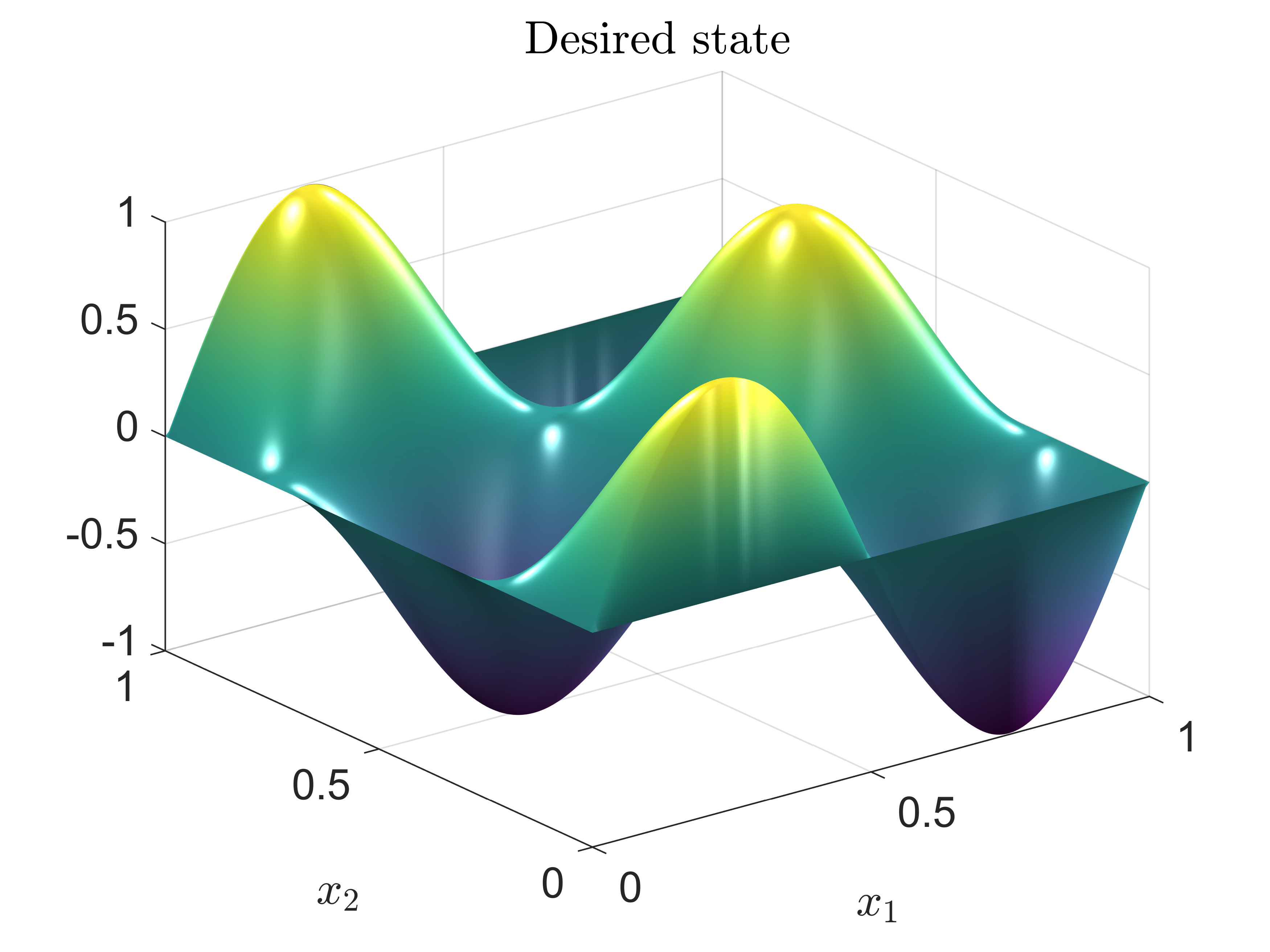
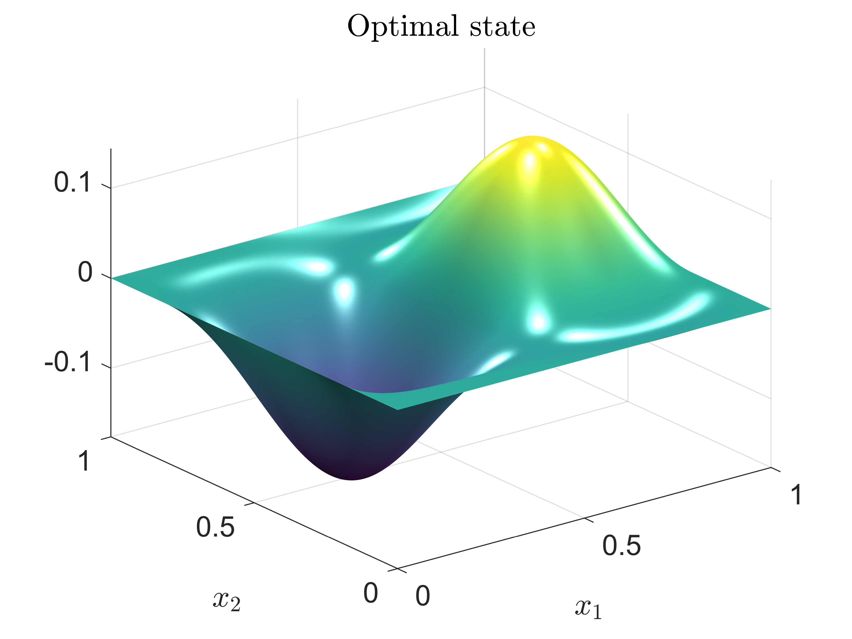
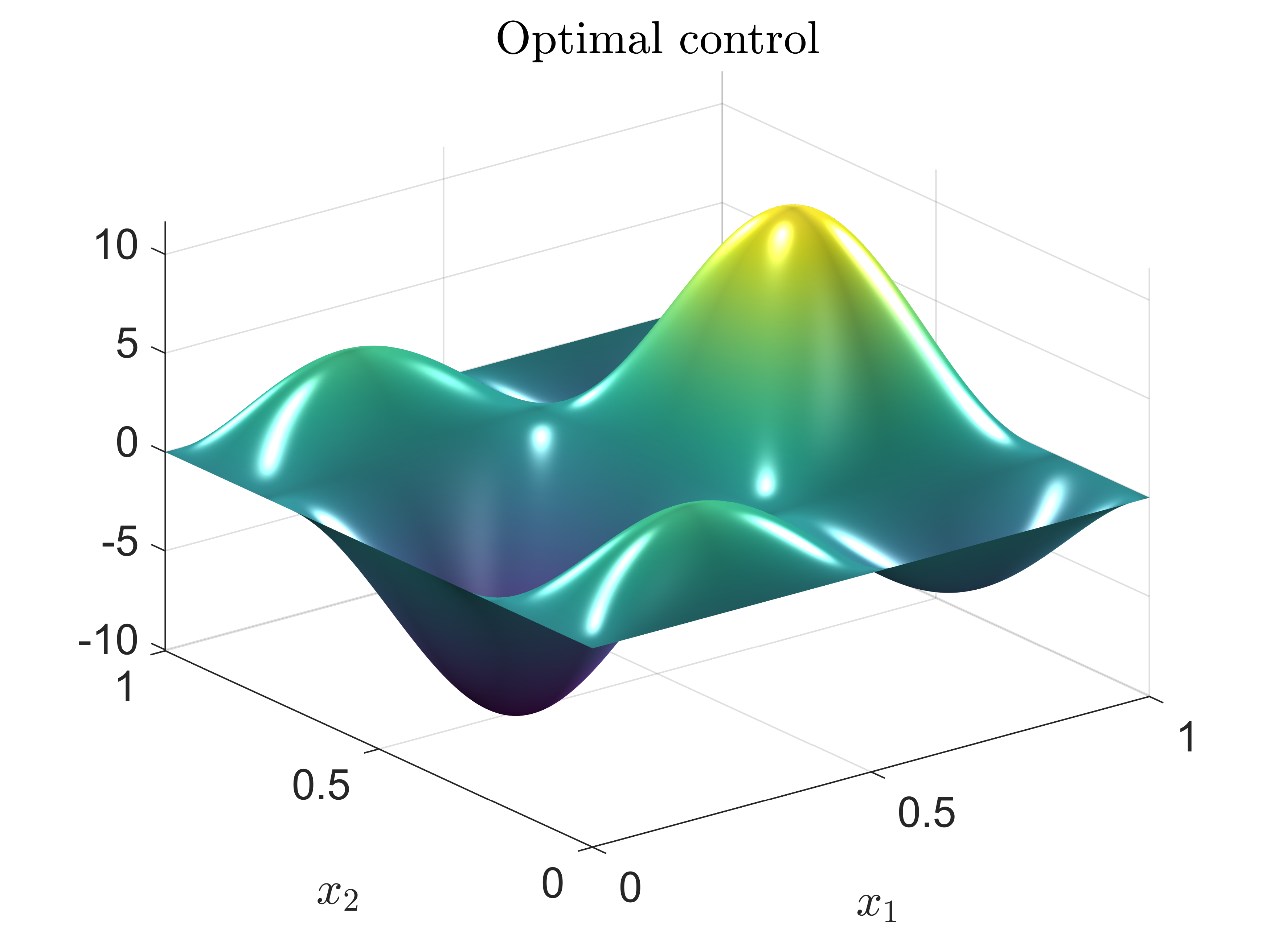
Figure 2: Desired state $y_{d}$, optimal state $\bar{y}=y_{\bar{u}}$, optimal control $\bar{u}$

		iter	$\#f$	$\#{\cal P}$	$\alpha=1$	$\alpha_{\max}$	$\alpha_{\min}$	$Q_{f}/Q_{f}^{3}$	$Q_{x}/Q_{x}^{3}$	$Q_{g}/Q_{g}^{3}$
Armijo	$(m=0)$	14	14	14	14	$1$	$1$	$0.997$/$0.07$	$0.9987$/$0.26$	$1.2$/$0.26$
Moré–Thuente	($m=0$)	14	17	14	13	$85$	$1$	$0.784$/$0.12$	$0.892$/$0.35$	$0.87$/$0.34$
Armijo	$(m=5)$	10	10	10	10	1	1	$0.997$/$0.03$	$0.9987$/$0.17$	$0.9985$/$0.19$
Moré–Thuente	($m=5$)	10	13	10	9	$85$	$1$	$0.784$/$0.03$	$0.892$/$0.17$	$0.87$/$0.18$
Armijo	$(m=10)$	8	8	8	8	1	$1$	$0.997$/$0.02$	$0.9987$/$0.16$	$0.9985$/$0.15$
Moré–Thuente	($m=10$)	8	11	8	7	85	$1$	$0.784$/$0.03$	$0.892$/$0.16$	$0.87$/$0.15$

Table 4: Results of 2 for Example 3, a nonconvex optimal control problem

Table 4 shows, for instance, that the full step is taken in all iterations for the Armijo line search and in all but one iteration for the Moré–Thuente line search. A closer inspection reveals that only the first iteration does not use a full step. We observe that although the problem is nonconvex, we have $y^{T}s>0$ in all iterations; cf. the values of $\#{\cal P}$ in Table 4. For $m=10$ we have $\text{iter}<m$, so any choice $m>10$ produces exactly the same results as for $m=10$. The values of $Q_{f}$, $Q_{x}$ and $Q_{g}$ indicate that for the Moré–Thuente line search we have q-linear convergence for the objective values, the iterates and also the gradients. Similar to Example 1, the last three columns of Table 4 hint at the fact that a significant acceleration takes place during the course of the algorithm.

An important property of efficient numerical algorithms for PDE-constrained optimization is their mesh independence, e.g. [ABPR86, KS87, HU04, AK22]. This roughly means that the number of iterations to reach a prescribed tolerance is insensitive to the mesh size. In Table 5 we examine this property for different values of $m$. The results clearly indicate mesh independence. In this example we used $\sigma=10^{-8}$ for the Moré–Thuente line search since $\sigma=10^{-4}$ sometimes failed.

	$\hat{M}=2^{j},j=$	$4$	$5$	$6$	$7$	$8$	$9$	$10$	$11$
Armijo	$(m=0)$	15	14	14	14	14	14	14	14
Moré–Thuente	($m=0$)	15	15	14	14	14	14	14	14
Armijo	$(m=5)$	10	10	10	10	10	10	10	10
Moré–Thuente	($m=5$)	10	10	10	10	10	10	10	10
Armijo	$(m=10)$	8	8	8	8	8	8	8	8
Moré–Thuente	($m=10$)	8	8	8	8	8	8	8	8

Table 5: Iteration numbers of 2 for Example 3 with different mesh sizes. The iteration numbers in each row are practically independent of the mesh size, which is reflective of the fact that the convergence results for 2 hold in $L^{2}(\Omega)$

6 Conclusion

This work introduces the first globally convergent modification of L-BFGS that recovers classical L-BFGS under sufficient optimality conditions. The method enjoys q-linear convergence for the objective values and $l$-step q-linear convergence for the iterates and the gradients for all sufficiently large $l$. The rates of convergence rely on strong convexity and gradient Lipschitz continuity, but only near one cluster point of the iterates; the existence of second derivatives is not required. The rates also hold for L-BFGS if the objective is strongly convex, improving the classical result [LN89, Theorem 7.1]. Numerical experiments support the theoretical findings and reveal that for sufficiently small parameter $c_{0}$, the new method and L-BFGS agree entirely. This may explain why L-BFGS is often successful for nonconvex problems.

Furthermore, this paper contains a proof of global convergence under the Wolfe–Powell conditions that requires only continuity of the gradient instead of Lipschitz continuity.

References

- [AB23] B. Azmi and M. Bernreuther. On the nonmonotone linesearch for a class of infinite-dimensional nonsmooth problems. arXiv preprint, 2023. doi:10.48550/arXiv.2303.01878.
- [ABGP14] M. Al-Baali, L. Grandinetti, and O. Pisacane. Damped techniques for the limited memory BFGS method for large-scale optimization. J. Optim. Theory Appl., 161(2):688–699, 2014. doi:10.1007/s10957-013-0448-8.
- [ABPR86] E. L. Allgower, K. Böhmer, F. A. Potra, and W. C. Rheinboldt. A mesh-independence principle for operator equations and their discretizations. SIAM J. Numer. Anal., 23(1):160–169, 1986. doi:10.1137/0723011.
- [ACG18] P. Ablin, J.-F. Cardoso, and A. Gramfort. Faster independent component analysis by preconditioning with hessian approximations. IEEE Trans. Signal Process., 66(15):4040–4049, 2018. doi:10.1109/TSP.2018.2844203.
- [AK20] B. Azmi and K. Kunisch. Analysis of the Barzilai-Borwein step-sizes for problems in Hilbert spaces. J. Optim. Theory Appl., 185(3):819–844, 2020. doi:10.1007/s10957-020-01677-y.
- [AK22] B. Azmi and K. Kunisch. On the convergence and mesh-independent property of the Barzilai-Borwein method for PDE-constrained optimization. IMA J. Numer. Anal., 42(4):2984–3021, 2022. doi:10.1093/imanum/drab056.
- [And21] N. Andrei. A new accelerated diagonal quasi-Newton updating method with scaled forward finite differences directional derivative for unconstrained optimization. Optimization, 70(2):345–360, 2021. doi:10.1080/02331934.2020.1712391.
- [BB88] J. Barzilai and J. M. Borwein. Two-point step size gradient methods. IMA J. Numer. Anal., 8(1):141–148, 1988. doi:10.1093/imanum/8.1.141.
- [BBEM19] J. Brust, O. Burdakov, J. B. Erway, and R. F. Marcia. A dense initialization for limited-memory quasi-Newton methods. Comput. Optim. Appl., 74(1):121–142, 2019. doi:10.1007/s10589-019-00112-x.
- [BDH19] O. Burdakov, Y. Dai, and N. Huang. Stabilized Barzilai-Borwein method. J. Comput. Math., 37(6):916–936, 2019. doi:10.4208/jcm.1911-m2019-0171.
- [BDLP21] J. J. Brust, Z. (W.) Di, S. Leyffer, and C. G. Petra. Compact representations of structured BFGS matrices. Comput. Optim. Appl., 80(1):55–88, 2021. doi:10.1007/s10589-021-00297-0.
- [BGZY17] O. Burdakov, L. Gong, S. Zikrin, and Y.-X. Yuan. On efficiently combining limited-memory and trust-region techniques. Math. Program. Comput., 9(1):101–134, 2017. doi:10.1007/s12532-016-0109-7.
- [BJRT22] A. S. Berahas, M. Jahani, P. Richtárik, and M. Takáč. Quasi-Newton methods for machine learning: forget the past, just sample. Optim. Methods Softw., 37(5):1668–1704, 2022. doi:10.1080/10556788.2021.1977806.
- [BMPS22] J. J. Brust, R. F. Marcia, C. G. Petra, and M. A. Saunders. Large-scale optimization with linear equality constraints using reduced compact representation. SIAM J. Sci. Comput., 44(1):a103–a127, 2022. doi:10.1137/21M1393819.
- [BN89] R. H. Byrd and J. Nocedal. A tool for the analysis of quasi-Newton methods with application to unconstrained minimization. SIAM J. Numer. Anal., 26(3):727–739, 1989. doi:10.1137/0726042.
- [BNS94] R. H. Byrd, J. Nocedal, and R. B. Schnabel. Representations of quasi-Newton matrices and their use in limited memory methods. Math. Program., 63(2 (A)):129–156, 1994. doi:10.1007/BF01582063.
- [CD18] S. Cipolla and F. Durastante. Fractional pde constrained optimization: An optimize-then-discretize approach with l-bfgs and approximate inverse preconditioning. Appl. Numer. Math., 123:43–57, 2018. doi:10.1016/j.apnum.2017.09.001.
- [CDLRT08] E. Casas, J. C. De Los Reyes, and F. Tröltzsch. Sufficient second-order optimality conditions for semilinear control problems with pointwise state constraints. SIAM J. Optim., 19(2):616–643, 2008. doi:10.1137/07068240X.
- [CPRZ23] S. Crisci, F. Porta, V. Ruggiero, and L. Zanni. Hybrid limited memory gradient projection methods for box-constrained optimization problems. Comput. Optim. Appl., 84(1):151–189, 2023. doi:10.1007/s10589-022-00409-4.
- [DABY15] Y.-H. Dai, M. Al-Baali, and X. Yang. A positive Barzilai-Borwein-like stepsize and an extension for symmetric linear systems. In Numerical analysis and optimization. Selected papers based on the presentations at the 3rd international conference, pages 59–75. Cham: Springer, 2015. doi:10.1007/978-3-319-17689-5_3.
- [Dai02] Y.-H. Dai. Convergence properties of the BFGS algoritm. SIAM J. Optim., 13(3):693–701, 2002. doi:10.1137/S1052623401383455.
- [Dai13a] Y.-H. Dai. A new analysis on the Barzilai-Borwein gradient method. J. Oper. Res. Soc. China, 1(2):187–198, 2013. doi:10.1007/s40305-013-0007-x.
- [Dai13b] Y.-H. Dai. A perfect example for the BFGS method. Math. Program., 138(1-2 (A)):501–530, 2013. doi:10.1007/s10107-012-0522-2.
- [DF05] Y.-H. Dai and R. Fletcher. Projected Barzilai-Borwein methods for large-scale box-constrained quadratic programming. Numer. Math., 100(1):21–47, 2005. doi:10.1007/s00211-004-0569-y.
- [DHL19] Y.-H. Dai, Y. Huang, and X.-W. Liu. A family of spectral gradient methods for optimization. Comput. Optim. Appl., 74(1):43–65, 2019. doi:10.1007/s10589-019-00107-8.
- [DHSZ06] Y. Dai, W. W. Hager, K. Schittkowski, and H. Zhang. The cyclic Barzilai-Borwein method for unconstrained optimization. IMA J. Numer. Anal., 26(3):604–627, 2006. doi:10.1093/imanum/drl006.
- [DKA] D. M. Dunlavy, T. G. Kolda, and E. Acar. Poblano toolbox for matlab v1.2. Accessed: 2023-03-25. URL: https://github.com/sandialabs/poblano_toolbox.
- [DKA10] D. M. Dunlavy, T. G. Kolda, and E. Acar. Poblano v1.0: A matlab toolbox for gradient-based optimization. Sandia Report SAND2010-1422, 2010. URL: https://www.osti.gov/servlets/purl/989350.
- [DKPS15] T. Dunst, M. Klein, A. Prohl, and A. Schäfer. Optimal control in evolutionary micromagnetism. IMA J. Numer. Anal., 35(3):1342–1380, 2015. doi:10.1093/imanum/dru034.
- [DL02] Y. Dai and L.-Z. Liao. -linear convergence of the Barzilai and Borwein gradient method. IMA J. Numer. Anal., 22(1):1–10, 2002. doi:10.1093/imanum/22.1.1.
- [DM19] A. Dener and T. Munson. Accelerating limited-memory quasi-newton convergence for large-scale optimization. In J. M. F. Rodrigues and P. J. S. et al. Cardoso, editors, Computational Science – ICCS 2019, pages 495–507, Cham, 2019. Springer International Publishing. doi:10.1007/978-3-030-22744-9_39.
- [DS96] J. E. jun. Dennis and R. B. Schnabel. Numerical methods for unconstrained optimization and nonlinear equations, volume 16 of Class. Appl. Math. Philadelphia, PA: SIAM, repr. edition, 1996. doi:10.1137/1.9781611971200.
- [FR21] L. Failer and T. Richter. A Newton multigrid framework for optimal control of fluid-structure interactions. Optim. Eng., 22(4):2009–2037, 2021. doi:10.1007/s11081-020-09498-8.
- [FVM22] L. Fang, S. Vandewalle, and J. Meyers. A parallel-in-time multiple shooting algorithm for large-scale pde-constrained optimal control problems. J. Comput. Phys., 452:110926, 2022. doi:10.1016/j.jcp.2021.110926.
- [GL89] J. C. Gilbert and C. Lemaréchal. Some numerical experiments with variable-storage quasi-Newton algorithms. Math. Program., 45(3 (B)):407–435, 1989. doi:10.1007/BF01589113.
- [GLL86] L. Grippo, F. Lampariello, and S. Lucidi. A nonmonotone line search technique for Newton’s method. SIAM J. Numer. Anal., 23:707–716, 1986. doi:10.1137/0723046.
- [GO23] J. Gao and Y. Ou. A hybrid BB-type method for solving large scale unconstrained optimization. J. Appl. Math. Comput., 69(2):2105–2133, 2023. doi:10.1007/s12190-022-01826-8.
- [Gri86] A. Griewank. Rates of convergence for secant methods on nonlinear problems in Hilbert space. In J.-P. Hennart, editor, Numerical Analysis, pages 138–157. Springer Berlin Heidelberg, 1986. doi:10.1007/BFb0072677.
- [Gri91] A. Griewank. The global convergence of partitioned BFGS on problems with convex decompositions and Lipschitzian gradients. Math. Program., 50(2 (A)):141–175, 1991. doi:10.1007/BF01594933.
- [GS81] W. A. Gruver and E. Sachs. Algorithmic methods in optimal control. Research Notes in Mathematics, 47. Boston, London, Melbourne: Pitman Advanced Publishing Program. X, 1981.
- [GS02] L. Grippo and M. Sciandrone. Nonmonotone globalization techniques for the Barzilai-Borwein gradient method. Comput. Optim. Appl., 23(2):143–169, 2002. doi:10.1023/A:1020587701058.
- [HD20] A. Hosseini Dehmiry. The global convergence of the BFGS method under a modified Yuan-Wei-Lu line search technique. Numer. Algorithms, 84(2):781–793, 2020. doi:10.1007/s11075-019-00779-7.
- [HU04] M. Hintermüller and M. Ulbrich. A mesh-independence result for semismooth Newton methods. Math. Program., 101(1 (B)):151–184, 2004. doi:10.1007/s10107-004-0540-9.
- [KD15] C. X. Kou and Y. H. Dai. A modified self-scaling memoryless Broyden-Fletcher-Goldfarb-Shanno method for unconstrained optimization. J. Optim. Theory Appl., 165(1):209–224, 2015. doi:10.1007/s10957-014-0528-4.
- [KS87] C. T. Kelley and E. W. Sachs. Quasi-newton methods and unconstrained optimal control problems. SIAM J. Control Optim., 25(6):1503–1516, 1987. doi:10.1137/0325083.
- [KS23] C. Kanzow and D. Steck. Regularization of limited memory quasi-Newton methods for large-scale nonconvex minimization. Math. Program. Comput., 15(3):417–444, 2023. doi:10.1007/s12532-023-00238-4.
- [Kup96] F.-S. Kupfer. An infinite-dimensional convergence theory for reduced SQP methods in Hilbert space. SIAM J. Optim., 6(1):126–163, 1996. doi:10.1137/0806008.
- [LBL02] D. R. Luke, J. V. Burke, and R. G. Lyon. Optical wavefront reconstruction: theory and numerical methods. SIAM Rev., 44(2):169–224, 2002. doi:10.1137/S003614450139075.
- [LF01a] D. Li and M. Fukushima. A modified BFGS method and its global convergence in nonconvex minimization. J. Comput. Appl. Math., 129(1-2):15–35, 2001. doi:10.1016/S0377-0427(00)00540-9.
- [LF01b] D.-H. Li and M. Fukushima. On the global convergence of the BFGS method for nonconvex unconstrained optimization problems. SIAM J. Optim., 11(4):1054–1064, 2001. doi:10.1137/S1052623499354242.
- [Liu14] T.-W. Liu. A regularized limited memory BFGS method for nonconvex unconstrained minimization. Numer. Algorithms, 65(2):305–323, 2014. doi:10.1007/s11075-013-9706-y.
- [LMP21] J. Lemoine, A. Münch, and P. Pedregal. Analysis of continuous -least-squares methods for the steady Navier-Stokes system. Appl. Math. Optim., 83(1):461–488, 2021. doi:10.1007/s00245-019-09554-5.
- [LN89] D. C. Liu and J. Nocedal. On the limited memory BFGS method for large scale optimization. Math. Program., 45(3 (B)):503–528, 1989. doi:10.1007/BF01589116.
- [LWH22] D. Li, X. Wang, and J. Huang. Diagonal BFGS updates and applications to the limited memory BFGS method. Comput. Optim. Appl., 81(3):829–856, 2022. doi:10.1007/s10589-022-00353-3.
- [MAM23] F. Mannel, H. O. Aggrawal, and J. Modersitzki. A structured L-BFGS method and its application to inverse problems. Inverse Probl. (status: minor revision required), arXiv preprint available, 2023. doi:10.48550/arXiv.2310.07296.
- [Mas04] W. F. Mascarenhas. The BFGS method with exact line searches fails for non-convex objective functions. Math. Program., 99(1 (A)):49–61, 2004. doi:10.1007/s10107-003-0421-7.
- [ML13] S. M. Marjugi and W. J. Leong. Diagonal Hessian approximation for limited memory quasi-Newton via variational principle. J. Appl. Math., 2013:8, 2013. Id/No 523476. doi:10.1155/2013/523476.
- [MQ80] R. V. Mayorga and V. H. Quintana. A family of variable metric methods in function space, without exact line searches. J. Optim. Theory Appl., 31:303–329, 1980. doi:10.1007/BF01262975.
- [MR21] F. Mannel and A. Rund. A hybrid semismooth quasi-Newton method for nonsmooth optimal control with PDEs. Optim. Eng., 22(4):2087–2125, 2021. doi:10.1007/s11081-020-09523-w.
- [MT94] J. J. Moré and D. J. Thuente. Line search algorithms with guaranteed sufficient decrease. ACM Trans. Math. Softw., 20(3):286–307, 1994. doi:10.1145/192115.192132.
- [Nes18] Y. Nesterov. Lectures on convex optimization, volume 137 of Springer Optim. Appl. Cham: Springer, 2nd edition edition, 2018. doi:10.1007/978-3-319-91578-4.
- [Noc80] J. Nocedal. Updating quasi-Newton matrices with limited storage. Math. Comput., 35:773–782, 1980. doi:10.2307/2006193.
- [NVM16] C. Nita, S. Vandewalle, and J. Meyers. On the efficiency of gradient based optimization algorithms for dns-based optimal control in a turbulent channel flow. Comput. Fluids, 125:11–24, 2016. doi:10.1016/j.compfluid.2015.10.019.
- [NW06] J. Nocedal and S. J. Wright. Numerical optimization. New York, NY: Springer, 2nd edition, 2006. doi:10.1007/978-0-387-40065-5.
- [Ore82] S. S. Oren. Perspectives on self-scaling variable metric algorithms. J. Optim. Theory Appl., 37:137–147, 1982. doi:10.1007/BF00934764.
- [Pow78] M. J. D. Powell. Algorithms for nonlinear constraints that use Lagrangian functions. Math. Program., 14:224–248, 1978. doi:10.1007/BF01588967.
- [Ray97] M. Raydan. The Barzilai and Borwein gradient method for the large scale unconstrained minimization problem. SIAM J. Optim., 7(1):26–33, 1997. doi:10.1137/S1052623494266365.
- [Sch16] F. Schöpfer. Linear convergence of descent methods for the unconstrained minimization of restricted strongly convex functions. SIAM J. Optim., 26(3):1883–1911, 2016. doi:10.1137/140992990.
- [TP15] D. A. Tarzanagh and M. R. Peyghami. A new regularized limited memory BFGS-type method based on modified secant conditions for unconstrained optimization problems. J. Glob. Optim., 63(4):709–728, 2015. doi:10.1007/s10898-015-0310-7.
- [TSY22] H. Tankaria, S. Sugimoto, and N. Yamashita. A regularized limited memory BFGS method for large-scale unconstrained optimization and its efficient implementations. Comput. Optim. Appl., 82(1):61–88, 2022. doi:10.1007/s10589-022-00351-5.
- [VPP20] R. G. Vuchkov, C. G. Petra, and N. Petra. On the derivation of quasi-Newton formulas for optimization in function spaces. Numer. Funct. Anal. Optim., 41(13):1564–1587, 2020. doi:10.1080/01630563.2020.1785496.
- [WHZ12] Z. Wan, S. Huang, and X. Zheng. New cautious BFGS algorithm based on modified Armijo-type line search. J. Inequal. Appl., 2012:10, 2012. Id/No 241. doi:10.1186/1029-242X-2012-241.
- [WLQ06] Z. Wei, G. Li, and L. Qi. New quasi-Newton methods for unconstrained optimization problems. Appl. Math. Comput., 175(2):1156–1188, 2006. doi:10.1016/j.amc.2005.08.027.
- [XLW13] Y.-H. Xiao, T.-F. Li, and Z.-X. Wei. Global convergence of a modified limited memory BFGS method for non-convex minimization. Acta Math. Appl. Sin., Engl. Ser., 29(3):555–566, 2013. doi:10.1007/s10255-013-0233-3.
- [Yan22] Y. Yang. A robust bfgs algorithm for unconstrained nonlinear optimization problems. Optimization, 0(0):1–23, 2022. doi:10.1080/02331934.2022.2124869.
- [YLL22] G. Yuan, P. Li, and J. Lu. The global convergence of the BFGS method with a modified WWP line search for nonconvex functions. Numer. Algorithms, 91(1):353–365, 2022. doi:10.1007/s11075-022-01265-3.
- [YWL17] G. Yuan, Z. Wei, and X. Lu. Global convergence of BFGS and PRP methods under a modified weak Wolfe-Powell line search. Appl. Math. Modelling, 47:811–825, 2017. doi:10.1016/j.apm.2017.02.008.
- [YWS20] G. Yuan, X. Wang, and Z. Sheng. The projection technique for two open problems of unconstrained optimization problems. J. Optim. Theory Appl., 186(2):590–619, 2020. doi:10.1007/s10957-020-01710-0.
- [YZZ22] G. Yuan, M. Zhang, and Y. Zhou. Adaptive scaling damped BFGS method without gradient Lipschitz continuity. Appl. Math. Lett., 124:7, 2022. Id/No 107634. doi:10.1016/j.aml.2021.107634.