Safe Chance-constrained Model Predictive Control under Gaussian Mixture Model Uncertainty

Abstract

We present a chance-constrained model predictive control (MPC) framework under Gaussian mixture model (GMM) uncertainty. Specifically, we consider the uncertainty that arises from predicting future behaviors of moving obstacles, which may exhibit multiple modes (for example, turning left or right). To address the multi-modal uncertainty distribution, we propose three MPC formulations: nominal chance-constrained planning, robust chance-constrained planning, and contingency planning. We prove that closed-loop trajectories generated by the three planners are safe. The approaches differ in conservativeness and performance guarantee. In particular, the robust chance-constrained planner is recursively feasible under certain assumptions on the propagation of prediction uncertainty. On the other hand, the contingency planner generates a less conservative closed-loop trajectory than the nominal planner. We validate our planners using state-of-the-art trajectory prediction algorithms in autonomous driving simulators.

I Introduction

Autonomous systems, such as self-driving cars and robots, face significant challenges when operating in dynamic environments. For instance, an autonomous vehicle must plan its trajectory while avoiding collisions with other road agents, such as other vehicles and pedestrians, with uncertain future positions. The future movements of other road agents are often multi-modal, for example, a nearby vehicle may go straight or turn at intersections. Planning safe trajectories in scenarios involving multi-modal behavior of road agents (e.g., intersection, overtaking) is particularly challenging yet essential for real-world applications. Our work here focuses on developing a provably safe and computationally tractable trajectory planning approach in the presence of multi-modal uncertainty distributions.

I-A Related Works

Risk-constrained trajectory planning is a common formulation to ensure safety in uncertain environments. This formulation, rather than enforcing constraints for all uncertainty realizations, tolerates constraint violation up to a given threshold in terms of a chosen risk metric. The chance constraint is a common risk metric that restricts the probability of constraint violation. However, the chance constraint formulation is unaware of the potential severity of constraint violation. This has motivated the use of conditional value-at-risk (CVaR) [1, 2, 3], which accounts for the expected amount of constraint violation. Both chance-constrained and CVaR-constrained trajectory planning problems are tractable when constraints are linear, and the uncertainty follows a (uni-modal) Gaussian distribution [4, 5, 6, 7].

In the context of autonomous driving, the trajectory prediction models [8, 9] show that in complex and interactive environments, the probability distributions over the future positions of the vehicles are multi-modal. These past works have used a Gaussian mixture model (GMM) to depict the multi-modal uncertainty. Motivated by the prevalence of GMM in trajectory predictions, our work focuses on developing a framework for safe trajectory planning under GMM uncertainty. When the moments of each mode of GMM uncertainty are known and constraints are linear, chance-constrained problems can be tractably solved [10], while CVaR-constrained problems can be addressed by an iterative cutting-plane [11] approach.

However, the exact distribution may be unknown in practice, and only samples (e.g., sensor data) may be available. Without any prior knowledge of the uncertainty’s distribution, CVaR-constrained problems have been tractably addressed by a sample average approximation [2] without any theoretical approximation guarantees. On the other hand, a distributionally robust approach with Wasserstein distance ambiguity set [12] can be applied to trajectory planning [13]. Under certain assumptions on the risk constraints, a finite-sample safety guarantee has been derived for this approach. With partial knowledge of the uncertainty’s distribution, e.g., the uncertainty is multi-modal and the number of modes is known, [14] extends the scenario approach [15, 16] to address trajectory planning under multi-modal uncertainty. On the other hand, [17] estimates the GMM moments by clustering the samples and robustifies the risk constraints against estimation error using moment concentration bounds. However, in the context of trajectory planning, both our prior studies [14, 17] are based on an open-loop framework.

In autonomous vehicle trajectory planning, overly cautious behavior or infeasibility issues are frequently observed in fast-changing and highly uncertain environments. Model Predictive Control (MPC) [18, 19, 20] address the problem by solving the trajectory planning problem in a receding-horizon manner. Leveraging the advancements in highly accurate sensors and real-time forecasting models, one can plan the ego vehicle’s (EV’s) trajectory with frequently updated observations and predictions in a closed-loop fashion. Past works on autonomous driving developed MPC under GMM uncertainty [21], showcasing its efficacy through simulations. However, no theoretical guarantees were provided.

One major obstacle hindering the safety of MPC is the recursive feasibility problem. It requires the existence of a feasible control input for each time step; the absence of such a solution indicates a potential violation of the safety constraints. This property has been well-studied in MPC under deterministic settings [22]. Among stochastic MPC frameworks, some previous works [23] make direct recursive feasibility assumptions. In contrast, when the uncertainty has bounded support, other research focuses on proving recursive feasibility [24] or identifying safe control invariant sets [25] where the system can deterministically remain feasible for an indefinite period of time. However, defining such sets becomes difficult for risk-constrained trajectory planning with unbounded GMM uncertainties.

I-B Contributions

We develop an MPC framework for autonomous driving under GMM uncertainty with a provable safety guarantee. Our main contributions are:

• Developing a recursively feasible and safe MPC framework. To this end, we develop conditions on the propagation of the GMM prediction over planning steps, and tighten the constraints of the MPC accordingly to robustify against the prediction propagation;

• Formulating an alternative planning scheme based on contingency planning [26], for reducing conservatism of chance-constrained MPC under GMM uncertainty while preserving the safety guarantees;

• Validating our methods by simulating with the state-of-the-art trajectory prediction model Trajectron++ [8] in an autonomous driving simulator CARLA [27].

The rest of the paper is organized as follows. In Section II, we formulate the chance-constrained MPC problems with GMM uncertain parameters and present a planning framework combining shrinking and receding horizon planning schemes. Section III presents an MPC scheme and develops the recursive feasibility and safety guarantees under assumptions on the GMM predictions. Furthermore, we present an alternative contingency planning scheme for reducing conservatism without losing the safety guarantee. Section IV demonstrates our methods on a state-of-the-art autonomous driving simulator.

Notation: A Gaussian distribution with mean $\mu$ and covariance matrix $\Sigma$ is denoted as $\mathcal{N}(\mu,\Sigma)$. By $\text{\textPsi}^{-1}(\cdot)$, we denote the inverse cumulative distribution function of the standard Gaussian distribution $\mathcal{N}(0,1)$. We denote a set of consecutive integers $\{a,a+1,\dots,b\}$ by $\mathbb{Z}_{a\mathrel{\mathop{\mathchar 58\relax}}b}$. We denote the conjunction by $\bigwedge$ and the disjunction by $\bigvee$. The weighted $L_{2}$ norm of a vector $x$ with a weighting matrix $P\succ 0$ is $\|x\|_{P}=\sqrt{x^{T}Px}$.

II Problem Formulation

Our goal is to find the optimal ego vehicle (EV) state trajectory that minimizes a specific cost function (e.g., fuel consumption or distance to the target) while ensuring a collision-free path in the presence of other vehicles (OVs) throughout the planning horizon. The EV is modeled as a deterministic linear time-varying system

$$x_{t+1}=A_{t}x_{t}+B_{t}u_{t},$$ (1)

where $x_{t}\in\mathbb{R}^{n_{x}}$ and $u_{t}\in\mathbb{R}^{n_{u}}$ denote the state and input at time $t$, and $A_{t}\in\mathbb{R}^{n_{x}\times n_{x}}$ and $B_{t}\in\mathbb{R}^{n_{x}\times n_{u}}$ are system’s dynamics matrices. To comply with road rules such as staying within lanes and adhering to speed limits, the state and control input are confined within time-invariant convex sets,

$$x_{t}\in\mathcal{X}\text{ and }u_{t}\in\mathcal{U}.$$ (2)

Given an initial state $x_{0}$ and a planning horizon $T$, the trajectory planning framework generates a sequence of control inputs $\textbf{u}=(u_{0},u_{1},\dots,u_{T-1})$. Given the initial state $x_{0}$ and the system dynamics (1), the input sequence u would lead to a state trajectory $\textbf{x}=(x_{0},x_{1},\dots,x_{T})$ that should be free from collisions with $J$ other vehicles (OVs) while satisfying the constraints (2). The $j$-th OV is modeled as a polytope with $I_{j}$ edges. For brevity, we use $\mathcal{X}_{t,j}^{safe}$ to denote the set of the EV states that lie outside of the polytope corresponding to the $j^{th}$ OV at time $t$. This collision avoidance set can be represented as the EV states that lie beyond at least one edge of the OV polytope. Hence, $\mathcal{X}_{t,j}^{safe}$ can be written as a disjunction of linear constraints: $x_{t}\in\mathcal{X}_{t,j}^{safe}\Leftrightarrow\bigvee_{i=1}^{I_{j}}\delta_{ij}^{t^{\intercal}}\tilde{x}_{t}\leq 0$, where $\tilde{x}_{t}=[x_{t}^{\intercal}\;\;1]^{\intercal}$ and the uncertainty $\delta_{ij}^{t}\in\mathbb{R}^{n_{x}+1}$ corresponds to the $i^{th}$ face of the $j^{th}$ OV at time $t$. A 2-dimensional space example, i.e., $n_{x}=2$, is shown in Fig. 1, where the EV states lying in the shaded orange region are considered to be free from collision with the OV.

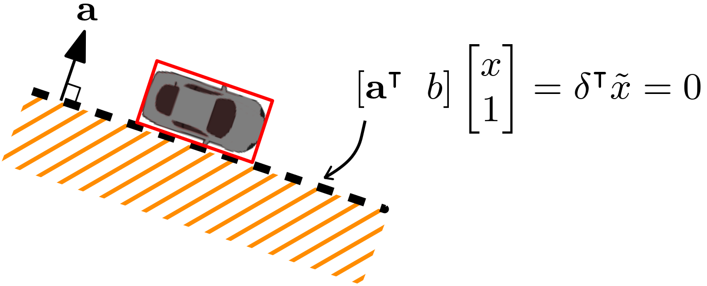
Figure 1: Polyhedral OV and linear constraint for collision avoidance in 2-dimensional space.

To capture the uncertain and multi-modal behavior of the OVs (e.g., an OV may go straight or turn at an intersection), we use a GMM to model the underlying distribution of the OV uncertainty $\delta_{ij}^{t}$ and enforce the following assumption.

Assumption 1.

[GMM uncertainty] The multi-modal uncertainty $\delta_{ij}^{t}$ is GMM distributed with $K_{j}$ modes of behavior, i.e., $\delta_{ij}^{t}\sim\sum_{k=1}^{K_{j}}\pi_{k}\cdot\mathcal{N}(\mu_{ijk}^{t},\Sigma_{ijk}^{t})$.

II-A Selection of Risk-constrained Formulation

TABLE I: Summary of risk-constrained approaches under GMM uncertainty

	Risk Measure	Method	Comp. time (s)	Risk constraint guarantee
Known GMM	Chance	(M1) Moment Trust Approach [10]	$2.60\times 10^{-1}$	100%
	CVaR	(M2) Iterative Cutting-plane [11]	$6.39\times 10^{0}$	None
Data-driven Case	Chance	(M3) Moment Robust Approach [17]	$2.47\times 10^{-1}$	Probabilistic
		(M4) Scenario Approach[14]	$4.28\times 10^{-5}$	Probabilistic
	CVaR	(M5) Sample Average Approximation [2]	$3.81\times 10^{0}$	None
		(M6) Distributionally Robust [12]	$3.00\times 10^{0}$	Probabilistic

To address the GMM uncertainty, we consider a risk-constrained formulation to ensure safety. To choose an appropriate risk metric and approach, we investigate six different risk-constrained methods. We evaluate the performances of the risk-constrained approaches based on a simple yet instructive example, consisting of a single risk-constrained optimization problem with a linear constraint function

$$\underset{x\in\mathbb{R}}{\text{min}} \;\;\;x,$$ (3a)

subject to $$\;\;\;\mathbb{P}(\delta\leq x)\geq 1-\epsilon,$$ (3b)

where $x\in\mathbb{R}$ is a decision variable and $\delta\in\mathbb{R}$ is a random variable with a GMM distribution $\delta\sim\sum_{k=1}^{K}\pi_{k}\cdot\mathcal{N}(\mu_{k},\Sigma_{k})$. For the risk metric, we consider either the original chance constraint (3b) (abbreviated as CC in this subsection) or a CVaR constraint, which is defined as

$${\text{CVaR}_{\epsilon}}\left(\delta-x\right)\mathrel{\mathop{\mathchar 58\relax}}=\inf_{\alpha>0}\left\{\frac{1}{\epsilon}\mathbb{E}[(\delta-x+\alpha)_{+}]-\alpha\right\}\leq 0.$$ (4)

The CVaR constraint (4) is a conservative approximation of the chance constraint (3b) [28]. For each of the two risk formulations (i.e., CC and CVaR), we apply existing tractable approaches based on the assumptions on the uncertainty’s distribution. In particular, we explore cases where the distribution is fully known, partially known, or completely unknown.

First, we consider the case when the exact GMM moments are known. The following risk-constrained methods can be employed to address uncertainty.

1. CC-Moment trust approach (MTA) [10]: When the exact GMM moments are known, the chance constraint (3b) can be equivalently formulated as the following constraints.

   $$\begin{cases}\Psi^{-1}(1-\epsilon_{k}){\sigma}_{k}+{\mu}_{k}\leq x,\;\;\forall k\\ \sum_{k}\pi_{k}\cdot\epsilon_{k}=\epsilon.\end{cases}$$

2. CVaR-MTA [11]: When the exact GMM moments are known, an iterative cutting plane algorithm [11] is designed to converge to a solution $x^{*}$ that satisfies (4).

Second, we consider the situations where $\delta$ is known to follow a GMM with $K$ modes, but the precise GMM moments are unknown, and only $N_{s}$ independent and identically distributed (i.i.d.) samples of $\delta$ are accessible from the true GMM distribution, denoted as $\delta^{(1)},\ldots,\delta^{(N_{s})}$. Given the number of modes, we can also determine mode $k$ where each sample belongs based on clustering methods [29]. We use $\delta_{k}^{(n)}$ to denote a sample number $n$ that belongs to mode $k$. In this case, the following methods can be applied to manage risk under uncertainty.

1. CC-Moment robust approach (MRA) [17]: The moments of the $k^{th}$ GMM mode can be estimated from the samples. MRA robustifies the estimated moments $(\hat{\mu}_{k},\hat{\sigma}_{k})$ and formulates

   $$\begin{cases}\Psi^{-1}(1-\epsilon_{k})\hat{\sigma}_{k}\sqrt{1+r_{2,k}}+\hat{\mu}_{k}+r_{1,k}\leq x,\;\;\forall k\\ \sum_{k}\pi_{k}\cdot\epsilon_{k}=\epsilon,\end{cases}$$

   where $r_{1,k}$ and $r_{2,k}$ quantifies the error bounds between the estimate and actual moments (see [17]). This approach provides a guarantee of the satisfaction of the chance constraint (3b) with $1-2\beta$ probability, where $\beta$ is a prescribed tolerance.

2. CC-scenario approach [14]: With the prior information on the number of modes and the mode $k$ where each sample belongs, the scenario approach formulates

   $$x\geq\max_{i}\left(\delta_{k}^{(i)}\right),\;\;\;\forall k.$$

   The solution of this constraint is guaranteed to satisfy the chance constraint (3b) with at least $1-\beta$ probability, where $\beta$ is determined by the prediction sample size $N_{s}$ and chance constraint risk bound $\epsilon$.

Third, we consider the case when there is no prior information on the distribution of $\delta$ and only $N_{s}$ i.i.d. samples of $\delta$ drawn from the true distribution are available. In this case, the following CVaR-constrained approaches can be employed.

1. CVaR-sample average approximation (SAA) method [2]: With $N_{s}$ samples of $\delta$, the SAA method estimates the CVaR constraint as

   $$\frac{1}{\epsilon N_{s}}\sum_{i=1}^{N_{s}}[(\delta^{(i)}-x+\alpha)_{+}]-\alpha\leq 0.$$

2. CVaR-distributionally robust (DR) approach [12] with Wasserstein-distance ambiguity set: The Wasserstein-distance DR CVaR constraint is formulated as

   $$\underset{Q\in\mathcal{Q}_{\gamma}(\hat{P}_{N_{s}})}{\text{sup}}\text{CVaR}_{\epsilon}^{Q}(\delta-x)\leq 0,$$

   where $\hat{P}_{N_{s}}$ is an empirical distribution of $\delta$ estimated with $N_{s}$ samples of $\delta$. Also, $\mathcal{Q}_{\gamma}(\hat{P}_{N_{s}})$ is the set of distributions whose Wasserstein distance from $\hat{P}_{N_{s}}$ is less than or equal to $\gamma$. This approach provides a satisfaction guarantee of the chance constraint (3b) with at least $1-\beta$ probability, where $\beta$ depends on the Wasserstein radius $\gamma$, sample size $N_{s}$ and the underlying distribution of $\delta$.

To compare the optimality, safety and computation time, we evaluate the above-mentioned risk-constrained methods on problem (3), subject to uncertainty with a bi-modal Gaussian distribution $\delta\sim 0.5\mathcal{N}(1,1)+0.5\mathcal{N}(10,1)$.

We use the approaches (M1)-(M6) to solve the above risk-constrained problem for 100 times. At each time, we draw $N_{s}=2000$ i.i.d. samples of $\delta$ from the GMM, and we cluster the samples into two modes and estimate the GMM moments $\{(\hat{\mu}_{k},\hat{\sigma}_{k})\}_{k=1}^{2}$. When the GMM moments are assumed to be known, particularly for methods (M1) and (M2), we trust the sample-estimated GMM moments. For (M3), we robustify against the moment estimation error. For methods (M4), (M5) and (M6), we directly use the samples to solve the risk-constrained problem. In each simulation, we obtain the optimal solutions $x^{*}$ based on the above-mentioned methods. After obtaining the optimal solution $x^{*}$, we evaluate the constraint violation probability based on the $10^{4}$ new test samples of $\delta$ drawn from the true distribution, i.e., we count the rate of $\delta^{n}_{\text{test}}\geq x^{*}$ among the new test samples $n=1,\ldots,10^{4}$.

We set the risk tolerance to be $\epsilon=0.05$. In methods (M1) and (M3), where we need to assign the risk to different GMM modes, we uniformly assign $\epsilon_{k}=\epsilon$ for all $k\in\mathbb{Z}_{1\mathrel{\mathop{\mathchar 58\relax}}K}$. For the CVaR-DR method (M6), we choose a Wasserstein radius of the ambiguity set to be $\gamma=0.04$.

Note that problem (3) aims at minimizing $x$, and a larger solution is safer to the risk constraint, as $\mathbb{P}(\delta\leq x)$ increases with the value of $x$. Hence, “less conservative” and “smaller optimal cost” will interchangeably describe a smaller solution of $x$.

The optimal solutions generated by different risk-constrained approaches and the empirical constraint violation probability over the 100 simulations are shown on the left and the right of Figure 2, respectively. Based on the results, (M1) and (M3), which rely on the assumption that the uncertainty conforms to GMM, achieve small optimal costs yet have a large but feasible (i.e., less than or equal to $\epsilon=5\%$) constraint violation probability. CVaR-constrained methods (M2) and (M5) yield more conservative solutions with a reduced probability of constraint violation. The CC-scenario method (M4) yields solutions that lead to a slightly higher cost than the CVaR-constrained framework. The CVaR-DR approach (M6) generates much more conservative results than the other methods with a zero constraint violation probability.

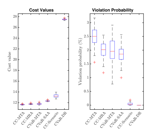
Figure 2: Optimality (left) and constraint violation (right) performances of the risk-constrained optimization methods.

The average computational time of the different risk-constrained methods over the 100 simulations is provided in the “Comp. time” column of Table I. The CVaR-constrained methods (M2) and (M5) significantly prolong the computation time. The CVaR-DR approach (M6) in general takes longer than chance-constrained methods, whereas the CC-scenario method (M4) has the lowest computational time among all risk-constrained approaches. This trend is consistent with the observations when using these risk-constrained methods in open-loop trajectory planning problems.

The key insight from this simple numerical study is that for the multi-modal uncertainty, the methods (M1) and (M3), which employ CC as a risk metric and incorporate distribution information, tend to yield less conservative solutions while ensuring computational efficiency. In contrast, enforcing CVaR constraints or distributional robustness may lead to an excessively conservative solution and significantly extend computation time. The safety constraint in autonomous car trajectory planning problems can be defined as a conjunction of single risk constraints for tractability [30, 2, 31], and we expect that the performances of the risk-constrained methods discussed in this subsection for a single risk constraint can be extended to such trajectory planning problems. To ensure that our trajectory planning framework is not overly conservative and to consider real-time planning for autonomous driving, we focus on the chance-constrained formulation in this work. Furthermore, to ensure recursive feasibility in MPC, we investigate the propagation of the distribution model (i.e., GMM) over planning steps. Therefore, we adopt CC-MTA (M1) and CC-MRA (M3) approaches to handle the chance constraints.

II-B Chance-constrained Planning

Recall the definition of the safe set of EV states, denoted as $\mathcal{X}_{t,j}^{safe}$; it represents the set of EV states that are free from collision with the $j^{th}$ OV at time $t$. To capture the collision avoidance in trajectory planning with $J$ OVs over a planning horizon $T$, we formulate a joint chance constraint

$$\mathbb{P}\left(\bigwedge_{t=1}^{T}\bigwedge_{j=1}^{J}x_{t}\in\mathcal{X}_{t,j}^{safe}\right)\geq 1-\epsilon.$$ (6)

The joint chance constraints can be transformed into tractable deterministic constraints. In particular, we first use the Big-M method [32] to handle the non-convexity of the disjunctive collision avoidance constraint (as illustrated in Fig. 1): $x_{t}\in\mathcal{X}_{t,j}^{safe}\Leftrightarrow\bigvee_{i=1}^{I_{j}}\delta_{ij}^{t^{\intercal}}\tilde{x}_{t}\leq 0\Leftrightarrow\bigwedge_{i=1}^{I_{j}}\delta_{ij}^{t^{\intercal}}\tilde{x}_{t}\leq Mz_{ij}^{t}$, where $M$ is a positive number that is larger than any possible value of the linear constraint and $z_{ij}^{t}\in\{0,1\}$ is a binary variable. Then, we use Boole’s inequality [33] to decouple the joint chance constraint into multiple single chance constraints. Based on Assumption 1, $\delta_{ij}^{t}$ conforms to a GMM. Given the moments $\mu_{ijk}^{t}$ and $\Sigma_{ijk}^{t}$, either known or estimated from samples, the single chance constraints can then be equivalently reformulated into second-order conic constraints. The resulting constraints are as follows.

$$\bigwedge_{t=1}^{T}\bigwedge_{j=1}^{J}\bigwedge_{i=1}^{I_{j}}\bigwedge_{k=1}^{K_{j}}\Gamma_{ijk}^{t}\sqrt{\tilde{x}_{t}^{\intercal}{\Sigma_{ijk}^{t}}\tilde{x}_{t}}+\tilde{x}_{t}^{\intercal}\mu_{ijk}^{t}\leq Mz_{ijk}^{t},$$ (7a)

$$\sum_{k=1}^{K_{j}}\pi_{k}\epsilon_{ijk}^{t}=\epsilon_{ij}^{t}=\epsilon/(TJ).$$ (7b)

$$\sum_{i=1}^{I_{j}}z_{ijk}^{t}=1,\;z_{ijk}^{t}\in\{0,1\},$$ (7c)

where $\Gamma_{ijk}^{t}\mathrel{\mathop{\mathchar 58\relax}}=\text{\textPsi}^{-1}(1-\epsilon_{ijk}^{t})$. Note that the reformulation is conservative (i.e., $\eqref{eq:chanceGMM}\Rightarrow\eqref{eq:MPCchance}$) due to the uniform allocation of $\epsilon$ to all OVs and timesteps [30, Lemma 1].

Previous work [14, 17] used an open-loop trajectory planning approach, which only supports a short planning horizon. In particular, when the planning horizon $T$ increases, the OV prediction becomes highly uncertain such that no feasible solution exists. For instance, our previous experimental results showed that using the Trajectron++ model [8] on real-world intersection data to forecast a vehicle’s position 4 seconds ahead results in a substantial state variation of up to 28 meters, posing a significant challenge to planning feasible trajectories for an EV. To address the infeasibility issues of open-loop planning over a long planning horizon, [21] proposed an MPC framework under GMM uncertainty. However, the issues of recursive feasibility and safety guarantees were not addressed.

To this end, our goal is to develop an MPC framework under GMM uncertainty with provable recursive feasibility and safety guarantees. In the rest of the paper, we use $\tau$ to denote the MPC planning steps and $T_{OH}$ to denote the open-loop planning horizon at each planning step. At each $\tau\in\{0,1,\ldots,T-1\}$, we update the GMM moment predictions: $(\mu_{ijk}^{t|\tau},\Sigma_{ijk}^{t|\tau})$ for future time steps $t=\tau+1,\tau+2,\ldots,T_{OH}$ based on the prediction module or sample estimation. Utilizing the predictions, we iteratively solve an open-loop trajectory planning problem up to $T_{OH}$.

We consider two common MPC planning horizon settings, as shown in Figure 3.

• Shrinking-horizon: $T_{OH}=T$, where we compute trajectories up to the end of the closed-loop planning horizon at each planning step $\tau$.

• Receding-horizon: $T_{OH}=\tau+T_{s}$, where we plan a trajectory for the upcoming $T_{s}$ timesteps ($T_{s}<T$) at each planning step.

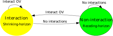
Figure 3: High-level state machine for MPC combining the shrinking-horizon and receding-horizon settings.

The shrinking-horizon setting is employed when the EV needs to complete a maneuver, such as a turn or a lane merge, within a finite time window and in the presence of OVs. Receding-horizon planning allows a longer closed-loop planning horizon and is used in non-interactive scenarios, such as lane keeping and car following. The transition from a non-interaction state to an interaction state occurs when the EV has a fixed-horizon goal in the presence of OVs. The occurrence of the state transition can be determined by the sensor observations. Since the OV-involved scenarios present the most challenge regarding uncertainties in future trajectories of OVs, our focus will be on deriving an MPC algorithm with provable recursive feasibility and safety in the shrinking-horizon setting.

III Chance-constrained MPC

At every MPC planning step $\tau=0,1,\ldots,T-1$, we solve a trajectory planning problem $\mathcal{P}$, to be specified in the following sections. The solution to the planning problem is the control input $\textbf{u}_{\tau}=(u_{\tau|\tau},u_{\tau+1|\tau},\dots,u_{T_{OH}-1|\tau})$ and open-loop state trajectory $\textbf{x}_{\tau}=(x_{\tau+1|\tau},x_{\tau+2|\tau},\dots,x_{T_{OH}|\tau})$. We actuate the EV with the first control input $u_{\tau|\tau}$ and proceed to the next time step. The algorithm that implements MPC over a closed-loop planning horizon $T$ is outlined in the pseudocode below.

Algorithm 1 Chance-constrained MPC

1:Initialize: initial state $x_{0}$, $\tau=0$, $T_{OH}$, problem $\mathcal{P}$

2:for $\tau=0,1,2,\ldots,T-1$ do

3:     Obtain GMM prediction: $(\mu^{t|\tau},\Sigma^{t|\tau}),\;\forall t\in\mathbb{Z}_{\tau+1\mathrel{\mathop{\mathchar 58\relax}}T_{OH}}$

4:     Solve $\mathcal{P}$

5:     if feasible then

6:         Obtain: $\textbf{u}_{\tau}$, $\textbf{x}_{\tau}$

7:         Actuate EV with $u_{\tau|\tau}$, reach $x_{\tau+1|\tau}$

8:     else

9:         return Infeasible      

10:return $\textbf{x}=\left(x_{(1|0)},x_{(2|1)},x_{(3|2)},\ldots,x_{(T|T-1)}\right)$

In the following, we present three approaches to formulating $\mathcal{P}$ in Algorithm 1. In subsection III-A, we present a nominal planner, which is a naive deterministic reformulation of chance-constrained MPC under GMM. In subsection III-B, we develop a robust MPC planner that implements tightened chance constraints and is proved to be recursively feasible under certain assumptions on the propagation of the GMM predictions across planning steps. Inspired by [26], in subsection III-C, we apply the concept of contingency planning to reduce the conservativeness of the chance-constrained MPC under GMM uncertainty.

III-A Nominal Planning

Our first approach to formulating $\mathcal{P}$ in Algorithm 1 is based on the deterministic formulation of the chance constraints as introduced in (7a).

$$\underset{\textbf{u}_{\tau},\;\textbf{z}_{\tau}}{\text{min}} \mathcal{J}(\textbf{u}_{\tau},\textbf{x}_{\tau})$$ (8a)

s.t. $$x_{t+1}=A_{t}x_{t}+B_{t}u_{t},\;\;\;\forall t\in\mathbb{Z}_{\tau\mathrel{\mathop{\mathchar 58\relax}}(T_{OH}-1)},$$ (8b)

$$\Gamma^{t}\sqrt{\tilde{x}_{t|\tau}^{\intercal}{\Sigma^{t|\tau}}\tilde{x}_{t|\tau}}+\tilde{x}_{t|\tau}^{\intercal}\mu^{t|\tau}\leq Mz^{t|\tau},$$

$$\;\;\;\;\;\;\;\;\;\;\;\;\;\;\;\;\;\;\;\;\;\;\;\;\;\;\;\;\;\;\;\;\;\;\;\;\;\;\;\;\forall t\in\mathbb{Z}_{(\tau+1)\mathrel{\mathop{\mathchar 58\relax}}T_{OH}},$$ (8c)

$$\eqref{eq:xuconstraints},\eqref{constraint:RAtj},\eqref{constraint:RAandBinary}.$$

Note that in (8c) and for the rest of this section, for brevity, we have excluded the sub-indices corresponding to OV $j$, mode number $k$, and the OV faces $i$ (see (7a)). In particular, constraint (8c) must be satisfied for all $j\in\mathbb{Z}_{1\mathrel{\mathop{\mathchar 58\relax}}J},\;k\in\mathbb{Z}_{1\mathrel{\mathop{\mathchar 58\relax}}K_{j}},\;i\in\mathbb{Z}_{1\mathrel{\mathop{\mathchar 58\relax}}I_{j}}$.

A major challenge in MPC is to ensure recursive feasibility (i.e., Algorithm 1 does not go to line 9). In the receding horizon case (as discussed in Section II-B), we consider non-interactive scenarios. In these scenarios, the constraints related to the OVs might be nonexistent, for example in a lane-keeping scenario where (8c) does not exist. In such cases, Algorithm 1 is recursively feasible when the terminal state $x_{T}$ lies in a terminal set that is control invariant for the EV system (1)-(2) [34, Thereom 12.1]. Alternatively, the uncertainty is minimal and admits a bounded support, for example when the EV follows a front car with constant speed. In such cases, the recursive feasibility can be ensured using the robust MPC methods that consider the robust constraint tightening against the worst-case uncertainty realization [35, 24]. In our MPC framework, we employ receding-horizon MPC when there exists no OV-related uncertainty. We assume that a control invariant terminal state set exists and thus the receding-horizon MPC is recursively feasible.

In autonomous driving scenarios where the OV states are highly uncertain, we employ shrinking-horizon planning. In the following subsection, we explore conditions on the growth of the GMM uncertainty along the planning steps and robustification of chance constraints against the worst-case uncertainty propagation, under which we can ensure the recursive feasibility of shrinking-horizon MPC.

III-B Robust Planning for Recursive Feasibility

During interactions between the EV and the OVs, our empirical findings from the forecasting model show the rather intuitive fact that prediction uncertainty reduces over time with updated observations of an OV. Moreover, the OV’s multi-modal behavior, such as the possibility of going straight or turning at intersections, gets reduced to one mode with ongoing observation over time. These observations motivate the following assumptions about the shrinkage of the OV prediction uncertainty in interactive scenarios. These assumptions are, in turn, used to ensure the recursive feasibility of a shrinking-horizon MPC problem.

Assumption 2.

The number of the prediction modes does not increase with planning steps, that is, $K^{\tau}\geq K^{\tau+1}$.

To quantify the difference in the prediction at time $\tau$ and $\tau+1$ of the OV position at time $t$, we investigate the propagation of the predicted GMM moments corresponding to each face of each OV under each mode of behavior. Let us define the Frobenius norm of the uncertainty’s covariance matrix between two consecutive time steps as

$$\sqrt{\mathinner{\!\left\lVert\Sigma^{t|\tau}\right\rVert}_{F}}-\sqrt{\mathinner{\!\left\lVert\Sigma^{t|\tau+1}\right\rVert}_{F}}=g^{t}(\tau).$$ (9)

The shift of the mean prediction between two consecutive time steps is denoted by

$$\mathinner{\!\left\lVert\mu^{t|\tau}-\mu^{t|\tau+1}\right\rVert}_{2}=h^{t}(\tau).$$ (10)

Assumption 3.

For any $t\in\mathbb{Z}_{2\mathrel{\mathop{\mathchar 58\relax}}T}$ and planning steps $\tau\in\mathbb{Z}_{0\mathrel{\mathop{\mathchar 58\relax}}t-1}$, the shift of the mean prediction is bounded by the covariance shift as follows:

$$h^{t}(\tau)\leq\Gamma^{t}\cdot g^{t}(\tau),$$ (11)

where $\Gamma^{t}=\text{\textPsi}^{-1}(1-\epsilon^{t})$ is the $(1-\epsilon^{t})$ quantile of the standard Gaussian distribution.

To ensure recursive feasibility, we introduce the following robust planning scheme $\mathcal{P}$ in Algorithm 1.

$$\underset{\textbf{u}_{\tau},\;\textbf{z}_{\tau}}{\text{min}} \mathcal{J}(\textbf{u}_{\tau},\textbf{x}_{\tau})$$ (12a)

s.t. $$\Gamma^{t}\sqrt{\mathinner{\!\left\lVert\Sigma^{t|\tau}\right\rVert}_{F}}\cdot\mathinner{\!\left\lVert\tilde{x}_{t|\tau}\right\rVert}_{2}+\tilde{x}_{t|\tau}^{\intercal}{\mu^{t|\tau}}\leq Mz^{t|\tau},$$

$$\;\;\;\;\;\;\;\;\;\;\;\;\;\;\;\;\;\;\;\;\;\;\;\;\;\;\;\;\;\;\;\;\;\;\;\;\;\;\;\;\;\;\;\;\forall t\in\mathbb{Z}_{(\tau+1)\mathrel{\mathop{\mathchar 58\relax}}T_{OH}},$$ (12b)

$$\eqref{eq:xuconstraints},\eqref{CL:dynamics},\eqref{constraint:RAtj},\eqref{constraint:RAandBinary}.$$ (12c)

Note that a feasible solution of (12) is also a feasible solution of (8), because (12b) is a conservative approximation of (8c) based on Cauchy–Schwarz inequality,

$$\sqrt{\tilde{x}_{t|\tau}^{\intercal}{\Sigma^{t|\tau}}\tilde{x}_{t|\tau}}\leq\sqrt{\mathinner{\!\left\lVert\Sigma^{t|\tau}\right\rVert}_{F}}\cdot\mathinner{\!\left\lVert\tilde{x}_{t|\tau}\right\rVert}_{2}.$$ (13)

Proposition 1.

[Shrinking-horizon recursive feasibility] Under Assumptions 1–3, the existence of a feasible solution for $\eqref{problem:RobustMPC}$ at $\tau=0$ ensures that Algorithm 1 with $\mathcal{P}$ set to (12) is recursively feasible.

Proof.

Suppose at some MPC planning step $\tau$, there exists a feasible solution of (12), where the state trajectory is $\textbf{x}_{\tau}=(x_{\tau+1|\tau},\dots,x_{T|\tau})$. At the next MPC planning step $\tau+1$, for any $t\in\mathbb{Z}_{(\tau+2)\mathrel{\mathop{\mathchar 58\relax}}T},$

$$\begin{split}&\;\Gamma^{t}\sqrt{\mathinner{\!\left\lVert\Sigma^{t|\tau+1}\right\rVert}_{F}}\cdot\mathinner{\!\left\lVert\tilde{x}_{t|\tau+1}\right\rVert}_{2}+\tilde{x}_{t|\tau+1}^{\intercal}{\mu^{t|\tau+1}}\\ \leq&\;\Gamma^{t}\sqrt{\mathinner{\!\left\lVert\Sigma^{t|\tau}\right\rVert}_{F}}\cdot\mathinner{\!\left\lVert\tilde{x}_{t|\tau+1}\right\rVert}_{2}+\tilde{x}_{t|\tau+1}^{\intercal}{\mu^{t|\tau}}\\ &\;\;\;\;+\biggl{(}h^{t}(\tau)-\Gamma^{t}\cdot g^{t}(\tau)\biggr{)}\cdot\mathinner{\!\left\lVert\tilde{x}_{t|\tau+1}\right\rVert}_{2}\\ \leq&\;\Gamma^{t}\sqrt{\mathinner{\!\left\lVert\Sigma^{t|\tau}\right\rVert}_{F}}\cdot\mathinner{\!\left\lVert\tilde{x}_{t|\tau+1}\right\rVert}_{2}+\tilde{x}_{t|\tau+1}^{\intercal}{\mu^{t|\tau}}.\end{split}$$ (14)

The first inequality is due to (9) and because from Cauchy-Schwarz inequality,

$$\tilde{x}_{t|\tau+1}^{\intercal}\left({\mu^{t|\tau+1}}-{\mu^{t|\tau}}\right) \leq\mathinner{\!\left\lVert\tilde{x}_{t|\tau+1}\right\rVert}_{2}\cdot\mathinner{\!\left\lVert\mu^{t|\tau+1}-{\mu^{t|\tau}}\right\rVert}_{2}$$

and therefore, by (10),

$$\tilde{x}_{t|\tau+1}^{\intercal}{\mu^{t|\tau+1}}\leq\tilde{x}_{t|\tau+1}^{\intercal}{\mu^{t|\tau}}+\mathinner{\!\left\lVert\tilde{x}_{t|\tau+1}\right\rVert}_{2}h^{t}(\tau).$$

The second inequality in (LABEL:proof:unifiedRF) follows from (11). If we set a state trajectory at $\tau+1$ to be $(x_{\tau+2|\tau+1},\ldots,x_{T|\tau+1})=(x_{\tau+2|\tau},\ldots,x_{T|\tau})$, then it satisfies

$$\Gamma^{t}\sqrt{\mathinner{\!\left\lVert\Sigma^{t|\tau+1}\right\rVert}_{F}}\cdot\mathinner{\!\left\lVert\tilde{x}_{t|\tau+1}\right\rVert}_{2}+\tilde{x}_{t|\tau+1}^{\intercal}{\mu^{t|\tau+1}}\leq Mz^{t|\tau}$$

by (LABEL:proof:unifiedRF). Note that $\Gamma^{t}$ remains the same throughout the proof. This is because $\Gamma^{t}$ depends only on $\epsilon^{t}$, which is the same for each mode $k$ and does not vary at different planning steps due to the uniform risk allocation (7b). Therefore, Algorithm 1 with $\mathcal{P}$ set to (12) is recursively feasible. ∎

Our next result shows that the planned trajectory satisfies the original chance constraint (6) over the closed-loop horizon $T$.

Theorem 1.

[Safety guarantee of MPC]

1. Under Assumption 1, if Algorithm 1 with $\mathcal{P}$ set to (8) does not return Infeasible and generates a closed-loop state trajectory x, then x satisfies the original chance constraint (6).

2. Under Assumptions 1–3, Algorithm 1 with $\mathcal{P}$ set to (12) never returns Infeasible and generates a closed-loop trajectory x if (12) is feasible with the initial state $x_{0}$. Moreover, x satisfies the original chance constraint (6).

Proof.

1) If Algorithm 1 with $\mathcal{P}$ set to (8) generates a closed-loop state trajectory $\textbf{x}=(x_{(1|0)},\ldots,x_{(T|T-1)})$, then $x_{t|t-1}$ satisfies (8c) for all $t\in\mathbb{Z}_{1\mathrel{\mathop{\mathchar 58\relax}}T}$. Considering every face across all modes of all OVs: $j\in\mathbb{Z}_{1\mathrel{\mathop{\mathchar 58\relax}}J},\;k\in\mathbb{Z}_{1\mathrel{\mathop{\mathchar 58\relax}}K_{j}},\;i\in\mathbb{Z}_{1\mathrel{\mathop{\mathchar 58\relax}}I_{j}}$, the closed-loop trajectory x also satisfies the conjunction of deterministic constraints (7a). Given the implication of $\eqref{eq:chanceGMM}\Rightarrow\eqref{eq:MPCchance}$, we conclude that x also satisfies (6).

2) By Lemma 1, Algorithm 1 with $\mathcal{P}$ set to (12) is recursively feasible and generates a closed-loop state trajectory $\textbf{x}=(x_{(1|0)},\ldots,x_{(T|T-1)})$ that satisfies

$$\Gamma^{t}\sqrt{\mathinner{\!\left\lVert\Sigma^{t|t-1}\right\rVert}_{F}}\cdot\mathinner{\!\left\lVert\tilde{x}_{t|t-1}\right\rVert}_{2}+\tilde{x}_{t|t-1}^{\intercal}\cdot{\mu^{t|t-1}}\leq Mz^{t|t-1}$$

for all $t\in\mathbb{Z}_{1\mathrel{\mathop{\mathchar 58\relax}}T}$. It follows from (13) that x also satisfies

$$\Gamma^{t}\sqrt{\tilde{x}_{t|t-1}^{\intercal}{\Sigma^{t|t-1}}\tilde{x}_{t|t-1}}+\tilde{x}_{t|t-1}^{\intercal}\cdot\mu^{t|t-1}\leq Mz^{t|t-1}$$

for all $t\in\mathbb{Z}_{1\mathrel{\mathop{\mathchar 58\relax}}T}$. Considering every face across all modes of all OVs: $j\in\mathbb{Z}_{1\mathrel{\mathop{\mathchar 58\relax}}J},\;k\in\mathbb{Z}_{1\mathrel{\mathop{\mathchar 58\relax}}K_{j}},\;i\in\mathbb{Z}_{1\mathrel{\mathop{\mathchar 58\relax}}I_{j}}$, the closed-loop trajectory x also satisfies (7a) and thus satisfies (6). ∎

Remark 1.

[Probabilistic safety guarantee under estimated GMM moments] Theorem 1 provides a deterministic guarantee of the original chance constraint (6), assuming that the GMM moments are known. In many real-world applications, we only have samples of uncertainties rather than the exact knowledge of the moments [36]. In cases where the exact GMM moments are unknown and only $N_{s}$ samples of uncertainty are available, we can empirically cluster and estimate the GMM moments $(\hat{\mu}^{t},\hat{\Sigma}^{t})$.

When the GMM moments are estimated from samples, we can robustify (8c) against moment estimation error [4] using the following constraint.

$$\footnotesize\Gamma^{t}\sqrt{\left(1+r_{2}^{t}(N_{s},\beta)\right)(\tilde{x}_{t}^{\intercal}\hat{\Sigma}^{t}\tilde{x}_{t})}+r_{1}^{t}(N_{s},\beta)\mathinner{\!\left\lVert\tilde{x}_{t|\tau}\right\rVert}_{2}+\tilde{x}_{t}^{\intercal}\hat{\mu}^{t}\leq Mz^{t}.$$ (15)

Here, $\beta$ is a user-defined probabilistic tolerance, and $r_{1}^{t}$, $r_{2}^{t}$ are the mean and covariance concentration bounds at time $t$, which take into account the difference between true and estimated moments. The robustification will provide a probabilistic safety guarantee. In particular, under Assumption 1, if Algorithm 1 with $\mathcal{P}$ set to (8) and (8c) being replaced by (15) does not return infeasible. The closed-loop state trajectory x satisfies the original chance constraint (6) with at least a $1-2TJ\beta$ probability [17, Theorem 2].

III-C Contingency Planning for Reducing Conservativeness

A challenge in trajectory planning under GMM is the high uncertainty of the predictions. If the EV must account for all modes of the OVs in a given planning horizon, a feasible solution may not exist or may be too conservative. Here, we use a notion of contingency planning [26], which accounts for predicted obstacle trajectory permutations, to reduce conservativeness under GMM uncertainty. In particular, we consider planning $L$ open-loop trajectories, each of which considers a subset of OV modes. We denote all mode indices of all OVs by $\mathcal{K}\mathrel{\mathop{\mathchar 58\relax}}=\bigcup_{j=1}^{J}\{1_{j},2_{j},\ldots,K_{j}\}$. We select $L$ subsets of $\mathcal{K}$: $(\mathcal{S}_{1},\ldots,\mathcal{S}_{L})$, where $\bigcup_{l=1}^{L}\mathcal{S}_{l}=\mathcal{K}$. In this way, all OV modes will be considered at least once. For example, we have two OVs where OV₁ has two modes $\{1_{1},2_{1}\}$ (here the sub-index 1 represents mode belongs to OV₁), while OV₂ has one mode $\{1_{2}\}$. We can plan $L=2$ trajectories where trajectory $l=1$ considers modes $S_{1}=\{1_{1},1_{2}\}$ and trajectory $l=2$ considers $S_{2}=\{2_{1}\}$.

For each trajectory $l$, we consider one subset of OV modes $\mathcal{S}_{l}$, as shown in constraint (16d). All $L$ trajectories have the same control input and state for the first $T_{c}$ timesteps. The deterministic optimization problem solved at each MPC step $\tau$ is

$$\min_{\textbf{u}_{\tau}^{1\mathrel{\mathop{\mathchar 58\relax}}L},\bm{z}_{\tau}^{1\mathrel{\mathop{\mathchar 58\relax}}L}}\quad \sum^{L}_{l=1}\mathcal{J}({\textbf{u}}^{(l)}_{\tau},{\textbf{x}}^{(l)}_{\tau})$$ (16a)

s.t. $${x}^{(l)}_{t+1}=A_{t}{x}^{(l)}_{t}+B_{t}{u}^{(l)}_{t},~{}\forall t\in\mathbb{Z}_{\tau\mathrel{\mathop{\mathchar 58\relax}}T_{OH}-1}$$ (16b)

$${u}^{(1)}_{t|\tau}=\cdots={u}^{(L)}_{t|\tau},~{}~{}~{}~{}~{}~{}~{}~{}\forall t\in\mathbb{Z}_{\tau\mathrel{\mathop{\mathchar 58\relax}}\tau+T_{c}-1}$$ (16c)

$$\Gamma_{k}^{t}\sqrt{\tilde{x}_{t|\tau}^{(l)\intercal}{\Sigma_{k}^{t|\tau}}\tilde{x}^{(l)}_{t|\tau}}+\tilde{x}_{t|\tau}^{(l)\intercal}\mu_{k}^{t|\tau}\leq Mz_{k}^{t|\tau(l)},$$

$$\;\;\;\;\;\;\;\;\;\;\;\;\;\;\;\;\;\;\;\;\;\;\;\;\;\;\;\;\;\;\forall t,k\in\mathcal{S}_{l},l\in\mathbb{Z}_{1\mathrel{\mathop{\mathchar 58\relax}}L},$$ (16d)

$$\eqref{eq:xuconstraints},\eqref{constraint:RAtj},\eqref{constraint:RAandBinary}.$$ (16e)

Note that the constraints (16c) need to be satisfied only for the first $T_{c}$ timesteps. In this work, we use $T_{c}=1$.

Solving (16) generates $L$ trajectories of input $\textbf{u}_{\tau}^{1\mathrel{\mathop{\mathchar 58\relax}}L}$ and states $\textbf{x}_{\tau}^{1\mathrel{\mathop{\mathchar 58\relax}}L}$. The control input $u_{\tau|\tau}$ and state $x_{\tau+1|\tau}$ that coincides for $T_{c}=1$ step. The control inputs for the remaining timesteps $t=\tau+1,\ldots,T_{OH}-1$ may diverge for the $L$ trajectories and will not be used for actuating the EV. The contingency planning scheme plans $L$ trajectories simultaneously, which sacrifices computational efficiency for less conservative decisions.

It is challenging to develop sufficient conditions for recursive feasibility of the contingency planning due to the coinciding constraint (16c). Specifically, recursive feasibility requires that a feasible solution at $\tau=0$ guarantees solutions for all subsequent planning steps $\tau=1,\ldots,T-1$. However, the $L$ control input trajectories $u_{t|0}^{(l)}$ planned at $\tau=0$ only coincide for $t=0$ for all $l\in\mathbb{Z}_{1\mathrel{\mathop{\mathchar 58\relax}}L}$ and they are permitted to diverge from $t=1$ onwards. Hence, a feasible coinciding input that satisfies (16c) does not necessarily exist for the next planning step $\tau=1$. However, we can still provide the following safety guarantee if the contingency MPC, i.e., Algorithm 1 with $\mathcal{P}$ set to (16), is recursively feasible and generates a closed-loop trajectory.

Proposition 2.

[Contingency planning safety] Under Assumption 1, if Algorithm 1 with $\mathcal{P}$ set to (16) does not return Infeasible and generates a closed-loop state trajectory x, then x satisfies the original chance constraint (6).

Proof.

The proof is a simple consequence that every executed EV state $x_{\tau|\tau-1}$ is a coinciding state for all $L$ trajectories, which satisfies

$$\Gamma_{k}^{\tau}\sqrt{\tilde{x}_{\tau|\tau-1}^{\intercal}{\Sigma_{k}^{\tau|\tau-1}}\tilde{x}_{\tau|\tau-1}}+\tilde{x}_{\tau|\tau-1}^{\intercal}\cdot\mu_{k}^{\tau|\tau-1}\leq Mz_{k}^{\tau|\tau-1}$$

for all $\tau\in\mathbb{Z}_{1\mathrel{\mathop{\mathchar 58\relax}}T}$ and $\forall k\in\bigcup_{l=1}^{L}\mathcal{S}_{l}=\mathcal{K}$. ∎

Each of the above three methods comes with certain advantages and disadvantages. The robust planner guarantees the recursive feasibility under Assumption 3 while it is more conservative than the nominal planner. The contingency planner generates the least conservative trajectories at the cost of the longest computational time. To evaluate the performances of these frameworks in practice, we apply these three methods to address autonomous driving scenarios in the next section.

IV Case study

In this section, we demonstrate our theoretical results in two autonomous driving scenarios: lane changing and intersection crossing. The simulations were performed on a personal computer with an AMD Ryzen 5 5600G CPU with six cores at 3.9GHz. As for optimization solvers, we use GUROBI 10.0.1 [37] for lane-changing scenarios in Section IV-A and CPLEX 12.10 [38] for intersection scenarios in Section IV-B.

IV-A Lane-changing Scenarios in MATLAB

We adopt lane-changing scenarios in [14] where an OV on the targeting lane either slows down (mode 1) to yield or accelerates (mode 2) not to yield. When an EV decides to change a lane, it starts interacting with the OV and begins shrinking-horizon planning as illustrated in Fig. 3.

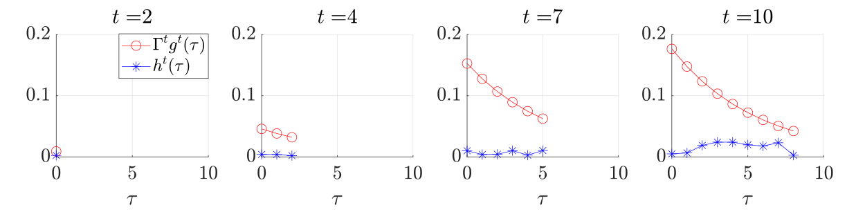
Figure 4: Verification of Assumption 3 for one face of the OV in the lane-changing example. The mean shift $h^{t}(\tau)$ in blue is upper bounded by the covariance shrinkage $\Gamma^{t}g^{t}(\tau)$ in red.

(a) Closed-loop trajectory

(b) Open-loop trajectory generated at planning steps $\tau=0,2,4,7,9$.

Figure 5: OV yield scenario in the lane-changing example. (a) The blue and magenta curves represent the closed-loop trajectories computed by the nominal and robust planners, respectively. The black polytopes are the actual positions of the OV. (b) The blue and magenta curves represent the open-loop trajectories at each planning step $\tau$ computed by the nominal and robust planners, respectively, over the planning horizon of length $T=10$. The red polytopes represent predictive samples of the OVs. During the early planning steps, the OV is predicted to exhibit two modes of behavior (i.e., yielding or accelerating). As the planning progresses and the OV’s movements are observed, these two modes converge to a single mode (i.e., yielding). Additionally, the uncertainty associated with the OV’s future states decreases over time, evidenced by the red polytopes becoming more concentrated as the planning steps advance. The nominal planner generates less conservative trajectories than the robust planner.

(a) Closed-loop trajectory

(b) Open-loop trajectory generated at planning steps $\tau=0,2,4,7,9$.

Figure 6: OV accelerate scenario in the lane-changing example. We use the same color coding as in Fig. 5.

Let the EV state be ${x}=(p_{1},p_{2},v_{1},v_{2})^{\intercal}$, where $(p_{1},p_{2})$ is the position of the centroid of the EV and $(v_{1},v_{2})$ is the velocities along the longitudinal and lateral axis of the lane boundaries, respectively. The EV is modeled as a double integrator:

$$\dot{{x}}=(\dot{p}_{1},\dot{p}_{2},\dot{v}_{1},\dot{v}_{2})^{\intercal}=(v_{1},v_{2},u_{1},u_{2})^{\intercal}.$$ (17)

Here, the input ${u}=(u_{1},u_{2})$ is the acceleration along each axis. The acceleration and velocity are bounded as $(u_{1},u_{2})\in[-10,3]\times[-5,5]$ m/s² and $(v_{1},v_{2})\in[0,22.2]\times[-5.56,5.56]$ m/s. The position $(p_{1},p_{2})$ is constrained within the boundaries of the road. To describe realistic vehicle behaviors, we impose the following coupling constraints of the acceleration and velocity:

$$\mathcal{U}\mathrel{\mathop{\mathchar 58\relax}}=\{u\in\mathbb{R}^{2}\mathrel{\mathop{\mathchar 58\relax}}|u_{1}-t_{i}|+1.3u_{2}\leq 0,\,i=1,2\},$$ (18)

$$\mathcal{X}\mathrel{\mathop{\mathchar 58\relax}}=\{x\in\mathbb{R}^{4}|\,|v_{1}-c_{i}|+2.0v_{2}\leq 0,\,i=1,2\},$$ (19)

where $t_{1}=-5.56,t_{2}=5.56,c_{1}=0$ and $c_{2}=22.2$. The initial velocity of the EV and the OV is set as 5.56 m/s. We discretize the model (17) using the zero-order hold method with sampling time $0.4$s.

At each planning step $\tau$, we minimize the cost function

$$\mathcal{J}(\textbf{x}_{\tau})=\left(x_{T_{OH},2}-x_{\text{goal}}\right)^{2}-0.1\left(x_{T_{OH},1}\right),$$ (20)

where $x_{\text{goal}}$ is the lateral center of the targeting lane. The first term encourages the lane-changing maneuver by minimizing the distance between the EV and the targeting lane. The second term motivates the forward progression of the EV by maximizing the longitudinal traveled distance. The overall planning horizon is set to be $T=10$. A shrinking-horizon planning scheme is employed, starting with $T_{OH}=10$ at the initial planning step $\tau=0$, followed by $T_{OH}=9$ at the subsequent step $\tau=1$, and so on. The risk tolerance for the chance constraint is $\epsilon=0.05$.

In this lane-changing test scene, we focus on verifying Proposition 1 and evaluating the performance of the nominal and robust planners, that is, Algorithm 1 with $\mathcal{P}$ set to (8) and (12), respectively. To validate Proposition 1, we synthesize the prediction distribution such that it satisfies Assumption 3. In particular, we let the predicted acceleration of the OV follow a multi-modal Gaussian distribution, which has two modes (yield or accelerate) at the initial planning step $\tau=0$. For the subsequent planning steps $\tau\geq 1$, the number of modes decreases to one, and we add some noise to the initial mean and multiply a decaying constant of 0.5 to the initial covariance. Fig. 4 shows the mean and covariance shifts over the planning steps $\tau$. The red curves represent the covariance shrinkage $g^{t}(\tau)$ (and multiplied by $\Gamma^{t}$) between consecutive planning steps as defined in (9), and the blue curves represent the mean shift between consecutive planning steps as defined in (10). The fact that the covariance shrinkage multiplied by $\Gamma^{t}$ is always greater than the mean shift implies that Assumption 3 is satisfied.

The simulation results are shown in Figs. 5 and 6. The predicted positions of the OV are shown in red boxes. The closed-loop trajectories generated by the nominal and robust planners are shown in blue and magenta, respectively. We conducted simulations 10 times for each scenario and then reported the average performance. The results are summarized in Table II.

Recursive feasibility: In both cases, we observed that the robust planner is recursively feasible as long as it is feasible at $\tau=0$. This confirms Proposition 1. We also observe that in the same scenarios, the nominal planner does not return Infeasible and successfully generates a closed-loop trajectory.

Optimality: We evaluate the cost function in (20) with the final state of the closed-loop trajectory, which is $\mathcal{J}(x_{T})$. The nominal planner generates a smaller cost value than the robust planner. This can also be shown in Figs. 5 and 6, where the nominal planner (the blue curves) generates less conservative trajectories, i.e., the nominal planner’s trajectory tries to cut in between the two predicted OV modes to change the lane and gain more forward progression, whereas the robust planner (the magenta curves) tries to slow down and follows behind all possible OV modes.

Computational time: We report the average worst optimization solver time across each planning step over 10 trials. Note that the two planners take a shorter computation time than the sampling time of $0.4$s, implying the real-time applicability of the proposed planners.

TABLE II: Performances in the lane-changing scenario

Method	Scene	Cost	Time (s)
Nominal ($\mathcal{P}=\eqref{problem:CLCCTPproblem}$)	OV yield	-2.56	0.15
	OV accelerate	-2.81	0.15
Robust ($\mathcal{P}=\eqref{problem:RobustMPC}$)	OV yield	0.46	0.05
	OV accelerate	-2.40	0.05

IV-B Intersection scenarios in CARLA simulator

To test the performance of our methods in real-world autonomous driving scenarios, we utilize the state-of-the-art prediction model Trajectron++ [8] and run simulations in a realistic autonomous driving CARLA simulator [27]. Also, we use ASAM OpenDRIVE that describes the road’s features, such as traffic rules in CARLA.

We consider two different scenes:

• T-intersection (T): The EV interacts with one OV at a T-intersection as shown in Fig. 7.

• Star-intersection (Star): The EV interacts with two OVs at a star-shaped intersection as shown in Fig. 8.

In the simulation, we combine shrinking-horizon planning and receding-horizon planning, as shown in Fig. 3. Before the EV enters the intersection, we neglect the OV-related chance constraints and employ receding-horizon MPC for lane keeping with an open-loop horizon $T_{s}=8$ (i.e., 4 seconds) for each MPC step. After the EV enters the intersection, we employ shrinking-horizon MPC with $T=8$, which is required to complete the turn at the intersection. We impose the chance constraints when the EV’s planned trajectories are within the intersection. We neglect the chance constraints if the OVs have already exited the intersection.

Figure 7: T-intersection scene in the CARLA simulator. The EV (red car) intends to make a left turn and reach the yellow star goal in the presence of one OV (white car).

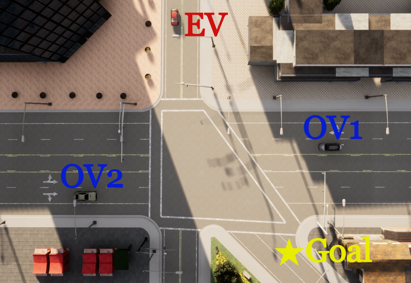
Figure 8: Star-intersection scene in the CARLA simulator. The EV (red car) intends to reach the yellow star goal. OV₁ (gray car on the right) turns to the left, and OV₂ (gray car on the left) turns to the right at the intersection.

To consider realistic vehicle motions during a turn, we use a kinematic bicycle model $\dot{x}=f(x,u)$, where

$$f(x,u)=\begin{bmatrix}v\cos(\psi+\gamma)\\ v\sin(\psi+\gamma)\\ \frac{v}{L}\cos(\gamma)\tan(u_{2})\\ u_{1}\\ \end{bmatrix}.$$ (21)

Here, $x=(p_{x},p_{y},\psi,v)$ and $u=(u_{1},u_{2})$. For the state, $(p_{x},p_{y})$ is the position in the global reference frame, $\psi$ is the angle between the vehicle’s longitudinal axis and $x$-axis of the global reference frame, and $v\in[0,15]$ m/$s$ is the velocity. For the control input, $u_{1}\in[-14,10]$ m/$s^{2}$ is the acceleration, and $u_{2}\in[-45^{\circ},45^{\circ}]$ is the steering angle. Also, $\gamma=\arctan\left(\frac{l_{r}}{L_{ov}}\tan(u_{2})\right)$ is the angle between the vehicle longitudinal axis and velocity vector, $L_{ov}=1$ m is the length of the vehicle, and $l_{r}=0.5$ m is the length between the back wheel and the vehicle center of gravity. We convert this system to a discrete-time linear time-varying (LTV) system $x_{t+1}-\bar{x}_{t+1}=A_{t}(x_{t}-\bar{x}_{t})+B_{t}(u_{t}-\bar{u}_{t})$ by linearizing (21) around a nominal trajectory $(\bar{\textbf{x}},\bar{\textbf{u}})$ [39].

(a) t = 2

(b) t = 4

(c) t = 6

(d) t = 8

(e) t = 10

(f) t = 12

Figure 9: Simulation of the nominal planner in the T-intersection scene. The EV’s trajectory (red car) is generated by the receding-horizon and shrinking-horizon implementation, and shrinking-horizon planning starts at $t=2$.

(a) t = 0

(b) t = 2

(c) t = 4

(d) t = 6

(e) t = 8

(f) t = 10

Figure 10: Simulation of the nominal planner in the star-intersection scene. Shrinking-horizon planning starts at t=0.

At each planning step $\tau$, we minimize the following quadratic cost function

$$\mathcal{J}(\textbf{u}_{\tau},\textbf{x}_{\tau})=\mathinner{\!\left\lVert{x}_{T_{OH}}-{x}_{\text{goal}}\right\rVert}_{P}^{2}+\sum^{T_{OH}-1}_{t=0}\left(\mathinner{\!\left\lVert u_{t}\right\rVert}_{R_{1}}^{2}+\mathinner{\!\left\lVert\Delta u_{t}\right\rVert}_{R_{2}}^{2}\right),$$ (22)

where $\Delta u_{t}=u_{t+1}-u_{t}$ and $P=\begin{bmatrix}300.0&0\\ 0&300.0\end{bmatrix},\;\;R_{1}=\begin{bmatrix}0.05&0.02\\ 0.02&0.10\end{bmatrix},\;\;R_{2}=\begin{bmatrix}0.05&0.01\\ 0.01&0.20\end{bmatrix}$. The first term of the objective function minimizes the terminal state distance to the goal state. To promote smooth and stable driving behavior, the second term minimizes both the magnitude of acceleration and steering interventions and the differences in control inputs across consecutive time steps.

The prediction model Trajectron++ [8] generates $N_{s}$ samples of OV trajectory predictions. Each sample has an associated discrete latent variable, which encodes an associated GMM mode. We determine the number of modes based on the discrete latent variables’ values that exceed a certain threshold; for example, $K=2$ at the beginning of shrinking-horizon planning in the T-intersection scene, and $K_{1}=3,K_{2}=3$ at the beginning of shrinking-horizon planning in the star-intersection scene. Then, we cluster the samples according to their latent variable’s value, obtaining $N_{k}$ samples for each mode $k$ and estimating the GMM moments from the $N_{k}$ samples. The risk tolerance for the chance constraint (6) is $\epsilon=0.05$.

Under the predictions from Trajectron++, Assumption 3 does not always hold. The predictions corresponding to OV-turning exhibit substantial mean shifts for consecutive time steps, making the fulfillment of Assumption 3 impractical. Also, the covariance of predictions occasionally exhibits irregular increases or decreases in magnitude. These violations make it difficult to validate Proposition 1 with the prediction model. Improving the predictions’ quality can help alleviate these violations, which could be considered as future work.

We implement the nominal, robust, and contingency MPC planners, that is, Algorithm 1 with $\mathcal{P}$ set to (8), (12), and (16), respectively. For contingency planning, we use a coinciding horizon $T_{c}=1$ and plan $L$ trajectories. Each plan accounts for different combinations of chance constraints. For instance, when OV₁ has three modes and OV₂ has two modes, we plan $L=3$ trajectories where $\textbf{u}^{(1)}$ handles the chance constraints of the first modes of OV₁ and OV₂, $\textbf{u}^{(2)}$ the second modes of OV₁ and OV₂, and $\textbf{u}^{(3)}$ the third mode of OV₁.

We conducted 100 trials of simulations for each scenario; in each trial, shrinking-horizon planning is initially feasible. In each trial, the OVs start from the same initial states, yet their accelerations, steering inputs, and intentions (e.g., going straight or turning right at the T-intersection) vary in different trials. One exemplary trial of the nominal planner for the T-intersection scene is shown in Fig. 9 and for the star-intersection scene in Fig. 10. We compare the performance of the three planners introduced in Section III with several criteria, and the results are summarized in Table III.

Open-loop & closed-loop planning: We first evaluate the improvement brought by employing our MPC framework in comparison to open-loop planning. In particular, the open-loop planner tries to generate a trajectory by solving the trajectory planning problem just once at the very initial planning step, i.e., solving either nominal planning (8) or contingency planning (16) with $\tau=0$ and $T_{OH}=T$ that is the required planning horizon length to reach the goal. The open-loop planning scheme cannot find a feasible solution in all scenes due to the highly uncertain OV prediction over a long planning horizon (as shown in the last row of Table III). On the other hand, the MPC framework overcomes this infeasibility by gaining new observations of the OVs’ motion and correspondingly updating the OV predictions and EV trajectories at each planning step.

Feasibility: As for the feasibility criteria, we count the number of trials where each planner returns Infeasible before the EV reaches the goal. For example, if the feasibility is 83% (nominal planner in the T-intersection scene), it indicates that the nominal planner generates a closed-loop trajectory in 83 trials out of the total 100 trials.

We observe that both the nominal and contingency planners have a high feasibility rate in the two scenes, while the robust planner has a lower feasibility rate. As we noted earlier in this section, the robust planner does not have a recursive feasibility guarantee because the predictions from Trajectron++ do not satisfy Assumption 3. At the star intersection, the nominal planner has a higher feasibility rate than the contingency planner. The reason is that the contingency planner tends to make aggressive maneuvers in the early steps of MPC and may fail to find a feasible trajectory in the subsequent steps. The robust planner cannot find a feasible closed-loop solution in the star-intersection scene due to the high interaction and highly uncertain predictions of the OVs.

Optimality: As for the optimality criteria, we evaluate the average cost and the traveled time. The cost value of each feasible trial is calculated based on (22) over the planning horizon until the EV reaches the goal. In the column of “Cost” of Table III, we report the average cost values over feasible trials. The travel time refers to the average time taken for the EV to reach the goal from its initial state. We summarize the average travel time among the feasible trials in the column of “Travel time” of Table III. Our objective is to minimize the cost, and typically, a lower cost results in fewer planning steps needed to reach the goal.

In both scenes, the contingency planner has the best performance in terms of minimizing the cost, followed by the nominal planner. The robust planner generates trajectories with much higher cost and travel time. For example, at the T-intersection, the EV driven by the robust planner fully stops to wait for the OVs to exit the intersection, thereby taking a long time to reach the goal, whereas the EV only slows down with the nominal and contingency planners.

TABLE III: Performances in the intersection scenarios

Method	Scene	Feasibility	Travel time	Cost	Comp. time
Nominal ($\mathcal{P}=\eqref{problem:CLCCTPproblem}$)	T	83%	6.82s	6526	3.43s
	Star	92%	5.29s	5382	3.27s
Robust ($\mathcal{P}=\eqref{problem:RobustMPC}$)	T	70%	8.53s	21000	2.72s
	Star	0%	-	-	-
Contingency ($\mathcal{P}=\eqref{problem:contingencyMPC}$)	T	93 %	6.51s	4156	14.1s
	Star	85%	5.06s	3760	10.1s
Open-loop	All scenes	0%	-	-	-

Computational time: To evaluate how close our methods are to real-time applicability, we measure the worst optimization solver time taken to solve $\mathcal{P}$ of Algorithm 1 in each trial. We report the average worst time over 100 trials in the column of “Comp. time” in Table III. The contingency planner has the longest computational time as it plans $L$ trajectories simultaneously.

Given that we solve the trajectory planning problem at a frequency of every 0.5 s, the computational time of our planners cannot satisfy the real-time applicability. In comparison with the previous chance-constrained MPC framework under GMM uncertainty in [21], which offers real-time applicability, a key difference is that in [21], the lane-keeping behavior is tackled by planning a trajectory that closely aligns with a reference trajectory that is computed offline. In contrast, our approaches incorporate lane-keeping as a constraint, where we force the state to stay within (curved) lane boundaries described by the union of convex sets. We believe that the computation time can be further reduced by reformulating the lane-keeping constraints and optimizing the codes, which remains as a future work.

In summary, the realistic simulations indicate that our proposed methods can ensure safety while conservativeness and/or computation time can be a tradeoff. In particular, the robust planner offers a provable recursive feasibility guarantee but tends to generate conservative trajectories. The less conservative planning of the contingency planner comes at the price of increased computation time. The nominal planner appears to offer both recursive feasibility and safety throughout our simulation trials.

V Conclusion

We presented a chance-constrained MPC framework that considers GMM uncertainty. With assumptions on the propagation of the uncertainty’s GMM prediction, we ensured that a robust MPC planner is recursively feasible and safe with respect to the chance constraint throughout the entire planning horizon. A less conservative chance-constrained MPC planner was designed based on a contingency planning method, which reduces the conservativeness under GMM uncertainty by planning multiple trajectories simultaneously. Through a case study using a cutting-edge autonomous driving simulator, we observed that the MPC framework removes the conservatism of open-loop controllers in finite-horizon trajectory planning problems. While the contingency planning approach enhanced the trajectory’s optimality, it came at the expense of extended computational time. Our planning framework requires further improvement in terms of computation time to support real-time applications. Moreover, enhancing the prediction quality of other vehicles can reduce the conservativeness of risk-constrained problems.

References

- [1] A. Majumdar and M. Pavone, “How Should a Robot Assess Risk? Towards an Axiomatic Theory of Risk in Robotics,” 2017.
- [2] A. Hakobyan, G. C. Kim, and I. Yang, “Risk-Aware Motion Planning and Control Using CVaR-Constrained Optimization,” IEEE Robotics and Automation Letters, vol. 4, no. 4, pp. 3924–3931, 2019.
- [3] F. S. Barbosa, B. Lacerda, P. Duckworth, J. Tumova, and N. Hawes, “Risk-Aware Motion Planning in Partially Known Environments,” in 60th IEEE Conference on Decision and Control, 2021, pp. 5220–5226.
- [4] G. C. Calafiore and L. El Ghaoui, “On Distributionally Robust Chance-Constrained Linear Programs,” Jour. of Optimization Theory and Applications, vol. 130, no. 1, Dec. 2006.
- [5] L. Blackmore, M. Ono, and B. C. Williams, “Chance-Constrained Optimal Path Planning With Obstacles,” IEEE Transactions on Robotics, vol. 27, no. 6, pp. 1080–1094, 2011.
- [6] S. Jha, V. Raman, D. Sadigh, and S. A. Seshia, “Safe Autonomy Under Perception Uncertainty Using Chance-Constrained Temporal Logic,” Journal of Automated Reasoning, vol. 60, no. 1, pp. 43–62, 2018.
- [7] A. Ahmadi-Javid, “Entropic Value-at-risk: A New Coherent Risk Measure,” Journal of Optimization Theory and Applications, vol. 155, no. 3, p. 1105–1123, 2011.
- [8] T. Salzmann, B. Ivanovic, P. Chakravarty, and M. Pavone, “Trajectron++: Dynamically-feasible Trajectory Forecasting with Heterogeneous Data,” Computer Vision – ECCV 2020, p. 683–700, 2020.
- [9] N. Rhinehart, R. Mcallister, K. Kitani, and S. Levine, “PRECOG: PREdiction Conditioned on Goals in Visual Multi-Agent Settings,” in 2019 IEEE/CVF International Conference on Computer Vision (ICCV). IEEE Computer Society, 2019, pp. 2821–2830.
- [10] Z. Hu, W. Sun, and S. Zhu, “Chance Constrained Programs with Gaussian Mixture Models,” IISE Transactions, pp. 1–14, 2022.
- [11] L. You, H. Ma, T. K. Saha, and G. Liu, “Gaussian Mixture Model Based Distributionally Robust Optimal Power Flow With CVaR Constraints,” 2021.
- [12] P. Mohajerin Esfahani and D. Kuhn, “Data-driven Distributionally Robust Optimization Using the Wasserstein Metric: Performance Guarantees and Tractable Reformulations,” Mathematical Programming, vol. 171, no. 1–2, p. 115–166, 2017.
- [13] A. Hakobyan and I. Yang, “Wasserstein Distributionally Robust Motion Control for Collision Avoidance Using Conditional Value-at-Risk,” IEEE Transactions on Robotics, vol. 38, no. 2, pp. 939–957, 2022.
- [14] H. Ahn, C. Chen, I. M. Mitchell, and M. Kamgarpour, “Safe Motion Planning Against Multimodal Distributions Based on a Scenario Approach,” IEEE Control Systems Letters, vol. 6, p. 1142–1147, 2022.
- [15] G. Calafiore and M. Campi, “The Scenario Approach to Robust Control Design,” IEEE Transactions on Automatic Control, vol. 51, no. 5, pp. 742–753, 2006.
- [16] M. C. Campi, S. Garatti, and M. Prandini, “The Scenario Approach For Systems and Control Design,” Annual Reviews in Control, vol. 33, no. 2, p. 149–157, 2009.
- [17] K. Ren, H. Ahn, and M. Kamgarpour, “Chance-Constrained Trajectory Planning With Multimodal Environmental Uncertainty,” IEEE Control Systems Letters, vol. 7, pp. 13–18, 2023.
- [18] C. E. Garcia, D. M. Prett, and M. Morari, “Model Predictive Control: Theory and Practice.” Autom., vol. 25, no. 3, pp. 335–348, 1989.
- [19] A. T. Schwarm and M. Nikolaou, “Chance-constrained Model Predictive Control,” AIChE Journal, vol. 45, no. 8, p. 1743–1752, 1999.
- [20] A. Mesbah, “Stochastic Model Predictive Control: An Overview and Perspectives for Future Research,” IEEE Control Systems Magazine, vol. 36, no. 6, pp. 30–44, 2016.
- [21] S. H. Nair, V. Govindarajan, T. Lin, C. Meissen, H. E. Tseng, and F. Borrelli, “Stochastic MPC with Multi-modal Predictions for Traffic Intersections,” in 2022 IEEE 25th International Conference on Intelligent Transportation Systems (ITSC), 2022, pp. 635–640.
- [22] E. Kerrigan and J. Maciejowski, “Invariant Sets for Constrained Nonlinear Discrete-time Systems with Application to Feasibility in Model Predictive Control,” Proceedings of the 39th IEEE Conference on Decision and Control, 2000.
- [23] G. Schildbach, L. Fagiano, C. Frei, and M. Morari, “The Scenario Approach for Stochastic Model Predictive Control with Bounds on Closed-loop Constraint Violations,” Automatica, vol. 50, no. 12, p. 3009–3018, 2014.
- [24] B. Kouvaritakis and M. Cannon, “Stochastic Model Predictive Control,” Encyclopedia of Systems and Control, p. 2190–2196, 2021.
- [25] Y. Kuwata, J. Teo, G. Fiore, S. Karaman, E. Frazzoli, and J. P. How, “Real-Time Motion Planning With Applications to Autonomous Urban Driving,” IEEE Transactions on Control Systems Technology, vol. 17, no. 5, pp. 1105–1118, 2009.
- [26] J. Hardy and M. Campbell, “Contingency Planning Over Probabilistic Obstacle Predictions for Autonomous Road Vehicles,” IEEE Transactions on Robotics, vol. 29, no. 4, pp. 913–929, Aug. 2013.
- [27] A. Dosovitskiy, G. Ros, F. Codevilla, A. Lopez, and V. Koltun, “CARLA: An Open Urban Driving Simulator,” in Proceedings of the 1st Annual Conference on Robot Learning, 2017, pp. 1–16.
- [28] T. R. Rockafellar and S. P. Uryasev, “Conditional Value-at-Risk for General Loss Distributions,” SSRN Electronic Journal, 2001.
- [29] C. Bishop, Pattern Recognition and Machine Learning. Springer, 2006.
- [30] V. Lefkopoulos and M. Kamgarpour, “Trajectory Planning Under Environmental Uncertainty With Finite-sample Safety Guarantees,” Automatica, vol. 131, p. 109754, Sep 2021.
- [31] A. Dixit, M. Ahmadi, and J. W. Burdick, “Risk-Sensitive Motion Planning using Entropic Value-at-Risk,” in 2021 European Control Conference (ECC), 2021, pp. 1726–1732.
- [32] T. Schouwenaars, B. De Moor, E. Feron, and J. How, “Mixed Integer Programming for Multi-vehicle Path Planning,” in 2001 European Control Conference (ECC), 2001, pp. 2603–2608.
- [33] G. Casella and R. Berger, Statistical Inference. Duxbury Resource Center, June 2001.
- [34] F. Borrelli, A. Bemporad, and M. Morari, Predictive Control for Linear and Hybrid Systems, 1st ed. USA: Cambridge University Press, 2017.
- [35] M. Lorenzen, F. Dabbene, R. Tempo, and F. Allgöwer, “Constraint-Tightening and Stability in Stochastic Model Predictive Control,” IEEE Transactions on Automatic Control, vol. 62, no. 7, pp. 3165–3177, 2017.
- [36] Y. Yoon, T. Kim, H. Lee, and J. Park, “Road-Aware Trajectory Prediction for Autonomous Driving on Highways,” Sensors, vol. 20, no. 17, 2020.
- [37] Gurobi Optimization, LLC, “Gurobi Optimizer Reference Manual,” 2023. [Online]. Available: https://www.gurobi.com
- [38] I. I. Cplex, “V12. 1: User’s Manual for CPLEX,” International Business Machines Corporation, vol. 46, no. 53, p. 157, 2009.
- [39] P. Falcone, M. Tufo, F. Borrelli, J. Asgari, and H. E. Tseng, “A Linear Time-Varying Model Predictive Control Approach to the Integrated Vehicle Dynamics Control Problem in Autonomous Systems,” in 2007 46th IEEE Conference on Decision and Control, 2007, pp. 2980–2985.