Anomalous diffusion of the heavy quarks through the fractional Langevin equation

Abstract

The dynamics of heavy quarks within the hot QCD medium have been revisited, considering the influence of anomalous diffusion. This study has been conducted using the framework of the fractional Langevin equation involving the Caputo fractional derivative. We introduce a numerical scheme for the fractional Langevin equation and demonstrate that the mean square displacement of the particle exhibits anomalous diffusion, deviating from a linear relationship with time. Our analysis calculates various entities, such as mean squared momentum, momentum spread, and the nuclear suppression factor, $R_{AA}$. Notably, our findings indicate that superdiffusion strongly suppresses the $R_{AA}$ compared to normal diffusion in the hot QCD medium. The possible impacts on other parameters are also discussed.

I Introduction

The ultra-relativistic heavy-ion collisions (HICs) at the Relativistic Heavy-Ion Collider (RHIC) and the Large Hadron Collider (LHC) have predicted the existence of Quark-Gluon Plasma (QGP); a state of matter where quarks and gluons are free to move beyond the nucleonic volume Adams et al. (2006, 2005); Adcox et al. (2005); Aamodt et al. (2010); Arsene et al. (2005). The QGP is short-lived, with an expected lifespan of a few fm/c (approximately 4-5 fm/c at RHIC and 10-12 fm/c at LHC  van Hees and Rapp (2005); Rapp and van Hees (2010)). Conversely, investigating the characteristics of the QGP by studying the dynamics of heavy quarks (charm and beauty) is a subject of significant interest. In this context, The heavy quarks (HQs) serve as prominent probes of QGP Song et al. (2015); Andronic et al. (2016); Dong and Greco (2019); Cao et al. (2019); Beraudo et al. (2018); Prino and Rapp (2016); Aarts et al. (2017); Uphoff et al. (2011); Golam Mustafa et al. (1998); Plumari et al. (2018); Gossiaux and Aichelin (2008); Prakash et al. (2021, 2023); Prakash and Jamal (2023a); Jamal et al. (2023); Singh et al. (2023); Kurian et al. (2020); Cao et al. (2016); Mazumder et al. (2011); Zhang et al. (2023); Jamal et al. (2021); Jamal and Mohanty (2021a, b); Sun et al. (2023); Plumari et al. (2020); Prakash and Jamal (2023b); Debnath et al. (2023); Du and Qian (2023); Shaikh et al. (2021); Kumar et al. (2022); Das et al. (2022). Due to their large masses ($M_{c}/M_{b}$ $\sim$ 1.3/4.5 GeV), HQs are generated at the early stages of HICs. Moreover, the thermalization of the HQs is delayed compared to the light partons of the bulk medium by a factor on the order of $\sim$ $M/T$. This delay renders the thermalization time of the HQs comparable to the lifetime of the QGP fireball. Since the HQs are not expected to achieve complete thermalization, they retain the memory of their interaction history. Hence, they serve as a novel probe for observing the complete evolution of the QGP medium and act as non-equilibrium entities within the equilibrated QGP. The standard Langevin equation (LE) is used to study Brownian motion under the assumption of normal diffusion, which means a linear increase in the mean-square displacement of the particle with time for a sufficiently large time Kubo et al. (2012). By using the Langevin equation Young et al. (2012); Lang et al. (2016); Cao and Bass (2011); van Hees et al. (2008); Das et al. (2014) in the context of the HQs momentum and position evolution in the hot QCD medium and numerous studies available for the experimental observables related to the HQs, such as the nuclear suppression factor, $R_{AA}$ and elliptic flow, $v_{2}$ He et al. (2023, 2012); Das et al. (2015); Zhang et al. (2023). Several processes exhibit anomalous diffusion, a phenomenon where the mean squared displacement of the particle does not vary linearly with time as predicted by Einstein’s law. Specifically, anomalous diffusion is characterized by a non-standard time dependence of the mean squared displacement ($\langle x(t)^{2}\rangle$) written as follows Balescu (1995); Bouchaud and Georges (1990); Metzler and Klafter (2000); Caspi et al. (2000); Weber et al. (2010); Vitali et al. (2018); Oliveira et al. (2019); Sokolov and Klafter (2005); Lutz (2001); Lim and Teo (2009); Wang and Chen (2023),

$$\langle x(t)^{2}\rangle\propto t^{\mu},\ {\mu}\neq 1,$$ (1)

where $t$ is the evolution time of the particle. The process describes normal diffusion, corresponding to the case where ${\mu}=1$. Subdiffusion occurs when ${\mu}<1$, whereas superdiffusion occurs when ${\mu}>1$ Metzler and Klafter (2000). Despite the crucial role played by the LE across several fields, it fails to accurately describe certain behaviours, such as anomalous diffusion (i.e., superdiffusion and subdiffusion). Therefore, fractional Langevin equations (FLE) have been proposed to study anomalous diffusion Li et al. (2012); Kobelev and Romanov (2000); Coffey et al. (2004). Mainardi et al., Gorenflo and Mainardi (1997); Mainardi and Pironi (1996); Mainardi (1997) introduced an FLE in their groundbreaking research. The Langevin method has primarily been applied to study anomalous diffusion using Caputo fractional derivative Guo et al. (2013); Li and Zeng (2013); Miller and Ross (1993). On the other hand, there are several distinct formulations for fractional derivatives, such as Riemann-Liouville derivative Carpinteri and Mainardi (2014), Riesz derivative Agrawal (2007), Feller derivative Feller (1971), and others. In the subsequent, we will only use the Caputo fractional derivative in our analysis to study the anomalous diffusion of the particle in the medium.

Another valuable approach to studying anomalous diffusion involves the investigation of the fractional diffusion equation, fractional Fokker-Planck equation Metzler et al. (1999), and generalized Chapman-Kolmogorov equation Metzler (2000). Anomalous diffusion has been used in many fields, including molecular chemistry Zumofen and Klafter (1994), biology Lomholt et al. (2005), and anomalous diffusion, polymer transport theory Shlesinger et al. (1993). Also, when accounting for interactions between the Brownian particle and the constituent particles of the medium, the fluctuations are influenced by their prior states, a phenomenon termed as memory. The current movement is affected by previous movements via a memory kernel in the generalized Langevin equation. Such memory effects can result in anomalous diffusion for a particular memory time Wang and Tokuyama (1999); Wang (1992a); Porrà et al. (1996); Wang (1992b); Fa (2006); Siegle et al. (2010); Chen et al. (2023, 2023) and also plays a role in the QGP Hammelmann et al. (2019); Kapusta et al. (2012); Ruggieri et al. (2022); Pooja et al. (2023).

Recently, the transverse momentum broadening of a fast parton via superdiffusion in the QCD matter has been studied in Ref. Caucal and Mehtar-Tani (2022). With this motivation for the applications of superdiffusion on the HQs dynamics in hot QCD matter, we use FLE, a generalized form of the LE. Unlike the LE, the FLE replaces integer-order derivatives with fractional-order derivatives, specifically of Caputo type Caputo (1967). This may be the first attempt where we present an anomalous diffusion for the HQ dynamics in the QGP medium. In this article, we specifically study the effect of superdiffusion on the HQ dynamics in the QGP medium. The subdiffusion is not considered within the scope of the current analysis.

We anticipate a key outcome in our study, specifically that in the presence of superdiffusion, there will be an increase in the energy loss experienced by the HQs within the QGP medium. This conclusion is confirmed by studying various key parameters, including the mean squared displacement, mean squared momentum, momentum spread, $dN/dp_{T}$, and the $R_{AA}$ of the HQs. Notably, the latter holds particular significance in the phenomenology of the HQs within the QGP. The strong suppression observed in $R_{AA}$ is anticipated to contribute significantly to developing a substantial elliptic flow ($v_{2}$) for the HQs.

The article is structured as follows: Section II introduces the formalism; we analytically solve the FLE of non-relativistic heavy particles using the Laplace technique, along with presenting a numerical scheme for solving the relativistic FLE. Section III is dedicated to the presentation of our results. Lastly, Section IV provides a comprehensive summary of our conclusions.

II The fraction Langevin equation for Brownian particles

For illustrative purposes, we discuss the scenario of a heavy particle with mass $M$ undergoing one-dimensional (1-D) motion within the nonrelativistic limit. We use the FLE to describe the dynamics of this particle. In this framework, the evolution of the particle’s position and momentum is characterized by fractional derivatives of orders $\beta$ and $\alpha$ Kobelev and Romanov (2000); Li et al. (2012),

$${}^{C}D^{\beta}_{0+}x(t)=\frac{p(t)}{M},$$ (2)

$${}^{C}D^{\alpha}_{0+}p(t)=-\gamma p(t)+\xi(t),$$ (3)

where the momentum of a particle at time $t$ is denoted as $p(t)$, its position as $x(t)$. ${}^{C}D_{0+}^{\alpha}$ denotes Caputo fractional derivative, $\alpha$ and $\beta$ are the fractional parameter, with $n-1<\alpha\leq n$, and ${}^{C}D_{0+}^{\beta}$ with $n-1<\beta\leq n$, $n\in\mathbb{N}$ ($n$ is a natural number). Brownian particle encounters two distinct forces: the dissipative force, characterized by the drag coefficient, denoted by $\gamma$, and the stochastic force, denoted as $\xi(t)$. The latter governs the random noise, commonly referred to as white Gaussian noise. White noise gives rise to a fluctuating field without memory, characterized by instantaneous decay in correlations of the white noise, often referred to as a $\delta$ correlation. The random force satisfies certain properties, such as:

$$\langle\xi(t)\xi(t^{\prime})\rangle=2\mathcal{D}\delta(t-t^{\prime}),$$ (4)

$$\langle\xi(t)\rangle=0,$$ (5)

$\mathcal{D}$ is the diffusion coefficient of the heavy particle in a medium of temperature, $T$. The drag coefficient ($\gamma$) is related to the diffusion coefficient through the Fluctuation-Dissipation Theorem (FDT) as follows:

$$\gamma=\frac{\mathcal{D}}{MT}.$$ (6)

The Caputo fractional derivative Caputo (1967) is defined as,

$$^{C}D^{\nu}_{0+}u(t)=\frac{1}{\Gamma({n-\nu})}\int_{0}^{t}\frac{u^{(n)}(s)}{(t-s)^{1+\nu-n}}ds,$$ (7)

where $u^{(n)}$ denotes the $n^{th}$ derivative of $u$. The fractional derivative which corresponds to the superdiffusion, i.e., when $1<\nu\leq 2$, is given by

$$^{C}D^{\nu}_{0+}u(t)=\frac{1}{\Gamma({2-\nu})}\int_{0}^{t}\frac{u^{(2)}(s)}{(t-s)^{\nu-1}}ds,$$ (8)

where $\Gamma(\cdot)$ denotes the gamma function. In the following subsection, we solve analytically the FLE of non-relativistic Brownian particles.

II.1 Analytical solutions

Analytically, we solve the FLE governing the motion of non-relativistic Brownian particles. To achieve this, we use the Laplace technique, providing analytical expressions for $\langle p^{2}(t)\rangle$ and $\langle x^{2}(t)\rangle$. Performing the Laplace transformation of Caputo derivative for $n-1<\alpha\leq n$ and $n-1<\beta\leq n$ Podlubny ,

$$\mathcal{L}\left[{}^{C}D^{\alpha}_{0+}p(t)\right](z)=z^{\alpha}\widehat{p}(z)-\sum_{k=0}^{n-1}z^{\alpha-k-1}\left[p^{k}(0)\right].$$ (9)

In order to calculate the solution of $p(t)$ and $x(t)$ of the heavy particle for a super-diffusive process, i.e., when $1<\alpha\leq 2$ and $1<\beta\leq 2$, one can take the Laplace transform Eqs. (2), (3) and using Eq. (9), it can be obtained easily as

$$z^{\beta}\widehat{x}(z)-z^{\beta-1}x(t_{0})-z^{\beta-2}x^{\prime}(t_{0})=\frac{\widehat{p}(z)}{M},$$ (10)

$$\widehat{p}(z)=\frac{z^{\alpha-1}}{z^{\alpha}+\gamma}p(t_{0})+\frac{z^{\alpha-2}}{z^{\alpha}+\gamma}p^{\prime}(t_{0})+\frac{\widehat{\xi}(z)}{z^{\alpha}+\gamma}.$$ (11)

Now, substituting Eq. (11) into Eq. (10), for simplicity, we take $M=1$ Sandev et al. (2012), we obtain

$$\widehat{x}(z)= \;\frac{x(t_{0})}{z}+\frac{x^{\prime}(t_{0})}{z^{2}}+\frac{z^{\alpha-\beta-1}}{z^{\alpha}+\gamma}p(t_{0})+\frac{z^{\alpha-\beta-2}}{z^{\alpha}+\gamma}p^{\prime}(t_{0})$$

$$+\frac{z^{-\beta}}{z^{\alpha}+\gamma}\widehat{\xi}(z).$$ (12)

Taking the inverse Laplace transform of Eqs. (11) and (II.1), we obtain

$$p(t)= \;E_{\alpha,1}(-\gamma t^{\alpha})p(t_{0})+tE_{\alpha,2}(-\gamma t^{\alpha})p^{\prime}({t_{0}})$$

$$+\int_{0}^{t}(t-s)^{\alpha-1}E_{\alpha,\alpha}(-\gamma(t-s)^{\alpha})\xi(s)ds,$$ (13)

and

$$x(t)= \;x_{0}+tx^{\prime}_{0}+t^{\beta}E_{\alpha,\beta+1}(-\gamma t^{\alpha})p(t_{0})$$

$$+t^{\beta+1}E_{\alpha,\beta+2}(-\gamma t^{\alpha})p^{\prime}({t_{0}})$$

$$+\int_{0}^{t}(t-s)^{\beta+\alpha-1}E_{\alpha,\beta+\alpha}(-\gamma(t-s)^{\alpha})\xi(s)ds,$$ (14)

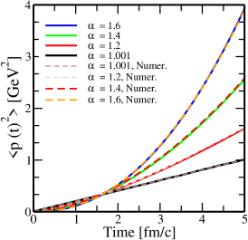
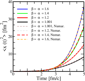
Figure 1: $\langle p^{2}(t)\rangle$ versus time (left panel) and $\langle x^{2}(t)\rangle$ versus time (right panel) for a 1-D, purely diffusive motion for different values of $\alpha$ and $\beta$. Analytic solutions are represented by solid lines, and numerical (Numer.) solutions are represented by dashed lines.

where

$$E_{\alpha,\beta}(z)=\sum^{\infty}_{j=0}\frac{z^{j}}{\Gamma(j\alpha+\beta)}$$

is the two-parameter Mittag-Leffler function for $\alpha>0$, $\beta>0$, and $z$ is a complex number Erdélyi et al. (1953) and the Laplace transform of the two-parameter Mittag-Leffler function is Hilfer (2000),

$$\mathcal{L}\left[x^{\beta-1}E_{\alpha,\beta}(-\lambda x^{\alpha})\right](z)=\frac{z^{\alpha-\beta}}{z^{\alpha}+\lambda}.$$ (15)

Next we calculate $\langle p^{2}(t)\rangle$, and $\langle x^{2}(t)\rangle$ analytically for the Brownian particle.

II.1.1 Purely diffusive motion

We are calculating the $\langle p^{2}(t)\rangle$, and $\langle x^{2}(t)\rangle$ for a purely diffusive (when $\gamma=0$ in the FLE), 1-D motion. Then Eq. (3) simplified to

$${}^{C}D^{\alpha}_{0+}p(t)=\xi(t),$$ (16)

with initial momentum, $p(t_{0})=0$. Then to calculate $\langle p^{2}(t)\rangle$ we follows Eq. (13) and Eq. (16), then we get

$$\langle p^{2}(t)\rangle=\frac{1}{\Gamma(\alpha)^{2}}\int_{0}^{t}\int_{0}^{t}(t-s_{1})^{\alpha-1}(t-s_{2})^{\alpha-1} \langle\xi(s_{1})\xi(s_{2})\rangle$$

$$ds_{1}ds_{2}.$$ (17)

Solving further Eq. (II.1.1), using the correlation properties defined in Eq. (4), we have,

$$\langle p^{2}(t)\rangle =\frac{2\mathcal{D}}{\Gamma(\alpha)^{2}}\int_{0}^{t}(t-s)^{2\alpha-2}ds,$$ (18)

$$\langle p^{2}(t)\rangle =\frac{2\mathcal{D}}{\Gamma(\alpha)^{2}}\frac{t^{2\alpha-1}}{2\alpha-1}.$$ (19)

Similarly, one can calculate analytical solutions of $\langle x^{2}(t)\rangle$ for $\gamma=0$, and with initial conditions, $x(t_{0})=0$, using Eqs. (II.1),  (16) as

$$\langle x^{2}(t)\rangle\approx \;\frac{2\mathcal{D}}{\Gamma(\alpha+\beta)^{2}}\int_{0}^{t}(t-s)^{2\alpha+2\beta-2}ds$$

$$=\frac{2\mathcal{D}}{\Gamma(\alpha+\beta)^{2}}\frac{t^{2\alpha+2\beta-1}}{2\alpha+2\beta-1}.$$ (20)

We have plotted Fig. 1 for the case of purely diffusive motion, we depict the variation of $\langle p^{2}(t)\rangle$ over time (left panel) and $\langle x^{2}(t)\rangle$ (right panel), each for different values of $\alpha$ and $\beta$, while keeping $\mathcal{D}$ constant at $0.1$ GeV²/fm. For simplicity, a non-relativistic case has been considered with $M=1$ GeV. In Fig. 1 (left panel), results obtained from Eq. (19) show that $\langle p^{2}(t)\rangle$ exhibits nearly linear evolution with time when $\alpha\rightarrow 1$ (as shown by black solid lines), which is giving $\langle p^{2}(t)\rangle=2\mathcal{D}t$. In this scenario, the Caputo fractional derivative reduces to an ordinary first-order derivative; in this limit of $\alpha$, the FLE is reduced back to the LE. On the other hand, when the value of $\alpha>1$, the linear increase in $\langle p^{2}(t)\rangle$ with time converts into nonlinear growth over time. It becomes evident that the diffusion process evolves more gradually during the initial time, particularly up to $1.5$ fm/c. In contrast, around $2$ fm/c, the pattern is reversed, now a higher value of $\alpha$, giving a faster diffusion. Similarly, with the same input parameter, Fig. 1 (right panel) results obtained from Eq. (20) depicts the mean square displacement, $\langle x^{2}(t)\rangle$ varies with time. In the limit, $\alpha,\beta\rightarrow 1$(as shown by black solid lines), $\langle x^{2}(t)\rangle$ varies with $t^{3}$ (as shown by black solid lines), showing the normal diffusion. However, with value higher values of $\alpha$ and $\beta$, $\langle x^{2}(t)\rangle$ varies with the power of time greater than cubic power.

II.2 A numerical scheme for the fractional Langevin equation

In classical stochastic differential equations driven by Brownian motion, the Itô or Stratonovich stochastic calculus is typically employed for solutions. However, these methods are not applicable to the FLE driven by fractional Brownian motion, as it is not a semimartingale (see Ref. Rogers (1997) for detailed proof). Although the Monte Carlo method is a reliable solution for stochastic differential equations, it is not appropriate in this case because it relies on independent sequences. Still, the sequences in fractional noise are dependent. Therefore, we have employed L2 numerical schemes, as detailed in Oldham and Spanier (1974). These schemes are among the most effective for discretizing the Caputo fractional derivative and provide a key contribution to this article. We numerically solve the FLE in Eqs. (2), (3). To validate our numerical computations, we compared the numerical results with the analytical ones for the 1-D FLE, considering $\gamma$ = 0. This step is crucial to ensure the accuracy of our numerical method, which will be employed in solving the relativistic Langevin equation that will be discussed in the following subsection. To solve the FLE, numerical methods are commonly categorized as indirect or direct. Since time-fractional differential equations can generally be reformulated into integro-differential equations, solving such equations corresponds to indirect methods. On the other hand, direct methods focus on approximating the time-fractional derivative itself. This aspect constitutes the core of our work, where our goal is to discretize the fractional derivative directly without transforming the associated differential equation into its integral form. Our numerical algorithm for solving the FLE is based on the three-step scheme using the central difference method shown in Appendix VI.

II.2.1 The fractional Langevin equation of relativistic Brownian particles: QGP

We extended the solution of FLE defined in Eqs. (2),(3), to describe the HQs dynamics in the QGP medium in the relativistic limit as follows,

$${}^{C}D^{\beta}_{0+}x(t)=\frac{p(t)}{E(t)},$$ (21)

$${}^{C}D^{\alpha}_{0+}p(t)=-\gamma p(t)+\xi(t),$$ (22)

where, $E=\sqrt{p^{2}+M^{2}}$ represents the energy, and $p$ denotes the momentum of the HQs. The $\gamma$ can be related to the diffusion coefficient through an FDT as Walton and Rafelski (2000); Moore and Teaney (2005); Mazumder et al. (2014),

$$\gamma=\frac{\mathcal{D}}{ET}.$$ (23)

Since both Eq. (21) and Eq. (22) are non-linear differential integral equations, preventing analytical solutions through methods such as Laplace transformations, as done for the non-relativistic case for Eqs. (2),(3). The solution of relativistic FLE defined in Eq. (22) and Eq. (21) is possible solely through numerical methods. We utilize the numerical approach to compute $\langle x^{2}(t)\rangle$, $\langle p^{2}(t)\rangle$, the momentum distribution, and $R_{AA}$ of the HQs. For superdiffusion, the relativistic FLE can be written in the discrete form using Eq. (30) ( given in appendix VI) as follows,

$$\begin{cases}x(t_{1})=x(t_{0})+\left[\displaystyle\frac{p(t_{0})}{E(t_{0})}\right]k\;&:\;n=1,\\ x(t_{2})=2x(t_{1})-x(t_{0})+\left[\displaystyle\frac{p(t_{1})}{E(t_{1})}\right]k\;&:\;n=2,\\ x(t_{n})=2x(t_{n-1})-x(t_{n-2})+\Bigg{[}\displaystyle\frac{p(t_{n-1})}{E(t_{n-1})}&\\ -\displaystyle\sum_{j=1}^{n-2}b_{j}\left(x(t_{n-j})-2x(t_{n-j-1})+x(t_{n-j-2})\right)+\displaystyle\frac{n^{2-\alpha}-(n-1)^{2-\alpha}}{k}(x(t_{1})-x(t_{0}))\Bigg{]}k\;&:\;n\geq 3,\end{cases}$$ (24)

and

$$\begin{cases}p(t_{1})=p(t_{0})+\left[-\gamma p(t_{0})+\sqrt{2\mathcal{D}/\Delta{t}}\eta\right]k\;&:\;n=1,\\ p(t_{2})=2p(t_{1})-p(t_{0})+\left[-\gamma p(t_{1})+\sqrt{2\mathcal{D}/\Delta{t}}\eta\right]k\;&:\;n=2,\\ p(t_{n})=2p(t_{n-1})-p(t_{n-2})+\Bigg{[}-\gamma p(t_{n-1})+\sqrt{2\mathcal{D}/\Delta{t}}\eta&\\ -\displaystyle\sum_{j=1}^{n-2}b_{j}\left(p(t_{n-j})-2p(t_{n-j-1})+p(t_{n-j-2})\right)+\displaystyle\frac{n^{2-\alpha}-(n-1)^{2-\alpha}}{k}(p(t_{1})-p(t_{0}))\Bigg{]}k\;&:\;n\geq 3,\end{cases}$$ (25)

where $k=\Delta t^{\alpha}\Gamma(3-\alpha)$, with $t_{1}=t_{0}+\Delta{t}$, $t_{n}=t_{n-1}+\Delta t$. Here $t_{0}$ is the initial time, and $\Delta{t}$ is the time step.

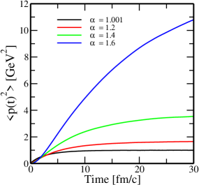
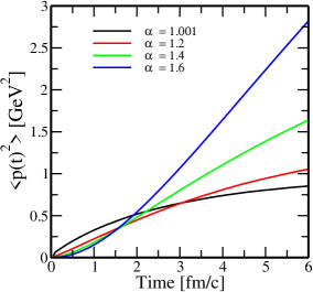
Figure 2: $\langle p^{2}(t)\rangle$ versus time, for the various values of the $\alpha$ and $\mathcal{D}=0.1$ GeV²/fm at $T=250$ MeV.

III Results

III.1 A check for non-relativistic

To analyze the numerical scheme of FLE, we compute $\langle x^{2}(t)\rangle$ from Eq. (24) and $\langle p^{2}(t)\rangle$ from Eq. (25), subsequently comparing the results with the analytical solutions derived from Eq. (20) and Eq. (19), respectively. The FLE has been solved for the 1-D motion of the heavy particle within the nonrelativistic limit, as explained in Sec. II. For illustrative purposes, we have considered constant diffusion coefficient, $\mathcal{D}$ = 0.1 GeV²/fm and mass of the heavy particle, $M$ = 1 GeV and $\gamma=0$ (i.e., pure diffusion case) in FLE. In the left panel of Fig. 1, the numerically computed $\langle p^{2}(t)\rangle$ for $\alpha=1.001$ (brown dashed line), $\alpha=1.2$ (grey dashed line), $\alpha=1.4$ (red dashed line), and $\alpha=1.6$ (orange dashed line) is presented. Notably, these numerical results align with the analytic solutions from Eq. (19) and match the other values of the $\alpha$. For an additional test of our numerical approach, we have calculated $\langle x^{2}(t)\rangle$ of the heavy particle as shown in Fig. 1 (right panel). In the same figure, the numerically calculated $\langle x^{2}(t)\rangle$ for $\alpha=\beta=1.001$ (brown dashed line) and $\alpha=\beta=1.2$ (grey dashed line), $\alpha=\beta=1.4$ (red dashed line), and $\alpha=\beta=1.6$ (orange dashed line) is displayed. Again, the numerical results match the analytic results from Eq. (20). One can notice that the numerical simulation agrees with the analytical result, indicating that our numerical scheme works correctly.

III.2 The evolution of $\langle p^{2}(t)\rangle$ and $\langle x^{2}(t)\rangle$ of the HQs.

For our analysis, the definition we used for $\langle p^{2}(t)\rangle$ is given by

$$\langle p^{2}(t)\rangle=\langle p_{x}^{2}(t)+p_{y}^{2}(t)\rangle.$$ (26)

We have computed $\langle p^{2}(t)\rangle$ over time for four different values of $\alpha$, namely $\alpha=1.001$ (black line), $\alpha=1.2$ (red line), $\alpha=1.4$ (green line), and $\alpha=1.6$ (blue line) at $T=250$ MeV, $M$ = 1.3 GeV and $\mathcal{D}=0.1$ GeV²/fm correspond to the charm quark. The corresponding results are shown in Fig. 2. In this scenario, the initial momentum is set to be $p_{x}(t_{0})=p_{y}(t_{0})=0$.

From the left panel of Fig. 2, it is evident that as the magnitude of $\alpha$ increases, the behaviour of the process indicates superdiffusion for the charm quark within the hot QCD medium. The impact of superdiffusion becomes more noticeable at higher values of $\alpha$. It is noticeable that as $\alpha\rightarrow 1$, the superdiffusion process converges back to normal diffusion. Additionally, in the later stages, the mean squared momentum $\langle p^{2}(t)\rangle$ tends to approach $3MT$ Moore and Teaney (2005), and also the FLE defined in Eq. (25) simplifies to the standard LE described in Ref. Moore and Teaney (2005); Das et al. (2014); He et al. (2012); Young et al. (2012); Lang et al. (2016). This transition emphasizes the connection between superdiffusive behaviour governed by the FLE and the conventional diffusion process characterized by the standard LE. In the right panel of Fig. 2, we present a subset of the results depicted in the left panel, focusing on the early-time evolution of $\langle p^{2}(t)\rangle$ for four different values of $\alpha$. It is worth noting that in the initial time, the diffusion process gradually evolves for higher values of $\alpha$. However, for times beyond $3$ fm/c, the trend reverses, and larger $\alpha$ corresponds to a faster diffusion, as anticipated in Fig. 2 (left panel).

In Fig. 3, we have calculated the evolution of $\langle x^{2}(t)\rangle$ over time for three values of $\alpha=\beta=1.001,1.2,1.4$, maintaining other parameters consistent with those illustrated in Fig. 2. The initial conditions are set to be $x(t_{0})=y(t_{0})=0$. It can be noticed that both $\alpha=\beta=1.2,1.4$, a distinct shift towards superdiffusion is observed (shown in Fig. 3) as we discussed initially in Eq. (1). The larger values of $\alpha$ and $\beta$ contribute to this notable change in behaviour, underlining the complex dynamics of the system. As $\alpha\rightarrow 1$ and $\beta\rightarrow 1$, the behaviour reflects normal diffusion. In this limit, at a later time, $\langle x^{2}(t)\rangle$ exhibits a proportional relationship with $t$, as described in Moore and Teaney (2005); Svetitsky (1988). This puzzling behaviour of $\langle p^{2}(t)\rangle$ and $\langle x^{2}(t)\rangle$ due to the anomalous diffusion, which was not explained before in the context of the HQ dynamics in a hot QCD medium.

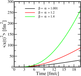
Figure 3: $\langle x^{2}(t)\rangle$ versus time, for the various values of the $\alpha$, $\beta$ and $\mathcal{D}=0.1$ GeV²/fm at $T=250$ MeV.

In the following sections, we have calculated $R_{AA}$ and the charm quark momentum distribution, $dN/dp_{T}$, to see the effect of superdiffusion processes. To determine the interaction of the HQ with the thermalized bath consisting of massless quarks and gluons, we employ perturbative Quantum Chromodynamics (pQCD) transport coefficients for elastic processes with the well-established diffusion coefficients Svetitsky (1988). Here, the Debye mass, $m_{D}=g_{T}T$ screens the infrared divergence associated with the $t$-channel diagrams.

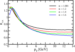
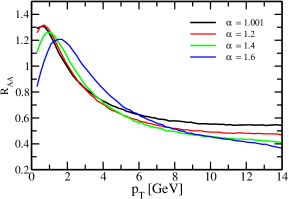
Figure 4: The $R_{AA}$ as a function of $p_{T}$, with $t$ = 6 fm/c, and at two different temperatures ($T$ = 250 MeV (left panel) and $T$ = 350 MeV (right panel) with four different values of $\alpha$.

III.3 Nuclear modification factor

To analyze the impact of the superdiffusion on the experimental observable, we have calculated the nuclear suppression factor, $R_{AA}(p_{T})$ for the HQs, which is defined as follows Moore and Teaney (2005),

$$R_{AA}(p_{T})=\frac{f_{\tau_{f}}(p_{T})}{f_{\tau_{0}}(p_{T})}.$$ (27)

The momentum spectrum, $f_{\tau_{f}}(p)$, of charm quarks calculated for the time evolution, $\tau_{f}$ = $6$ fm/c in our computational results and $f_{\tau_{i}}(p)$ is initial momentum distribution of the charm quark. The initial momentum spectra, $f_{\tau_{i}}(p)$, is taken according to the fixed order + next-to-leading log (FONLL) calculations, which has been shown to be capable of reproducing the spectra of D-mesons produced in proton-proton collisions through fragmentation Cacciari et al. (2005, 2012), the initial momentum spectrum is written as,

$$\frac{dN}{d^{2}p{{}_{T}}}=\frac{x_{0}}{(x_{1}+p_{T})^{x_{2}}},$$ (28)

where the parameters are estimated as follow; $x_{0}=6.365480\times{10}^{8}$, $x_{1}=9.0$ and $x_{2}=10.27890$. $R_{AA}(p_{T})$ $\neq$ 1 implies that charm quarks undergo interactions with the medium. These interactions lead to modifications in the spectrum of charm quarks.

In Fig. 4, the behaviour of $R_{AA}$ is depicted as a function of $p_{T}$, which are calculated using the FLE as defined in Eq. (25) for different values of $\alpha$. The calculations are performed at two distinct temperatures, $T$= 250 MeV (left panel) and $T$= 350 MeV (right panel). At $T$= 250 MeV, the dominating influence is the drag force across the entire range of $p_{T}$. As $p_{T}$ increases, the significance of energy loss becomes more pronounced, which can be noticed in Fig. 4 (left panel). When $\alpha>$ 1, the normal diffusion converts into superdiffusion, it is evident for $\alpha=1.2$ (red line), $\alpha=1.4$ (blue line), and $\alpha=1.6$ (green line). With an increasing value of $\alpha$, there is a notable decrease in magnitude $R_{AA}$ (more suppression) at high $p_{T}$. For $\alpha\rightarrow 1$ (depicted by the black line), the behaviour of the $R_{AA}$ aligns with normal diffusion, consistent with findings available in the literature for the same input parameters Lang et al. (2016); Das et al. (2014, 2015). Fig. 4 (right panel), corresponds to $T=350$ MeV, the observed behaviour is attributed to the diffusion-dominated propagation of the HQs within the hot QCD medium. This dominance of diffusion mechanisms effectively leads to the diffusion of low-momentum charm quarks to higher momentum states. The high temperature, $T=350$ MeV, enhances the significance of diffusion processes, resulting in a distinct pattern in the $R_{AA}$ as compared to $R_{AA}$ at $T$= 250 MeV. For $\alpha>$ 1, a significant reduction in the magnitude of $R_{AA}$ is observed, indicating more suppression at high $p_{T}$. Notably, for the highest considered value of $\alpha=1.6$, a larger proportion of particles tends to remain at low $p_{T}$, a consequence of the superdiffusion process. This behaviour underscores the complex dynamics associated with superdiffusion and its impact on the $R_{AA}$ of the HQs in the QGP medium.

III.4 Momentum spread of HQs

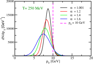
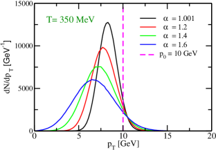
Figure 5: The evolution of charm quark momentum distribution at $\tau_{f}$ = 6 fm/c as a function of $p_{T}$, for various $\alpha$ and at two different temperatures ($T$ = 250 MeV (above panel) and $T$ = 350 MeV (below panel). Assuming an initial delta distribution centered at $p(t_{0})$ = 10 GeV.

We show the evolution of charm momentum distribution, $dN/dp_{T}$, at static temperatures, $T$ = 250 MeV (top panel) and $T$ = 350 MeV (bottom panel) in Fig. 5. The $dN/dp_{T}$ evolution is performed for various values of $\alpha$ at a final evolution time of $\tau_{f}$ = 6 fm/c. To understand the impact of superdiffusion on charm quarks within the QGP, we take initial conditions where all charm quarks are concentrated within an extremely narrow $p_{T}$ bin, creating a delta-like distribution at $p(t_{0})$ = 10 GeV (magenta line). It is observed that the interaction of the HQs with the QGP medium results in the spreading of $dN/dp_{T}$. Subsequently, the evolution of this distribution is analyzed using the FLE as defined in Eq. (25). We have observed the evolution of $dN/dp_{T}$ at higher values of $\alpha$ for the case of superdiffusion, where, $\alpha=1.2$ (red line), $\alpha=1.4$ (blue line), and $\alpha=1.6$ (green line). As depicted in Fig. 5, when $\alpha>1$, the distribution $dN/dp_{T}$ undergoes a notable spread and average momentum shifts towards lower values of $p_{T}$ under the influence of diffusion and drag coefficients, respectively. Specifically, for $\alpha=1.6$ (represented by the blue line), the extent of spreading is more pronounced, and the average momentum shifts towards the lower $p_{T}$ compared to other $\alpha$ values such as 1.001, 1.2, and 1.4. However, for $\alpha$ = 1.001 (black line), corresponding to the normal diffusion coefficient as explained in Ref. Cao and Bass (2011); Das et al. (2014). At the same time, the total area under the curve remains constant for all values of $\alpha$ and both temperatures.

IV Conclusion and outlooks

In this paper, we have discussed anomalous diffusion through the FLE with the Caputo fractional derivative, specifically focusing on superdiffusion in the context of the HQs in the QGP medium. Notably, the mean squared displacement of the particle exhibits a power-law dependence on time (as shown in Fig. 3). Our analysis discussed the scenarios where the values of $\alpha$ and $\beta$ were taken as 1.001, 1.2, 1.4, and 1.6, showcasing the effects of superdiffusion. We have demonstrated that as $\alpha$ approaches 1, the superdiffusion reverts to normal diffusion, verified by numerical and analytical calculations for $\langle x^{2}(t)\rangle$ and $\langle p^{2}(t)\rangle$ in the non-relativistic 1-D case (see Fig. 1). Several key quantities characterizing the dynamics of the HQs under superdiffusion have been computed, including the $\langle p^{2}(t)\rangle$, $\langle x^{2}(t)\rangle$. Extending our analysis, we incorporated physical observables $R_{AA}$ of the HQs in the QGP medium. We then shifted our focus to the momentum spread, $dN/dp_{T}$, utilizing an initial momentum distribution at $p(t_{0})=10$ GeV. The FLE, with the HQs moving under dissipative and random forces, was solved with transport coefficients serving as input parameters. Our findings indicate that superdiffusion results in more suppression in $R_{AA}$. To select specific values for $\alpha$ and $\beta$ within the ranges of $1<\alpha\leq 2$ and $1<\beta\leq 2$, it is essential to be able to simultaneously describe the experimental observables, such as $R_{AA}$ and $v_{2}$, for the entire measured range of $p_{T}$.

In the future, we plan to explore the impact of superdiffusion on the HQ dynamics in the QGP medium, especially considering the time correlation of thermal noise. This study devotes the groundwork for more realistic conditions, which should incorporate an exact initial geometry and an expanding medium in the near future. It is interesting to study the $v_{2}$ of the HQ in the context of superdiffusion within an expanding QGP medium. Superdiffusion might impact various observables, such as HQs directed flow, particle correlations, etc. Given the simplifying assumptions made in our current study, it is challenging to anticipate the specific modifications. A more comprehensive and quantitative analysis will be performed in near future investigations to understand these phenomena further.

V Acknowledgements

I gratefully acknowledge Dr. Santosh Kumar Das for his invaluable advice, Aditi Tomar for insightful discussions and inspirational encouragement, and Mohammad Yousuf Jamal for his numerous informative contributions, collectively enriching the content of this paper. Additionally, I acknowledge the support provided by the BRNS Project No.: 2021/EMR/SKD/026.

VI Appendix

Consider a partition $\{t_{n}=\frac{nT}{N},;0\leq n\leq N\}$ of time interval $[0,T]$. The three-step numerical scheme called L2 approximation is used for the case of superdiffusion. The second derivative $u^{(2)}$ is approximated using a central difference formula, and the resulting numerical scheme involves the values of $u$ at the previous three-time points $u^{n-1}$, $u^{n-2}$, and $u^{n-3}$.

For $1<\nu\leq 2$, superdiffusion

$${}^{C}D^{\nu}_{0+}u(t_{n}) =\frac{1}{\Gamma({2-\nu})}\int_{0}^{t_{n}}\frac{u^{(2)}(s)}{(t_{n}-s)^{\nu-1}}ds$$

$$=\frac{1}{\Gamma({2-\nu})}\sum_{j=1}^{n}\int_{t_{j-1}}^{t_{j}}\frac{u^{(2)}(s)}{(t_{n}-s)^{\nu-1}}ds$$

$$\approx\frac{1}{\Gamma({2-\nu})}\sum_{j=1}^{n}\frac{u(t_{j})-2u(t_{j-1})+u(t_{j-2})}{\Delta t^{2}}\int_{t_{j-1}}^{t_{j}}\frac{1}{(t_{n}-s)^{\nu-1}}ds$$

$$=\frac{1}{\Gamma({3-\nu})}\sum_{j=1}^{n}\frac{((t_{n}-t_{j-1})^{2-\nu}-(t_{n}-t_{j})^{2-\nu})}{\Delta t^{2}}(u(t_{j})-2u(t_{j-1})+u(t_{j-2}))$$

$$=\sum_{j=0}^{n-2}b_{j}(u(t_{n-j})-2u(t_{n-j-1})+u(t_{n-j-2}))$$

$$+\frac{n^{2-\nu}-(n-1)^{2-\nu}}{\Gamma(3-\nu)\Delta t^{\nu}}(u(t_{1})-u(t_{0})).$$ (29)

$$^{C}D^{\nu}_{n}u(t_{n})=\begin{cases}\displaystyle\frac{u^{1}-u^{0}}{\Delta t^{\nu}\Gamma(3-\nu)}\;&:\;n=1\\ \displaystyle\frac{u^{2}-2u^{1}+u^{0}}{\Delta t^{\nu}\Gamma(3-\nu)}\;&:\;n=2\\ \displaystyle\frac{u^{n}-2u^{n-1}+u^{n-2}}{\Delta t^{\nu}\Gamma(3-\nu)}+\sum_{j=1}^{n-2}b_{j}(u^{n-j}-2u^{n-j-1}+u^{n-j-2})&\\ \displaystyle+\;\frac{n^{2-\nu}-(n-1)^{2-\nu}}{\Gamma(3-\nu)\Delta t^{\nu}}(u^{1}-u^{0})\;&:\;n\geq 3\end{cases}$$ (30)

where the coefficients $b_{j}=\frac{(j+1)^{2-\nu}-j^{2-\nu}}{\Gamma(3-\nu)\Delta t^{\nu}}$ in the scheme is determined by the difference formula for the second derivative and are used to account for the fractional order.

References

- Adams et al. (2006) J. Adams et al. (STAR), Phys. Rev. Lett. 97, 162301 (2006), arXiv:nucl-ex/0604018 .
- Adams et al. (2005) J. Adams et al. (STAR), Nucl. Phys. A 757, 102 (2005), arXiv:nucl-ex/0501009 .
- Adcox et al. (2005) K. Adcox et al. (PHENIX), Nucl. Phys. A 757, 184 (2005), arXiv:nucl-ex/0410003 .
- Aamodt et al. (2010) K. Aamodt et al. (ALICE), Phys. Rev. Lett. 105, 252301 (2010), arXiv:1011.3916 [nucl-ex] .
- Arsene et al. (2005) I. Arsene et al. (BRAHMS), Phys. Rev. C 72, 014908 (2005), arXiv:nucl-ex/0503010 .
- van Hees and Rapp (2005) H. van Hees and R. Rapp, Phys. Rev. C 71, 034907 (2005), arXiv:nucl-th/0412015 .
- Rapp and van Hees (2010) R. Rapp and H. van Hees (2010) pp. 111–206, arXiv:0903.1096 [hep-ph] .
- Song et al. (2015) T. Song, H. Berrehrah, D. Cabrera, J. M. Torres-Rincon, L. Tolos, W. Cassing, and E. Bratkovskaya, Phys. Rev. C 92, 014910 (2015), arXiv:1503.03039 [nucl-th] .
- Andronic et al. (2016) A. Andronic et al., Eur. Phys. J. C 76, 107 (2016), arXiv:1506.03981 [nucl-ex] .
- Dong and Greco (2019) X. Dong and V. Greco, Prog. Part. Nucl. Phys. 104, 97 (2019).
- Cao et al. (2019) S. Cao et al., Phys. Rev. C 99, 054907 (2019), arXiv:1809.07894 [nucl-th] .
- Beraudo et al. (2018) A. Beraudo et al., Nucl. Phys. A 979, 21 (2018), arXiv:1803.03824 [nucl-th] .
- Prino and Rapp (2016) F. Prino and R. Rapp, J. Phys. G 43, 093002 (2016), arXiv:1603.00529 [nucl-ex] .
- Aarts et al. (2017) G. Aarts et al., Eur. Phys. J. A 53, 93 (2017), arXiv:1612.08032 [nucl-th] .
- Uphoff et al. (2011) J. Uphoff, O. Fochler, Z. Xu, and C. Greiner, Phys. Rev. C 84, 024908 (2011), arXiv:1104.2295 [hep-ph] .
- Golam Mustafa et al. (1998) M. Golam Mustafa, D. Pal, and D. Kumar Srivastava, Phys. Rev. C 57, 889 (1998), [Erratum: Phys.Rev.C 57, 3499–3499 (1998)], arXiv:nucl-th/9706001 .
- Plumari et al. (2018) S. Plumari, V. Minissale, S. K. Das, G. Coci, and V. Greco, Eur. Phys. J. C 78, 348 (2018), arXiv:1712.00730 [hep-ph] .
- Gossiaux and Aichelin (2008) P. B. Gossiaux and J. Aichelin, Phys. Rev. C 78, 014904 (2008), arXiv:0802.2525 [hep-ph] .
- Prakash et al. (2021) J. Prakash, M. Kurian, S. K. Das, and V. Chandra, Phys. Rev. D 103, 094009 (2021), arXiv:2102.07082 [hep-ph] .
- Prakash et al. (2023) J. Prakash, V. Chandra, and S. K. Das, Phys. Rev. D 108, 096016 (2023), arXiv:2306.07966 [hep-ph] .
- Prakash and Jamal (2023a) J. Prakash and M. Y. Jamal, (2023a), arXiv:2304.04003 [nucl-th] .
- Jamal et al. (2023) M. Y. Jamal, J. Prakash, I. Nilima, and A. Bandyopadhyay, (2023), arXiv:2304.09851 [hep-ph] .
- Singh et al. (2023) M. Singh, M. Kurian, S. Jeon, and C. Gale, Phys. Rev. C 108, 054901 (2023), arXiv:2306.09514 [nucl-th] .
- Kurian et al. (2020) M. Kurian, M. Singh, V. Chandra, S. Jeon, and C. Gale, Phys. Rev. C 102, 044907 (2020), arXiv:2007.07705 [hep-ph] .
- Cao et al. (2016) S. Cao, T. Luo, G.-Y. Qin, and X.-N. Wang, Phys. Rev. C 94, 014909 (2016), arXiv:1605.06447 [nucl-th] .
- Mazumder et al. (2011) S. Mazumder, T. Bhattacharyya, J.-e. Alam, and S. K. Das, Phys. Rev. C 84, 044901 (2011), arXiv:1106.2615 [nucl-th] .
- Zhang et al. (2023) C. Zhang, L. Zheng, S. Shi, and Z.-W. Lin, Phys. Lett. B 846, 138219 (2023), arXiv:2210.07767 [nucl-th] .
- Jamal et al. (2021) M. Y. Jamal, S. K. Das, and M. Ruggieri, Phys. Rev. D 103, 054030 (2021).
- Jamal and Mohanty (2021a) M. Y. Jamal and B. Mohanty, Eur. Phys. J. C 81, 616 (2021a), arXiv:2101.00164 [nucl-th] .
- Jamal and Mohanty (2021b) M. Y. Jamal and B. Mohanty, Eur. Phys. J. Plus 136, 130 (2021b), arXiv:2002.09230 [nucl-th] .
- Sun et al. (2023) Y. Sun, S. Plumari, and S. K. Das, Phys. Lett. B 843, 138043 (2023), arXiv:2304.12792 [nucl-th] .
- Plumari et al. (2020) S. Plumari, G. Coci, V. Minissale, S. K. Das, Y. Sun, and V. Greco, Phys. Lett. B 805, 135460 (2020), arXiv:1912.09350 [hep-ph] .
- Prakash and Jamal (2023b) J. Prakash and M. Y. Jamal, Journal of Physics G: Nuclear and Particle Physics 51, 025101 (2023b).
- Debnath et al. (2023) M. Debnath, R. Ghosh, M. Y. Jamal, M. Kurian, and J. Prakash, (2023), arXiv:2311.16005 [hep-ph] .
- Du and Qian (2023) X. Du and W. Qian, arXiv preprint arXiv:2312.16294 (2023).
- Shaikh et al. (2021) A. Shaikh, M. Kurian, S. K. Das, V. Chandra, S. Dash, and B. K. Nandi, Phys. Rev. D 104, 034017 (2021), arXiv:2105.14296 [hep-ph] .
- Kumar et al. (2022) A. Kumar, M. Kurian, S. K. Das, and V. Chandra, Phys. Rev. C 105, 054903 (2022), arXiv:2111.07563 [hep-ph] .
- Das et al. (2022) S. K. Das et al., International Journal of Modern Physics E , 2250097 (2022).
- Kubo et al. (2012) R. Kubo, M. Toda, and N. Hashitsume, 31 (2012).
- Young et al. (2012) C. Young, B. Schenke, S. Jeon, and C. Gale, Phys. Rev. C 86, 034905 (2012).
- Lang et al. (2016) T. Lang, H. van Hees, G. Inghirami, J. Steinheimer, and M. Bleicher, Phys. Rev. C 93, 014901 (2016).
- Cao and Bass (2011) S. Cao and S. A. Bass, Phys. Rev. C 84, 064902 (2011).
- van Hees et al. (2008) H. van Hees, M. Mannarelli, V. Greco, and R. Rapp, Phys. Rev. Lett. 100, 192301 (2008), arXiv:0709.2884 [hep-ph] .
- Das et al. (2014) S. K. Das, F. Scardina, S. Plumari, and V. Greco, Phys. Rev. C 90, 044901 (2014), arXiv:1312.6857 [nucl-th] .
- He et al. (2023) M. He, H. van Hees, and R. Rapp, Prog. Part. Nucl. Phys. 130, 104020 (2023), arXiv:2204.09299 [hep-ph] .
- He et al. (2012) M. He, R. J. Fries, and R. Rapp, Phys. Rev. C 86, 014903 (2012).
- Das et al. (2015) S. K. Das, F. Scardina, S. Plumari, and V. Greco, Phys. Lett. B 747, 260 (2015), arXiv:1502.03757 [nucl-th] .
- Balescu (1995) R. Balescu, Physical Review E 51, 4807 (1995).
- Bouchaud and Georges (1990) J.-P. Bouchaud and A. Georges, Physics reports 195, 127 (1990).
- Metzler and Klafter (2000) R. Metzler and J. Klafter, Physics reports 339, 1 (2000).
- Caspi et al. (2000) A. Caspi, R. Granek, and M. Elbaum, Phys. Rev. Lett. 85, 5655 (2000).
- Weber et al. (2010) S. C. Weber, A. J. Spakowitz, and J. A. Theriot, Phys. Rev. Lett. 104, 238102 (2010).
- Vitali et al. (2018) S. Vitali, V. Sposini, O. Sliusarenko, P. Paradisi, G. Castellani, and G. Pagnini, Journal of The Royal Society Interface 15, 20180282 (2018).
- Oliveira et al. (2019) F. A. Oliveira, R. M. Ferreira, L. C. Lapas, and M. H. Vainstein, Frontiers in Physics 7, 18 (2019).
- Sokolov and Klafter (2005) I. M. Sokolov and J. Klafter, Chaos: An Interdisciplinary Journal of Nonlinear Science 15 (2005).
- Lutz (2001) E. Lutz, Phys. Rev. E 64, 051106 (2001).
- Lim and Teo (2009) S. Lim and L. Teo, Journal of Statistical Mechanics: Theory and Experiment 2009, P08015 (2009).
- Wang and Chen (2023) X. Wang and Y. Chen, Phys. Rev. E 107, 024105 (2023).
- Li et al. (2012) C. Li, F. Zeng, and F. Liu, Fractional Calculus and Applied Analysis 15, 383 (2012).
- Kobelev and Romanov (2000) V. Kobelev and E. Romanov, Progress of Theoretical Physics Supplement 139, 470 (2000).
- Coffey et al. (2004) W. T. Coffey, Y. P. Kalmykov, and J. T. Waldron, World Scientific Publishing Co., Inc., River Edge, NJ 105 (2004), 10.1142/5343.
- Gorenflo and Mainardi (1997) R. Gorenflo and F. Mainardi, CISM Courses and Lect., 378, 223 (1997).
- Mainardi and Pironi (1996) F. Mainardi and P. Pironi, Extracta Math. 11, 140 (1996).
- Mainardi (1997) F. Mainardi, CISM Courses and Lect., 378, 291 (1997).
- Guo et al. (2013) P. Guo, C. Zeng, C. Li, and Y. Chen, Fractional Calculus and Applied Analysis 16, 123 (2013).
- Li and Zeng (2013) C. Li and F. Zeng, Numerical Functional Analysis and Optimization 34, 149 (2013).
- Miller and Ross (1993) K. S. Miller and B. Ross, John Wiley & Sons, Inc., New York , xvi+366 (1993).
- Carpinteri and Mainardi (2014) A. Carpinteri and F. Mainardi, Fractals and Fractional Calculus in Continuum Mechanics 378 (2014).
- Agrawal (2007) O. P. Agrawal, Journal of Physics A: Mathematical and Theoretical 40, 6287 (2007).
- Feller (1971) W. Feller, John Wiley and Sons (1971).
- Metzler et al. (1999) R. Metzler, E. Barkai, and J. Klafter, Phys. Rev. Lett. 82, 3563 (1999).
- Metzler (2000) R. Metzler, Phys. Rev. E 62, 6233 (2000).
- Zumofen and Klafter (1994) G. Zumofen and J. Klafter, Chemical physics letters 219, 303 (1994).
- Lomholt et al. (2005) M. A. Lomholt, T. Ambjörnsson, and R. Metzler, Phys. Rev. Lett. 95, 260603 (2005).
- Shlesinger et al. (1993) M. F. Shlesinger, G. M. Zaslavsky, and J. Klafter, Nature 363, 31 (1993).
- Wang and Tokuyama (1999) K. Wang and M. Tokuyama, Physica A: Statistical Mechanics and its Applications 265, 341 (1999).
- Wang (1992a) K. Wang, Physical Review A 45, 833 (1992a).
- Porrà et al. (1996) J. M. Porrà, K.-G. Wang, and J. Masoliver, Phys. Rev. E 53, 5872 (1996).
- Wang (1992b) K. G. Wang, Phys. Rev. A 45, 833 (1992b).
- Fa (2006) K. S. Fa, Phys. Rev. E 73, 061104 (2006).
- Siegle et al. (2010) P. Siegle, I. Goychuk, and P. Hänggi, Phys. Rev. Lett. 105, 100602 (2010).
- Chen et al. (2023) W. Chen, C. Greiner, and Z. Xu, Phys. Rev. E 107, 064131 (2023).
- Hammelmann et al. (2019) J. Hammelmann, J. M. Torres-Rincon, J.-B. Rose, M. Greif, and H. Elfner, Phys. Rev. D 99, 076015 (2019).
- Kapusta et al. (2012) J. I. Kapusta, B. Müller, and M. Stephanov, Phys. Rev. C 85, 054906 (2012).
- Ruggieri et al. (2022) M. Ruggieri, Pooja, J. Prakash, and S. K. Das, Phys. Rev. D 106, 034032 (2022), arXiv:2203.06712 [hep-ph] .
- Pooja et al. (2023) Pooja, S. K. Das, V. Greco, and M. Ruggieri, Phys. Rev. D 108, 054026 (2023), arXiv:2306.13749 [hep-ph] .
- Caucal and Mehtar-Tani (2022) P. Caucal and Y. Mehtar-Tani, Phys. Rev. D 106, L051501 (2022), arXiv:2109.12041 [hep-ph] .
- Caputo (1967) M. Caputo, Geophysical Journal International 13, 529 (1967).
- (89) I. Podlubny, Fractional Differential Equations, Aca- demic Press, San Diego, 1999 .
- Sandev et al. (2012) T. Sandev, R. Metzler, and . Tomovski, Fractional Calculus and Applied Analysis 15, 426 (2012).
- Erdélyi et al. (1953) A. Erdélyi, W. Magnus, F. Oberhettinger, and F. Tricomi, Higher transcendental functions 2, 133 (1953).
- Hilfer (2000) R. Hilfer, World Scientific Publishing Co., Inc., River Edge, NJ , viii+463 (2000).
- Rogers (1997) L. C. G. Rogers, Mathematical finance 7, 95 (1997).
- Oldham and Spanier (1974) K. B. Oldham and J. Spanier, Mathematics in Science and Engineering 111 (1974), 2105.14296 .
- Walton and Rafelski (2000) D. B. Walton and J. Rafelski, Phys. Rev. Lett. 84, 31 (2000).
- Moore and Teaney (2005) G. D. Moore and D. Teaney, Phys. Rev. C 71, 064904 (2005), arXiv:hep-ph/0412346 .
- Mazumder et al. (2014) S. Mazumder, T. Bhattacharyya, and J.-e. Alam, Phys. Rev. D 89, 014002 (2014), arXiv:1305.6445 [nucl-th] .
- Svetitsky (1988) B. Svetitsky, Phys. Rev. D 37, 2484 (1988).
- Cacciari et al. (2005) M. Cacciari, P. Nason, and R. Vogt, Phys. Rev. Lett. 95, 122001 (2005), arXiv:hep-ph/0502203 .
- Cacciari et al. (2012) M. Cacciari, S. Frixione, N. Houdeau, M. L. Mangano, P. Nason, and G. Ridolfi, JHEP 10, 137 (2012), arXiv:1205.6344 [hep-ph] .