Towards Efficient Communication Federated Recommendation System via Low-rank Training

Abstract.

In Federated Recommendation (FedRec) systems, communication costs are a critical bottleneck that arises from the need to transmit neural network models between user devices and a central server. Prior approaches to these challenges often lead to issues such as computational overheads, model specificity constraints, and compatibility issues with secure aggregation protocols. In response, we propose a novel framework, called Correlated Low-rank Structure (CoLR), which leverages the concept of adjusting lightweight trainable parameters while keeping most parameters frozen. Our approach substantially reduces communication overheads without introducing additional computational burdens. Critically, our framework remains fully compatible with secure aggregation protocols, including the robust use of Homomorphic Encryption. Our approach resulted in a reduction of up to 93.75% in payload size, with only an approximate 8% decrease in recommendation performance across datasets. Code for reproducing our experiments can be found at https://github.com/NNHieu/CoLR-FedRec.

1. Introduction

In a centralized recommendation system, all user behavior data is collected on a central server for training. However, this method can potentially expose private information that users may be hesitant to share with others. As a result, various regulations such as the General Data Protection Regulation (GDPR)(Voigt and Von dem Bussche, 2017) and the California Consumer Privacy Act (CCPA)(Pardau, 2018) have been implemented to limit the centralized collection of users’ personal data. In response to this challenge, and in light of the increasing prevalence of edge devices, federated recommendation (FedRec) systems have gained significant attention for their ability to uphold user privacy (Ammad-Ud-Din et al., 2019; Lin et al., 2020a; Chai et al., 2020; Lin et al., 2020b; Wang et al., 2021c, b; Wu et al., 2022; Perifanis and Efraimidis, 2022; Liu et al., 2022).

The training of FedRec systems is often in a cross-device setting which involves transferring recommendation models between a central server and numerous edge devices, such as mobile phones, laptops, and PCs. It is increasingly challenging to transfer these models due to the growing model complexity and parameters in modern recommendation systems (Naumov et al., 2019). In addition, clients participating in FedRec systems often exhibit differences in their computational processing speeds and communication bandwidth capabilities, primarily stemming from variations in their hardware and infrastructure (Li et al., 2020a). These discrepancies can give rise to stragglers and decrease the number of participants involved in training, potentially leading to diminished system performance.

Practical FedRec systems require the implementation of mechanisms that reduce the amount of communication costs. Three commonly used approaches to reduce communication costs include (i) reducing the frequency of communication by allowing local updates, (ii) minimizing the size of the message through message compression, and (iii) reducing the server-side communication traffic by restricting the number of participating clients per round (Wang et al., 2021a). Importantly, these three methods are independent and can be combined for enhanced efficiency.

In this study, we address the challenge of communication efficiency in federated recommendations by introducing an alternative to compression methods. Many existing compression methods involve encoding and decoding steps that can introduce significant delays, potentially outweighing the gains achieved in per-bit communication time (Vogels et al., 2019). Another crucial consideration is the compatibility with aggregation protocols. For example, compression techniques that do not align with all-reduce aggregation may yield reduced communication efficiency in systems employing these aggregation techniques (Vogels et al., 2019). This is also necessary for many secure aggregation protocols such as Homomorphic Encryption (HE) (Bonawitz et al., 2017). Moreover, many algorithms assume that clients have the same computational power, but this may induce stragglers due to computational heterogeneity and can increase the runtime of algorithms.

Based on our observation that the update transferred between clients and the central server in FedRec systems has a low-rank bias (Section 4.1), we propose Correlated Low-rank Structure update (CoLR). CoLR increases communication efficiency by adjusting lightweight trainable parameters while keeping most parameters frozen. Under this training scheme, only a small amount of trainable parameters will be shared between the server and clients. Compared with other compression techniques, our methods offer the following benefits. (i) Reduce both up-link and down-link communication cost: CoLR avoid the need of unrolling the low-rank message in the aggregation step by using a correlated projection, (ii) Low computational overheads: Our method enforces a low-rank structure in the local update during the local optimization stage so eliminates the need to perform a compression step. Moreover, CoLR can be integrated into common aggregation methods such as FedAvg and does not require additional computation. (iii) Compatible with secure aggregation protocols: the aggregation step on CoLR can be carried by simple additive operations, this simplicity makes it compatible with strong secure aggregation methods such as HE, (iv) Bandwidth heterogeneity awareness: Allowing adaptive rank for clients based on computational/communication budget.

Our contributions can be summarized as following:

• We propose a novel framework, CoLR, designed to tackle the communication challenge in training FedRec systems.

• We conducted experiments to showcase the effectiveness of CoLR. Notably, even with an update size equates to 6.25% of the baseline model, CoLR demonstrates remarkable efficiency by retaining 93.65% accuracy (in terms of HR) compared to the much larger baseline.

• We show that CoLR is compatible with HE-based FedRec systems and, hence, reinforces the security of the overall recommendation systems. Our framework demonstrates a capability to provide a strong foundation for building a secure and practical recommendation system.

2. Related Work

Federated Recommendation (FedRec) Systems.

In recent years, FedRec systems have risen to prominence as a key area of research in both machine learning and recommendation systems. FCF (Ammad-Ud-Din et al., 2019) and FedRec (Lin et al., 2020a) are the pioneering FL-based methods for collaborative filtering based on matrix factorization. The former is designed for implicit feedback, while the latter is for explicit feedback. To enhance user privacy, FedMF (Chai et al., 2020) applies distributed matrix factorization within the FL framework and introduces the HE technique for securing gradients before they are transmitted to the server. MetaMF (Lin et al., 2020b) is a distributed matrix factorization framework using a meta-network to generate rating prediction models and private item embedding.  (Wu et al., 2022) presents FedPerGNN, where each user maintains a GNN model to incorporate high-order user-item information. FedNCF (Perifanis and Efraimidis, 2022) adapts Neural Collaborative Filtering (NCF) (He et al., 2017) to the federated setting, incorporating neural networks to learn user-item interaction functions and thus enhancing the model’s learning capabilities.

Communication Efficient Federated Recommendation.

Communication efficiency is of the utmost importance in FL (Konečný et al., 2016). Some works explore reducing the entire item latent matrix payload by meta-learning techniques (Lin et al., 2020b; Wang et al., 2021c). For example, MetaMF (Lin et al., 2020b) adopts the meta recommender to deploy smaller models on the client to reduce memory consumption. LightFR (Zhang et al., 2023) proposes a framework to reduce communication costs by exploiting the learning-to-hash technique under federated settings and enjoys both fast online inference and reduced memory consumption.

Low-rank Structured Update

Konečný et al. (2016) propose to enforce every update to local model $\Delta_{u}$ to have a low rank structure by express $\Delta_{u}=A_{u}^{(t)}B_{u}^{(t)}$ where $A_{u}^{(t)}\in\mathbb{R}^{d_{1}\times k}$ and $B_{u}^{(t)}\in\mathbb{R}^{k\times d_{2}}$. In subsequent computation, $A_{u}^{(t)}\in\mathbb{R}^{d\times k}$ is generated randomly and frozen during a local training procedure. In each round, the method generates the matrix $A_{u}^{(t)}$ afresh for each client independently. This approach saves a factor of $d_{1}/k$. They interpret $B_{u}^{(t)}$ as a projection matrix, and $A_{u}^{(t)}$ as a reconstruction matrix. Hyeon-Woo et al. (2022) proposes a method that re-parameterizes weight parameters of layers using low-rank weights followed by the Hadamard product.

$$W=W_{1}\odot W_{2}=\left(X_{1}Y_{1}^{\top}\right)\odot\left(X_{2}Y_{2}^{\top}\right)$$

Given this parameterization, the rank of $W$ is upper bound by $\operatorname{rank}(W_{1})\operatorname{rank}(W_{2})$ which is less constrained than a conventional low-rank parameterization $W=XY^{\top}$. The authors show that FedPara can achieve comparable performance to the original model with 3 to 10 times lower communication costs on various tasks, such as image classification, and natural language processing.

Secure FedRec.

Sending updates directly to the server without implementing privacy-preserving mechanisms can lead to security vulnerabilities. Chai et al. (2020) demonstrated that in the case of the Matrix Factorization (MF) model using the FedAvg learning algorithm, if adversaries gain access to a user’s gradients in two consecutive steps, they can deduce the user’s rating information. Therefore, it is crucial to incorporate privacy-preserving mechanisms for the update parameters transmitted from clients to the server. One approach, as proposed by Chai et al. (2020), involves leveraging HE to encrypt intermediate parameters before transmitting them to the server. This method effectively safeguards user ratings while maintaining recommendation accuracy. However, it introduces significant computational overhead, including encryption and decryption steps on the client side, as well as aggregation on the server side. Approximately 95% of the time consumed by the system is dedicated to server updates, where all computations are carried out on the ciphertext  Chai et al. (2020).

3. Preliminaries

In this section, we present the preliminaries and the setting that the paper is working with. Also, this part will discuss the challenges in applying compression methods.

3.1. Federated Learning for Recommendation

In the typical settings of item-based FedRec systems (Lin et al., 2020a), there are $M$ users and $N$ items where each user $u$ has a private interaction set denoted as $O_{u}=\{(i,r_{iu})\}\subset[N]\times\mathbb{R}$. These users want to jointly build a recommendation system based on local computations without violating participants’ privacy. This scenario naturally aligns with the horizontal federated setting (McMahan et al., 2017), as it allows us to treat each user as an active participant. In this work, we also use the terms user and client interchangeably. The primary goal of such a system is to generate a ranked list of top-K items that a given user has not interacted with and are relevant to the user’s preferences. Mathematically, we can formalize the problem as finding a global model parameterized by $\theta$ that minimizes the following global loss function $\mathcal{L}(\cdot)$:

(1) $$\mathcal{L}(\theta)\triangleq\sum_{u=1}^{M}w_{u}\mathcal{L}_{u}(\bm{\theta})$$

where $\theta$ is the global parameter, $w_{u}$ is the relative weight of user $u$. And $\mathcal{L}_{u}(\theta):=\sum_{(i,r_{ui})\in O_{u}}\ell_{u}(\theta,(i,r_{ui}))$ is the local loss function at user $u$’s device. Here $(i,r_{ui})$ represents a data sample from the user’s private dataset, and $\ell_{u}$ is the loss function defined by the learning algorithm. Setting $w_{u}=N_{u}/N$ where $N_{u}=|O_{u}|$ and $N=\sum_{u=1}^{M}N_{u}$ makes the objective function $\mathcal{L}(\theta)$ equivalent to the empirical risk minimization objective function of the union of all the users’ dataset. Once the global model is learned, it can be used for user prediction tasks.

In terms of learning algorithms, Federated Averaging (FedAvg) (McMahan et al., 2017) is one of the most popular algorithms in FL. FedAvg divides the training process into rounds. At the beginning of the $t$-th round ($t\geq 0$), the server broadcasts the current global model $\theta^{(t)}$ to a subset of users $\mathcal{S}^{(t)}$ which is often uniformly sampled without replacement in simulation (Wang et al., 2021a; Lin et al., 2020a). Then each sampled client in the round’s cohort performs $\tau_{u}$ local SGD updates on its own local dataset and sends the local model changes $\Delta_{u}^{(t)}=\theta_{u}^{(t,\tau_{u})}-\theta^{(t)}$ to the server. Finally, the server performs an aggregation step to update the global model:

(2) $$\theta^{(t+1)}=\theta^{(t)}+\frac{\sum_{u\in\mathcal{S}^{(t)}}w_{u}\Delta_{u}^{(t)}}{\sum_{u\in\mathcal{S}^{(t)}}w_{u}}$$

The above procedure will repeat until the algorithm converges.

3.2. Limitation of current compression methods

Communication is one of the main bottlenecks in FedRec systems and can be a serious constraint for both servers and clients. For example, when stragglers with limited network connections exist, the central server must decide whether to wait for them to finish or perform the aggregation step with only available participants. Conversely, on the client side, sending the model updates back to the server can be challenging, as uplink is typically much slower than downlink. The download and upload bandwidths in a real cross-device FL system are estimated at 0.75MB/s and 0.25MB/s, respectively (Wang et al., 2021a). Although diverse optimization techniques exist to enhance communication efficiency, such methods may not preserve privacy. Moreover, tackling privacy and communication efficiency as separate concerns can result in suboptimal solutions.

Top-K compression

The process of allocating memory for copying the gradient (which can grow to a large size, often in the millions) and then sorting this copied data to identify the top-K threshold during each iteration is costly enough that it negates any potential enhancements in overall training time when applied to real-world systems. As a result, employing these gradient compression methods in their simplest form does not yield the expected improvements in training efficiency. As observed in Gupta et al. (2021), employing the Top-K compression for training large-scale recommendation models takes 11% more time than the baseline with no compression.

SVD compression

After obtaining factorization results $U_{u}$ and $V_{u}$, the aggregation step requires performing decompression and computing $\sum_{u\in\mathcal{S}}\frac{N_{u}}{N}U_{u}V_{u}$ and this sum is not necessarily low-rank so there is no readily reducing cost in the downlink communication without additional compression-decompression step. The need to perform matrix multiplication makes this method incompatible with HE. Moreover, performing SVD decomposition on an encrypted matrix by known schemes remains an open problem.

4. Proposed method

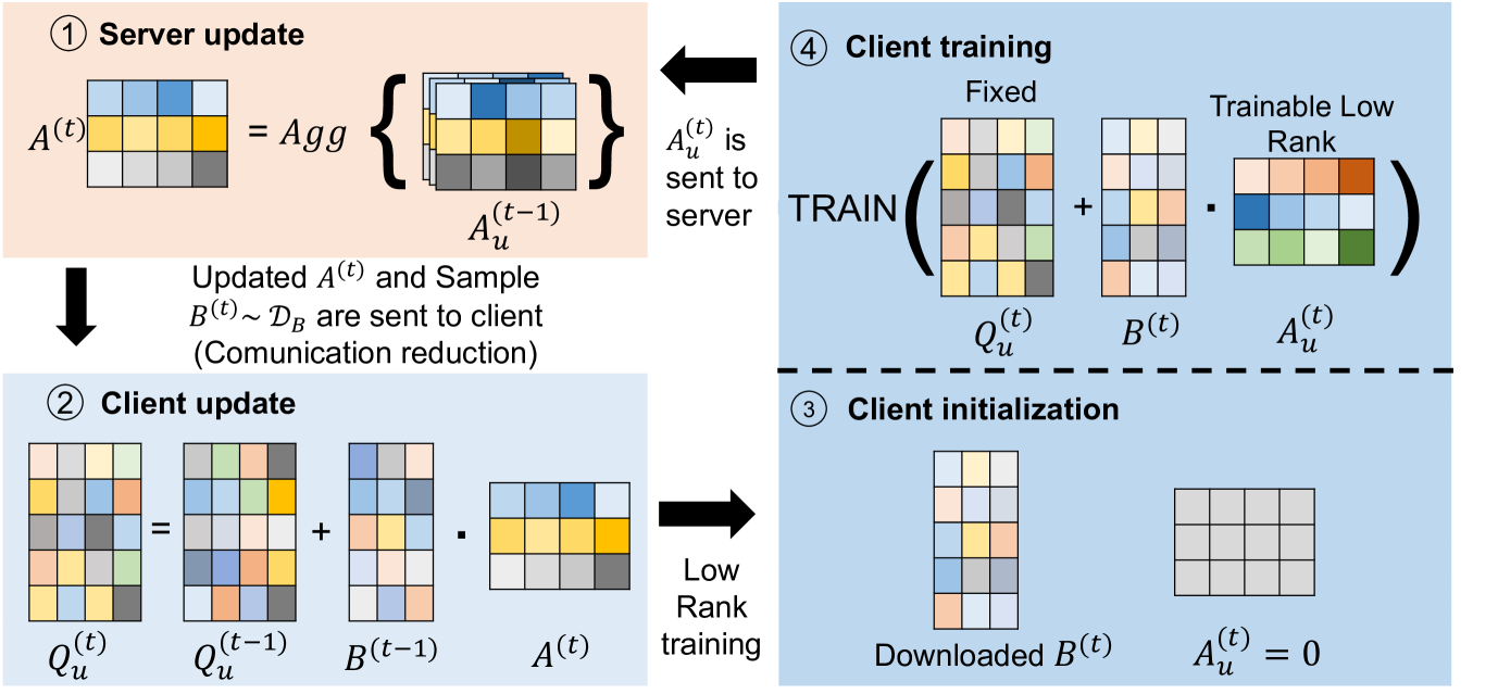
Figure 1. Illustration of CoLR at training round $t$. At first, the server conducts aggregation over the local model $A_{u}^{(t-1,\tau_{u})}$ to obtain the global model update $A^{(t)}$. Subsequently, $A^{(t)}$ are transmitted to the clients. The client will update their $Q_{u}^{(t)}$ using this $A^{(t)}$, then initilizes a new matrix $A_{u}^{(t,0)}$ and download the matrix $B^{(t)}$ which is sampled at the server and shared between clients. Finally, the client carries out local training and then sends the local model update $A_{u}^{(t,\tau_{u})}$ to the server for the next training round.

4.1. Motivation

Our method is motivated by analyzing the optimization process at each user’s local device. We consider an effective federated matrix factorization (FedMF) as the backbone model. This model represents each item and user by a vector with the size of $d$ denoted $\mathbf{q}_{i}$ and $\mathbf{p}_{u}$ respectively. And the predicted ratings $r_{ui}$ are given by $\hat{r}_{ui}=\mathbf{q}_{i}^{\top}\mathbf{p}_{u}$. Then the user-wise local parameter $\theta_{u}$ consists of the user $u$’s embedding $\mathbf{p}_{u}$ and the item embedding matrix $Q$, where $\mathbf{q}_{i}$ is the $i$th column of $Q$. The loss function $\mathcal{L}_{u}$ at user $u$’s device is given in the following.

$$\mathcal{L}_{u}(\mathbf{p}_{u},Q)= \sum_{(i,r_{ui})\in O_{u}}\ell\left(r_{ui},({Q^{\top}\mathbf{p}_{u}})_{i}\right)+\lambda\|\mathbf{p}_{u}\|_{2}+\lambda\|Q\|_{2}$$

Let $\eta$ be the learning rate, the update on the user embedding $\mathbf{p}_{u}$ at each local optimization step is given by:

(3) $$\mathbf{p}_{u}^{(t+1)}= \mathbf{p}_{u}^{(t)}(1-\eta\lambda)+\eta Q^{(t)\top}(\mathbf{r}-\hat{\mathbf{r}}^{(t)}).$$

Let $\mathbf{m}\in\mathbb{R}^{N}$ be a binary vector where $\mathbf{m}_{i}=1$ if $i\in O_{u}$, then the item embedding’s $\mathbf{q}_{i}$ is

(4) $$Q^{(t+1)}=Q^{(t)}-\eta(\lambda Q^{(t)}-\left(\mathbf{m}*(\mathbf{r}_{u}-\hat{\mathbf{r}}_{u})\right)\mathbf{p}_{u}^{(t)\top})$$

The update that is sent to the central server has the following formula,

(5) $$\Delta_{Q}^{(t)}=Q^{(t+1)}-Q^{(t)}=\eta\left[\left(\mathbf{m}*(\mathbf{r}_{u}-\hat{\mathbf{r}}_{u})\right)\mathbf{p}_{u}^{(t)\top}-\lambda Q^{(t)}\right]$$

As we can see from equation 4, since each client only stores the presentation of only one user $\mathbf{p}_{u}$, the update on the item embedding matrix on each user’s device at each local step are just sum of a rank-1 matrix and a regularization component. Given that $\lambda$ is typically small, the low-rank component contributes most to the update $\Delta_{Q}^{(t)}$. And if the direction of $\mathbf{p}_{u}$ does not change much during the local optimization phase, the update $\Delta_{Q}^{(t)}$ can stay low-rank. From this observation, we first assume that the update of the item embedding matrix in training FedRec systems $\Delta_{Q}^{(t)}$ can be well approximated by a low-rank matrix. We empirically verify this assumption by monitoring the effective rank of $\Delta_{Q}^{(t)}$ at each training round for different datasets. The result is plotted in figure 2 where we plot the mean and standard deviation averaged over a set of participants in each round.

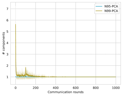
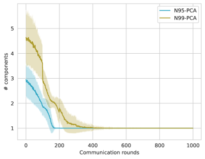
Figure 2. PCA components progression. The figures show the number of components that account for 99% (N99-PCA in green) and 90% (N95-PCA in blue) explained variance of all transfer item embedding matrix across communication rounds on MovieLens-1M (left) and Pinterest (right) datasets.

This analysis suggests that restricting the update to be low-rank can get away with aggressive communication reduction without sacrificing much performance. In the next section, we will propose an efficient communication framework based on this motivation. Since most of the transferred parameters in recommendation models are from the item embedding layers, we will focus on applying the proposed method for embedding layers in this work. Note that our framework can still be applied to different types of layers that are commonly used in recommendation models, such as fully connected layers, convolution layers, and self-attention layers.

4.2. Low-rank Structure

We propose explicitly enforcing a low-rank structure on the local update of the item embedding matrix $Q$. In particular, the local update $(\Delta_{Q})_{u}^{(t)}$ is parameterized by a matrix product

$$(\Delta_{Q})_{u}^{(t)}=B_{u}^{(t)}A_{u}^{(t)}$$

where $B_{u}^{(t)}\in\mathbb{R}^{d\times r}$ and $A_{u}^{(t)}\in\mathbb{R}^{r\times N}$. Given this parameterization, the embedding $\mathbf{q}_{i}$ of an item with index $i$ is given by

$$\mathbf{q}_{i}^{(t)}=\left(Q^{(t)}+B_{u}^{(t)}A_{u}^{(t)}\right)\mathbf{e}_{i}$$

where $\mathbf{e}_{i}\in\mathbb{R}^{N}$ is a one-hot vector whose value at $i$-th is 1. This approach effectively saves a factor of $\frac{N\times d}{N\times r+d\times r}$ in communication since clients only need to send the much smaller matrices $A_{u}$ and $B_{u}$ to the central server.

4.3. Correlated Low-rank Structure Update

Even though enforcing a low-rank structure on the update can greatly reduce the uplink communication size, doing aggregation and performing privacy-preserving is not trivial and faces the following three challenges: (1) the server needs to multiply out all the pairs $A_{u}^{(t)}$ and $B_{u}^{(t)}$ before performing the aggregation step; (2) the sum of low-rank solutions would typically leads to a larger rank update so there is no reducing footprint in the downlink communication; (3) secure aggregation method such as HE cannot directly apply to $A_{u}^{(t)}$ and $B_{u}^{(t)}$ since it will require to perform the multiplication between two encrypted matrices, which is much more costly than simple additive operation.

To reduce the downlink communication cost, we observe that if either $A_{u}^{(t)}$ or $B_{u}^{(t)}$ is identical between users and is fixed during the local training process, then the result of the aggregation step can be represented by a low-rank matrix with the following formulation:

$$\Delta_{Q}^{(t)}=B^{(t)}\left(\sum_{u\in S}A_{u}^{(t)}\right).$$

Notice that this aggregation is also compatible with HE since it only requires additive operations on a set of $A_{u}^{(t)}$ and clients can decrypt this result and then compute the global update $\Delta_{Q}^{(t)}$ at their local device.

Based on the above observation, we propose the Correlated Low-rank Structure Update (CoLR) framework. In this framework, the server randomly initializes a matrix $B^{(t)}$ at the beginning of each training round and shares it among all participants. Participants then set $B_{u}^{(t)}=B^{(t)}$ and freeze this matrix during the local training phase and only optimize for $A_{u}^{(t)}$. The framework is presented in Algorithm 1 and illustrated in Figure 1. Note that the communication cost can be further reduced by sending only the random seed of the matrix $B^{(t)}$. A concurrent work (Anonymous, 2023) proposes FFA-LoRA which also fixes the randomly initialized non-zero matrices and only finetunes the zero-initialized matrices. They study FFA-LoRA in the context of federated fine-tuning LLMs and using differential privacy (Dwork et al., 2006) to provide privacy guarantees.

Input: Initial model $Q^{(0)}$; update rank $r$, a distribution $\mathcal{D}_{B}$ for initializing $B$; ClientOpt, ServerOpt with learning rates $\eta,\eta_{s}$;

1

2for $t\in\{0,1,2,\dots,T\}$  do

3       Sample a subset $\mathcal{S}^{(t)}$ of clients

4       Sample $B^{(t)}\sim\mathcal{D}_{B}$

5       for client $u\in\mathcal{S}^{(t)}$ in parallel do

6             if $t>0$ then

7                   Download $A^{(t)}$

8                   Merge $Q_{u}^{(t,0)}=Q^{(t-1)}+B^{(t-1)}A^{(t)}$

9                  

10             end if

11            Initialize $Q_{u}^{(t,0)}=Q^{(t)}$

12             Download $B^{(t)}$ and Initialize $A_{u}^{(t,0)}=\bm{0}$

13             Set trainable parameters $\theta_{u}^{(t,0)}=\{A_{u}^{(t,0)},\mathbf{p}_{u}^{(t,0)}\}$

14             for $k=0,\dots,\tau_{u}-1$ do

15                  

16                  Compute local stochastic gradient $\nabla\mathcal{L}_{u}(\theta_{u}^{(t,k)})$

17                   Perform local update $\theta_{u}^{(t,k+1)}=\textsc{ClientOpt}\left(\theta_{u}^{(t,k)},\nabla_{\theta_{u}}\mathcal{L}_{u}(\theta_{u}^{(t,k)}),\eta\right)$

18                  

19             end for

20            $\mathbf{p}_{u}^{(t+1)}=\mathbf{p}_{u}^{(t,\tau_{u})}$

21             Upload $\{A_{u}^{(t,\tau_{u})}\}$ to the central server

22            

23       end for

24      Aggregate local changes

$$A^{(t+1)}=\sum_{u\in\mathcal{S}^{(t)}}\dfrac{N_{u}}{N}A_{u}^{(t,\tau_{u})};$$

25 end for

Algorithm 1 Correlated Low-rank Structure Update Matrix Factorization

Differences w.r.t. SVD compression.

We compare our method with SVD since it also uses a low-rank structure. The difference is that in CoLR, participants directly optimize these models on the low-rank parameterization, while SVD only compresses the result from the local training step.

4.4. Subsampling Correlated Low-rank Structure update (SCoLR)

While CoLR offers its merits, there is a potential drawback to consider - it may impact recommendation performance as it confines the global update within a randomly generated low-rank subspace. In the following section, we introduce a modification to this base algorithm, considering a practical reality: downlink bandwidth often surpasses uplink capacity, as observed in cross-device scenarios (Wang et al., 2021a). In these settings, edge devices establish communication with a central server using network connections that vary in quality. Practical implementations have demonstrated significant differences in network bandwidth between download and upload capabilities. We propose a variant of CoLR termed Subsampling Correlated Low-rank Structure update (SCoLR) to address this. SCoLR strategically harnesses the more abundant downlink bandwidth while maintaining communication efficiency and HE compatibility.

We denote $r_{g}$ as the rank of global update, which is sent from the server to participants through downlink connections, and $r_{u}$ as the rank of local update, which is sent from clients to the central server for aggregation through uplink connections. In practice, we can set $r_{g}$ to be larger than $r_{u}$, reflecting that downlink bandwidth is often higher than uplink. Given these rank parameters, at the start of each training round, the central server first initializes a matrix $B$ with the shape of $\mathbb{R}^{d\times r_{g}}$. Then, participants in that round will download this matrix to their local devices and select a subset of columns of $B$ to perform the local optimization step. In particular, we demonstrate this process through the following formulation:

(6) $$(\Delta_{Q})_{u}^{(t)}=BS_{u}A_{u},$$

where $B$ is a matrix with the shape of $\mathbb{R}^{d\times r_{g}}$, $S_{u}$ is a binary matrix with the shape of $\mathbb{R}^{r_{g}\times r_{u}}$ and $A_{u}$ is a matrix with the shape of $\mathbb{R}^{r_{u}\times N}$. Specifically, $S_{u}$ is a binary matrix with $r_{u}$ rows and $r_{g}$ columns, where each row has exactly one non-zero element. The non-zero element in the $i$-th row is at the $j$-th column, where $j$ is the $i$-th element of a randomly shuffled array of integers from 1 to $r_{g}$. The detail is presented in Algorithm 2.

Moreover, in scenarios where clients have diverse computational resources, each can choose a unique local rank, denoted as $r_{u}$, aligning with their specific computational capacities and individual preferences throughout the training process. Importantly, sharing the matrix $S_{u}$ does not divulge sensitive user information. Multiplying this matrix with $S_{u}$ is essentially a row reordering operation on the matrix $A_{u}$. As a result, we can effectively perform additive HE between pairs of rows from $A_{u_{1}}$ and $A_{u_{2}}$. This approach ensures privacy while accommodating varying computational capabilities among clients.

5. Experiments

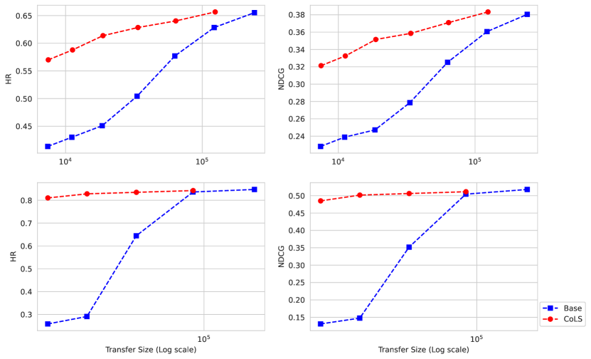
Figure 3. HR and NDCG on MovieLens-1M dataset (Top) and Pinterest Dataset (Bottom). We plot the utilities versus the communication size and compare CoLRwith the base model with the same transfer size. The x-axis is plotted using a log scale.

5.1. Experimental Setup

Table 1. Statistics of the datasets used in evaluation.

Datasets	# Users	# Items	# Ratings	Data Density
MovieLens-1M (Harper and Konstan, 2015)	$6,040$	$3,706$	$1,000,209$	$4.47\%$
Pinterest (Geng et al., 2015)	$55,187$	$9,916$	$1,500,809$	$0.27\%$

Datasets

We experiment with two publicly available datasets, which are MovieLens-1M (Harper and Konstan, 2015) and Pinterest (Geng et al., 2015). Table 1 summarizes the statistics of our datasets. We follow common practice in recommendation systems for preprocessing by retaining users with at least 20 interactions and converting numerical ratings into implicit feedback (Ammad-Ud-Din et al., 2019; He et al., 2017).

Evaluation Protocols

We employ the standard leave-one-out evaluation to set up our test set (He et al., 2017). For each user, we use all their interactions for training while holding out their last interaction for testing. During the testing phase, we randomly sampled 99 non-interacted items for each user and ranked the test item amongst these sampled items.

To evaluate the performance and verify the effectiveness of our model, we utilize two commonly used evaluation metrics, i.e., Hit Ratio (HR) and Normalized Discounted Cumulative Gain (NDCG), which are widely adopted for item ranking tasks. The above two metrics are usually truncated at a particular rank level (e.g. the first $k$ ranked items) to emphasize the importance of the first retrieved items. Intuitively, the HR metric measures whether the test item is present on the top-$k$ ranked list, and the NDCG metric measures the ranking quality, which comprehensively considers both the positions of ratings and the ranking precision.

Models and Optimization.

For the base models, we adopt Matrix Factorization with the FedAvg learning algorithm, also used in Chai et al. (2020). In our experiments, the dimension of user and item embedding $d$ is set to 64 for the MovieLens-1M dataset and 16 for the Pinterest dataset. This is based on our observation that increasing the embedding size on the Pinterest dataset leads to overfitting and decreased performance on the test set. The result is also consistent with (He et al., 2017). We use the simple SGD optimizer for local training at edge devices.

Federated settings.

In each round, we sample $M$ clients uniformly randomly, without replacement in a given round and across rounds. Instead of performing $\tau_{i}$ steps of ClientOpt, we perform $E$ epochs of training over each client’s dataset. This is because, in practical settings, clients have heterogeneous datasets of varying sizes. Thus, specifying a fixed number of steps can cause some clients to repeatedly train on the same examples, while certain clients only see a small fraction of their data.

Baselines.

We compare our framework with two compression methods: SVD and TopK compression. The first method is based on singular value decomposition, which returns a compressed update with a low-rank structure. The second method is based on sparsification, which represents updates as sparse matrices to reduce the transfer size.

Hyper-parameter settings.

To determine hyper-parameters, we create a validation set from the training set by extracting the second last interaction of each user and tuning hyper-parameters on it. We tested the batch size of [32, 64, 128, 256], the learning rate of [0.5, 0.1, 0.05, 0.01], and weight decay in $[5e-4,1e-4]$. For each dataset, we set the number of clients participating in each round to be equal to 1%. The number of aggregation epochs is set at 1000 for MovieLens-1M and 2000 for Pinterest as the training process is converged at these epochs.

Machine

The experiments were conducted on a machine equipped with an Intel(R) Xeon(R) W-1250 CPU @ 3.30GHz and a Quadro RTX 4000 GPU.

5.2. Experimental Results

(1) CoLR can achieve comparable performances with the base models.

Given our primary focus is on recommendation performance within communication-limited environments, we commence our investigation by comparing the recommendation performance between CoLR  and the base model FedMF given the same communication budget. On the ML-1M dataset, we adjust the dimensions of user and item embeddings across the set [1, 2, 4, 8, 16, 32, 64] for FedMF while fixing the embedding size of CoLR  to 64, with different rank settings within [1, 2, 4, 8, 16, 32]. Similarly, for Pinterest, the embedding range for FedMF is [1, 2, 4, 8, 16], while CoLR  has an embedding size of 16 and ranks in the range of [1, 2, 4, 8]. Our settings lead to approximately equivalent transfer sizes for both methods in each dataset.

In Figure 3, we present the HR and NDCG metrics across a range of different transfer sizes. With equal communication budgets, CoLR consistently outperforms their counterparts on both datasets. To illustrate, on the Pinterest dataset, even with an update size equates to 6.25% of the largest model, CoLR achieves a notable performance (81.03% HR and 48.50% NDCG) compared to the base model (84.74% HR and 51.79% NDCG) while attaining a much larger reduction in terms of communication cost (16x). In contrast, the FedMF models with corresponding embedding sizes achieve much lower accuracies. On the MovieLens-1M dataset, we also observe a similar pattern where CoLR consistently demonstrates higher recommendation performance when compared to their counterparts.

The result from this experiment highlights that CoLR can achieve competitive performance when compared to the fully-trained model, FedMF while greatly reducing the cost of communication.

(2) Comparison between CoLR and other compression-based methods.

Table 2. Communication times and Training times for MovieLens-1M dataset.

Method	Communication time (minutes)	Computation time (minutes)	Total Training Time (minutes)
MF-64	80.43	169.07	249.50
CoLR@1	1.26	169.18	170.43
CoLR@2	2.51	169.21	171.72
CoLR@4	5.03	169.27	174.30
CoLR@8	10.05	169.29	179.34
CoLR@16	20.11	169.30	189.41
CoLR@32	40.21	169.38	209.60
SVD@1	1.26	169.49	170.75
SVD@2	2.51	169.50	172.02
SVD@4	5.03	169.53	174.55
SVD@8	10.05	169.59	179.65
SVD@16	20.11	169.64	189.74
SVD@32	40.21	169.60	209.82
TopK@1	2.51	169.76	172.28
TopK@2	5.03	169.79	174.81
TopK@4	10.05	169.82	179.87
TopK@8	20.11	169.92	190.03
TopK@16	40.21	170.14	210.35

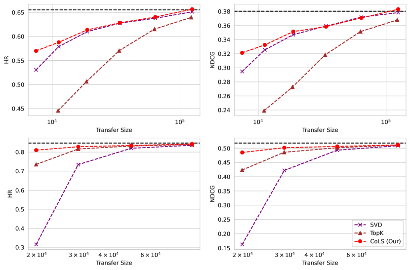
Figure 4. HR and NDCG on MovieLens-1M dataset (Top) and Pinterest Dataset (Bottom). We plot the utilities versus the communication size and compare CoLRwith the base model with the same transfer size. The x-axis is plotted using a log scale. The dashed black line is the base model’s performance with different embedding sizes. For fair comparisons, we set the compression ratio of each method to be equal.

We run the above experiment with two compression methods, SVD and TopK, using equal compression ratios as CoLR. For a fair comparison, we compress both the upload and download messages with the same compression ratio. The result in terms of transfer size is presented in Figure 4. In the case with the same communication budget, CoLR  achieves better performance across the range of communication budgets.

In the previous results, the evaluation of techniques focuses on the overall number of transmitted bits. Although this serves as a broad indicator, it fails to consider the time consumed by encoding/decoding processes and the fixed network latency within the system. When these time delays significantly exceed the per-bit communication time, employing compression techniques may offer limited or minimal benefits. In the following, we do an analysis to understand the effects of using CoLR and compression methods in training FedRec models.

We follow the model from (Wang et al., 2021a) to estimate the communication efficiency of deploying methods to real-world systems. The execution time per round when deploying an optimization algorithm in a cross-device FL system is estimated as follows,

$$T_{\text{round }}(\mathcal{A})=T_{\text{comm }}(\mathcal{A})+T_{\text{comp }}(\mathcal{A}),$$

$$T_{\text{comm }}(\mathcal{A})=\frac{S_{\text{down }}(\mathcal{A})}{B_{\text{down }}}+\frac{S_{\text{up }}(\mathcal{A})}{B_{\text{up }}}$$

$$T_{\text{comp }}(\mathcal{A})=\max_{j\in\mathcal{D}_{\text{round }}}T_{\text{client }}^{j}+T_{\text{server }}(\mathcal{A}),$$

$$T_{\text{client }}^{j}(\mathcal{A})=R_{\text{comp }}T_{\text{sim }}^{j}(\mathcal{A})+C_{\text{comp }}$$

where client download size $S_{\text{d}own}(\mathcal{A})$, upload size $S_{\text{u}p}(\mathcal{A})$, server computation time $T_{\text{server }}$, and client computation time $T_{\text{client }}^{j}$ depend on model and algorithm $\mathcal{A}$. Simulation time $T_{\text{server }}$ and $T_{\text{client }}^{j}$ can be estimated from FL simulation in our machine. We get the estimation of parameters $(B_{\text{down }},B_{\text{up }}),R_{\text{comp }},C_{\text{comp }}$ from Wang et al. (2021a).

$$B_{\text{down }}\sim 0.75\mathrm{MB}/\mathrm{secs},B_{\mathrm{up}}\sim 0.25\mathrm{MB}/\mathrm{secs},$$

$$R_{\mathrm{comp}}\sim 7,\text{ and }C_{\text{comp }}\sim 10\text{ secs. }$$

Table 2 presents our estimation in terms of communication times and computation time. Notice that CoLR adds smaller overheads to the computation time while still greatly reducing the communication cost.

(3) CoLR is compatible with HE

Table 3. Overheads, and Communication ratios for MovieLens-1M dataset; Comm Ratio is calculated by file sizes of Ciphertext over file sizes of Plaintext.

Method	Client overheads	Server overheads	Ciphertext size	Plaintext size	Comm Ratio
FedMF	0.93 s	2.39 s	24,587 KB	927 KB	26.52
FedMF w/ TopK@1/64	88.20 s	88.06 s	3,028 KB	29 KB	103.09
FedMF w/ TopK@2/64	182.02	185.59	6,056 KB	58 KB	103.83
FedMF w/ TopK@4/64	353.25	364.67	12,112 KB	116 KB	104.20
FedMF w/ TopK@8/64	723.45	750.98	24,225 KB	232 KB	104.40
FedMF w/ TopK@16/64	1449.90	1483.91	48,448 KB	464 KB	104.49
FedMF w/ CoLR@1	0.07	0.24	3,073 KB	15 KB	206.31
FedMF w/ CoLR@2	0.07	0.25	3,073 KB	29 KB	104.63
FedMF w/ CoLR@4	0.07	0.25	3,073 KB	58 KB	52.69
FedMF w/ CoLR@8	0.08	0.25	3,073 KB	116 KB	26.44
FedMF w/ CoLR@16	0.15	0.51	6,147 KB	232 KB	26.49
FedMF w/ CoLR@32	0.30	1.03	12,293 KB	464 KB	26.51

In this section, we argue that tackling privacy and communication efficiency as separate concerns can result in suboptimal solutions and point out the limitation in applying SVD and TopK compression on HE-based FedRec systems.

Limitation of HE with SVD Compression: The SVD method necessitates the decomposition of a matrix $M=U*S*V$, requiring matrix multiplication on encrypted matrices U, S, and V derived from local clients’ updates. There are several research endeavors aimed at providing efficient algorithms for applying homomorphic encryption in this context, specifically using the CKKS cryptosystem. However, a limitation of this method is that the dimension of the matrix must be in the form of $2^{n}$, often necessitating additional padding on the original matrices to achieve this form, particularly in the case of larger dimension matrices. Additionally, to reduce the size of global updates sent to the server, additional SVD decompositions are required. Performing SVD decomposition on an encrypted matrix by known schemes remains an open problem, making SVD compression an operation that can result in high bandwidth consumption when transmitting large encrypted matrices in their raw form.

Limitation of HE with TopK Compression: The TopK compression method necessitates in-place homomorphic operations, a characteristic not compatible with the CKKS scheme, designed to perform homomorphic encryption on tensors. As an alternative, we have employed the Paillier cryptosystem, a partially homomorphic encryption scheme capable of encrypting individual numbers. While Paillier allows for the implementation of the FedAvg aggregation strategy for TopK compression, it requires both encryption and decryption operations on local clients, and the secured aggregation process on the server must be executed on each number in the TopK vector. Consequently, increasing the value of K results in higher operational costs for encryption, decryption, and secured aggregation.

In our experiment, we conduct tests using two different compression methods: CoLR and TopK. These tests are carried out under identical configurations, encompassing local updates and the number of clients involved in training rounds. The current setup entails the utilization of the CKKS Cryptosystem for our CoLR method, while the TopK method employs the Paillier cryptosystem for encryption, decryption, and aggregation in place of the TopK vector.

Regarding the runtime aspect, our CoLR compression method leverages the inherent efficiency of the CKKS cryptosystem, which can execute operations on multiple values as a vector. In our approach, for a flattened vector of size $n$, both clients and the server need to perform operations on at most $\lceil\frac{n}{8096}\rceil$ blocks, which incurs minimal computational time. On the other hand, the TopK method necessitates operations to be executed on every value within the TopK vector, leading us to opt for the Paillier cryptosystem as it is partially homomorphic and can accommodate the requirements of both our schemes and the TopK method. In our experimental setup, when the value of $k$ doubles (i.e., doubling the TopK vector’s size), the operation time for both client-side and server-side operations also doubles, as it mandates operations on each value within the vector. Throughout the experiment, our CoLR consistently outperforms the TopK method across various $k$ values, exhibiting lower time overheads on both the client and server sides.

Table 3 shows that CoLR can reduce client and server overheads by up to 10x. When comparing ciphertext to plaintext sizes, the TopK compression method with Paillier encryption demands encryption for each value within the TopK vector. Consequently, whenever the size of the TopK vector doubles, the ciphertext size also doubles. In contrast, as previously explained, our scheme produced at most $\lceil\frac{n}{8096}\rceil$ blocks of ciphertext, with the ciphertext size not doubling each time $k$ doubles. This phenomenon illustrates why, in several cases, the ciphertext size remains consistent even as the plaintext size increases. With higher $k$ values aimed at achieving greater precision, our scheme demonstrates smaller ciphertext sizes, offering a reduction in bandwidth consumption.

5.3. Dynamic local rank

In this section, we evaluate our proposed method SCoLR, where we explore the scenario where each client can dynamically select a random $r_{u}$ value during each training round $t$. This scenario reflects real-world federated learning, where clients often showcase differences in computing capabilities and communication capacities due to hardware discrepancies, as exemplified in (Lai et al., 2021; Li et al., 2020b). It becomes inefficient to impose a uniform training model on all clients within this heterogeneous context, as some devices may not be able to harness their computational resources fully.

For this experiment, we set the global rank $r$ in range $\{4,8,16,32\}$ and uniformly sample the local rank $r_{u}$ such that $1\leq r_{u}\leq r$. It’s crucial to emphasize that $r_{u}$ is independently sampled for each user and may differ from one round to the next. This configuration mirrors a practical scenario where the available resources of a specific user may undergo substantial variations at different time points during the training phase. We present the result on the MovieLens-1M dataset in Table 4. This result demonstrates that SCoLR is effective under the device heterogeneity setting.

Table 4. HR, NDCG of SCoLR algorithm on the MovieLens-1M dataset under computation/device heterogeneity settings.

Global low-rank	Local-rank	HR	NDCG
32	$1-32$	64.59	37.56
16	$1-16$	60.25	34.33
8	$1-8$	52.75	28.41
4	$1-4$	45.99	23.70

6. Conclusion

In this work, we propose Correlated Low-rank Structure update (CoLR), a framework that enhances communication efficiency and privacy preservation in FedRec by leveraging the inherent low-rank structure in updating transfers, our method reduces communication overheads. CoLR also benefits from the CKKS cryptosystem, which allows the implementation of a secured aggregation strategy within FedRec. With minimal computational overheads and bandwidth-heterogeneity awareness, it offers a flexible and efficient means to address the challenges of federated learning. For future research, we see several exciting directions. First, our framework still involves a central server, we would like to test how our methods can be effectively adapted to a fully decentralized, peer-2-peer communication setting. Secondly, investigating methods to handle dynamic network conditions and straggler mitigation in real-world settings will be crucial. Lastly, expanding our approach to accommodate more advanced secure aggregation techniques for reduced server-side computational costs and extending its compatibility with various encryption protocols can further enhance its utility in privacy-sensitive applications.

Appendix A An analysis on the initialization of the matrix B

If each client performs only one GD step locally then $B$ can be seen as the projection matrix and $B\mathbf{a}_{i}$ is the projection of the update of item $i$ on the subspace spanned by columns of $B$. We denoite the error of the update on each item embedding $i$ by $\epsilon_{i}$ which has the following formulation:

(7) $$\epsilon_{i}=\mathbb{E}_{B}\left[\left\|\bar{\Delta}_{Q}-\frac{1}{|S|}\left(\sum_{u\in S}B_{u}\mathbf{a}_{u}\right)\right\|_{2}^{2}\right].$$

We analyze the effect of different initialization of $B$ on this error. First, we state the proposition A.1 which gives an upper bound on the error $\epsilon_{i}$.

Proposition A.1 (Upper bound the error).

If $B_{u}$ is independently generated between users and are chosen from a distribution $\mathcal{B}$ that satisfies:

1. Bounded operator norm: $\mathbb{E}\left[\|B\|^{2}\right]\leq L_{\mathcal{B}}$

2. Bounded bias: $\|\mathbb{E}B_{u}B_{u}^{\top}\bar{\mathbf{p}}_{u}-\bar{\mathbf{p}}_{u}\|_{2}\leq\sqrt{\delta_{\mathcal{B}}}$

Then,

(8) $$\epsilon_{i} =\mathbb{E}_{B}\left[\left\|\bar{\Delta}_{Q}-\frac{1}{|S|}\left(\sum_{u\in S}B_{u}\mathbf{a}_{u}\right)\right\|_{2}^{2}\right]$$

(9) $$\leq\frac{1}{|S|}C_{\mathbf{p}}^{2}\delta_{\mathcal{B}}+\frac{1}{|S|}\max_{u\in S}\alpha_{u}\|\mathbf{p}_{u}\|_{2}^{2}\left(L_{B}^{2}+1\right).$$

Proof.

Assume $B_{u}$ is independently generated between users, we have

$$\epsilon_{i} =\frac{1}{|S|^{2}}\mathbb{E}_{B}\left[\left\|\sum_{u\in S}(r_{ui}-\hat{r}_{ui})\left(B_{u}B_{u}^{\top}\mathbf{p}_{u}-\mathbf{p}_{u}\right)\right\|_{2}^{2}\right]$$

$$=\frac{1}{|S|^{2}}\mathbb{E}_{B}\left[\left\|\sum_{u\in S}\alpha_{u}\left(B_{u}B_{u}^{\top}\mathbf{p}_{u}-\mathbf{p}_{u}\right)\right\|_{2}^{2}\right]$$

$$=\frac{1}{|S|^{2}}\sum_{u_{1}\in S}\sum_{u_{2}\neq u_{1}}\alpha_{u_{1}}\alpha_{u_{2}}\mathbb{E}_{B}\left<B_{u_{1}}B_{u_{1}}^{\top}\mathbf{p}_{u_{1}}-\mathbf{p}_{u_{1}},B_{u_{2}}B_{u_{2}}^{\top}\mathbf{p}_{u_{2}}-\mathbf{p}_{u_{2}}\right>$$

$$+\frac{1}{|S|^{2}}\sum_{u\in S}\alpha^{2}_{u}\mathbb{E}_{B}\left[\left\|B_{u}B_{u}^{\top}\mathbf{p}_{u}-\mathbf{p}_{u}\right\|_{2}^{2}\right]$$

If $B_{u}$ are independently chosen from a distribution $\mathcal{B}$ that satisfies:

1. Bounded operator norm: $\mathbb{E}\left[\|B\|^{2}\right]\leq L_{\mathcal{B}}$

2. Bounded bias: $\|\mathbb{E}B_{u}B_{u}^{\top}\bar{\mathbf{p}}_{u}-\bar{\mathbf{p}}_{u}\|_{2}\leq\sqrt{\delta_{\mathcal{B}}}$

We have

$$\mathbb{E}_{B}\left<B_{u_{1}}B_{u_{1}}^{\top}\mathbf{p}_{u_{1}}-\mathbf{p}_{u_{1}},B_{u_{2}}B_{u_{2}}^{\top}\mathbf{p}_{u_{2}}-\mathbf{p}_{u_{2}}\right>$$

$$=\left\|\mathbf{p}_{u_{1}}\right\|\left\|\mathbf{p}_{u_{2}}\right\|\mathbb{E}_{B}\left<B_{u_{1}}B_{u_{1}}^{\top}\bar{\mathbf{p}}_{u_{1}}-\bar{\mathbf{p}}_{u_{1}},B_{u_{2}}B_{u_{2}}^{\top}\bar{\mathbf{p}}_{u_{2}}-\bar{\mathbf{p}}_{u_{2}}\right>$$

(10) $$=\left\|\mathbf{p}_{u_{1}}\right\|\left\|\mathbf{p}_{u_{2}}\right\|\left<\mathbb{E}B_{u_{1}}B_{u_{1}}^{\top}\bar{\mathbf{p}}_{u_{1}}-\bar{\mathbf{p}}_{u_{1}},\mathbb{E}B_{u_{2}}B_{u_{2}}^{\top}\bar{\mathbf{p}}_{u_{2}}-\bar{\mathbf{p}}_{u_{2}}\right>$$

$$\leq\left\|\mathbf{p}_{u_{1}}\right\|\left\|\mathbf{p}_{u_{2}}\right\|\|\mathbb{E}B_{u_{1}}B_{u_{1}}^{\top}\bar{\mathbf{p}}_{u_{1}}-\bar{\mathbf{p}}_{u_{1}}\|_{2}\|\mathbb{E}B_{u_{2}}B_{u_{2}}^{\top}\bar{\mathbf{p}}_{u_{2}}-\bar{\mathbf{p}}_{u_{2}}\|_{2}$$

(11) $$\leq C_{\mathbf{p}}^{2}\delta_{\mathcal{B}}$$

where (A) follows since $B_{u}$ are independently sampled between users. The second term is

$$\frac{1}{|S|^{2}}\sum_{u\in S}\alpha^{2}_{u}\mathbb{E}_{B}\left[\left\|B_{u}B_{u}^{\top}\mathbf{p}_{u}-\mathbf{p}_{u}\right\|_{2}^{2}\right]$$

$$=\frac{1}{|S|^{2}}\sum_{u\in S}\alpha^{2}_{u}\|\mathbf{p}_{u}\|_{2}^{2}\mathbb{E}_{B}\left[\left\|B_{u}B_{u}^{\top}\bar{\mathbf{p}}_{u}-\bar{\mathbf{p}}_{u}\right\|_{2}^{2}\right]$$

$$=\frac{1}{|S|^{2}}\sum_{u\in S}\alpha_{u}\|\mathbf{p}_{u}\|_{2}^{2}\mathbb{E}_{B}\left[\left\|B_{u}B_{u}^{\top}\bar{\mathbf{p}}_{u}\|_{2}^{2}+\|\bar{\mathbf{p}}_{u}\right\|_{2}^{2}-2\bar{\mathbf{p}}_{u}^{\top}B_{u}B_{u}^{\top}\bar{\mathbf{p}}_{u}\right]$$

$$=\frac{1}{|S|^{2}}\sum_{u\in S}\alpha_{u}\|\mathbf{p}_{u}\|_{2}^{2}\mathbb{E}_{B}\left[\left\|B_{u}B_{u}^{\top}\bar{\mathbf{p}}\right\|_{2}^{2}+1-2\left\|B_{u}^{\top}\bar{\mathbf{p}}\right\|_{2}^{2}\right]$$

$$\leq\frac{1}{|S|}\max_{u\in S}\alpha_{u}\|\mathbf{p}_{u}\|_{2}^{2}\left(\mathbb{E}_{B}\left[\left\|B_{u}B_{u}^{\top}\right\|_{2}^{2}\right]+1\right)$$

$$\leq\frac{1}{|S|}\max_{u\in S}\alpha_{u}\|\mathbf{p}_{u}\|_{2}^{2}\left(L_{B}^{2}+1\right)$$

∎

Next, we bound the bias and the operator norm of $B_{u}$ if it is sampled from a Gaussian distribution in the lemma A.2.

Lemma A.2 (Gaussian Initialization).

Let $r<d$. Consider $B\in\mathbb{R}^{d\times r}$ be sampled from the Gaussian distribution where $B$ has i.i.d. $\mathcal{N}(0,1/k)$ entries and a fixed unit vector $\mathbf{v}\in\mathbf{R}^{d}$. Then

1. Bounded operator norm:

   $$\mathbb{E}\|B\|^{2}\leq\frac{d}{r}\left(1+O\left(\sqrt{\frac{r}{d}}\right)\right)$$

2. Unbias: for every unit vector $\mathbf{v}\in\mathbb{R}^{d}$

   $$\left\|\mathbb{E}BB^{\top}\mathbf{v}-\mathbf{v}\right\|=0$$

Proof.

Let $B^{\prime}=PB$ where $P\in\mathbb{R}^{d\times d}$ is the rotation matrix such that $P\mathbf{v}=\mathbf{e}_{1}$. Due to the rotational symmetry of the normal distribution, $B^{\prime}$ is a random matrix with i.i.d. $\mathcal{N}(0,1/r)$ entries. Note that $B=P^{\top}B^{\prime}$.

$$\mathbb{E}_{B}\left[BB^{\top}\mathbf{v}\right] =\mathbb{E}_{B}\left[P^{\top}PBB^{\top}P^{\top}P\mathbf{v}\right]$$

$$=P^{\top}\mathbb{E}_{B}\left[B^{\prime}B^{\prime\top}\mathbf{e}_{1}\right]$$

Let $\mathbf{z}=B^{\prime}B^{\prime\top}\mathbf{e}_{1}$. Notice that $\mathbf{z}_{j}=\left<B^{\prime\top}\mathbf{e}_{j},B^{\prime\top}\mathbf{e}_{1}\right>$. Because $B^{\prime}$ has i.i.d. $\mathcal{N}(0,1/r)$ entries, $\mathbf{z}_{1}=\|B^{\prime\top}\mathbf{e}_{1}\|_{2}^{2}=\sum_{k=1}^{r}(B^{\prime}_{1k})^{2}$ is $1/r$ times a Chi-square random variable with $r$ degrees of freedom. So $\mathbb{E}[\mathbf{z}_{1}]=\frac{1}{r}r=1$ and $\mathbb{E}[\mathbf{z}_{j}]=0\forall j>1$. Thus, $\mathbb{E}[\mathbf{z}]=\mathbf{e}_{1}$. Therefore, $\left\|\mathbb{E}_{B}\left[BB^{\top}\mathbf{v}\right]\right\|=\left\|P^{\top}\mathbf{e}_{1}-\mathbf{v}\right\|=0.$ ∎

From Proposition A.1 and Lemma A.2, we can directly get the following theorem which bould the error of restricting the local update in a low-rank subspace which is randomly sampled from a normal distribution.

Theorem A.3.

Assume $B_{u}$ is independently generated between users and are chosen from the normal distribution $\mathcal{N}(0,1/r)$. Then,

$$\epsilon_{i} =\mathbb{E}_{B}\left[\left\|\bar{\Delta}_{Q}-\frac{1}{|S|}\left(\sum_{u\in S}B_{u}\mathbf{a}_{u}\right)\right\|_{2}^{2}\right]$$

$$\leq\frac{1}{|S|}\max_{u\in S}\alpha_{u}\|\mathbf{p}_{u}\|_{2}^{2}~{}O\left(\frac{d}{r}\right).$$

This result demonstrates that the square error can increase for lower values of the local rank $r$. Building on this insight, we suggest scaling the learning rate of the low-rank components by $\sqrt{\frac{r}{d}}$ to counter the error.

Experementing with different initialization strategies for $B$

The result in the main text is reported using $B$ sampled from a normal distribution $\mathcal{N}(0,1/r)$. In this section, we experiment with $\mathcal{D}_{B}$ chosen from a normal distribution, distribution of orthonormal matrix, and Gaussian distribution on a unit sphere. The result is s

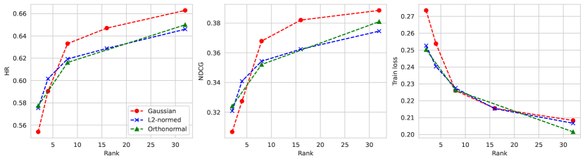
Figure 5. Result with different initialization strategy for $B$ on MovieLens-1M dataset

Appendix B Algorithm Details

In Section 4.4, we presented SCoLR to address the bandwidth heterogeneity problem. We provide the detail of this method in Algorithm 2.

Input: Initial model $Q^{(0)}$; global update rank $r_{g}$, local update rank $\{r_{u}\}$, a distribution $\mathcal{D}_{B}$ for initializing $B$; ClientOpt, ServerOpt with learning rates $\eta,\eta_{s}$;

1

2for $t\in\{0,1,2,\dots,T\}$  do

3       Sample a subset $\mathcal{S}^{(t)}$ of clients

4       Sample $B^{(t)}\sim\mathcal{D}_{B}$

5       for client $u\in\mathcal{S}^{(t)}$ in parallel do

6             if $t>0$ then

7                   Download $A^{(t)}$

8                   Merge $Q_{u}^{(t,0)}=Q^{(t-1)}+B^{(t-1)}A^{(t)}$

9                  

10             end if

11            Initialize $Q_{u}^{(t,0)}=Q^{(t)}$

12             Download $B^{(t)}$, Initialize $A_{u}^{(t,0)}=\bm{0}$, and Randomly sample $S_{u}^{(t)}$

13             Set trainable parameters $\theta_{u}^{(t,0)}=\{A_{u}^{(t,0)},\mathbf{p}_{u}^{(t,0)}\}$

14             for $k=0,\dots,\tau_{u}-1$ do

15                  

16                  Compute local stochastic gradient $\nabla\mathcal{L}_{u}(\theta_{u}^{(t,k)})$

17                   Perform local update $\theta_{u}^{(t,k+1)}=\textsc{ClientOpt}\left(\theta_{u}^{(t,k)},\nabla_{\theta_{u}}\mathcal{L}_{u}(\theta_{u}^{(t,k)}),\eta\right)$

18                  

19             end for

20            $\mathbf{p}_{u}^{(t+1)}=\mathbf{p}_{u}^{(t,\tau_{u})}$

21             Upload $\{S_{u}^{(t)},A_{u}^{(t,\tau_{u})}\}$ to the central server

22            

23       end for

24      Aggregate local changes

$$A^{(t+1)}=\sum_{u\in\mathcal{S}^{(t)}}\dfrac{N_{u}}{N}S_{u}^{(t)}A_{u}^{(t,\tau_{u})};$$

25 end for

Algorithm 2 Subsampling Correlated Low-rank Structure update (SCoLR)

References

- (1)
- Ammad-Ud-Din et al. (2019) Muhammad Ammad-Ud-Din, Elena Ivannikova, Suleiman A Khan, Were Oyomno, Qiang Fu, Kuan Eeik Tan, and Adrian Flanagan. 2019. Federated collaborative filtering for privacy-preserving personalized recommendation system. ArXiv preprint abs/1901.09888 (2019), 4274–4282. https://arxiv.org/abs/1901.09888
- Anonymous (2023) Anonymous. 2023. Improving LoRA in Privacy-preserving Federated Learning. In Submitted to The Twelfth International Conference on Learning Representations. https://openreview.net/forum?id=NLPzL6HWNl under review.
- Bonawitz et al. (2017) Keith Bonawitz, Vladimir Ivanov, Ben Kreuter, Antonio Marcedone, H. Brendan McMahan, Sarvar Patel, Daniel Ramage, Aaron Segal, and Karn Seth. 2017. Practical Secure Aggregation for Privacy-Preserving Machine Learning. In Proceedings of the 2017 ACM SIGSAC Conference on Computer and Communications Security (Dallas, Texas, USA) (CCS ’17). Association for Computing Machinery, New York, NY, USA, 1175–1191. https://doi.org/10.1145/3133956.3133982
- Chai et al. (2020) Di Chai, Leye Wang, Kai Chen, and Qiang Yang. 2020. Secure federated matrix factorization. IEEE Intelligent Systems 36, 5 (2020), 11–20.
- Dwork et al. (2006) Cynthia Dwork, Frank McSherry, Kobbi Nissim, and Adam Smith. 2006. Calibrating Noise to Sensitivity in Private Data Analysis. In Theory of Cryptography, Shai Halevi and Tal Rabin (Eds.). Springer Berlin Heidelberg, Berlin, Heidelberg, 265–284.
- Geng et al. (2015) Xue Geng, Hanwang Zhang, Jingwen Bian, and Tat-Seng Chua. 2015. Learning Image and User Features for Recommendation in Social Networks. In 2015 IEEE International Conference on Computer Vision (ICCV). IEEE Computer Society, 4274–4282. https://doi.org/10.1109/ICCV.2015.486
- Gupta et al. (2021) Vipul Gupta, Dhruv Choudhary, Peter Tang, Xiaohan Wei, Xing Wang, Yuzhen Huang, Arun Kejariwal, Kannan Ramchandran, and Michael W. Mahoney. 2021. Training Recommender Systems at Scale: Communication-Efficient Model and Data Parallelism. In Proceedings of the 27th ACM SIGKDD Conference on Knowledge Discovery & Data Mining (Virtual Event, Singapore) (KDD ’21). Association for Computing Machinery, New York, NY, USA, 2928–2936. https://doi.org/10.1145/3447548.3467080
- Harper and Konstan (2015) F Maxwell Harper and Joseph A Konstan. 2015. The movielens datasets: History and context. ACM Trans. Interact. Intell. Syst. 5, 4 (2015), 1–19.
- He et al. (2017) Xiangnan He, Lizi Liao, Hanwang Zhang, Liqiang Nie, Xia Hu, and Tat-Seng Chua. 2017. Neural Collaborative Filtering. In Proceedings of the 26th International Conference on World Wide Web (Perth, Australia) (WWW ’17). International World Wide Web Conferences Steering Committee, Republic and Canton of Geneva, CHE, 173–182. https://doi.org/10.1145/3038912.3052569
- Hyeon-Woo et al. (2022) Nam Hyeon-Woo, Moon Ye-Bin, and Tae-Hyun Oh. 2022. FedPara: Low-rank Hadamard Product for Communication-Efficient Federated Learning. In International Conference on Learning Representations. OpenReview.net. https://openreview.net/forum?id=d71n4ftoCBy
- Konečný et al. (2016) Jakub Konečný, H. Brendan McMahan, Felix X. Yu, Peter Richtarik, Ananda Theertha Suresh, and Dave Bacon. 2016. Federated Learning: Strategies for Improving Communication Efficiency. In NIPS Workshop on Private Multi-Party Machine Learning. https://arxiv.org/abs/1610.05492
- Lai et al. (2021) Fan Lai, Xiangfeng Zhu, Harsha V. Madhyastha, and Mosharaf Chowdhury. 2021. Oort: Efficient Federated Learning via Guided Participant Selection. In 15th USENIX Symposium on Operating Systems Design and Implementation (OSDI 21). USENIX Association, 19–35. https://www.usenix.org/conference/osdi21/presentation/lai
- Li et al. (2020a) Tian Li, Anit Kumar Sahu, Ameet Talwalkar, and Virginia Smith. 2020a. Federated Learning: Challenges, Methods, and Future Directions. IEEE Signal Processing Magazine 37, 3 (2020), 50–60. https://doi.org/10.1109/MSP.2020.2975749
- Li et al. (2020b) Tian Li, Anit Kumar Sahu, Ameet Talwalkar, and Virginia Smith. 2020b. Federated Learning: Challenges, Methods, and Future Directions. IEEE Signal Processing Magazine 37, 3 (2020), 50–60. https://doi.org/10.1109/MSP.2020.2975749
- Lin et al. (2020a) Guanyu Lin, Feng Liang, Weike Pan, and Zhong Ming. 2020a. Fedrec: Federated recommendation with explicit feedback. IEEE Intell. Syst. 36, 5 (2020), 21–30.
- Lin et al. (2020b) Yujie Lin, Pengjie Ren, Zhumin Chen, Zhaochun Ren, Dongxiao Yu, Jun Ma, Maarten de Rijke, and Xiuzhen Cheng. 2020b. Meta Matrix Factorization for Federated Rating Predictions. In Proceedings of the 43rd International ACM SIGIR Conference on Research and Development in Information Retrieval (Virtual Event, China) (SIGIR ’20). Association for Computing Machinery, New York, NY, USA, 981–990. https://doi.org/10.1145/3397271.3401081
- Liu et al. (2022) Shuchang Liu, Yingqiang Ge, Shuyuan Xu, Yongfeng Zhang, and Amelie Marian. 2022. Fairness-Aware Federated Matrix Factorization. In Proceedings of the 16th ACM Conference on Recommender Systems (Seattle, WA, USA) (RecSys ’22). Association for Computing Machinery, New York, NY, USA, 168–178. https://doi.org/10.1145/3523227.3546771
- McMahan et al. (2017) Brendan McMahan, Eider Moore, Daniel Ramage, Seth Hampson, and Blaise Aguera y Arcas. 2017. Communication-Efficient Learning of Deep Networks from Decentralized Data. In Proceedings of the 20th International Conference on Artificial Intelligence and Statistics (Proceedings of Machine Learning Research, Vol. 54), Aarti Singh and Jerry Zhu (Eds.). PMLR, 1273–1282. https://proceedings.mlr.press/v54/mcmahan17a.html
- Naumov et al. (2019) Maxim Naumov, Dheevatsa Mudigere, Hao-Jun Michael Shi, Jianyu Huang, Narayanan Sundaraman, Jongsoo Park, Xiaodong Wang, Udit Gupta, Carole-Jean Wu, Alisson G. Azzolini, Dmytro Dzhulgakov, Andrey Mallevich, Ilia Cherniavskii, Yinghai Lu, Raghuraman Krishnamoorthi, Ansha Yu, Volodymyr Kondratenko, Stephanie Pereira, Xianjie Chen, Wenlin Chen, Vijay Rao, Bill Jia, Liang Xiong, and Misha Smelyanskiy. 2019. Deep Learning Recommendation Model for Personalization and Recommendation Systems. arXiv:1906.00091 [cs.IR]
- Pardau (2018) Stuart L Pardau. 2018. The California consumer privacy act: Towards a European-style privacy regime in the United States. J. Tech. L. & Pol’y 23 (2018), 68.
- Perifanis and Efraimidis (2022) Vasileios Perifanis and Pavlos S Efraimidis. 2022. Federated Neural Collaborative Filtering. Knowledge-Based Systems 242 (2022), 108441.
- Vogels et al. (2019) Thijs Vogels, Sai Praneeth Karimireddy, and Martin Jaggi. 2019. PowerSGD: Practical Low-Rank Gradient Compression for Distributed Optimization. In Advances in Neural Information Processing Systems, H. Wallach, H. Larochelle, A. Beygelzimer, F. d'Alché-Buc, E. Fox, and R. Garnett (Eds.), Vol. 32. Curran Associates, Inc. https://proceedings.neurips.cc/paper_files/paper/2019/file/d9fbed9da256e344c1fa46bb46c34c5f-Paper.pdf
- Voigt and Von dem Bussche (2017) Paul Voigt and Axel Von dem Bussche. 2017. The eu general data protection regulation (gdpr). A Practical Guide, 1st Ed., Cham: Springer International Publishing 10, 3152676 (2017), 10–5555.
- Wang et al. (2021a) Jianyu Wang, Zachary Burr Charles, Zheng Xu, Gauri Joshi, Brendan McMahan, Blaise Hilary Aguera-Arcas, Maruan Al-Shedivat, Galen Andrew, A. Salman Avestimehr, Katharine Daly, Deepesh Data, Suhas Diggavi, Hubert Eichner, Advait Gadhikar, Zachary Garrett, Antonious M. Girgis, Filip Hanzely, Andrew Hard, Chaoyang He, Samuel Horvath, Zhouyuan Huo, Alex Ingerman, Martin Jaggi, Tara Javidi, Peter Kairouz, Satyen Chandrakant Kale, Sai Praneeth Karimireddy, Jakub Konečný, Sanmi Koyejo, Tian Li, Luyang Liu, Mehryar Mohri, Hang Qi, Sashank Reddi, Peter Richtarik, Karan Singhal, Virginia Smith, Mahdi Soltanolkotabi, Weikang Song, Ananda Theertha Suresh, Sebastian Stich, Ameet Talwalkar, Hongyi Wang, Blake Woodworth, Shanshan Wu, Felix Yu, Honglin Yuan, Manzil Zaheer, Mi Zhang, Tong Zhang, Chunxiang (Jake) Zheng, Chen Zhu, and Wennan Zhu. 2021a. A Field Guide to Federated Optimization. https://arxiv.org/abs/2107.06917
- Wang et al. (2021b) Li-e Wang, Yihui Wang, Yan Bai, Peng Liu, and Xianxian Li. 2021b. POI Recommendation with Federated Learning and Privacy Preserving in Cross Domain Recommendation. In IEEE INFOCOM 2021 - IEEE Conference on Computer Communications Workshops (INFOCOM WKSHPS). 1–6. https://doi.org/10.1109/INFOCOMWKSHPS51825.2021.9484510
- Wang et al. (2021c) Qinyong Wang, Hongzhi Yin, Tong Chen, Junliang Yu, Alexander Zhou, and Xiangliang Zhang. 2021c. Fast-adapting and privacy-preserving federated recommender system. The VLDB Journal (2021), 1–20.
- Wu et al. (2022) Chuhan Wu, Fangzhao Wu, Lingjuan Lyu, Tao Qi, Yongfeng Huang, and Xing Xie. 2022. A federated graph neural network framework for privacy-preserving personalization. Nature Communications 13, 1 (2022), 1–10.
- Zhang et al. (2023) Honglei Zhang, Fangyuan Luo, Jun Wu, Xiangnan He, and Yidong Li. 2023. LightFR: Lightweight Federated Recommendation with Privacy-Preserving Matrix Factorization. ACM Trans. Inf. Syst. 41, 4, Article 90 (mar 2023), 28 pages. https://doi.org/10.1145/3578361