UAV-enabled Integrated Sensing and Communication: Tracking Design and Optimization

Abstract

Integrated sensing and communications (ISAC) enabled by unmanned aerial vehicles (UAVs) is a promising technology to facilitate target tracking applications. In contrast to conventional UAV-based ISAC system designs that mainly focus on estimating the target position, the target velocity estimation also needs to be considered due to its crucial impacts on link maintenance and real-time response, which requires new designs on resource allocation and tracking scheme. In this paper, we propose an extended Kalman filtering-based tracking scheme for a UAV-enabled ISAC system where a UAV tracks a moving object and also communicates with a device attached to the object. Specifically, a weighted sum of predicted posterior Cramér-Rao bound (PCRB) for object relative position and velocity estimation is minimized by optimizing the UAV trajectory, where an efficient solution is obtained based on the successive convex approximation method. Furthermore, under a special case with the measurement mean square error (MSE), the optimal relative motion state is obtained and proved to keep a fixed elevation angle and zero relative velocity. Numerical results validate that the obtained solution to the predicted PCRB minimization can be approximated by the optimal relative motion state when predicted measurement MSE dominates the predicted PCRBs, as well as the effectiveness of the proposed tracking scheme. Moreover, three interesting trade-offs on system performance resulted from the fixed elevation angle are illustrated.

I Introduction

Integrated sensing and communications (ISAC) is expected to merge enhanced sensing services with conventional communication functionalities, including target detection, localization, and tracking [1, 2]. Existing target tracking services in ISAC systems are mainly provided by fixed-position terrestrial ISAC base stations (BSs) [3]. However, the sensing performance of terrestrial ISAC BSs is limited by the constrained coverage area and the unfavorable channel conditions, such as blockage and non-line-of-sight (LoS) links. To overcome these challenges, the unmanned aerial vehicle (UAV)-enabled ISAC has received rapidly increasing research interests thanks to the high maneuverability of UAVs and high probabilities of providing LoS links [4].

Currently, some existing works on UAV-enabled tracking systems investigated the designs for maximizing overall system performance, especially trajectory designs of UAV BSs [5, 6]. In [5], the trajectory of a UAV BS simultaneously communicating with a legitimate user and tracking an eavesdropper was designed to maximize the achievable secrecy rate of the user. In [6], the trajectories of multiple UAVs tracking a ground moving user were jointly designed with the UAV-user association to simultaneously maximize the data rate and minimize the predicted posterior Cramér-Rao bound (PCRB) for the estimated user position, which is constituted by the elements of the state prediction mean square error (MSE) matrix and the predicted measurement MSE matrix. However, neither of the two aforementioned works considered the predicted PCRB for velocity estimation, which has crucial impacts on the link maintenance (e.g., beam alignment) and system responding speed [1]. In fact, most existing ISAC schemes that only focus on estimating the target position are not feasible for highly-reliable target tracking, which thus motivates our new designs on maximizing the sensing performance for both the position and velocity estimation for UAV-enabled ISAC systems.

In this paper, an extended Kalman filtering (EKF)-based tracking scheme is proposed for a UAV-enabled ISAC system, where a UAV tracks a ground moving object to communicate with a device carried by the object. Different from existing works which considered the predicted PCRB for position estimation only, our proposed tracking scheme minimizes a weighted sum of predicted PCRBs for both the estimated position and the estimated velocity by optimizing the predicted state variables (i.e., the relative position and the relative velocity), which is equivalent to the UAV trajectory optimization. This thus generalizes the previous works on UAV-enabled ISAC system designs. The main contributions of this paper are summarized as follows: 1) An efficient solution is obtained based on the successive convex approximation (SCA) method to optimize the predicted state variables for the weighted sum-predicted PCRB minimization. 2) Under a special case where the state prediction MSE matrix is ignored, the optimal relative motion state is obtained and proved to maintain a fixed elevation angle and zero relative velocity between the UAV and the object. 3) Simulation results verify that when the predicted measurement MSE dominates the predicted PCRBs, the obtained solution for the weighted sum-predicted PCRB minimization can be approximated by the optimal relative motion state obtained under the considered special case, and further illustrate three interesting trade-offs achieved by the fixed elevation angle.

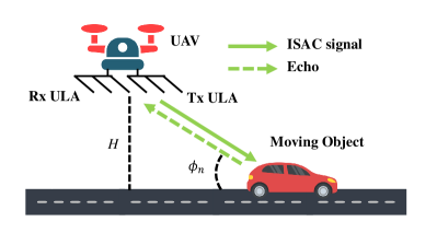
Figure 1: A UAV-enabled ISAC system.

II System Model and Problem Formulation

As illustrated in Fig.1, we consider a downlink UAV-enabled ISAC system, where a UAV simultaneously tracks a moving object and communicates with a single-antenna device attached to the moving object within a service duration $T$. Specifically, the whole service duration $T$ is discretized into $N$ small time slots with a constant length of $\Delta T=T/N$. Let $n$, $n\in\mathbb{N}=\{1,2,...,N\}$, denote the index of time slots. At each time slot, we assume that the motion states (i.e., the position and the velocity) of both the moving object and the UAV keep constant [3]. Therefore, at the $n$th time slot, the object motion state relative to the UAV can be represented by state variables $\mathbf{x}_{n}=[x_{n},v_{n}]^{T}$, where $x_{n}$ and $v_{n}$ denote the relative position and the relative velocity, respectively. In addition, the UAV is equipped with a uniform linear array (ULA) with $N_{t}$ transmit antennas along the $x$-axis and a parallel ULA with $N_{r}$ receive antennas. For ease of analysis, we assume that the object moves along a horizontal straight path parallel to the $x$-axis, and the UAV also flies horizontally along the $x$-axis with a constant altitude $H$.

II-A EKF-based Tracking Scheme

In our proposed tracking scheme, the UAV estimates state variables and designs its next time slot’s trajectory at each time slot. Specifically, we assume that the object movement follows the constant-velocity model [2], and thus the state evolution model can be derived from the geometry as illustrated in Fig.1, which is given by

$$\mathbf{x}_{n}=\mathbf{G}\mathbf{x}_{n-1}-\mathbf{u}_{A,n}+\mathbf{z}_{s,n},\vspace{-1.5mm}$$ (1)

where $\mathbf{G}$ denotes the transition matrix, $\mathbf{u}_{A,n}=[(v_{A,n}-v_{A,n-1})\Delta T,(v_{A,n}-v_{A,n-1})]^{T}$ denotes the increment of the UAV motion state, $v_{A,n}$ denotes the UAV velocity and $\mathbf{z}_{s,n}$ denotes the zero-mean Gaussian distributed process noise with the covariance matrix $\mathbf{Q}_{s}$ at the $n$th time slot. In (1), the expressions of the transition matrix $\mathbf{G}$ and the process noise covariance matrix $\mathbf{Q}_{s}$ can be given by

$$\mathbf{G}=\begin{bmatrix}1&\Delta T\\ 0&1\end{bmatrix},\mathbf{Q}_{s}=\begin{bmatrix}\frac{1}{3}\Delta T^{3}&\frac{1}{2}\Delta T^{2}\\ \frac{1}{2}\Delta T^{2}&\Delta T\end{bmatrix}\tilde{q},\vspace{-1.5mm}$$ (2)

respectively, where $\tilde{q}$ is the process noise intensity [2]. Given the state evolution model, the UAV obtains the estimated state variables for the $n$th time slot given by $\hat{\mathbf{x}}_{n}=\breve{\mathbf{x}}_{n}+\mathbf{K}_{n}(\mathbf{y}_{n}-\mathbf{h}(\breve{\mathbf{x}}_{n}))$, where $\breve{\mathbf{x}}_{n}$ denotes the predicted state variables obtained by $\breve{\mathbf{x}}_{n}=\mathbf{G}\hat{\mathbf{x}}_{n-1}-\mathbf{u}_{A,n}=[\breve{x}_{n},\breve{v}_{n}]^{T}$, $\mathbf{K}_{n}$ denotes the Kalman gain matrix given by $\mathbf{K}_{n}=\mathbf{M}_{p,n}\mathbf{H}_{n}^{H}(\mathbf{Q}_{m,n}+\mathbf{H}_{n}\mathbf{M}_{p,n}\mathbf{H}_{n}^{H})^{-1}$, $\mathbf{M}_{p,n}=\mathbf{G}\mathbf{M}_{n-1}\mathbf{G}^{H}+\mathbf{Q}_{s}$ denotes the state prediction MSE matrix, $\mathbf{M}_{n-1}$ denotes the estimation MSE matrix at the $(n-1)$th time slot, $\mathbf{y}_{n}$, $\mathbf{h}(\cdot)$, $\mathbf{H}_{n}$ and $\mathbf{Q}_{m,n}$ denote the measurement variables, the measurement model, the Jacobian matrix for $\mathbf{h}(\cdot)$ and the measurement noise covariance matrix at the $n$th time slot, respectively, which will be specified in the following subsection.

II-B Signal Model

II-B1 Radar Signal Model

Let $s_{n}(t)\in\mathbb{C}$ denote the information-bearing signal transmitted to the device at time $t$ in the $n$th time slot. Then, the transmitted ISAC signal can be denoted by $\mathbf{s}_{n}(t)=\mathbf{f}_{n}s_{n}(t)$ where $\mathbf{f}_{n}\in\mathbb{C}^{N_{t}\times 1}$ denotes the transmit beamforming vector in the $n$th time slot. The object is modelled as a point scatterer with its radar cross section $\varepsilon$ following a Swerling-I target model [2, 3]. Since the UAV-object channel is dominated by the direct LoS link [4], the large-scale radar channel gain follows a free-space path-loss model: $G_{r,n}=\beta_{r}/d_{n}^{4}$, where $d_{n}$ is the Euclidean distance between the object and the UAV, and the coefficient $\beta_{r}$ is defined as $\beta_{r}\triangleq\lambda^{2}\varepsilon/(64\pi^{3})$ with the carrier wavelength denoted by $\lambda$ [7]. Let $\tau_{n}$ and $\phi_{n}$ denote the round-trip time delay and the elevation angle of the geographical path connecting the UAV to the object at the $n$th time slot, respectively. Thus, the radar channel can be expressed as $\mathbf{h}^{R}_{n}=\sqrt{G_{r,n}}e^{-j4\pi\frac{d_{n}}{\lambda}}\mathbf{b}(\phi_{n})\mathbf{a}^{H}(\phi_{n})$, where $\mathbf{a}(\phi)=[e^{j\frac{\pi(N_{t}-1)\cos{\phi}}{2}},...,e^{-j\frac{\pi(N_{t}-1)\cos{\phi}}{2}}]^{T}$ and $\mathbf{b}(\phi)=[e^{j\frac{\pi(N_{r}-1)\cos{\phi}}{2}},...,e^{-j\frac{\pi(N_{r}-1)\cos{\phi}}{2}}]^{T}$. The reflected echo signals received at the UAV can be given in the form $\mathbf{r}_{n}(t)=\sqrt{P_{A}}\mathbf{h}^{R}_{n}e^{j2\pi\mu_{n}t}\mathbf{f}_{n}s_{n}(t-\tau_{n})+\mathbf{z}_{r,n}(t)$, where $P_{A}$ is the transmit power, $\mu_{n}$ is the Doppler shift and $\mathbf{z}_{r,n}(t)\in\mathbb{C}^{N_{r}\times 1}$ denotes the complex additive white Gaussian noise with zero mean and variance of $\sigma^{2}$.

II-B2 Radar Measurement Model

At the $n$th time slot, the measurement variables are given by $\mathbf{y}_{n}=[\hat{\phi}_{n},\hat{\tau}_{n},\hat{\mu}_{n}]^{T}$, where $\hat{\phi}_{n}$, $\hat{\tau}_{n}$ and $\hat{\mu}_{n}$ denote the measured elevation angle, time delay and Doppler shift, respectively. Specifically, the measured elevation angle $\hat{\phi}_{n}$ can be obtained via the maximum likelihood estimation [8], and then the measured time delay $\hat{\tau}_{n}$ and the measured Doppler frequency $\hat{\mu}_{n}$ can be obtained by performing the standard matched-filtering, which are further expressed as [3]

$$\left\{\begin{aligned} \hat{\phi}_{n}&=\arctan{(H/x_{n})}+z_{\phi,n},\\ \hat{\tau}_{n}&=2(x_{n}^{2}+H^{2})^{\frac{1}{2}}/c+z_{\tau,n},\\ \hat{\mu}_{n}&=2f_{c}v_{n}x_{n}/(c(x_{n}^{2}+H^{2})^{\frac{1}{2}})+z_{\mu,n},\end{aligned}\right.\vspace{-1.5mm}$$ (3)

where $c$ is the speed of light, $z_{\phi,n}\sim\mathbf{\mathcal{N}}\left(0,\sigma_{1,n}^{2}\right)$, $z_{\tau,n}\sim\mathbf{\mathcal{N}}\left(0,\sigma_{2,n}^{2}\right)$ and $z_{\mu,n}\sim\mathbf{\mathcal{N}}\left(0,\sigma_{3,n}^{2}\right)$ denote the measurement noise for the elevation angle, the time delay and the Doppler frequency, respectively. Further, the corresponding measurement noise variance $\sigma_{1,n}^{2}$, $\sigma_{2,n}^{2}$ and $\sigma_{3,n}^{2}$ can be modelled by

$$\left\{\begin{aligned} \sigma_{1,n}^{2}&=(a_{1}^{2}\sigma^{2})/(P_{A}N_{sym}N_{t}N_{r}G_{r,n}\sin^{2}{\phi_{n}}),\\ \sigma_{i,n}^{2}&=(a_{i}^{2}\sigma^{2})/(P_{A}N_{sym}N_{t}N_{r}G_{r,n}),i=2,3,\end{aligned}\right.\vspace{-1.5mm}$$ (4)

where $N_{sym}$ is the number of symbols received during each time slot, and $a_{i},i=1,2,3$ each denotes a constant parameter related to the system configuration [3]. Given (3) and (4), the radar measurement model can thus be compactly formulated as $\mathbf{y}_{n}=\mathbf{h}(\mathbf{x}_{n})+\mathbf{z}_{m,n}$, where $\mathbf{h}(\cdot)$ is defined in (3) and $\mathbf{z}_{m,n}=[z_{\phi,n},z_{\tau,n},z_{\mu,n}]^{T}$ denotes the measurement noise vector with its covariance matrix given by $\mathbf{Q}_{m,n}=\mathrm{diag}(\sigma_{1,n}^{2},\sigma_{2,n}^{2},\sigma_{3,n}^{2})$. Moreover, the Jacobian matrix for $\mathbf{h}(\cdot)$ can be given by

$$\mathbf{H}_{n}=\begin{bmatrix}\iota(\breve{x}_{n})&\kappa(\breve{x}_{n})&\zeta(\breve{x}_{n},\breve{v}_{n})\\ 0&0&\nu(\breve{x}_{n})\end{bmatrix}^{T},\vspace{-1.5mm}$$ (5)

where the expressions of $\iota(\breve{x}_{n})$, $\kappa(\breve{x}_{n})$, $\zeta(\breve{x}_{n},\breve{v}_{n})$ and $\nu(\breve{x}_{n})$ are given in (8), respectively.

II-B3 Communication Signal Model

At the $n$th time slot, the downlink LoS channel between the UAV and the device can be expressed as [7] $\mathbf{h}^{C}_{n}=\sqrt{G_{c,n}}e^{-j2\pi\frac{d_{n}}{\lambda}}\mathbf{a}^{H}(\phi_{n})$, where $G_{c,n}=\lambda^{2}/(16\pi^{2}d_{n}^{2})$ is the large-scale channel power gain. Then, the ISAC signal received by the device at the $n$th time slot can be represented by $c_{n}(t)=\sqrt{P_{A}}\mathbf{h}^{C}_{n}e^{j2\pi\varrho_{n}t}\mathbf{f}_{n}s_{n}(t-\tau_{n})+z_{c}(t)$, where $\varrho_{n}$ denotes the Doppler shift observed at the object, and $z_{c}(t)\sim\mathbf{\mathcal{N}}\left(0,\sigma_{C}^{2}\right)$ is the additive Gaussian noise. Therefore, the achievable date rate can be denoted by $R_{n}=\mathrm{log}_{2}(1+\mathrm{SNR}_{n}^{C})$, where $\mathrm{SNR}_{n}^{C}=P_{A}N_{t}G_{c,n}/\sigma_{C}^{2}$ is the receive signal-to-noise ratio (SNR) of the device.

II-C Problem Formulation

In our proposed tracking scheme, the sensing performance is characterized by the weighted sum of predicted PCRBs for state variables [3, 2]. Specifically, for EKF-based state estimation, the predicted PCRBs for state variables can be denoted by $\breve{\mathrm{PCRB}}_{x,n}=[\breve{\mathbf{M}}_{n}]_{11}=\frac{A_{n}(\breve{x}_{n})}{L_{n}(\breve{x}_{n},\breve{v}_{n})}$ and $\breve{\mathrm{PCRB}}_{v,n}=[\breve{\mathbf{M}}_{n}]_{22}=\frac{B_{n}(\breve{x}_{n},\breve{v}_{n})}{L_{n}(\breve{x}_{n},\breve{v}_{n})}$, respectively, where the expressions of $A_{n}(\breve{x}_{n})$, $B_{n}(\breve{x}_{n},\breve{v}_{n})$, $L_{n}(\breve{x}_{n},\breve{v}_{n})$ are given by (9)-(10), $\breve{\mathbf{M}}_{n}$ denotes the predicted MSE matrix at the $n$th time slot given by [9] $\breve{\mathbf{M}}_{n}=(\breve{\mathbf{M}}_{m,n}^{-1}+\mathbf{M}_{p,n}^{-1})^{-1}$, where $\breve{\mathbf{M}}_{m,n}=(\mathbf{H}_{n}^{H}\breve{\mathbf{Q}}_{m,n}^{-1}\mathbf{H}_{n})^{-1}$ denotes the predicted measurement MSE matrix and $\breve{\mathbf{Q}}_{m,n}=\mathrm{diag}(\breve{\sigma}_{1,n}^{2}(\breve{x}_{n}),\breve{\sigma}_{2,n}^{2}(\breve{x}_{n}),\breve{\sigma}_{3,n}^{2}(\breve{x}_{n}))$ denotes the predicted measurement noise covariance matrix. The expressions of $\breve{\sigma}_{i,n}^{2}(\breve{x}_{n}),i=1,2,3$ are given by

$$\!\!\!\!\!\!\!\!\left\{\begin{aligned} \breve{\sigma}_{1,n}^{2}(\breve{x}_{n})\!&=\!a_{1}^{2}\sigma^{2}(H^{2}+\breve{x}_{n}^{2})^{3}/(P_{A}N_{sym}N_{t}N_{r}\beta_{r}H^{2}),\\ \breve{\sigma}_{i,n}^{2}(\breve{x}_{n})\!&=\!a_{i}^{2}\sigma^{2}(H^{2}+\breve{x}_{n}^{2})^{2}/(P_{A}N_{sym}N_{t}N_{r}\beta_{r}),\end{aligned}\right.\vspace{-1mm}$$ (6)

Without loss of generality, the optimization problem can be formulated as

$$(\mathrm{P1}):\ \min_{\breve{\mathbf{x}}_{n}}\ \ \alpha\breve{\mathrm{PCRB}}_{x,n}+(1-\alpha)\breve{\mathrm{PCRB}}_{v,n}$$ (7)

s.t. $$\breve{R}_{n}\geq\gamma_{C},$$ (7a)

$$\left|\breve{x}_{n}-\eta_{n-1}\right|\leq v_{A,max}\Delta T,$$ (7b)

$$\breve{x}_{n}-\Delta T\breve{v}_{n}-\hat{x}_{n-1}=0,\vspace{-1.5mm}$$ (7c)

where $\alpha\in[0,1]$ is the weighting factor, $\breve{R}_{n}=\log_{2}(1+\frac{P_{A}\lambda^{2}N_{t}}{16\pi^{2}(\breve{x}_{n}^{2}+H^{2})\sigma_{C}^{2}})$ denotes the predicted data rate for the $n$th time slot, $\gamma_{C}$ represents the communication quality of service (QoS) threshold, $v_{A,max}$ represents the maximum UAV velocity and $\eta_{n-1}\triangleq\hat{x}_{n-1}+\hat{v}_{n-1}\Delta T+v_{A,n-1}\Delta T$ is derived from the state evolution model. In (P1), the predicted QoS constraint (7a) represents that the predicted achievable data rate should be higher than $\gamma_{C}$ if the UAV reaches the designed trajectory $x_{A,n}$ at the $n$th time slot. The inequality (7b) represents the UAV maximum velocity constraint, and the equation (7c) represents the coupling between the predicted state variables. By solving (P1), the UAV trajectory can be designed as $x_{A,n}=\eta_{n-1}+x_{A,n-1}-\breve{x}_{n}$ with the velocity $v_{A,n}=(x_{A,n}-x_{A,n-1})/\Delta T$. However, (P1) is difficult to be optimally solved due to the non-convex objective function.

$$\iota(\breve{x}_{n})=\frac{H}{H^{2}+\breve{x}_{n}^{2}},\ \ \kappa(\breve{x}_{n})=\frac{2\breve{x}_{n}}{c(H^{2}+\breve{x}_{n}^{2})^{\frac{1}{2}}},\ \ \zeta(\breve{x}_{n},\breve{v}_{n})=\frac{-2f_{c}\breve{v}_{n}H^{2}}{c(H^{2}+\breve{x}_{n}^{2})^{\frac{3}{2}}},\ \ \nu(\breve{x}_{n})=\frac{-2f_{c}\breve{x}_{n}}{c(H^{2}+\breve{x}_{n}^{2})^{\frac{1}{2}}},$$ (8)

$$A_{n}(\breve{x}_{n})=r_{n,22}+\frac{\nu^{2}(\breve{x}_{n})}{\breve{\sigma}_{3,n}^{2}(\breve{x}_{n})},B_{n}(\breve{x}_{n},\breve{v}_{n})=r_{n,11}+\frac{\iota^{2}(\breve{x}_{n})}{\breve{\sigma}_{1,n}^{2}(\breve{x}_{n})}+\frac{\kappa^{2}(\breve{x}_{n})}{\breve{\sigma}_{2,n}^{2}(\breve{x}_{n})}+\frac{\zeta^{2}(\breve{x}_{n},\breve{v}_{n})}{\breve{\sigma}_{3,n}^{2}(\breve{x}_{n})},$$ (9)

$$L_{n}(\breve{x}_{n},\breve{v}_{n})=A_{n}(\breve{x}_{n})B_{n}(\breve{x}_{n},\breve{v}_{n})-(\frac{\nu(\breve{x}_{n})\zeta(\breve{x}_{n},\breve{v}_{n})}{\breve{\sigma}_{3,n}^{2}(\breve{x}_{n})}+r_{n,12})(\frac{\nu(\breve{x}_{n})\zeta(\breve{x}_{n},\breve{v}_{n})}{\breve{\sigma}_{3,n}^{2}(\breve{x}_{n})}+r_{n,21}),\ r_{n,ij}=[\mathbf{M}_{p,n}^{-1}]_{i,j},i,j=1,2,$$ (10)

$$\rho_{0}=a_{1}^{4}H^{4},\rho_{2}=3\rho_{1}/2=288\rho_{0},\rho_{3}=\rho_{1}+3\rho_{5}/2,\rho_{4}=48\rho_{0}+17\rho_{5}/4,\rho_{5}=24a_{2}^{2}c^{2}\sqrt{\rho_{0}},\rho_{6}=-3\rho_{7}=-3a_{2}^{2}\xi(H),\vspace{-5mm}$$ (11)

 

III Proposed Solution and Approximation

III-A Proposed Solution to (P1)

To efficiently solve (P1), we firstly substitute $(\breve{x}_{n}-\hat{x}_{n-1})/\Delta T$ into $\breve{v}_{n}$ in (P1) according to the constraint (7c). As such, the objective function of (P1) can be denoted by $f(\breve{x}_{n})$. Then, we apply the SCA method [10] to obtain a locally optimal solution to (P1). Specifically, a sequence denoted by $\{\tilde{x}_{k}^{*}\}$ is iteratively generated to approach the locally optimal solution to (P1). The initial point $\tilde{x}_{0}^{*}$ can be set as a feasible solution to (P1). In the $k$th iteration, $\tilde{x}_{k}^{*}$ is obtained as the optimal solution to the following optimization problem, i.e.

$$(\mathrm{P1.k}):\ \min_{\tilde{x}_{k}}\ \ \tilde{f}_{k}(\tilde{x}_{k};\tilde{x}_{k-1}^{*})$$ (12)

s.t. $$|\tilde{x}_{k}|\leq x_{c},$$ (12a)

$$\left|\tilde{x}_{k}-\eta_{n-1}\right|\leq v_{A,max}\Delta T,\vspace{-6.5mm}$$ (12b)

where the objective function in (12) is defined as $\tilde{f}_{k}(\tilde{x}_{k};\tilde{x}_{k-1}^{*})\triangleq|f^{(2)}(\tilde{x}_{k-1}^{*})|(\tilde{x}_{k}-\tilde{x}_{k-1}^{*})^{2}/2+f^{(1)}(\tilde{x}_{k-1}^{*})(\tilde{x}_{k}-\tilde{x}_{k-1}^{*})$, $f^{(i)}(\breve{x}_{n})$ denotes the $i$th order derivate of $f(\breve{x}_{n})$ and $x_{c}=(\frac{16\pi^{2}\sigma_{C}^{2}(2^{\gamma_{C}}-1)}{P_{A}\lambda^{2}N_{t}}-H^{2})^{\frac{1}{2}}$ holds due to the constraint (7a). (P1.k) is a convex quadratic programming which can be optimally solved by the active set method [11]. By successively solving (P1.k), a locally optimal solution to (P1) can be found.

III-B Measurement MSE-only Case

To draw important insights into the relative motion state that minimizes the weighted sum of predicted PCRBs, a special case of (P1) is considered where all the constraints (7a)-(7c) and the state prediction MSE matrix $\mathbf{M}_{p,n}$ are relaxed. This practically approximates the case where the predicted measurement MSE for state variables is much lower than the state prediction MSE. In the considered special case, the predicted state variables equivalently represent the actual relative position $x_{n}$ and velocity $v_{n}$ between the UAV and the object, and the predicted PCRBs for state variables are correspondingly reduced as the measurement CRBs, denoted by $\mathrm{CRB}_{x,n}(x_{n})$ and $\mathrm{CRB}_{v,n}(x_{n},v_{n})$, respectively. Specifically, $\mathrm{CRB}_{x,n}(x_{n})$ and $\mathrm{CRB}_{v,n}(x_{n},v_{n})$ can be obtained as the diagonal elements of $\breve{\mathbf{M}}_{m,n}$ and further expressed as $\mathrm{CRB}_{x,n}(x_{n})=(\frac{\iota^{2}(x_{n})}{\breve{\sigma}_{1,n}^{2}(x_{n})}+\frac{\kappa^{2}(x_{n})}{\breve{\sigma}_{2,n}^{2}(x_{n})})^{-1}$ and $\mathrm{CRB}_{v,n}(x_{n},v_{n})=(\frac{\nu^{2}(x_{n})}{\breve{\sigma}_{3,n}^{2}(x_{n})})^{-1}+\frac{\zeta^{2}(x_{n},v_{n})}{\nu^{2}(x_{n})}(\frac{\iota^{2}(x_{n})}{\breve{\sigma}_{1,n}^{2}(x_{n})}+\frac{\kappa^{2}(x_{n})}{\breve{\sigma}_{2,n}^{2}(x_{n})})^{-1}$, respectively. Thus, the considered special case of (P1) can be formulated as $x_{n}\geq 0$ in (SP1) since $f(x_{n},v_{n};\alpha)$ is symmetric between the cases where $x_{n}>0$ and $x_{n}<0$.

$$(\mathrm{SP1}):\ \min_{\breve{\mathbf{x}}_{n}}\ \ g(x_{n},v_{n})\ \ \text{s.t.}\ x_{n}\geq 0,\vspace{-1.5mm}$$ (13)

where $g(x_{n},v_{n})=\alpha\mathrm{CRB}_{x,n}(x_{n})+(1-\alpha)\mathrm{CRB}_{v,n}(x_{n},v_{n})$ denotes the objective function of (SP1) which is generally non-convex for $x_{n}\in[0,\infty)$.

To optimally solve (SP1), we firstly find the optimal relative velocity $v_{n}^{*}$. In particular, for any given feasible $x_{n}$, $\frac{\partial^{2}g(x_{n},v_{n})}{\partial v_{n}^{2}}$ is nonnegative, thus $v_{n}^{*}$ can be given by the solution to the equation $\frac{\partial g(x_{n},v_{n}^{*})}{\partial v_{n}^{*}}=0$ derived from the Karush-Kuhn-Tucker (KKT) conditions [12], i.e., $v_{n}^{*}=0$. As a result, minimizing $g(x_{n},v_{n})$ is equivalent to minimizing $g(x_{n},0)$. Then, a sufficient condition for $g(x_{n},0)$ being convex is given as follows.

Lemma 1

$g(x_{n},0)$ is convex for $x_{n}\in[x_{l},\infty)$ with

$$x_{l}=\left\{\begin{aligned} &0,\ \ \xi(H)\leq 0,\\ &H/\sqrt{\overline{\chi}},\ \ \xi(H)>0,\end{aligned}\right.\vspace{-1.5mm}$$ (14)

with $\overline{\chi}=2(1+(5c^{2}a_{2}^{2}/\xi(H)))^{\frac{1}{2}}$ and $\xi(H)=4a_{1}^{2}H^{2}-5ca_{2}^{2}$.

Proof:

We firstly analyze the convexity of $\mathrm{CRB}_{x,n}(x_{n})$ and $\mathrm{CRB}_{v,n}(x_{n},0)$ for $x_{n}\in(0,\infty)$, respectively. Specifically, the convexity of $\mathrm{CRB}_{x,n}(x_{n})$ for positive $x_{n}$ depends on the sign of $\xi(H)$. Let us define a variable $\chi\triangleq(H/x_{n})^{2}$ and denote the $i$th order derivate of $\mathrm{CRB}_{x,n}(x_{n})$ and $\mathrm{CRB}_{v,n}(x_{n},0)$ by $\mathrm{CRB}^{(i)}_{x,n}(x_{n})$ and $\mathrm{CRB}^{(i)}_{v,n}(x_{n},0)$, respectively. Then, by substituting $\chi$ into $x_{n}$, $\mathrm{CRB}^{(2)}_{x,n}(\chi)$ can be expressed as

$$\mathrm{CRB}^{(2)}_{x,n}(\chi)=\frac{B(\chi+1)^{3}(\sum_{j=1}^{7}\rho_{j}\chi^{j})}{\chi^{4}(a_{2}^{2}c^{2}\chi^{3}+4a_{1}^{2}H^{2}(\chi+1)^{2})^{3}},\vspace{-1.5mm}$$ (15)

where the expressions of $B$ and $\rho_{j},j=1,..,7$ are given by $B=\frac{2a_{1}^{2}a_{2}^{2}c^{2}H^{6}\sigma^{2}}{N_{r}N_{t}P_{A}\beta_{r}N_{sym}}$ and (11), respectively. When $\xi(H)$ is nonpositive, $\rho_{j}\geq 0,j=1,..,7$ hold and thus $\mathrm{CRB}^{(2)}_{x,n}(\chi)$ is positive for $\chi\in(0,\infty)$, which equivalently indicates that $\mathrm{CRB}_{x,n}(x_{n})$ is convex for positive $x_{n}$. When $\xi(H)$ is positive, both $\rho_{6}$ and $\rho_{7}$ are negative. Thus, $\mathrm{CRB}^{(2)}_{x,n}(\chi)$ has at most one zero for positive $\chi$ due to the Descartes’ rule of signs. However, since $\mathrm{CRB}^{(2)}_{x,n}(\overline{\chi})$ is positive but $\lim\limits_{\chi\rightarrow\infty}\mathrm{CRB}^{(2)}_{x,n}(\chi)$ is negative, $\mathrm{CRB}^{(2)}_{x,n}(\chi)$ has at least one zero in the range given by $(\overline{\chi},\infty)$. Therefore, $\mathrm{CRB}^{(2)}_{x,n}(\chi)$ stays positive for $\chi\in(0,\overline{\chi}]$, which is equivalent to that $\mathrm{CRB}_{x,n}(x_{n})$ is convex for $x_{n}\in[x_{l},\infty)$. Moreover, $\mathrm{CRB}_{v,n}(x_{n},0)$ is convex for positive $x_{n}$ since $\mathrm{CRB}^{(2)}_{v,n}(x_{n},0)$ is positive for $x_{n}\in(0,\infty)$. Since $g(x_{n},0)$ is the nonnegative weighted sum of $\mathrm{CRB}_{x,n}(x_{n})$ and $\mathrm{CRB}_{v,n}(x_{n},0)$, it is convex for $x_{n}\in[x_{l},\infty)$, which completes the proof. ∎

Given Lemma 1, we provide the optimal relative position $x_{n}^{*}$ in the following proposition.

Proposition 1

The optimal relative position $x_{n}^{*}$ is unique and given by the stationary point of $g(x_{n},0)$ located in the range $[x_{l},x_{u}]$ with $x_{u}=H/\sqrt{2}$.

Proof:

We firstly discuss the following three cases: $\alpha=0$, $\alpha=1$ and $\alpha\in(0,1)$. In the case with $\alpha=0$, $g(x_{n},0)=\mathrm{CRB}_{v,n}(x_{n},0)$ is minimized at its stationary point $x_{n}^{*}=x_{u}$. In the case with $\alpha=1$, $g(x_{n},0)=\mathrm{CRB}_{x,n}(x_{n})$ is also minimized at its stationary point, which is given by $x_{n}^{*}=0$ when $\xi(H)$ is nonpositive and $x_{n}^{*}=H/\sqrt{\chi_{1}}>x_{l}$ with $\chi_{1}=\overline{\chi}\cos{(\frac{1}{3}\arctan{\frac{\sqrt{5}ca_{2}}{\sqrt{\xi(H)}}})}$ when $\xi(H)$ is positive. In the case with $\alpha\in(0,1)$, we then discuss the following two subcases: nonpositive $\xi(H)$ and positive $\xi(H)$. When $\xi(H)$ is nonpositive, $g^{(1)}(x_{n},0)$ is a monototically increasing function for positive $x_{n}$ since $g(x_{n},0)$ is convex for positive $x_{n}$ according to Lemma 1. Then, because $g^{(1)}(0,0)g^{(1)}(x_{u},0)<0$ is satisfied, $g(x_{n},0)$ has and only has one stationary point located in the range $[x_{l},x_{u}]$. Again, since $g(x_{n},0)$ is convex for positive $x_{n}$, the optimal relative position $x_{n}^{*}$ is just given by the stationary point. When $\xi(H)$ is positive, $g^{(1)}(x_{n},0)<0$ holds for $x_{n}\in(0,x_{l})$. Since $g^{(1)}(x_{u},0)>0$ is still satisfied and $g(x_{n},0)$ is convex for $x_{n}\in[x_{l},\infty)$, the optimal relative position $x_{n}^{*}$ is still given by the unique stationary point located in the range $[x_{l},x_{u}]$, which completes the proof. ∎

The stationary point in Proposition 1 can be obtained using the Newton’s method. Furthermore, the unique optimal relative position $x_{n}^{*}$ and the zero optimal relative velocity $v_{n}^{*}=0$ indicates that the optimal relative motion state between the UAV and the object, denoted by $\mathbf{x}_{n}^{*}=[x_{n}^{*},0]^{T}$, is a relatively static state where the UAV keeps a fixed elevation angle $\phi_{n}^{*}=\arctan{(H/x_{n}^{*})}$ relative to the object.

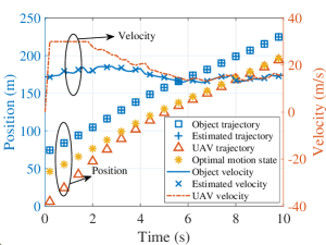
(a) The UAV and object motion state.

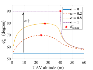
(b) The fixed elevation angle.

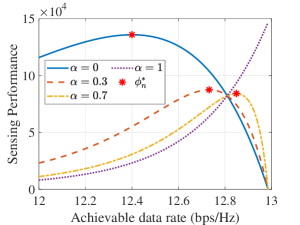
(c) The S&C performance bounds.

Figure 2: Numerical results characterizing the proposed tracking scheme, the fixed elevation angle and the sensing&communication (S&C) performance bounds.

IV Numerical results

In this section, numerical results are provided for characterizing the obtained solution in Section III-A and the optimal relative motion state derived in Section III-B. Unless specified otherwise, the following required parameters are used: $P_{A}=40$ dBm, $N_{sym}=10^{4}$, $\Delta T=0.2$ s, $\lambda=0.01$ m, $f_{c}=30$ GHz, $\sigma^{2}=\sigma_{C}^{2}=-80$ dBm, $\gamma_{C}=11$ bps/Hz, $\tilde{q}=5$, $\varepsilon=100\ \text{m}^{2}$ , $N_{t}=N_{r}=32$, $a_{1}=1$, $a_{2}=1.2\times 10^{-7}$, $a_{3}=600$, and $H=50$ m.

Fig.2(a) shows the trajectories and the velocities of both the UAV and the moving object, together with the estimated object motion state in one trial where the results are picked per $0.6$s and the weighting factor is set as $\alpha=0.5$. Also, the diagonal elements of the state prediction MSE matrix $\mathbf{M}_{p,n}$ and the predicted measurement MSE matrix $\breve{\mathbf{M}}_{m,n}$ at a typical time slot (i.e., $n=40$) are given by $[\mathbf{M}_{p,n}]_{11}=0.014\ \text{m}^{2}$, $[\mathbf{M}_{p,n}]_{22}=1\ \text{m}^{2}\text{s}^{-2}$, $[\breve{\mathbf{M}}_{m,n}]_{11}=2.3\times 10^{-4}\ \text{m}^{2}$ and $[\breve{\mathbf{M}}_{m,n}]_{22}=7.5\times 10^{-6}\ \text{m}^{2}\text{s}^{-2}$, respectively, which represents the case where the predicted measurement MSE dominates the predicted PCRBs. Then, it can be observed from Fig.2(a) that the UAV finally approximates its motion state as the optimal relative motion state $\mathbf{x}_{n}^{*}$, which validates the effectiveness of approximating the obtained solution to (P1) by the optimal solution to (SP1) under the predicted measurement MSE-dominant case. Moreover, the estimated object motion state matches the actual motion state well, which verifies the effectiveness of the proposed tracking scheme.

Fig.2(b) illustrates the varying trends of the fixed elevation angle $\phi_{n}^{*}$ as the UAV altitude $H$ increases under different weighting factors. It can be observed that the fixed elevation angle $\phi_{n}^{*}$ in general first increases but then decreases as the flying altitude $H$ increases. This is expected due to the measurement trade-off: the angle measurement noise variance $\sigma_{1,n}^{2}$ is minimized at $\phi_{n}=\pi/2$, however, the time delay and Doppler shift measurement noise variance $\sigma_{i,n}^{2},i=2,3$ are both minimized at $\phi_{n}=\arctan{\sqrt{2}}$. When the flying altitude $H$ is lower than the altitude that reaches $\phi_{n,max}^{*}$, the role of minimizing $\sigma_{1,n}^{2}$ on the measurement CRB minimization outweighs the counterpart of minimizing $\sigma_{i,n}^{2},i=2,3$, while the reverse holds when the flying altitude $H$ is higher than the altitude that reaches $\phi_{n,max}^{*}$. Furthermore, it is shown that as the priority weight factor $\alpha$ increases from $0$ to $1$, the fixed elevation angle $\phi_{n}^{*}$ generally increases under the same flying height, which illustrates the position-velocity trade-off: the measurement CRB for the relative position is minimized at $\phi_{n}=\pi/2$ when $\xi(H)$ is nonpositive and at $\phi_{n}=\arctan{\sqrt{\chi_{1}}}$ when $\xi(H)$ is positive, however, the counterpart for relative velocity is minimized at $\phi_{n}=\arctan{\sqrt{2}}$.

Fig.2(c) illustrates the varying trends of the sensing performance with the increasing of the communication performance with $a_{1}=0.15$, where the sensing performance is calculated as the inverse of $g(x_{n},0)$ and the communication performance is calculated as the achievable date rate $R_{n}$. As the weighting factor $\alpha$ increases from $0$ to $1$, the sensing-communication performance bound successively approaches the performance bound with $\alpha=1$, which demonstrates the sensing-communication trade-off: the weighted sum of measurement CRBs is minimized at $\phi_{n}=\phi_{n}^{*}$ is satisfied, however, the achievable data rate is maximized at $\phi_{n}=\pi/2$.

V Conclusion

In this work, an EKF-based tracking scheme is proposed for a UAV tracking a moving object, where an efficient solution to the weighted sum-predicted PCRB minimization is obtained based on the SCA method. When the predicted PCRBs are dominated by the predicted measurement MSE, the obtained solution can be approximated by the optimal relative motion state obtained under the measurement MSE-only case, which is proved to sustain a fixed elevation angle and zero relative velocity. Furthermore, simulation results validate the effectiveness of the proposed tracking scheme and the approximation as well as three interesting trade-offs on system performance achieved by the fixed elevation angle. More general scenarios where multiple objects moving along trajectories of arbitrary geometry are worthwhile future works.

References

• [1] F. Liu et al., “Integrated sensing and communications: Toward dual-functional wireless networks for 6G and beyond,” IEEE J. Sel. Areas Commun., vol. 40, no. 6, pp. 1728–1767, Jun. 2022.
• [2] F. Dong et al., “Sensing as a service in 6G perceptive networks: A unified framework for ISAC resource allocation,” IEEE Trans. Wireless Commun., vol. 22, no. 5, pp. 3522–3536, May 2023.
• [3] F. Liu et al., “Radar-assisted predictive beamforming for vehicular links: Communication served by sensing,” IEEE Trans. Wireless Commun., vol. 19, no. 11, pp. 7704–7719, Nov. 2020.
• [4] K. Meng et al., “Throughput maximization for UAV-enabled integrated periodic sensing and communication,” IEEE Trans. Wireless Commun., vol. 22, no. 1, pp. 671–687, Jan. 2023.
• [5] J. Wu, W. Yuan, and L. Hanzo, “When UAVs meet ISAC: Real-time trajectory design for secure communications,” IEEE Trans. Veh. Technol., early access, 2023.
• [6] J. Wu, W. Yuan, and L. Bai, “On the interplay between sensing and communications for UAV trajectory design,” IEEE Internet Things J., vol. 10, no. 23, pp. 20 383–20 395, Dec. 2023.
• [7] P. Kumari, S. A. Vorobyov, and R. W. Heath, “Adaptive virtual waveform design for millimeter-wave joint communication–radar,” IEEE Trans. Signal Process., vol. 68, pp. 715–730, Nov. 2019.
• [8] P. Stoica and A. Nehorai, “MUSIC, maximum likelihood, and Cramer-Rao bound,” IEEE Trans. Acoust., Speech, Signal Process., vol. 37, no. 5, pp. 720–741, May 1989.
• [9] S. M. Kay., Fundamentals of Statistical Signal Processing, Volume 1: Estimation Theory, Englewood Cliffs, NJ, USA: Prentice Hall, 1998.
• [10] Y. Sun, P. Babu, and D. P. Palomar, “Majorization-minimization algorithms in signal processing, communications, and machine learning,” IEEE Trans. Signal Process., vol. 65, no. 3, pp. 794–816, Feb. 2017.
• [11] J. Nocedal and S. J. Wright, Numerical Optimization, Springer, New York, NY, 2004.
• [12] S. Boyd and L. Vandenberghe, Convex Optimization, Cambridge, U.K.:Cambridge Univ. Press, 2004.