Failure of the Mott’s formula for the Thermopower in Carbon Nanotubes
Abstract
The well-known Mott’s formula links the thermoelectric power characterised by Seebeck coefficient to conductivity. We calculate analytically the thermoelectric current and Seebeck coefficient in one-dimensional systems and show that, while the prediction of Mott’s formula is valid for Dirac fermions, it is misleading for the carriers having a parabolic dispersion. We apply the developed formalism to metallic single wall carbon nanotubes and obtain a non-trivial non-monotonic dependence of the Seebeck coefficient on the chemical potential. We emphasize that, in contrast to the Mott’s formula, the classical Kelvin’s formula that links thermoelectric power to the temperature derivative of the chemical potential is perfectly valid in carbon nanotubes in the ballistic regime. Interestingly, however, the Kelvin’s formula fails in two- and three-dimensional systems in the ballistic regime.
pacs:
73.21.-b, 65.40.gdIt is well-known that the low-temperature ballistic conductance in one-dimensional systems is quantized [1]
| (1) |
where is Planck constant while is the number of the quantization subbands situated below the chemical potential [2, 3, 4, 5, 6].
Carbon nanotubes (CNTs) represent an example of a one-dimensional system, where indeed the quantization of conductance has been observed [7]. It is important to note that the conductance takes constant and discrete values independently of the type of electronic dispersion: linear or parabolic. Here we show that in contrast to the conductance the thermoelectric power in carbon nanotubes is strongly dependent on the chemical potential, electronic concentration and temperature. These dependencies are governed by the derivative of the chemical potential over temperature which is proportional to the Seebeck coefficient as it was pointed out by Lord Kelvin in the middle of the XIXth century [8]
| (2) |
The alternative, kinetic approach to the theoretical description of the Seebeck effect was developed by Sir Nevil Mott in the second half of the XXth century [9]. The Mott’s formula relates the Seebeck coefficient to the conductivity of the system:
| (3) |
where is conductivity, is the chemical potential, is temperature. Here and further we assume One can see that substituting the above expression for conductance to the Mott’s formula one obtains for any value of chemical potential except the close vicinity of the bottoms of the quantisation subband. Below we demonstrate that this simple conclusion fails and the Mott’s formula is unable to describe the thermoelectric phenomena in 1D systems in the ballistic regime. In contrast, the Kelvin’s formula remains valid in the ballistic regime in any one-dimensional (1D) system. Interestingly, however, the Kelvin’s formula turns out to be no more valid in two- and three-dimensional (2D and 3D) systems, in the ballistic regime.
The thermocurrent and thermoelectricity in the ballistic regime have been carefully studied theoretically in 1D, 2D and 3D systems [10, 11, 12]. The difference between these works and our present work is that we focus on the broken circuit geometry where no electric current is flowing through the system. We present an analytical theory of the Seebeck effect in metallic CNTs in the regime of a ballistic transport. We note that the Seebeck coefficient is also a direct measure of the entropy per particle, which makes it one of the most important characteristics of the statistics of quasiparticles in crystals [13]. We find that, in CNTs, it is dramatically dependent on the type of electronic dispersion. In the case of a parabolic dispersion, the Seebeck coefficient is a non-monotonic function of the chemical potential. Its magnitude decreases with the increase of the chemical potential, and its sign changes in the vicinity of the resonances of the chemical potentials and bottom energies of the electron and hole quantization subbands. In contrast,in the case of a linear dispersion that is observed in the vicinity of Dirac points in conducting CNTs the Seebeck coefficient is equal to zero. The sharp contrast between the behaviors of conductivity and Seebeck coefficient as functions of the chemical potential that may be efficiently controlled by an applied bias opens room for a variety of non-trivial effects governed by an interplay of currents induced by electric field and temperature gradient.
Recovering of the Kelvin’s formula for Seebeck coefficient in the ballistic regime for a 1D system. The definition of the Seebeck coefficient in the case of a broken electric circuit (, where is an electric current) reads
| (4) |
Here is the difference of temperatures at the edges of a channel and is the voltage induced due to the Seebeck effect. We note that the induction of the voltage results in the appearance of a ballistic current
| (5) |
with being the Fermi-Dirac distribution, being the electron energy. In its turn, the temperature difference applied at the edges of the channel also will generate the current
| (6) |
The density of states of electrons entering a 1D channel can be written as follows
| (7) |
Here and in what follows we assume the degeneration factor of quantum states . The results can be easily generalized for any other value of . The electronic velocity is defined by the general relation:
| (8) |
No surprises, their product turns out to be constant
The condition of a broken circuit imposes that the total current in the channel is zero. This condition implies the compensation of the currents (5) and (6). Expansion of the Fermi-Dirac functions in the limit results in the equality
| (9) |
The second term is an odd function of energy, hence after integration it yields zero. In what concerns the partial derivatives of the Fermi-Dirac distribution function over energy and chemical potential, their absolute values are equal while their signs are opposite:
The remaining integration in Eq. (9) is trivial and it leads to
| (10) |
This, in view of the definition (4) yields the Kelvin’s formula (2). We conclude that the Kelvin’s formula is perfectly valid in any 1D system in the ballistic regime.
Here we would like to point out that in 2D and 3D cases the similar reasoning is also possible, however, the product of the density of states and the electronic velocity appears to be energy dependent. Hence, it cannot be simplified as it was done above. This is why, the equivalent of the second term in Eq. (9) would not be equal to zero. An important implication of this is the failure of the Kelvin’s formula in 2D and 3D cases in the ballistic regime.
Coming back to the 1D case, one can rewrite the Kelvin’s formula in terms of the logarithmic derivative of DOS (see Supplemental Material, Sec. S1 [14]).
| (11) |
Conductance and the Mott’s formula for 1D two-subband system in ballistic regime. It is instructive to compare the exact expression for the Seebeck coefficient obtained above with an approximation that follows from the Mott’s formula. In order to derive it, we start from the generic expression for the electric current density in a one-dimensional channel in the ballistic regime (5).
We assume that the applied voltage is small, so that . For simplicity, in DOS we shall only account for the contributions of two energy subbands of the CNT. We shall assume that the chemical potential is close to the bottom of the second subband from the either positive or negative side. In this case, DOS may be written as
| (12) |
where is the bottom of the second subband. Now one can find the conductance as
| (13) |
This expression can be now substituted to the Mott’s formula (3). As a result we obtain:
| (14) |
One can see that in the limit of the Seebeck coefficient calculated in this way appears to be exponentially small. Below we will show that this prediction of the Mott’s formula strongly deviates from one of the Kelvin’s formula confirmed by the exact microscopic consideration (Eqs. (5)-(10)).
The specific case of a metallic CNT. Energy spectra of single-walled carbon nanotubes.
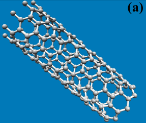
Basic electronic properties of single-walled (dubbed originally as single-shell [15]) carbon nanotubes (CNTs) have been well-understood for over three decades [16] and depend entirely on their chirality , where (as explained in detail in Ref. [17]) the numbers express the wrapping ‘chiral’ vector connecting two carbon sites along the nanotube circumference via the two unit vectors of the underlying hexagonal graphene lattice. A CNT with , where is an integer, is a quasi-one-dimensional semiconductor with the band gap inversely proportional to the nanotube radius pm, where the graphene lattice constant with Å being a distance between neighbouring carbon atoms in graphene. Only armchair nanotubes are truly metallic (gapless) with the low-energy part of dispersion well-described by , where m/s is the Fermi velocity in graphene and .
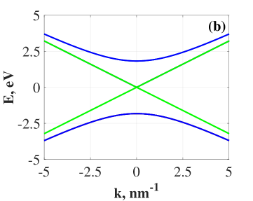
The low-lying branches of CNT spectra, which are relevant for this work, are well described by cross-sections of the famous graphene cone for the quantized values of the wave number along the CNT rolling direction (chiral vector). Thus, in the vicinity of the Dirac point the energy spectrum of an electron in the -th subband is given by
| (15) |
For the two branches closest to the Dirac point (), for the metallic and quasi-metallic CNTs . The bottoms of their higher subbands are given by . Notably, the subbands with are reasonably-well described by the effective mass approximation with .
The specific case of a metallic CNT. A vanishing contribution to the Seebeck coefficient from linear dispersion subbands. For the linear dispersion subband DOS is constant and given by , where is the sound velocity. As a result, the temperature derivative of the concentration of charge carriers turns zero. Hence the Dirac mode does not contribute to the Seebeck coefficient in agreement with both the Kelvin’s and Mott’s formulae. This statement remains valid also in the vicinity of the Dirac point due to the compensation of electron and hole contributions to the Seebeck effect (see Supplemental Material, Sec. S2 [14]).
Conflicting predictions of the Kelvin’s and Mott’s approaches for the contributions of parabolic subbands to the Seebeck coefficient.
DOS in parabolic subbands can be found as:
| (16) |
where is the maximum possible value of such as still remains positive.
Using the expressions for DOS and its derivative one easily finds:
| (17) |
The dependence of the Seebeck coefficient on the chemical potential calculated at different temperatures is shown in Fig. 3. One can notice the strong difference in the results obtained following the Kelvin’s approach (red lines) and Mott’s approach (blue lines). The Kelvin’s approach predicts the hyperbolic decay of the Seebeck coefficient away from the resonance between the chemical potential and the bottom of the subband. At the resonance point, the singularity and the change of sign of the Seebeck coefficient are observed. In contrast, the Mott’s formula predicts a finite value of the Seebeck coefficient at the bottom of subband, no sign change and a fast exponential decay away from the resonance. We note at this point that long ago the change of the sign of the Seebeck coefficient was identified as a signature of the topological phase transition which indeed takes place ones the chemical potential crosses the bottom of the next quantization subband [18, 19, 20, 21, 22, 23, 24]. The divergence of Seebeck coefficient in absence of scattering is caused by the singularity in DOS. It disappears once the smearing of the density of states is taken into account as we show in the next section.
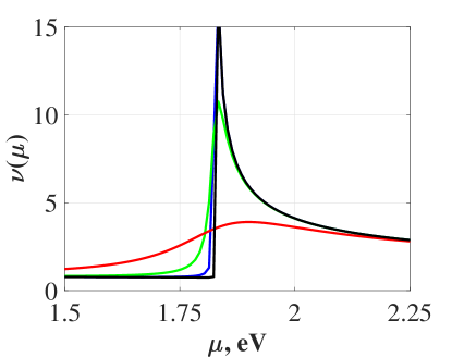
Effect of smearing of DOS in parabolic subbands. The Kelvin’s formula. In any realistic 1D system including CNTs, singularities of DOS are smeared due to a variety of factors: from finite size effects to fluctuations and non-linearities. Therefore, it is important to consider an effect of smearing of DOS on the Seebeck coefficient in the ballistic regime. The Green function of an electron in a single-wall CNT is
| (18) |
where is the positive parameter responsible for the smearing effect and is the continuous momentum along the -direction.
For the calculation of DOS one can use the standard expression [25]:
| (19) |
Performing the momentum integration and making the correct choice of the branch of the logarithm one finds
| (20) |
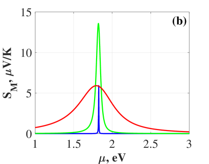
where the square root is taken in the arithmetic sense (positive value). The calculated smeared DOS is presented in Fig. 2 .
Now one can derive the exact expression for the contribution to the Seebeck coefficient of a CNT coming from parabolic energy subbands:
| (21) |
The dependence of the Seebeck coefficient on the chemical potential calculated at different values of smearing is presented in Fig. 3.
Effect of smearing of DOS in parabolic subbands. The Mott’s formula. The smearing of the density of states jump in Eq. (12) will also affect the Mott’s formula for the Seebeck coefficient. Below we consider a relatively clean system and the range of not too low temperatures: Within the Lorentz approximation for delta function and using the relation , one can present -function in Eq. (12) in the form
| (22) |
This allows to account in Eq. (14) for the smearing of DOS. At the same time, temperatures are supposed to be low enough to exclude mixing of electrons belonging to different subbands.
The conductance is no more given by Eq. (13). Instead, it acquires the form
| (23) |
Integration of the second term by parts followed by the application of the Cauchy’s theorem (see Supplemental Material, Sec. S3 [14]) yields the conductivity explicitly:
| (24) |
Substituting it to the Mott’s formula one obtains the Seebeck coefficient:
| (25) |
Here is the digamma-function (logarithmic derivative of the Euler gamma-function) [1].
In the limiting cases when the chemical potential is either close to the bottom of the parabolic subband or sufficiently far from it one finds
One can verify that in the limit of this expression reproduces Eq. (14) [27].
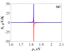
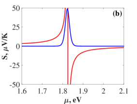
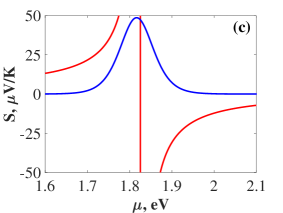
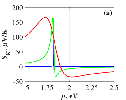
Figure 4 (a,b) shows the results of calculation of the Seebeck coefficient as a function of the chemical potential in the vicinity of the bottom of the second subband performed accounting for the smearing of DOS. The curves in the panels (a) and (b) are calculated with use of the Kelvin’s and Mott’s approaches, respectively. One can see that even in the case of a strong smearing Kelvin’s and Mott’s approaches yield qualitatively different results, especially in what concerns the change of sign of the Seebeck coefficient in the vicinity of the topological phase transition point.
In conclusion, the ballistic regime offers peculiar modifications of some well-known thermoelectric relations. In particular, it turns out that the Mott’s formula for the Seebeck effect is incorrect for one-dimensinal parabolic bands, while the Kelvin’s formula remains fully accurate in this case. The differences between two approaches become apparent in the vicinity of resonances between the electronic chemical potential and the bottoms of energy subbands characterised by parabolic dispersions. The Mott’s formula predicts a finite value of the Seebeck coefficient at the resonance and no change of sign. In contrast, the Kelvin’s formula predicts divergence and the change of sign of the Seebeck coefficient at the resonance between the chemical potential and the bottom of a parabolic subband. The latter result is characteristic of most of topological phase transitions that occur once a new energy subband comes into play. Our analysis shows that both Kelvin’s and Mott’s expressions predict zero contributions to the Seebeck coefficient from the linear dispersion band in metallic CNTs in the ballistic regime. In contrast, the contribution of parabolic bands is not zero even far from the resonance points, according to the Kelvin’s (but not Mott’s!) formula. This conclusion can be easily verified experimentally. Any deviation of the Seebeck coefficient of CNTs from zero in the ballistic regime would characterize the inaccuracy of the Mott’s formula. Finally, we note that in 2D and 3D cases, the Kelvin’s formula also fails in the ballistic regime. This is because counter-propagating non-dissipative currents of ”hot” and ”cold” electrons are formed due to the combined actions of the temperature and voltage drops in these cases. The total electric current remains zero, but the system cannot be described by a single electro-chemical potential. We are looking forward for the experimental manifestations of these theoretical results.
References
- [1] C. W. J. Beenakker and H. van Houten, in Solid State Physics, 44, (H. Ehrenreich and D. Turnbull, eds., Academic Press, Boston), pp. 1-228 (1991).
- [2] D. A. Wharam, T. J. Thornton, R. Newbury, M. Pepper, H. Ahmed, J. E. F. Frost, D. G. Hasko, D. C. Peacock, D. A. Ritchie and G. A. C. Jones. J. Phys. C 21, L209 (1988).
- [3] B. J. van Wees, H. van Houten, C. W. J. Beenakker, J. G. Williamson, L. P. Kouwenhoven, D. van der Marel, and C. T. Foxon Phys. Rev. Lett. 60, 848 (1988).
- [4] K. von Klitzing and G. Dorda, and M. Pepper, Phys. Rev. Lett. 45, 494 (1980).
- [5] D. C. Tsui, H. L. Stormer, A. C. Gossard, Phys. Rev. Lett. 48, 1559 (1982).
- [6] T. Ando, A. B. Fowler and F. Stern, Rev. Mod. Phys. 54 437 (1982).
- [7] M. P. Anantram and F. Lèonard, Rep. Prog. Phys. 69, 507 (2006).
- [8] W. Thomson (Lord Kelvin), Collected Papers I, Proc. R. Soc. Edinburgh 123, 237 (1854).
- [9] P. M. Chaikin and G. Beni, Phys. Rev. B 13, 647 (1976); R. R. Heikes, Thermoelectricity (Wiley-Interscience, New York, 1961).
- [10] U. Sivan and Y. Imry, Phys. Rev. B 33, 551 (1986).
- [11] V. L. Gurevich and A. Thellung, Phys. Rev. B 65, 153313 (2002).
- [12] C. R. Proetto, and C. E.T. Goncales da Silva, Solid State Comm., 80, 909 (1991).
- [13] M. R. Peterson, and B. S. Shastry, Phys. Rev. B 82, 195105 (2010).
- [14] See Supplemental Material for details.
- [15] S. Iijima and T. Ichihashi, Nature 363, 603 (1993)
- [16] R. Saito, M. Fujita, G. Dresselhaus, and M. S. Dresselhaus, Phys. Rev. B 46, 1804 (1992).
- [17] R. Saito, G. Dresselhaus, and M. S. Dresselhaus, Physical Properties of Carbon Nanotubes (Imperial College Press, London, 1998).
- [18] V. S. Egorov and A. N. Fedorov, JETP Lett. 35, 462 (1982).
- [19] A. A. Varlamov and A. V. Pantsulaya, Sov. Phys. JETP 62, 1263 (1985).
- [20] A. N. Velikodnyi, N. V. Zavaritskii, T. A. Ignateva, and A. A. Yurgens, JETP Lett. 43, 773 (1986).
- [21] A. A. Varlamov, V. Egorov, and A. Pantsulaya, Adv. Phys. 38, 469 (1989).
- [22] Y. M. Blanter, M. I. Kaganov, A. V. Pantsulaya, and A. A. Varlamov, Phys. Rep. 245, 159 (1994).
- [23] A. Pourret et al, J. Phys. Soc. Jpn. 88, 104702 (2019).
- [24] H. Pfau, et al, Phys. Rev. Lett. 119, 126402 (2017).
- [25] A. A. Abrikosov, L. P. Gor’kov, I. E. Dzyaloshinski, The Methods of Quantum Field Theory in Statistical Physics, Dover Publications, New York (1963).
- [26] M. Abramowitz and I.A. Stegun, (Eds.). Handbook of Mathematical Functions with Formulas, Graphs, and Mathematical Tables, 9th printing. New York: Dover, 1972.
- [27] We note here that dealing with the Taylor expansion of the polygamma-functions we were not able to reproduce exponentially small asymptotics of Eq. (14) far from the bottom of the parabolic band (when ), but simply obtained zero.
Supplemental material for “Failure of the Mott’s formula for the Thermopower in Carbon Nanotubes”
I S1: The link between the temperature derivative of the chemical potential and the density of states
Indeed, the temperature derivative of the chemical potential can be expressed as follows:
| (S1) |
The relationship between the electronic concentration , the chemical potential and the temperature can be found by integrating the density of electron states multiplied by the Fermi-Dirac distribution over energy:
| (S2) |
Required derivatives can be easily obtained in the general form
| (S3) |
and
| (S4) |
Hence
| (S5) |
II S2: The vicinity of the Dirac point
In the vicinity of the Dirac point, both electron and hole concentrations are different from zero at non-zero temperature. Below we will take into account the dependence of chemical potential on temperature in order to evaluate both electron and hole contributions to the Seebeck coefficient.
| (S6) |
where we introduced the chemical potential for holes . Due to the possible nonzero charge of the system,
| (S7) |
Here is the overall charge density. Substituting Eq. (S6) in Eq. (S7) and performing integration one finds
| (S8) |
Thus, one can see that the chemical potential for the linear dispersion branch depends on the total charge density only and it does not depend on temperature. This means that and corresponding Seebeck coefficient is zero for the whole linear branch including the vicinity of the Dirac point:
| (S9) |
II.1 The special point
Here we address the special case of the chemical potential resonant with the Dirac point. We already saw that and . Let us substitute these relations to the above derivatives to the general thermodynamic expression relating the entropy per particle with partial temperature derivative of the chemical potential
| (S10) |
One can see that at the point the number of electrons coincides with the number of holes (), i.e. the first multiplier in Eq. (S10) turns zero, while with use of Eq. (S6) it is easy to find that the second multiplier is equal to . Hence, the entropy per particle and Seebeck coefficient in the Dirac point turn out to be equal to zero:
III S3: Derivation of the expression for conductivity
Here we provide the detailed calculation of the integral for conductivity:
| (S11) |
We split integral Eq. (S11) into parts , where
| (S12) |
and
| (S13) |
Applying integration by parts to Eq. (S13) one can rewrite the integral as
| (S14) |
The latter integral can be evaluated using the Cauchy’s theorem by means of residues. The appearing summation over the poles of can be performed in terms of digamma-function and after straightforward calculations one finds:
| (S15) |
where the symmetry property of the digamma function was applied [1].
Therefore, the final result for conductivity is expressed as
| (S16) |
References
- [1] M. Abramowitz and I.A. Stegun, (Eds.). Handbook of Mathematical Functions with Formulas, Graphs, and Mathematical Tables, 9th printing. New York: Dover, 1972.