Project and Conquer: Fast Quantifier Elimination for Checking Petri Net Reachability

Abstract

We propose a method for checking generalized reachability properties in Petri nets that takes advantage of structural reductions and that can be used, transparently, as a pre-processing step of existing model-checkers. Our approach is based on a new procedure that can project a property, about an initial Petri net, into an equivalent formula that only refers to the reduced version of this net. Our projection is defined as a variable elimination procedure for linear integer arithmetic tailored to the specific kind of constraints we handle. It has linear complexity, is guaranteed to return a sound property, and makes use of a simple condition to detect when the result is exact. Experimental results show that our approach works well in practice and that it can be useful even when there is only a limited amount of reductions. Keywords— Petri nets; Quantifier elimination; Reachability problems.

1 Introduction

We describe a method to accelerate the verification of reachability properties in Petri nets by taking advantage of structural reductions [Ber87]. We focus on the verification of generalized properties, that can be expressed using a Boolean combination of linear constraints between places, such as $(2\,p_{0}+p_{1}=5)\land(p_{1}\geqslant p_{2})$ for example. This class of formulas corresponds to the reachability queries used in the Model Checking Contest (MCC) [ABC⁺19], a competition of Petri net verification tools that we use as a benchmark.

In essence, net reductions are a class of transformations that can simplify an initial net, $(N_{1},m_{1})$, into another, residual net $(N_{2},m_{2})$, while preserving a given class of properties. This technique has become a conventional optimization integrated into several model-checking tools [BLBDZ18, BDJ⁺19, TM21]. A contribution of our paper is a procedure to transform a property $F_{1}$, about the net $N_{1}$, into a property $F_{2}$ about the reduced net $N_{2}$, while preserving the verdict. We have implemented this procedure into a new tool, called Octant [Ama23], that can act as a pre-processor allowing any model-checker to transparently benefit from our optimization. Something that was not possible in our previous works. In practice, it means that we can use our approach as a front-end to accelerate any model-checking tool that supports generalized reachability properties, without modifying them.

Our approach relies on a notion, called polyhedral reduction [ABD21, ABD22, ADZLB21, BLBDZ19], that describes a linear dependence relation, $E$, between the reachable markings of a net and those of its reduced version. This equivalence, denoted $(N_{1},m_{1})\mathop{\equiv_{E}\,}(N_{2},m_{2})$, preserves enough information in $E$ so that we can rebuild the state space of $N_{1}$ knowing only the one of $N_{2}$. An interesting application of this relation is the following reachability conservation theorem [ABD21]: assume we have $(N_{1},m_{1})\mathop{\equiv_{E}\,}(N_{2},m_{2})$, then property $F$ is reachable in $N_{1}$ if and only if $E\land F$ is reachable in $N_{2}$. This property is interesting since it means that we can apply more aggressive reduction techniques than, say, slicing [Rak12, LOST17, KKG18], cone of influence [CJGK⁺18], or other methods [GRVB08, KBJ21] that seek to remove or gather together places that are not relevant to the property we want to check. We do not share this restriction in our approach, since we reduce nets beforehand and can therefore reduce places that occur in the initial property. We could argue that approaches similar to slicing only simplify a model with respect to a formula, whereas, with our method, we simplify the model as much as possible and then simplify formulas as needed. This is more efficient when we need to check several properties on the same model and, in any case, nothing prevents us from applying slicing techniques on the result of our projection.

However, there is a complication, arising from the fact that the formula $E\land F$ may include variables (places) that no longer occur in the reduced net $N_{2}$, and therefore act as existentially quantified variables. This can complicate some symbolic verification techniques, such as $k$-induction [SSS00], and impede the use of explicit, enumerative approaches. Indeed, in the latter case, it means that we need to solve an integer linear problem for each new state, instead of just evaluating a closed formula. To overcome this problem, we propose a new method for projecting the formula $E\land F$ into an equivalent one, $F^{\prime}$, that only refers to the places of $N_{2}$. We define our projection as a procedure for quantifier elimination in Presburger Arithmetic (PA) that is tailored to the specific kind of constraints we handle in $E$. Whereas quantifier elimination has an exponential complexity in general for existential formulas, our construction has linear complexity and can only decrease the size of a formula. It also always terminates and returns a result that is guaranteed to be sound; meaning it under-approximates the set of reachable models and, therefore, a witness of $F^{\prime}$ in $N_{2}$ necessarily corresponds to a witness of $F$ in $N_{1}$. Additionally, our approach includes a simple condition on $F$ that is enough to detect when our result is exact, meaning that if $F^{\prime}$ is unreachable in $N_{2}$, then $F$ is unreachable in $N_{1}$. We show in Sect. 6 that our projection is complete for $80\%$ of the formulas used in the MCC.

Outline and Contributions.

We start by giving some technical background about Petri nets and the notion of polyhedral abstraction in Sect. 2, then describe how to use this equivalence to accelerate the verification of reachability properties (Th. 3.1 in Sect. 3). We also use this section to motivate our need to find methods to eliminate (or project) variables in a linear integer system. We define our fast projection method in Sect. 4, which is based on a dedicated graph structure, called Token Flow Graph (TFG), capturing the particular form of constraints occurring with polyhedral reductions. We prove the correctness of this method in Sect. 5. Our method has been implemented, and we report on the results of our experiments in Sect. 6. We give quantitative evidence about several natural questions raised by our approach. We start by proving the effectiveness of our optimization on both $k$-induction and random walk. Then, we show that our method can be transparently added as a preprocessing step to off-the-shelf verification tools. This is achieved by testing our approach with the three best-performing tools that participated in the reachability category of the MCC—ITS-Tools [TM15] (or ITS for short); LoLA [Wol18]; and TAPAAL [DJJ⁺12]—which are already optimized for the type of models and formulas used in our benchmark. Our results show that reductions are effective on a large set of queries and that their benefits do not overlap with other existing optimizations, an observation that was already made in [ABD22, BDJ⁺19]. We also prove that our procedure often computes an exact projection and compares favorably well with the variable elimination methods implemented in isl [Ver10] and Redlog [DS97]. This supports our claim that we are able to solve non-trivial quantifier elimination problems.

2 Petri Nets and Polyhedral Abstraction

Most of our results involve non-negative integer solutions to constraints expressed in Presburger Arithmetic, the first-order theory of the integers with addition [Haa18]. We focus on the quantifier-free fragment of PA, meaning Boolean combinations (using $\land$, $\lor$ and $\neg$) of atomic propositions of the form $\alpha\sim\beta$, where $\sim$ is one of $=,\leqslant$ or $\geqslant$, and $\alpha,\beta$ are linear expressions with coefficients in $\mathbb{Z}$. Without loss of generality, we can consider only formulas in disjunctive normal form (DNF), with linear predicates of the form $(\sum k_{i}\,x_{i})+b\geqslant 0$. We deliberately do not add a divisibility operator $k\mid\alpha$, which requires that $k$ evenly divides $\alpha$, since it can already be expressed with linear predicates, though at the cost of an extra existentially quantified variable. This fragment corresponds to the set of reachability formulas supported by many model-checkers for Petri nets, such as [ABB⁺16, BRV04, DJJ⁺12, TM15, Wol18].

We use $\mathbb{N}^{V}$ to denote the space of mappings over $V=\{x_{1},\dots,x_{n}\}$, meaning total mappings from $V$ to $\mathbb{N}$. We say that a mapping $m$ in $\mathbb{N}^{V}$ is a model of a quantifier-free formula $F$ if the variables of $F$, denoted $\mathsf{fv}({F})$, are included in $V$ and the closed formula $F\{m\}$ (the substitution of $m$ in $F$) is true. We denote this relation $m\models F$.

$$F\{m\}\ \triangleq\ F\{x_{1}\leftarrow m(x_{1})\}\dots\{x_{n}\leftarrow m(x_{n})\}$$ (1)

We say that a Presburger formula is consistent when it has at least one model. We can use this notion to extend the definition of models in the case where $F$ is over-specified; i.e. it has a larger support than $m$. If $m^{\prime}\in\mathbb{N}^{U}$ with $U\subseteq\mathsf{fv}({F})$, we write $m^{\prime}\models F$ when $F\{m^{\prime}\}$ is consistent.

Petri Nets and Reachability Formulas.

A Petri net $N$ is a tuple $(P,T,\mathrm{Pre},\allowbreak\mathrm{Post})$ where $P=\{p_{1},\dots,p_{n}\}$ is an ordered set of places, $T=\{t_{1},\dots,t_{k}\}$ is a finite set of transitions (disjoint from $P$), and $\mathrm{Pre}:T\rightarrow\mathbb{N}^{P}$ and $\mathrm{Post}:T\rightarrow\mathbb{N}^{P}$ are the pre- and post-condition functions (also called the flow functions of $N$). A state $m$ of a net, also called a marking, is a mapping of $\mathbb{N}^{P}$. A marked net $(N,m_{0})$ is a pair composed of a net and its initial marking $m_{0}$.

We extend the comparison $(=,\geqslant)$ and arithmetic operations $(-,+)$ to their point-wise equivalent. With our notations, a transition $t\in T$ is said enabled at marking $m$ when $m\geqslant\mathrm{Pre}(t)$. A marking $m^{\prime}$ is reachable from a marking $m$ by firing transition $t$, denoted $m\mathbin{\smash[t]{\mathrel{\mathop{\mathord{\smash{-}}\mkern-6.0mu\cleaders\hbox{$\mkern-2.0mu\mathord{\smash{-}}\mkern-2.0mu$}\hfill\mkern-6.0mu\mathord{\rightarrow}}\limits^{\ t\ }}}}m^{\prime}$, if: (1) transition $t$ is enabled at $m$; and (2) $m^{\prime}=m-\mathrm{Pre}(t)+\mathrm{Post}(t)$. When the identity of the transition is unimportant, we simply write this relation $m\mathbin{\smash[t]{\mathrel{\mathop{\mathord{\smash{-}}\mkern-6.0mu\cleaders\hbox{$\mkern-2.0mu\mathord{\smash{-}}\mkern-2.0mu$}\hfill\mkern-6.0mu\mathord{\rightarrow}}\limits^{\ \ }}}}m^{\prime}$. More generally, a marking $m^{\prime}$ is reachable from $m$ in $N$, denoted $m\mathbin{\smash[t]{\mathrel{\mathop{\mathord{\smash{-}}\mkern-6.0mu\cleaders\hbox{$\mkern-2.0mu\mathord{\smash{-}}\mkern-2.0mu$}\hfill\mkern-6.0mu\mathord{\rightarrow}}\limits^{\ \ }}}}^{\star}m^{\prime}$ if there is a (possibly empty) sequence of transitions such that $m\mathbin{\smash[t]{\mathrel{\mathop{\mathord{\smash{-}}\mkern-6.0mu\cleaders\hbox{$\mkern-2.0mu\mathord{\smash{-}}\mkern-2.0mu$}\hfill\mkern-6.0mu\mathord{\rightarrow}}\limits^{\ \ }}}}\dots\mathbin{\smash[t]{\mathrel{\mathop{\mathord{\smash{-}}\mkern-6.0mu\cleaders\hbox{$\mkern-2.0mu\mathord{\smash{-}}\mkern-2.0mu$}\hfill\mkern-6.0mu\mathord{\rightarrow}}\limits^{\ \ }}}}m^{\prime}$. We denote $R(N,m_{0})$ the set of markings reachable from $m_{0}$ in $N$.

We are interested in the verification of properties over the reachable markings of a marked net $(N,m_{0})$, with a set of places $P$. Given a formula $F$ with variables in $P$, we say that $F$ is reachable if there exists at least one reachable marking, $m\in R(N,m_{0})$, such that $m\models F$. We call such marking a witness of $F$. Likewise, $F$ is said to be an invariant when all the reachable markings of $(N,m_{0})$ are models of $F$. This corresponds to the two classes of queries found in our benchmark: $\mathrm{EF}\,F$, which is true only if $F$ is reachable; and $\mathrm{AG}\,F$, which is true when $F$ is an invariant, with the classic relationship that $\mathrm{AG}\,F\equiv\neg\,(\mathrm{EF}\,\neg F)$. Examples of properties we can express in this way include: checking if some transition can possibly be enabled, checking if there is a deadlock, checking whether some linear invariant between places is always true, etc.

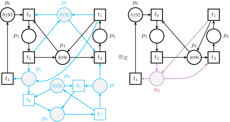
Figure 1: An example of Petri net, $M_{1}$ (left), and one of its polyhedral abstractions, $M_{2}$ (right), with $E\triangleq(p_{1}=p_{4}+4096)\wedge(p_{6}=p_{0}+p_{2}+p_{3}+p_{5}+p_{7})\wedge(a_{1}=p_{7}+p_{8})\wedge(a_{2}=a_{1}+p_{5})$. Colors are used to emphasize places that are either removed or added.

We use a standard graphical notation for nets where places are depicted with circles and transitions with squares. We give an example in Fig. 1, where net $M_{1}$ depicts the SmallOperatingSystem model, borrowed from the MCC benchmark [Kor15]. This net abstracts the lifecycle of a task in a simplified operating system handling several memory segments (place $p_{0}$), disk controller units ($p_{4}$), and cores ($p_{6}$). The initial marking of the net gives the number of resources available (e.g., there are $8\,192$ available memory segments in our example).

We chose this model since it is one of the few examples in our benchmark that fits on one page. This is not to say that the example is simple. Net $M_{1}$ has about $10^{17}$ reachable states, which means that it is out of reach of enumerative methods, and only one symbolic tool in the MCC is able to generate its whole state space [KBG⁺22]. For comparison, the reduced net $M_{2}$ has about $10^{10}$ states.

Polyhedral Abstraction.

We recently defined an equivalence relation that describes linear dependencies between the markings of two different nets, $N_{1}$ and $N_{2}$ [ABD22]. In the following, we reserve $F$ for formulas about a single net and use $E$ to refer to relations. Assume $m$ is a mapping of $\mathbb{N}^{V}$. We can associate $m$ to the linear predicate $\underline{m}$, which is a formula with a unique model $m$.

$$\underline{m}\ \triangleq\ \bigwedge\{x=m(x)\mid x\in V\}$$ (2)

By extension, we say that $m$ is a (partial) solution of $E$ if the system $E\wedge\underline{m}$ is consistent. In some sense, we use $\underline{m}$ as a substitution, since the formulas $E\{m\}$ and $E\land\underline{m}$ have the same models. Given two mappings $m_{1}\in\mathbb{N}^{V_{1}}$ and $m_{2}\in\mathbb{N}^{V_{2}}$, we say that $m_{1}$ and $m_{2}$ are compatible when they have equal values on their shared domain: $m_{1}(x)=m_{2}(x)$ for all $x$ in $V_{1}\cap V_{2}$. This is a necessary and sufficient condition for the system $\underline{m_{1}}\wedge\underline{m_{2}}$ to be consistent. Finally, we say that $m_{1}$ and $m_{2}$ are related up-to $E$, denoted $m_{1}\mathop{\equiv_{E}\,}m_{2}$, when $E\wedge\underline{m_{1}}\wedge\underline{m_{2}}$ is consistent.

$$m_{1}\mathop{\equiv_{E}\,}m_{2}\quad\Leftrightarrow\quad\exists m\in\mathbb{N}^{V}\;.\;m\models E\wedge\underline{m_{1}}\wedge\underline{m_{2}}$$ (3)

This relation defines an equivalence between markings of two different nets ($\mathop{\equiv_{E}\,}\subseteq\mathbb{N}^{P_{1}}\times\mathbb{N}^{P_{2}}$) and, by extension, can be used to define an equivalence between nets themselves, that we call polyhedral equivalence.

Definition 2.1 ($E$-equivalence).

We say that $(N_{1},m_{1})$ is $E$-equivalent to$(N_{2},m_{2})$, denoted $(N_{1},m_{1})\equiv_{E}(N_{2},m_{2})$, if and only if:

(A1)

$E\wedge\underline{m}$ is consistent for all markings $m$ in $R(N_{1},m_{1})$ or $R(N_{2},m_{2})$;

(A2)

initial markings are compatible: $m_{1}\mathop{\equiv_{E}\,}m_{2}$;

(A3)

assume $m^{\prime}_{1},m^{\prime}_{2}$ are markings of $N_{1},N_{2}$, such that $m^{\prime}_{1}\mathop{\equiv_{E}\,}m^{\prime}_{2}$, then $m_{1}^{\prime}$ is reachable iff $m_{2}^{\prime}$ is reachable: $m^{\prime}_{1}\in R(N_{1},m_{1})\iff m_{2}^{\prime}\in R(N_{2},m_{2})$.

By definition, given the equivalence $(N_{1},m_{1})\equiv_{E}(N_{2},m_{2})$, every marking $m^{\prime}_{2}$ reachable in $N_{2}$ can be associated to a subset of markings in $N_{1}$, defined from the solutions to $E\wedge\underline{m^{\prime}_{2}}$ (by condition (A1) and (A3)). In practice, this gives a partition of the reachable markings of $(N_{1},m_{1})$ into “convex sets”—hence the name polyhedral abstraction—each associated with a reachable marking in $N_{2}$. This approach is particularly useful when the state space of $N_{2}$ is very small compared to the one of $N_{1}$.

We can prove that the two marked nets in our running example satisfy $M_{1}\mathop{\equiv_{E}\,}M_{2}$, for the relation $E$ defined in Fig. 1. Net $M_{2}$ is obtained automatically from $M_{1}$ by applying a set of reduction rules, iteratively, and in a compositional way. This process relies on the reduction system defined in [BLBDZ19, ABD22]. As a result, we manage to remove five places: $p_{1},p_{5},p_{6},p_{7},p_{8}$, and only add a new one, $a_{2}$. The “reduction system” ($E$) also contains an extra variable, $a_{1}$, that does not occur in any of the nets. It corresponds to a place that was introduced and then removed in different reduction steps.

Polyhedral abstractions are not necessarily derived from reductions, but reductions provide a way to automatically find interesting instances of abstractions. Also, the equation systems obtained using structural reductions exhibit a specific structure, that we exploit in Sect. 4.

3 Combining Polyhedral Abstraction with Reachability

We can define a counterpart to our notion of polyhedral abstraction which relates to reachability formulas. We show that this equivalence can be used to speed up the verification of properties by checking formulas on a reduced net instead of the initial one (see Th. 3.1 and its corollary, below). In the following, we assume that we have two marked nets such that $(N_{1},m_{1})\equiv_{E}(N_{2},m_{2})$. Our goal is to define a relation $F_{1}\mathop{\equiv_{E}\,}F_{2}$, between reachability formulas, such that $F_{1}$ and $F_{2}$ have the same truth values on equivalent models, with respect to $E$.

Definition 3.1 (Equivalence between formulas).

Assume $F_{1},F_{2}$ are reachable formulas with respective sets of variables, $V_{1}$ and $V_{2}$, in the support of $E$. We say that formula $F_{2}$ implies $F_{1}$ up-to $E$, denoted $F_{2}\mathop{\sqsubseteq_{E}}F_{1}$, if for every marking $m_{2}^{\prime}\in\mathbb{N}^{V_{2}}$ such that $m^{\prime}_{2}\models E\land F_{2}$ there exists at least one marking $m_{1}^{\prime}\in\mathbb{N}^{V_{1}}$ such that $m_{1}^{\prime}\mathop{\equiv_{E}\,}m_{2}^{\prime}$ and $m^{\prime}_{1}\models E\land F_{1}$.

$$F_{2}\mathop{\sqsubseteq_{E}}F_{1}\quad\text{iff}\quad\forall m^{\prime}_{2}.\left(m^{\prime}_{2}\models E\land F_{2}\right)\,\Rightarrow\,\exists m^{\prime}_{1}.\left(m^{\prime}_{1}\mathop{\equiv_{E}\,}m^{\prime}_{2}\land m^{\prime}_{1}\models E\land F_{1}\right)$$ (4)

We say that $F_{1}$ and $F_{2}$ are equivalent, denoted $F_{1}\equiv_{E}F_{2}$, when both $F_{1}\mathop{\sqsubseteq_{E}}F_{2}$ and $F_{2}\mathop{\sqsubseteq_{E}}F_{1}$.

This notion is interesting when $F_{1},F_{2}$ are reachability formulas on the nets $N_{1}$, respectively $N_{2}$. Indeed, we prove that when $F_{2}\mathop{\sqsubseteq_{E}}F_{1}$, it is enough to find a witness of $F_{2}$ in $N_{2}$ to prove that $F_{1}$ is reachable in $N_{1}$.

Theorem 3.1 (Finding Witnesses).

Assume $(N_{1},m_{1})\equiv_{E}(N_{2},m_{2})$ and $F_{2}\mathop{\sqsubseteq_{E}}F_{1}$, and take a marking $m^{\prime}_{2}$ reachable in $(N_{2},m_{2})$ such that $m^{\prime}_{2}\models F_{2}$. Then there exists $m^{\prime}_{1}\in R(N_{1},m_{1})$ such that $m^{\prime}_{1}\mathop{\equiv_{E}\,}m^{\prime}_{2}$ and $m^{\prime}_{1}\models F_{1}$.

Proof.

Assume we have $m^{\prime}_{2}$ reachable in $N_{2}$ such that $m^{\prime}_{2}\models F_{2}$. By property (A1) of $E$-equivalence (Def. 2.1), formula $E\land\underline{m^{\prime}_{2}}$ is consistent, which gives $m^{\prime}_{2}\models E\wedge F_{2}$. By definition of the $E$-implication $F_{2}\mathop{\sqsubseteq_{E}}F_{1}$, we get a marking $m^{\prime}_{1}$ such that $m^{\prime}_{1}\models F_{1}$ and $m^{\prime}_{1}\mathop{\equiv_{E}\,}m^{\prime}_{2}$. We conclude that $m^{\prime}_{1}$ is reachable in $N_{1}$ thanks to property (A3). ∎∎

Hence, when $F_{2}\mathop{\sqsubseteq_{E}}F_{1}$ holds, $F_{2}$ reachable in $N_{2}$ implies that $F_{1}$ is reachable in $N_{1}$. We can derive stronger results when $F_{1}$ and $F_{2}$ are equivalent.

Corollary 3.1.1.

Assume $(N_{1},m_{1})\equiv_{E}(N_{2},m_{2})$ and $F_{1}\equiv_{E}F_{2}$, with $\mathsf{fv}({F_{i}})\subseteq P_{i}$ for all $i\in 1..2$, then: (CEX) property $F_{1}$ is reachable in $N_{1}$ if and only if $F_{2}$ is reachable in $N_{2}$ ; and (INV) $F_{1}$ is an invariant on $N_{1}$ if and only if $F_{2}$ is an invariant on $N_{2}$.

Theorem 3.1 means that we can check the reachability (or invariance) of a formula on the net $N_{1}$ by checking instead the reachability of another formula ($F_{2}$) on $N_{2}$. But it does not indicate how to compute a good candidate for $F_{2}$. By Definition 3.1, a natural choice is to select $F_{2}\triangleq E\land F_{1}$. We can actually do a bit better. It is enough to choose a formula $F_{2}$ that has the same (integer points) solution as $E\land F_{1}$ over the places of $N_{2}$. More formally, let ${A}\triangleq\mathsf{fv}({E})\setminus P_{2}$ be the set of “additional variables” from $E$; variables occurring in $E$ which are not places of the reduced net $N_{2}$. Then if $F_{2}$ has the same integer solutions over $\mathbb{N}^{P_{2}}$ than the Presburger formula $\exists A.\,(E\land F_{1})$, we have $F_{1}\mathop{\equiv_{E}\,}F_{2}$. We say in this case that $F_{2}$ is the projection of $E\land F_{1}$ on the set $P_{2}$, by eliminating the variables in $A$.

In the next section, we show how to compute a candidate projection formula without resorting to a classical, complete variable elimination procedure on $E\land F_{1}$. This eliminates a potential source of complexity blow-up.

We can use Fourier-Motzkin elimination (FM) as a point of reference. Given a system of linear inequalities $S$, with variables in $V$, we denote $\mathrm{FM}_{{{A}}}(S)$ the system obtained by FM elimination of variables in $A$ from $S$. (We do not describe the construction of $\mathrm{FM}_{{{A}}}(S)$ here, since there exists many good references [Imb93, Mon10] on the subject.) Borrowing an intuition popularized by Pugh in its Omega test [Pug91], we can define two distinct notions of “shadows” cast by the projection of $S$. On the one hand, we have the real shadow, relative to $A$, which are the integer points (in $\mathbb{N}^{V\setminus A}$) solutions of $\mathrm{FM}_{{{A}}}(S)$. On the other hand, the integer shadow of $S$ is the set of markings $m^{\prime}$ with an integer point antecedent in $S$. We need the latter to check a query on $N_{1}$. A main source of complexity is that the (real) shadow is only exact on rational points and may contain strictly more models than the integer shadow. Moreover, while the real shadow of a convex region will always be convex, it may not be the case with the integer shadow. Like with the real shadow, the set of equations computed with our fast projection will always be convex. Unlike FM, our procedure will compute an under-approximation of the integer shadow, not an over-approximation. Also, we never rearrange or create more inequalities than the one contained in $S$; but instead rely on variable substitution.

We illustrate the concepts introduced in this section on our running example, with the reduction system from Fig. 1. With our notations, we try to eliminate variables in $A\triangleq\{a_{1},p_{1},p_{5},p_{6},p_{7},p_{8}\}$ and keep only those in $P_{2}\triangleq\{a_{2},p_{0},p_{2},p_{3},p_{4}\}$.

Take the formula $G_{1}\triangleq(p_{5}+p_{6}\leqslant p_{8})$. Using substitutions from constraints in $E$, namely the fact that $(a_{2}=p_{7}+p_{8}+p_{5})$ and $(p_{6}=p_{0}+p_{2}+p_{3}+p_{5}+p_{7})$, we can remove occurrences of $a_{1},p_{1},p_{6},p_{8}$ from $E\land G_{1}$, leaving the resulting equation $(3\,p_{5}+2\,p_{7}+p_{0}+p_{2}+p_{3}\leqslant a_{2})\land(a_{2}=p_{5}+p_{7}+p_{8})$, that still refers to $p_{5}$ and $p_{7}$. We observe that non-trivial coefficients (like $3\,p_{5}$) can naturally occur during this process, even though all the coefficients are either $1$ or $-1$ in the initial constraints. We can remove the remaining variables to obtain an exact projection of $G_{1}$ using our fast projection method, described below. The result is the formula $G_{2}\triangleq(p_{0}+p_{2}+p_{3}\leqslant a_{2})$.

Another example is $H_{1}\triangleq(p_{6}=p_{8})$. We can prove that the integer shadow of $E\land H_{1}$, after projecting the variables in $A$, are the solutions to the PA formula $(a_{2}-p_{0}-p_{2}-p_{3}\equiv 0\bmod 2)\land(a_{2}\geqslant p_{0}+p_{2}+p_{3})$. This set is not convex, since $(a_{2}=0\land p_{0}=p_{1}=p_{2}=p_{3}=0)$ and $(a_{2}=2\land p_{0}=p_{1}=p_{2}=p_{3}=0)$ are in the integer shadow, but not $(a_{2}=1\land p_{0}=p_{1}=p_{2}=p_{3}=0)$ for instance. Our fast projection method will compute the formula $H_{2}\triangleq(a_{2}+p_{0}+p_{2}+p_{3}=0)$ and flag it as an under-approximation.

4 Projecting Formulas Using Token Flow Graphs

We describe a formula projection procedure that is tailored to the specific kind of constraints occurring in polyhedral reductions. The example in Fig. 1 is representative of the “shape” of reduction systems: it mostly contains equalities of the form $x=\sum x_{i}$, over a sparse set of variables, but may also include some inequalities; and it can have a very large number of literals (often proportional to the size of the initial net). Another interesting feature is the absence of cyclic dependencies, which underlines a hierarchical relationship between variables.

We can find a more precise and formal description of these constraints in [ADZLB21], with the definition of a Token Flow Graph (TFG). Basically, a TFG for a reduction system $E$ is a directed acyclic graph (DAG) with one vertex for each variable occurring in $E$. We consider two kinds of arcs, redundancy ($\mathbin{{\rightarrow}\!{\bullet}}$) and agglomeration ($\mathbin{{\circ}\!{\rightarrow}}$), that correspond to two main classes of reduction rules.

Arcs for redundancy equations, $q\mathbin{{\rightarrow}\!{\bullet}}p$, correspond to equations of the form $p=q+r+\dots$, expressing that the marking of place $p$ can be reconstructed from the marking of $q,r,\dots$ In this case, we say that place $p$ is removed by arc $q\mathbin{{\rightarrow}\!{\bullet}}p$, because the marking of $q$ may influence the marking of $p$, but not necessarily the other way round.

Arcs for agglomeration equations, $a\mathbin{{\circ}\!{\rightarrow}}p$, represent equations of the form $a=p+q+\dots$, generated when we agglomerate several places into a new one. In this case, we expect that if we can reach a marking with $k$ tokens in $a$, then we can certainly reach a marking with $k_{1}$ tokens in $p$, and $k_{2}$ tokens in $q$, $\dots$ such that $k=k_{1}+k_{2}+\dots$. Hence, the possible markings of $p$ and $q$ can be reconstructed from the markings of $a$. In this case, it is $p,q,\dots$ which are removed. We also say that node $a$ is inserted; it does not exist in $N_{1}$ but may appear as a new place in $N_{2}$ unless it is removed by a subsequent reduction. We can have more than two places in an agglomeration, see the rules in [BLBDZ19].

# R |- p1 = p4 + 4096
# R |- p6 = p0 + p2 + p3 + p5 + p7
# A |- a1 = p7 + p8
# A |- a2 = a1 + p5

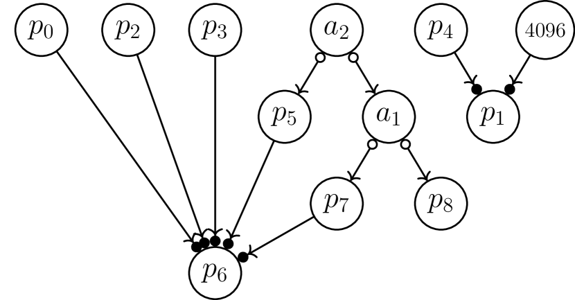
Figure 2: Equations from our example in Fig. 1 and the associated TFG.

A TFG can also include nodes for constants, used to express invariant statements on the markings of the form $p+q=k$. To this end, we assume that we have a family of disjoint sets $K(n)$ for each $n$ in $\mathbb{N}$, such that the “valuation” of a node $v\in K(n)$ is always $n$. We use $K$ to denote the set of all constants.

Definition 4.1 (Token Flow Graph).

A TFG with set of places $P$ is a directed graph $(P,S,R^{\bullet},A^{\circ})$ such that:

• $V=P\cup S$ is a set of vertices (or nodes) with $S\subset K$ a finite set of constants,

• $R^{\bullet}\in V\times V$ is a set of redundancy arcs, $v\mathbin{{\rightarrow}\!{\bullet}}v^{\prime}$,

• $A^{\circ}\in V\times V$ is a set of agglomeration arcs, $v\mathbin{{\circ}\!{\rightarrow}}v^{\prime}$, disjoint from $R$.

The main source of complexity in this approach arises from the need to manage interdependencies between $A^{\circ}$ and $R^{\bullet}$ arcs, that is situations where redundancies and agglomerations are combined. This is not something that can be easily achieved by looking only at the equations in $E$ and thus motivates the need for a specific data structure.

We define several notations that will be useful in the following. We use the notation $v\rightarrow v^{\prime}$ when we have $(v\mathbin{{\rightarrow}\!{\bullet}}v^{\prime})$ or $(v\mathbin{{\circ}\!{\rightarrow}}v^{\prime})$. We say that a node $v$ is a root if it is not the target of an arc. A sequence of nodes $(v_{1},\dots,v_{n})$ in $V^{n}$ is a path if for all $1\leqslant i<n$ we have $v_{i}\rightarrow v_{i+1}$. We use the notation $v\rightarrow^{\star}v^{\prime}$ when there is a path from $v$ to $v^{\prime}$ in the graph, or when $v=v^{\prime}$. We write $v\mathbin{{\circ}\!{\rightarrow}}X$ when $X$ is the largest subset $\{v_{1},\dots,v_{k}\}$ of $V$ such that $X\neq\emptyset$ and $v\mathbin{{\circ}\!{\rightarrow}}v_{i}$ for all $i\in 1..k$. And similarly with reductions, $X\mathbin{{\rightarrow}\!{\bullet}}v$. Finally, the notation $\mathord{\downarrow}{v}$ denotes the set of successors of $v$, that is: $\mathord{\downarrow}{v}\triangleq\{v^{\prime}\in V\setminus\{v\}\,\mid\,v\rightarrow^{\star}v^{\prime}\}$. We extend it to a set of variables $X$ with $\mathord{\downarrow}{X}=\bigcup_{x\in X}\mathord{\downarrow}{x}$.

We display an example of TFG in Fig. 2 (right), which corresponds to the reduction equations generated on our running example, where annotations R and A indicate if an equation is a redundancy or an agglomeration. TFGs were initially defined in [ADZLB21, ADLB22] to efficiently compute the set of concurrent places in a net, that is all pairs of places that can be marked simultaneously in some reachable marking. We reuse this concept here to project reachability formulas.

High Literal Factor.

The projection procedure, described next, applies to cubes only, meaning a conjunction of literals $\bigwedge_{i\in 1..n}\alpha_{i}$. Given a formula $F_{1}$, assumed in DNF, we can apply the projection procedure to each of its cubes, separately. Then the projection of $F_{1}$ is the disjunction of the projected cubes. We assume from now on that $F_{1}$ is a cube formula.

We assume that every literal is in normal form, $\alpha_{i}\triangleq(\sum_{p_{j}\in\mathit{B}}k^{i}_{j}\,p_{j})+b_{i}\geqslant 0$, where the $k^{i}_{j}$’s and $b_{i}$ are in $\mathbb{Z}$. In the following, we denote $\alpha_{i}(q)$ the coefficient associated with variable $q$ in $\alpha_{i}$. We also use $\max_{X}\alpha_{i}$ and $\min_{X}\alpha_{i}$ for the maximal (resp. minimal) coefficient associated with variables in $X\subseteq\mathit{B}$.

$$\alpha_{i}\ =\ \sum_{p\in\mathit{B}}\alpha_{i}(p)\,p+b_{i}\qquad\text{and}\qquad{\textstyle\max_{X}}\,\alpha_{i}\ =\ \max\ \left\{\alpha_{i}(p)\mid p\in X\right\}$$

We define the Highest Literal Factor (HLF) of a set of variables $X$ with respect to a set of normalized literals $(\alpha_{i})_{i\in I}$. In the simplest case, the HLF of $X$ with respect to a single literal, $\alpha$, is the subset of variables in $X$ with the highest coefficients in $\alpha$. Then, the HLF of $X$ with respect to a set of literals is the (possibly empty) intersection of the HLFs of $X$ with respect to each literal. When non-empty, it means that at least one variable in $X$ always has the highest coefficient, and we say then that the whole set $X$ is polarized with respect to the literals $(\alpha_{i})$.

$$\begin{split}\mathrm{HLF}_{X}({\alpha_{i}})&=\ \left\{p\in X\mid\alpha_{i}(p)={\textstyle\max_{X}}\,\alpha_{i}\right\}\\ \mathrm{HLF}_{X}({\alpha_{i}})_{i\in I}&=\ \bigcap_{i\in I}\mathrm{HLF}_{X}({\alpha_{i}})\end{split}$$

Definition 4.2 (Polarized Set of Constraints).

A set of variables $X\subseteq\mathsf{fv}({\mathit{C}})$ is said polarized with respect to a set of normalized literals $\mathit{C}$ when$\mathrm{HLF}_{X}({\mathit{C}})\neq\emptyset$.

We prove in the next section that our procedure is exact when the variables we eliminate are polarized. While this condition seems very restrictive, we observe that it is often true with the queries used in our experiments.

Example.

Let us illustrate our approach with two examples. Assume we want to eliminate an agglomeration $a\mathbin{{\circ}\!{\rightarrow}}\{q,r\}$, meaning that we have the condition $a=q+r$ and that both $q$ and $r$ must disappear. We consider two examples of systems, each with only two literals, and with free variables $\{p,q\}$.

In the left example, the set $\{q,r\}$ is polarized with respect to the initial system (top), with the highest literal factor being $q$. So we replace $q$ with $a$ in both literals and eliminate $r$. Uninvolved variables (the singleton $\{p\}$ in this case) are left unchanged. We can prove that both systems, before and after substitution, are equivalent. For instance, every solution in the resulting system can be associated with a solution of the initial one by taking $q=a$ and $r=0$.

The initial system on the right (top) is non-polarized: the HLF relative to $\{q,r\}$ is $\{q\}$ for the first literal ($+2\,q$ versus $-r$) and $\{r\}$ in the second ($+q$ versus $2\,r$). So we substitute $a$ to the variable with the lowest literal factor, in each literal, and remove the other variable ($r$ in the first literal and $q$ in the second). This is sound because we take into account the worst case in each case. But this is not complete, because we may be too pessimistic. For instance, the resulting system has no solution for $p=2$; because it entails $a\leqslant 6$ and $a\geqslant 7$. But $p=2,q=3,r=2$ is a model of the initial system.

Next, we give a formal description of our projection procedure as a sequence of formula rewriting steps and prove that the result is exact (we have $F_{2}\mathop{\equiv_{E}\,}F_{1}$) when all the reduction steps corresponding to an agglomeration are on polarized variables.

5 Formal Procedure and Proof of Correctness

In all the results of this section, we assume that $N_{1}$ and $N_{2}$ are two nets, with respective sets of places $P_{1},P_{2}$ and initial markings $m_{1},m_{2}$, such that $(N_{1},m_{1})\equiv_{E}(N_{2},m_{2})$. Given a formula $F_{1}$ with support on $N_{1}$, we describe a procedure to project formula $E\land F_{1}$ into a new formula, $F_{2}$, with support on $N_{2}$. Our projection will always lead to a sound formula, meaning $F_{2}\mathop{\sqsubseteq_{E}}F_{1}$. It is also able in many cases (see some statistics in Sect. 6) to result in an exact formula, such that $F_{2}\mathop{\equiv_{E}\,}F_{1}$.

Constraints on TFGs.

To ensure that a TFG preserves the semantics of the system $E$ we must introduce a set of constraints on it. A well-formed TFG $G$ built from $E$ is a graph with one node for every variable and constant occurring in $E$, such that we can find one set of arcs, either $X\mathbin{{\rightarrow}\!{\bullet}}v$ or $v\mathbin{{\circ}\!{\rightarrow}}X$, for every equation of the form $v=\sum_{v_{i}\in X}v_{i}$ in $E$. We deal with inequalities by adding slack variables. We also impose additional constraints which reflect that the same place cannot be removed more than once. Note that the places of $N_{2}$ are exactly the root of $G$ (if we forget about constants).

Definition 5.1 (Well-formed TFG).

A TFG $G=(P,S,R^{\bullet},A^{\circ})$ for the equivalence statement $(N_{1},m_{1})\mathop{\equiv_{E}\,}(N_{2},m_{2})$ is well-formed when the following constraints are met, with $P_{1},P_{2}$ the set of places in $N_{1},N_{2}$:

(T1)

nodes in $S$ are roots: if $v\in S$ then $v$ is a root of $G$;

(T2)

nodes can be removed only once: it is not possible to have $v\mathbin{{\circ}\!{\rightarrow}}w$ and $v^{\prime}\rightarrow w$ with $v\neq v^{\prime}$, or to have both $v\mathbin{{\rightarrow}\!{\bullet}}w$ and $v\mathbin{{\circ}\!{\rightarrow}}w$;

(T3)

$G$ contains all and only the equations in $E$: we have $v\mathbin{{\circ}\!{\rightarrow}}X$ or $X\mathbin{{\rightarrow}\!{\bullet}}v$ if and only if the equation $v=\sum_{v_{i}\in X}v_{i}$ is in $E$;

(T4)

$G$ is acyclic and roots in $P\setminus S$ are exactly the set $P_{2}$.

Given a relation $(N_{1},m_{1})\mathop{\equiv_{E}\,}(N_{2},m_{2})$, the well-formedness conditions are enough to ensure the unicity of a TFG (up-to the choice of constant nodes) when we set each equation to be either in $A$ or in $R$. In this case, we denote the graph $\mathrm{T}({E})$. In practice, we use the tool Reduce [LC23] to generate the reduction system $E$.

Formula Rewriting.

We assume given a relation $(N_{1},m_{1})\equiv_{E}(N_{2},m_{2})$, and its associated well-formed TFG written $\mathrm{T}({E})$. We consider that $F_{1}$ is a cube of $n$ literals, $F_{1}\triangleq\bigwedge_{i\in 1..n}\alpha^{0}_{i}$. Our algorithm rewrites each $\alpha^{0}_{i}$ by applying iteratively an elimination step, described next, according to the constraints expressed in $\mathrm{T}({E})$. The final result is a conjunction $F_{2}=\bigwedge_{i\in 1..n}\beta_{i}$, where each literal $\beta_{i}$ has support in $N_{2}$. Rewriting can only replace a variable with a group of other variables that are its predecessors in the TFG, which ensures termination in polynomial time (in the size of $E$). Although the result has the same number of literals, it usually contains many redundancies and trivial constant comparisons, so that, after simplification, $F_{2}$ can actually be much smaller than $F_{1}$.

A reduction step (to be applied repeatedly) takes as input the current set of literals, $\mathit{C}=(\alpha_{i})_{i\in 1..n}$, and modifies it. To ease the presentation, we also keep track of a set of variables, $\mathit{B}$ such that $\bigcup_{i\in 1..n}\mathsf{fv}({\alpha_{i}})\subseteq\mathit{B}$.

An elimination step is a reduction written $(\mathit{B},\mathit{C})\mapsto(\mathit{B}^{\prime},\mathit{C}^{\prime})$ where $\mathit{C}=(\alpha_{i})_{i\in 1..n}$ and $\mathit{B}^{\prime}\subsetneq\mathit{B}$, defined as one of the three cases below (one for redundancy, and two for agglomerations, depending on whether the removed variables are polarized or not). We assume that literals are in normal form and that $X$ is a set of variables $\{x_{1},\dots,x_{k}\}$. Note the precondition $\mathord{\downarrow}{X}\cap B=\emptyset$ on all rules, which forces them to be applied bottom-up on the TFG (remember it is a DAG). We gave a short example of how to apply rules (AGP) and (AGD) at the end of the previous section.

(RED)

If $X\mathbin{{\rightarrow}\!{\bullet}}p$ and $\mathord{\downarrow}{p}\cap B=\emptyset$ then $(\mathit{B},\mathit{C})\mapsto(\mathit{B}^{\prime},\mathit{C}^{\prime})$ holds, where $\mathit{B}^{\prime}=\mathit{B}\setminus\{p\}$ and $\mathit{C}^{\prime}$ is the set of literals $\alpha^{\prime}_{i}$ obtained by normalizing the linear constraint $\alpha_{i}\{p\leftarrow x_{1}+\dots+x_{k}\}$. That is, we substitute $p$ with $\sum_{x_{i}\in X}x_{i}$ in $\mathit{C}$, which is the meaning of the redundancy equation (constraint (T3) in Def. 5.1).

(AGP)

If $a\mathbin{{\circ}\!{\rightarrow}}X$ with $\mathord{\downarrow}{X}\cap B=\emptyset$, $a\in\mathit{B}$, and $X$ polarized with respect to $\mathit{C}$. Then $(\mathit{B},\mathit{C})\mapsto(\mathit{B}^{\prime},\mathit{C}^{\prime})$ holds, where $\mathit{B}^{\prime}=\mathit{B}\setminus X$, and, by taking $x_{j}\in\mathrm{HLF}_{X}({\mathit{C}})$, we define $\mathit{C}^{\prime}$ as the set of literals $\alpha^{\prime}_{i}$ obtained by normalizing the linear constraint $\alpha_{i}\{x_{l}\leftarrow 0\}_{l\neq j}\{x_{j}\leftarrow a\}$. That is, we eliminate the variables $x_{l}$, different from $x_{j}$, from $\mathit{C}$ and replace $x_{j}$ with $a$; where $x_{j}$ is a variable of $X$ that always have the highest coefficient in each literal (among the ones of $X$).

(AGD)

If $a\mathbin{{\circ}\!{\rightarrow}}X$ with $\mathord{\downarrow}{X}\cap B=\emptyset$, $a\in\mathit{B}$, and $X$ is not polarized with respect to $\mathit{C}$. Then $(\mathit{B},\mathit{C})\mapsto(\mathit{B}^{\prime},\mathit{C}^{\prime})$ holds, where $\mathit{B}^{\prime}=\mathit{B}\setminus X$ and $\mathit{C}^{\prime}$ is the set of literals $\alpha^{\prime}_{i}$ obtained by normalizing the linear constraint $\alpha_{i}\{x_{l}\leftarrow 0\}_{l\neq j}\{x_{j}\leftarrow a\}$ such that $\alpha_{i}(x_{j})=\min_{X}\alpha_{i}$. Meaning we eliminate the variables $x_{l}$ different from $x_{j}$ from $\alpha_{i}$ and replace $x_{j}$ with $a$, where $x_{j}$ is a variable with the smallest coefficient in $\alpha_{i}$ (among the ones of $X$). Note that the chosen variable $x_{j}$ is not necessarily the same in every literal of $\mathit{C}$.

Our goal is to preserve the semantics of formulas at each reduction step, in the sense of the relations $\mathop{\sqsubseteq_{E}}$ and $\mathop{\equiv_{E}\,}$. In the following, we use $\mathit{C}$ to represent both a set of literals $(\alpha_{i})_{i\in I}$ and the cube formula $\bigwedge_{i\in I}\alpha_{i}$. We can prove that the elimination steps corresponding to the redundancy (RED) and polarized agglomeration (AGP) cases preserve the semantics of the formula $\mathit{C}$. On the other hand, a non-polarized agglomeration step (AGD) may lose some markings.

Proof of the Algorithm.

We prove the main result of the paper, namely that fast quantifier elimination preserves the integer solutions of a system when we only have polarized agglomerations. To this end, we need to prove two theorems. First, Theorem 5.1, which entails the soundness of one step of elimination. It also entails completeness for rules (RED) and (AGP). Second, we prove a progress property (Th. 5.4 below), which guarantees that we can apply elimination steps until we reach a set of literals $C^{\prime}$ with support on the reduced net $N_{2}$.

Theorem 5.1 (Projection Equivalence).

If $(\mathit{B},\mathit{C})\mapsto(\mathit{B}^{\prime},\mathit{C}^{\prime})$ is a (RED) or (AGP) reduction then $\mathit{C}^{\prime}\mathop{\equiv_{E}\,}\mathit{C}$; otherwise $\mathit{C}^{\prime}\mathop{\sqsubseteq_{E}}\mathit{C}$.

We prove Th. 5.1 in two steps. We start by proving that elimination steps are sound, meaning that the integer solutions of $\mathit{C}^{\prime}$ are also solutions of $\mathit{C}$ (up-to $E$). Then we prove that elimination is also complete for rules (RED) and (AGP). In the following, we use $\mathit{C}$ to represent both a set of literals $(\alpha_{i})_{i\in I}$ and the cube formula $\bigwedge_{i\in I}\alpha_{i}$.

Lemma 5.2 (Soundness).

If $(\mathit{B},\mathit{C})\mapsto(\mathit{B}^{\prime},\mathit{C}^{\prime})$ then $\mathit{C}^{\prime}\mathop{\sqsubseteq_{E}}\mathit{C}$.

Proof.

Take a valuation $m^{\prime}$ of $\mathbb{N}^{\mathit{B}^{\prime}}$ such that $m^{\prime}\models E\land\mathit{C}^{\prime}$. We want to show that there exists a marking $m$ of $\mathbb{N}^{\mathit{B}}$ such that $m\mathop{\equiv_{E}\,}m^{\prime}$ satisfying $E\land\mathit{C}$.

We have three possible cases, corresponding to rule (RED), (AGP) or (AGD). In each case, we provide a marking $m$ built from $m^{\prime}$. Since $m\mathop{\equiv_{E}\,}m^{\prime}$ is enough to prove $m\models E$, we only need to check two properties: first that $m\mathop{\equiv_{E}\,}m^{\prime}$ ($\ast$), then that $m\models\alpha$ for every literal $\alpha$ in $\mathit{C}$ ($\ast\ast$).

(RED)

In this case we have $X\mathbin{{\rightarrow}\!{\bullet}}p$ and $\mathit{B}^{\prime}=\mathit{B}\setminus\{p\}$, with $X=\{x_{1},\dots,x_{k}\}$. We can extend $m^{\prime}$ into the unique valuation $m$ of $\mathbb{N}^{\mathit{B}}$ such that $m(p)=m^{\prime}(x_{1})+\dots+m^{\prime}(x_{k})$ and $m(v)=m^{\prime}(v)$ for all other nodes $v$ in $\mathit{B}\setminus\{p\}$. Since $p=x_{1}+\dots+x_{k}$ is an equation of $E$ (condition (T3)) we obtain that $m^{\prime}\mathop{\equiv_{E}\,}m$ and therefore also $m\models E$ ($\ast$).

We now prove that $m\models\mathit{C}$. The literals in $\mathit{C}^{\prime}$ are of the form $\alpha\sigma$ with $\sigma$ the substitution $\{p\leftarrow x_{1}+\dots+x_{k}\}$ and $\alpha$ in $\mathit{C}$. Remember that, with our notations (e.g. Equation (1) in page 1), we have $m\models\alpha$ if and only if $\alpha\{m\}$ SAT (is satisfiable). By hypothesis, $m^{\prime}\models\alpha\sigma$. Hence, $\alpha\sigma\{m^{\prime}\}$ SAT, which is equivalent to $\alpha\{m\}$ SAT, and therefore $m\models\alpha$ ($\ast\ast$), as required.

(AGP)

In this case we have $a\mathbin{{\circ}\!{\rightarrow}}X$ with $X=\{x_{1},\dots,x_{k}\}$, polarized relative to $\mathit{C}$, and $B^{\prime}=B\setminus X$. We consider $x_{j}$ in $X$ the variable in $\mathrm{HLF}_{X}({\mathit{C}})$ that was chosen in the reduction; meaning that $\mathit{C}^{\prime}$ is a conjunction of literals of the form $\alpha\{x_{l}\leftarrow 0\}_{l\neq j}\{x_{j}\leftarrow a\}$, with $\alpha$ a literal of $\mathit{C}$. Given $m^{\prime}$ a model of $\mathit{C}^{\prime}$, we define $m$ the unique marking on $\mathbb{N}^{\mathit{B}}$ such that $m(x_{j})=m(a)$, $m(x_{l})=0$ for all $l\neq j$, and $m(v)=m^{\prime}(v)$ for all other variables $v$ in $B\setminus X$.

From Lemma 2 of [ADZLB21] (the “token propagation” property of TFGs), we know that any distribution of $m(a)$ tokens, in place $a$, over the $(x_{i})_{i\in 1..k}$, is also a model of $E$. Which means that $m\models E$ $(\ast)$. Note that the token propagation Lemma does not imply that the value of $m(v)$, for the nodes “below $X$” ($v$ in $\mathord{\downarrow}{X}$), is unchanged. This is not problematic, since the side condition $\mathord{\downarrow}{X}\cap\mathit{B}=\emptyset$ ensures that these nodes are not in $\mathit{B}$, and therefore cannot influence the value of $\alpha\{m\}$.

Consider a literal $\alpha$ in $\mathit{C}$. Since $m^{\prime}\models\mathit{C}^{\prime}$, we have that $\alpha\{x_{l}\leftarrow 0\}_{l\neq j}\{x_{j}\leftarrow a\}\{m^{\prime}\}$ SAT, which is exactly $\alpha\{m\}$, since $\mathord{\downarrow}{X}\cap B=\emptyset$, as needed ($\ast\ast$).

(AGD)

In this case we have $a\mathbin{{\circ}\!{\rightarrow}}X$ with $X=\{x_{1},\dots,x_{k}\}$, non-polarized relative to $\mathit{C}$, and $B^{\prime}=B\setminus X$. We know that $m^{\prime}\models E$, therefore there is a marking $m$ of $\mathbb{N}^{\mathit{B}}$ that extends $m^{\prime}$ such that $m\mathop{\equiv_{E}\,}m^{\prime}$ ($\ast$).

Consider a literal $\alpha$ in $\mathit{C}$. By definition of (AGD), we have an associated literal $\alpha^{\prime}\triangleq\alpha\{x_{l}\leftarrow 0\}_{l\neq j}\{x_{j}\leftarrow a\}$ in $\mathit{C}^{\prime}$ such that $\alpha(x_{j})=\min_{X}\alpha_{i}$. Since the coefficient of $x_{j}$ is minimal, we have that $\sum_{i\in 1..k}\alpha(x_{i})\,m(x_{i})\geqslant\alpha(x_{j})\,\sum_{i\in 1..k}m(x_{i})=\alpha(x_{j})\,m^{\prime}(a)$, and therefore $\sum_{v\in\mathit{B}}\alpha(v)\,m(v)\geqslant\sum_{v\in\mathit{B}^{\prime}}\alpha^{\prime}(v)\,m^{\prime}(v)$. The result follows from the fact that $\alpha\{m\}$ SAT ($\ast\ast$).

∎∎

Now we prove that our quantifier elimination step, for the (RED) and (AGP) cases, leads to a complete projection, that is any solution of the initial formula corresponds to a projected solution in the projected formula.

Lemma 5.3 (Completeness).

If $(\mathit{B},\mathit{C})\mapsto(\mathit{B}^{\prime},\mathit{C}^{\prime})$ is a (RED) or (AGP) reduction then $\mathit{C}\mathop{\sqsubseteq_{E}}\mathit{C}^{\prime}$.

Proof.

Take a marking $m$ of $\mathbb{N}^{\mathit{B}}$ such that $m\models E\land\mathit{C}$. We want to show that there exists a valuation $m^{\prime}$ of $\mathbb{N}^{\mathit{B}^{\prime}}$ such that $m\mathop{\equiv_{E}\,}m^{\prime}$ ($\ast$) and $m^{\prime}\models\mathit{C}^{\prime}$ ($\ast\ast$). This is enough to prove $m^{\prime}\models E\land C^{\prime}$. We have two different cases, corresponding to the rules (RED) and (AGP).

(RED)

In this case we have $X\mathbin{{\rightarrow}\!{\bullet}}p$ with $X=\{x_{1},\dots,x_{k}\}$ and $B^{\prime}=B\setminus\{p\}$. We define $m^{\prime}$ as the (unique) projection of $m$ on $\mathit{B}^{\prime}$. Since $m\models E$ we have that $m^{\prime}\mathop{\equiv_{E}\,}m$ ($\ast$).

Also, literals in $\mathit{C}^{\prime}$ are of the form $\alpha^{\prime}\triangleq\alpha\{p\leftarrow x_{1}+\dots+x_{k}\}$ where $\alpha$ is a literal of $\mathit{C}$. Since $m(p)=\sum_{i\in 1..k}m(x_{i})$ and $m$ is a model of $\alpha$, it is also the case that $m^{\prime}$ is a model of $\alpha^{\prime}$ $(\ast\ast)$.

(AGP)

In this case we have $a\mathbin{{\circ}\!{\rightarrow}}X$ with $X=\{x_{1},\dots,x_{k}\}$ and $\mathit{B}^{\prime}=B\setminus X$. We define $m^{\prime}$ as the (unique) projection of $m$ on $\mathit{B}^{\prime}$, by taking $m^{\prime}(a)=\sum_{i\in 1..k}m(x_{i})$. Since $m\models E$ we have that $m^{\prime}\mathop{\equiv_{E}\,}m$ ($\ast$).

We consider $x_{j}$ in $X$ the variable in $\mathrm{HLF}_{X}({\mathit{C}})$ that was chosen in the reduction; meaning that $\mathit{C}^{\prime}$ is a conjunction of literals of the form $\alpha\{x_{l}\leftarrow 0\}_{l\neq j}\{x_{j}\leftarrow a\}$, with $\alpha$ a literal of $\mathit{C}$. Since $\sum_{i\in 1..k}\alpha(x_{i})\,m(x_{i})\leqslant\alpha(x_{j})\,\sum_{i\in 1..k}m(x_{i})=\alpha(x_{j})\,m^{\prime}(a)$, we have $m^{\prime}$ is a model of $\alpha^{\prime}$ ($\ast\ast$).∎

∎

The final step of our proof relies on a progress property, meaning there is always a reduction step to apply except when all the literals have their support on the reduced net, $N_{2}$. This property relies on relation $\mapsto^{*}$, which is the transitive closure of $\mapsto$. Together with Th. 5.1, the progress theorem ensures the existence of a sequence $(P,\mathit{C})\mapsto^{*}(P_{2},\mathit{C}^{\prime})$, such that $C\mathop{\equiv_{E}\,}C^{\prime}$ (or $C^{\prime}\mathop{\sqsubseteq_{E}}C$ if we have at least one non-polarized agglomeration). In this context, $P$ is the set of all variables occurring in the TFG of $E$, and therefore it contains $P_{1}\cup P_{2}$.

Theorem 5.4 (Progress).

Assume $(P,F_{1})\mapsto^{*}(\mathit{B},\mathit{C})$ then either $\mathit{B}\subseteq P_{2}$, the set of places of $N_{2}$, or there is an elimination step $(\mathit{B},\mathit{C})\mapsto(\mathit{B}^{\prime},\mathit{C}^{\prime})$ such that $\mathsf{fv}({\mathit{C}^{\prime}})\subseteq\mathit{B}^{\prime}$ and the places removed from $B$ have no successors in $\mathit{B}^{\prime}$: for all places $p$ in $\mathit{B}\setminus\mathit{B}^{\prime}$, we have $\mathord{\downarrow}{p}\cap\mathit{B}=\emptyset$.

Proof.

Assume we have $(P,F_{1})\mapsto^{*}(\mathit{B},\mathit{C})$ and $\mathit{B}\nsubseteq P_{2}$.

By condition (T4) in Def. 5.1, we know that $P_{2}$ are roots in the TFG $\mathrm{T}({E})$. We consider the set of nodes in $B\setminus P_{2}$, which corresponds to nodes in $B$ with at least one parent. Also, by condition (T4), we know that $\mathrm{T}({E})$ is acyclic, then there are nodes in $\mathit{B}\setminus P_{2}$ that have no successors in $\mathit{B}$. We call this set $L$. Hence, $L\triangleq\{v\mid v\in\mathit{B}\setminus P_{2}\land\mathord{\downarrow}{v}\cap B=\emptyset\}$.

Take a node $p$ in $L$. We have two possible cases. If there is a set $X$ such that $X\mathbin{{\rightarrow}\!{\bullet}}p$, we can apply the (RED) elimination rule. Otherwise, there exists a node $a$ and a set $X\subseteq L$ (by condition (T2)) such that $a\mathbin{{\circ}\!{\rightarrow}}X$ with $p\in X$. In this case, apply rule (AGP) or (AGD), depending on whether the agglomeration is polarized or not.∎∎

Remark. We have designed the rule (AGD) to obtain at least $F_{2}\mathop{\sqsubseteq_{E}}F_{1}$ when the procedure is not complete (instead of $F_{2}\mathop{\equiv_{E}\,}F_{1}$), which is useful for finding witnesses (see Th. 3.1). Alternatively, we could propose a variant rule, say (AGD’), which chooses the variable $x_{j}$ having the highest coefficient in $\alpha_{i}$, that is $\alpha_{i}(x_{j})=\max_{X}\alpha_{i}$. This variant guarantees a dual result, that is $F_{1}\mathop{\sqsubseteq_{E}}F_{2}$. In this case, if $F_{2}$ is not reachable then $F_{1}$ is not reachable, which is useful to prove invariants.

6 Experimental Results

Data-Availability Statement.

We have implemented our fast quantifier elimination procedure in a new, open-source tool called Octant [Ama23], available on GitHub. All the tools, scripts and benchmarks used in our experiments are part of our artifact [ADZLB23a].

We use an extensive, and independently managed, set of models and formulas collected from the 2022 edition of the Model Checking Contest (MCC) [KBG⁺22]. The benchmark is built from a collection of $128$ models. Most models are parametrized and can have several instances. This amounts to about $1\,400$ different instances of Petri nets whose size varies widely, from $9$ to $50\,000$ places, and from $7$ to $200\,000$ transitions. This collection provides a large number of examples with various structural and behavioral characteristics, covering a large variety of use cases. Each year, the MCC organizers randomly generate $16$ reachability formulas for each instance. The pair of a Petri instance and a formula is a query; which means we have more than $22\,000$ queries overall.

We do not compute reductions ourselves but rely on the tool Reduce, part of the latest public release of Tina [LC23]. We define the reduction ratio ($r_{p}$) of an instance as the ratio $(p_{init}-p_{red})/p_{init}$ between the number of places before ($p_{init}$) and after ($p_{red}$) reduction. We only consider instances with a ratio, $r_{p}$, between $1\%$ and $100\%$ (meaning the net is fully reduced), which still leaves about $17\,000$ queries, so about $77\%$ of the whole benchmark. More information about the distribution of reductions can be found in [ABD22, BLBDZ19], where we show that almost half the instances ($48\%$) can be reduced by a factor of $25\%$ or more.

The size of the reduction system, $E$, is proportional to the number of places that can be removed. To give a rough idea, the mean number of variables in $E$ is $1\,375$, with a median value of $114$ and a maximum of about $62\,000$. The number of literals is also rather substantial: a mean of $869$ literals ($62\%$ of agglomerations and $38\%$ of redundancies), with a median of $27$ and a maximum of about $38\,000$.

We report on the results obtained on two main categories of experiments: first with model-checking, to evaluate if our approach is effective in practice, using real tools; then to assess the precision and performance of our fast quantifier elimination procedure.

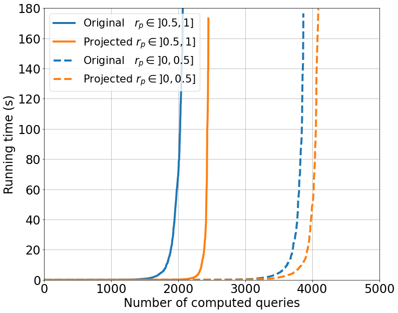
Figure 3: Random walk w/wo reductions.

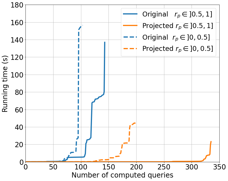
Figure 4: $k$-induction w/wo reductions.

Model-Checking.

We start by showing the effectiveness of our approach on both $k$-induction and random walk. This is achieved by comparing the computation time, with and without reductions, on a model-checker that provides a “reference” implementation of these techniques. (Without any other optimizations that could interfere with our experiments.) It is interesting to test the results of our optimization separately on these two techniques. Indeed, each technique is adapted to a different category of queries: properties that can be decided by finding a witness, meaning true EF formulas or false AG ones, can often be checked more efficiently using a random exploration of the state space. On the other hand, symbolic verification methods are required when we want to check invariants.

We display our results using the two “cactus plots” in Figs. 4 and 4. We distinguish between two categories of instances, depending on their reduction ratio. We use dashed lines for models with a low or moderate reduction ratio (value of $r_{p}$ less than $50\%$) and solid lines for models that can be reduced by more than half. The first category amounts to roughly $10\,700$ queries ($62\%$ of our benchmark), while the second category contains about $6\,000$ queries. The most interesting conclusion we can draw from these results is the fact that our approach is beneficial even when there is only a limited amount of reductions.

Our experiments were performed with a maximal timeout of $180\text{\,}\mathrm{s}$ and integrated the projection time into the total execution time. The “vertical asymptote” that we observe in these plots is a good indication that we cannot expect further gains, without projection, for timeout values above 60s. Hence, our choice of timeout value does not have an overriding effect. We observe moderate performance gains with random exploration (with $\times 1.06$ more computed queries on low-reduction instances and $\times 1.19$ otherwise) and good results with $k$-induction (respectively $\times 1.94$ and $\times 2.33$).

We obtain better results if we focus on queries that take more than $1\text{\,}\mathrm{s}$ on the original formula, which indicates that reductions are most effective on “difficult problems” (there is not much to gain on instances that are already easy to solve). With random walk, for instance, the gain becomes $\times 1.48$ for low-reduction instances and $\times 1.93$ otherwise. The same observation is true with $k$-induction, with performance gains of $\times 3.78$ and $\times 3.51$ respectively.

Model-Checking under Real Conditions.

We also tested our approach by transparently adding polyhedral reductions as a front-end to three different model-checkers: TAPAAL [DJJ⁺12], ITS [TM15], and LoLA [Wol18], that implement portfolios of verification techniques. All three tools regularly compete in the MCC (on the same set of queries that we use for our benchmark), TAPAAL and ITS share the top two places in the reachability category of the 2022 and 2023 editions.

We ran each tool on our set of complete projections, which amounts to almost $100\,000$ runs (one run for each tool, once on both the original and the projected query). We obtained a $100\%$ reliability result, meaning that all tools gave compatible results on all the queries; and therefore also compatible results on the original and the projected formulas.

A large part of the queries can be computed by all the tools in less than $100\text{\,}\mathrm{ms}$ and can be considered as easy. These queries are useful for testing reliability but can skew the interpretation of results when comparing performances. This is why we decided to focus our results on a set of $809$ challenging queries, that we define as queries for which either TAPAAL or ITS, or both, are not able to compute a result before projection. The $809$ challenging queries ($4\%$ of queries) are well distributed, since they cover $209$ different instances ($14\%$ of all instances), themselves covering $43$ different models ($33\%$ of the models).

We display the results obtained on the challenging queries, for a timeout of $180\text{\,}\mathrm{s}$, in Table 5. We provide the number of computed queries before and after projection, together with the mean and median speed-up (the ratio between the computation time with and without projection). The “Exclusive” column reports, for each tool, the number of queries that can only be computed using the projected formula. Note that we may sometimes time out with the projected query, but obtain a result without. This can be explained by cases where the size of the formula blows up during the transformation into DNF.

Tool	# Queries			Speed-up			# Excl. Queries
	Original	Projected		Mean	Median
ITS	$302$	$352$		$1.42$	$1.00$		$78$
LoLA	$143$	$205$		$14.97$	$1.44$		$76$
TAPAAL	$134$	$216$		$1.87$	$1.17$		$99$

Figure 5: Impact of projections on the challenging queries.

We observe substantial performance gains with our approach and can solve about half of the challenging queries. For instance, we are able to compute $\times 1.6$ more challenging queries with TAPAAL using projections than without. (We display more precise results on TAPAAL, the winner of the MCC 2022 edition, in Fig. 7.) We were also able to compute $62$ queries, using projections, that no tool was able to solve during the last MCC (where each tool has $3\,600\text{\,}\mathrm{s}$ to answer $16$ queries on a given model instance). All these results show that polyhedral reductions are effective on a large set of queries and that their benefits do not significantly overlap with other existing optimizations, an observation that was already made, independently, in [ABD22] and [BDJ⁺19].

The approach implemented in Octant was partially included in the version of our model-checker, called SMPT [AZ23], that participated in the MCC 2023 edition. We mainly left aside the handling of under-approximated queries, when the formula projection is not complete. While SMPT placed third in the reachability category, the proportion of queries it was able to solve raised by $5.5\%$ between 2022 (without the use of Octant) and 2023, to reach a ratio of $93.6\%$ of all queries solved with our tool. A $5\%$ gain is a substantial result, taking into account that the best-performing tools are within $1\%$ of each other; the ratios for ITS and TAPAAL in 2023 are respectively $94.6\%$ and $94.3\%$.

Performance of Fast Elimination.

Our last set of experiments is concerned with the accuracy and performance of our quantifier elimination procedure. We decided to compare our approach with Redlog [DS97] and isl [Ver10] (we give more details on these two tools in Sect. 7).

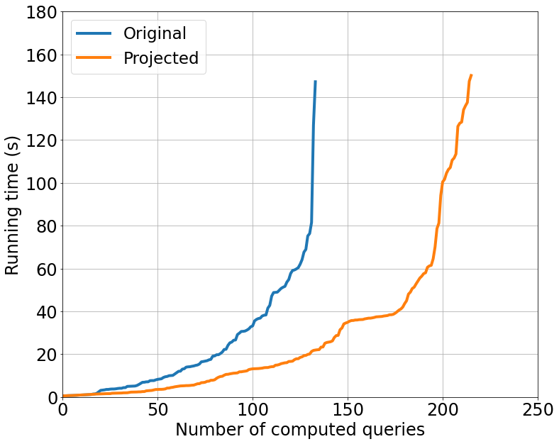
Figure 6: TAPAAL w/wo polyhedral reductions.

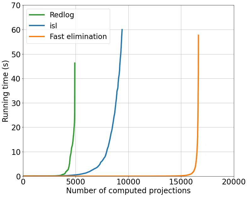
Figure 7: Redlog vs isl vs Fast elimination.

We display our results in the cactus plot of Fig. 7, where we compare the number of projections we can compute given a fixed timeout. We observe a significant performance gap. For instance, with a timeout of $60\text{\,}\mathrm{s}$, we are able to compute $16\,653$ projections, out of $16\,976$ queries ($98\%$), compared to $9\,407$ ($55\%$) with isl or $4\,915$ ($29\%$) with Redlog. So an increase of $\times 1.77$ over the better of the two tools. This provides more empirical evidence that the class of linear systems we manage is not trivial, or at least does not correspond to an easy case for the classical procedure implemented in Redlog and isl. We also have good results concerning the precision of our approach, since we observe that about $80\%$ of the projections are complete. Furthermore, projections are inexpensive. For instance, the computation time is less than $1\text{\,}\mathrm{s}$ for $96\%$ of the formulas. We also obtained a median reduction ratio (computed as for the number of places) of $0.2$ for the number of cubes and their respective number of literals.

7 Discussion and Related Works

We proposed a quantifier elimination procedure that can take benefit of polyhedral reductions and can be used, transparently, as a pre-processing step of existing model-checkers. The main characteristic of our approach is to rely on a graph structure, called Token Flow Graph, that encodes the specific shape of our reduction equations.

The idea of using linear equations to keep track of the effects of structural reductions originates from [BLBDZ18, BLBDZ19], as a method for counting the number of reachable markings. We extended this approach to Bounded Model Checking (BMC) in [ABD22] where we defined our polyhedral abstraction equivalence, $\mathop{\equiv_{E}\,}$, and in [ADZLB23b] where we proposed a procedure to automatically prove when such abstractions are correct. The idea to extend this relation to formulas is new (see Def. 3.1). In this paper, we broaden our approach to a larger set of verification methods; most particularly $k$-induction, which is useful to prove invariants, and simulation (or random walk), which is useful for finding counter-examples. We introduced the notion of a Token Flow Graph (TFG) in [ADZLB21], as a new method to compute the concurrent places of a net; meaning all pairs of places that can be marked simultaneously. We find a new use for TFGs here, as the backbone of our variable elimination algorithm, and show that we can efficiently eliminate variables in systems of the form $E\wedge F$, for an arbitrary $F$.

We formulated our method as a variable elimination procedure for a restricted class of linear systems. There exist some well-known classes of linear systems where variable elimination has a low complexity. A celebrated example is given by the link between unimodular matrices and integral polyhedra [HK10], which is related to many examples found in abstract domains used in program verification, such as systems of differences [AS80] or octagon [Min06, JM09]. To the best of our knowledge, none of the known classes correspond to what we define using TFGs. There is also a rich literature about quantifier elimination in Presburger arithmetic, such as Cooper’s algorithm [Coo72, Haa18] or the Omega test [Pug91] for instance, and how to implement it efficiently [HLL92, LS07, Mon10]. These algorithms have been implemented in several tools, using many different approaches: automata-based, e.g. TaPAS [LP09]; inside computer algebra systems, like with Redlog [DS97]; or in program analysis tools, like isl [Ver10], part of the Barvinok toolbox. Another solution would have been to retrieve “projected formulas” directly from SMT solvers for linear arithmetic, which often use quantifier elimination internally. Unfortunately, this feature is not available, even though some partial solutions have been proposed recently [BDHP]. All the exact methods that we tested have proved impractical in our case. This was to be expected. Quantifier elimination can be very complex, with an exponential time complexity in the worst case (for existential formulas as we target); it can generate very large formulas; and it is highly sensitive to the number of variables, when our problem often involves several hundreds and sometimes thousands of variables. Also, quantifier elimination often requires the use of a divisibility operator (also called stride format in [Pug91]), which is not part of the logic fragment that we target.

Another set of related works is concerned with polyhedral techniques [FL11], used in program analysis. For instance, our approach obviously shares similarities with works that try to derive linear equalities between variables of a program [CH78], and polyhedral abstractions are very close in spirit to the notion of linear dependence between vectors of integers (markings in our case) computed in compiler optimizations. Another indication of this close relationship is the fact that isl, the numerical library that we use to compare our performances, was developed to support polyhedral compilation. We need to investigate this relationship further and see if our approach could find an application with program verification. From a more theoretical viewpoint, we are also looking into ways to improve the precision of our projection in the cases where we find non-polarized sets of constraints.

References

- [ABB+16] Elvio Gilberto Amparore, Gianfranco Balbo, Marco Beccuti, Susanna Donatelli, and Giuliana Franceschinis. 30 years of GreatSPN. In Principles of Performance and Reliability Modeling and Evaluation. Springer, 2016. doi:10.1007/978-3-319-30599-8_9.
- [ABC+19] Elvio Amparore, Bernard Berthomieu, Gianfranco Ciardo, Silvano Dal Zilio, Francesco Gallà, Lom Messan Hillah, Francis Hulin-Hubard, Peter Gjøl Jensen, Loïg Jezequel, Fabrice Kordon, Didier Le Botlan, Torsten Liebke, Jeroen Meijer, Andrew Miner, Emmanuel Paviot-Adet, Jiří Srba, Yann Thierry-Mieg, Tom van Dijk, and Karsten Wolf. Presentation of the 9th Edition of the Model Checking Contest. In Tools and Algorithms for the Construction and Analysis of Systems (TACAS), LNCS. Springer, 2019. doi:10.1007/978-3-662-58381-4\_9.
- [ABD21] Nicolas Amat, Bernard Berthomieu, and Silvano Dal Zilio. On the Combination of Polyhedral Abstraction and SMT-based Model Checking for Petri nets. In Application and Theory of Petri Nets and Concurrency (Petri Nets), LNCS. Springer, 2021. doi:10.1007/978-3-030-76983-3\_9.
- [ABD22] Nicolas Amat, Bernard Berthomieu, and Silvano Dal Zilio. A Polyhedral Abstraction for Petri Nets and its Application to SMT-Based Model Checking. Fundamenta Informaticae, 187(2-4), 2022. doi:10.3233/FI-222134.
- [ADLB22] Nicolas Amat, Silvano Dal Zilio, and Didier Le Botlan. Leveraging polyhedral reductions for solving Petri net reachability problems. International Journal on Software Tools for Technology Transfer, 25, 2022. doi:10.1007/s10009-022-00694-8.
- [ADZLB21] Nicolas Amat, Silvano Dal Zilio, and Didier Le Botlan. Accelerating the Computation of Dead and Concurrent Places using Reductions. In Model Checking Software (SPIN), LNCS. Springer, 2021. doi:10.1007/978-3-030-84629-9\_3.
- [ADZLB23a] Nicolas Amat, Silvano Dal Zilio, and Didier Le Botlan. Artifact for VMCAI 2024 Paper "Project and Conquer: Fast Quantifier Elimination for Checking Petri Net Reachability", 2023. doi:10.5281/zenodo.7935153.
- [ADZLB23b] Nicolas Amat, Silvano Dal Zilio, and Didier Le Botlan. Automated Polyhedral Abstraction Proving. In Application and Theory of Petri Nets and Concurrency (Petri Nets), LNCS. Springer, 2023. doi:10.1007/978-3-031-33620-1_18.
- [Ama23] Nicolas Amat. Octant (version 1.0): projection of Petri net reachability properties, 2023. URL: https://github.com/nicolasAmat/Octant.
- [AS80] Bengt Aspvall and Yossi Shiloach. A polynomial time algorithm for solving systems of linear inequalities with two variables per inequality. SIAM Journal on computing, 9(4), 1980. doi:10.1137/0209063.
- [AZ23] Nicolas Amat and Silvano Dal Zilio. SMPT: A Testbed for Reachability Methods in Generalized Petri Nets. In Formal Methods (FM), LNCS. Springer, 2023. doi:10.1007/978-3-031-27481-7_25.
- [BDHP] Max Barth, Daniel Dietsch, Matthias Heizmann, and Andreas Podelski. Ultimate Eliminator at SMT-COMP 2022.
- [BDJ+19] Frederik M Bønneland, Jakob Dyhr, Peter G Jensen, Mads Johannsen, and Jiří Srba. Stubborn versus structural reductions for Petri nets. Journal of Logical and Algebraic Methods in Programming, 102, 2019. doi:10.1016/j.jlamp.2018.09.002.
- [Ber87] G. Berthelot. Transformations and Decompositions of Nets. In Petri Nets: Central Models and Their Properties (ACPN), LNCS. Springer, 1987. doi:10.1007/978-3-540-47919-2\_13.
- [BLBDZ18] Bernard Berthomieu, Didier Le Botlan, and Silvano Dal Zilio. Petri net reductions for counting markings. In Model Checking Software (SPIN), LNCS. Springer, 2018. doi:10.1007/978-3-319-94111-0\_4.
- [BLBDZ19] Bernard Berthomieu, Didier Le Botlan, and Silvano Dal Zilio. Counting Petri net markings from reduction equations. International Journal on Software Tools for Technology Transfer, 22, 2019. doi:10.1007/s10009-019-00519-1.
- [BRV04] B. Berthomieu, P.-O. Ribet, and F. Vernadat. The tool TINA – Construction of abstract state spaces for Petri nets and time Petri nets. International Journal of Production Research, 42(14), 2004. doi:10.1080/00207540412331312688.
- [CH78] Patrick Cousot and Nicolas Halbwachs. Automatic discovery of linear restraints among variables of a program. In Proceedings of the 5th ACM SIGACT-SIGPLAN symposium on Principles of programming languages, 1978. doi:10.1145/512760.512770.
- [CJGK+18] Edmund M Clarke Jr, Orna Grumberg, Daniel Kroening, Doron Peled, and Helmut Veith. Model checking. MIT press, 2018.
- [Coo72] David C Cooper. Theorem proving in arithmetic without multiplication. Machine intelligence, 7(91-99), 1972.
- [DJJ+12] Alexandre David, Lasse Jacobsen, Morten Jacobsen, Kenneth Yrke Jørgensen, Mikael H. Møller, and Jiří Srba. TAPAAL 2.0: Integrated Development Environment for Timed-Arc Petri Nets. In Tools and Algorithms for the Construction and Analysis of Systems (TACAS), LNCS. Springer, 2012. doi:10.1007/978-3-642-28756-5_36.
- [DS97] Andreas Dolzmann and Thomas Sturm. Redlog: Computer algebra meets computer logic. ACM Sigsam Bulletin, 31(2), 1997. doi:10.1145/261320.261324.
- [FL11] Paul Feautrier and Christian Lengauer. Polyhedron Model. Encyclopedia of parallel computing, 1, 2011. doi:10.1007/978-0-387-09766-4_502.
- [GRVB08] Pierre Ganty, Jean-François Raskin, and Laurent Van Begin. From many places to few: Automatic abstraction refinement for Petri nets. Fundamenta Informaticae, 88(3), 2008.
- [Haa18] Christoph Haase. A survival guide to Presburger arithmetic. ACM SIGLOG News, 5(3), 2018. doi:10.1145/3242953.3242964.
- [HK10] Alan J Hoffman and Joseph B Kruskal. Integral boundary points of convex polyhedra. In 50 Years of integer programming 1958-2008. Springer, 2010. doi:10.1007/978-3-540-68279-0_3.
- [HLL92] Tien Huynh, Catherine Lassez, and Jean-Louis Lassez. Practical issues on the projection of polyhedral sets. Annals of mathematics and artificial intelligence, 6(4), 1992. doi:10.1007/BF01535523.
- [Imb93] Jean-Louis Imbert. Fourier’s elimination: Which to choose? In PPCP, volume 1, 1993.
- [JM09] Bertrand Jeannet and Antoine Miné. Apron: A library of numerical abstract domains for static analysis. In Computer Aided Verification (CAV), LNCS. Springer, 2009. doi:10.1007/978-3-642-02658-4_52.
- [KBG+22] F. Kordon, P. Bouvier, H. Garavel, F. Hulin-Hubard, N. Amat., E. Amparore, B. Berthomieu, D. Donatelli, S. Dal Zilio, P. G. Jensen, L. Jezequel, C. He, S. Li, E. Paviot-Adet, J. Srba, and Y. Thierry-Mieg. Complete Results for the 2022 Edition of the Model Checking Contest, 2022. URL: {http://mcc.lip6.fr/2022/results.php}.
- [KBJ21] Jiawen Kang, Yunjun Bai, and Li Jiao. Abstraction-based incremental inductive coverability for Petri nets. In Application and Theory of Petri Nets and Concurrency (Petri Nets), LNCS. Springer, 2021. doi:10.1007/978-3-030-76983-3\_19.
- [KKG18] Yasir Imtiaz Khan, Alexandros Konios, and Nicolas Guelfi. A survey of Petri nets slicing. ACM Computing Surveys (CSUR), 51(5), 2018. doi:10.1145/3241736.
- [Kor15] Fabrice Kordon. Model SmallOperatingSystem, Model Checking Contest benchmark, 2015. URL: https://mcc.lip6.fr/2023/pdf/SmallOperatingSystem-form.pdf.
- [LC23] LAAS-CNRS. Tina Toolbox. http://projects.laas.fr/tina, 2023.
- [LOST17] Marisa Llorens, Javier Oliver, Josep Silva, and Salvador Tamarit. An Integrated Environment for Petri Net Slicing. In Application and Theory of Petri Nets and Concurrency (Petri Nets), LNCS. Springer, 2017. doi:10.1007/978-3-319-57861-3_8.
- [LP09] Jérôme Leroux and Gérald Point. TaPAS: the Talence Presburger arithmetic suite. In Tools and Algorithms for the Construction and Analysis of Systems (TACAS), LNCS. Springer, 2009. doi:10.1007/978-3-642-00768-2\_18.
- [LS07] Aless Lasaruk and Thomas Sturm. Weak quantifier elimination for the full linear theory of the integers: A uniform generalization of Presburger arithmetic. Applicable Algebra in Engineering, Communication and Computing, 18, 2007. doi:10.1007/s00200-007-0053-x.
- [Min06] Antoine Miné. The octagon abstract domain. Higher-order and symbolic computation, 19(1), 2006. doi:10.1007/s10990-006-8609-1.
- [Mon10] David Monniaux. Quantifier elimination by lazy model enumeration. In Computer Aided Verification (CAV), LNCS. Springer, 2010. doi:10.1007/978-3-642-14295-6_51.
- [Pug91] William Pugh. The Omega Test: A Fast and Practical Integer Programming Algorithm for Dependence Analysis. In Proceedings of the ACM/IEEE Conference on Supercomputing. ACM, 1991. doi:10.1145/125826.125848.
- [Rak12] Astrid Rakow. Safety slicing Petri nets. In Application and Theory of Petri Nets and Concurrency (Petri Nets), LNCS. Springer, 2012. doi:10.1007/978-3-642-31131-4_15.
- [SSS00] Mary Sheeran, Satnam Singh, and Gunnar Stålmarck. Checking Safety Properties Using Induction and a SAT-Solver. In Formal Methods in Computer-Aided Design (FMCAD), LNCS, Berlin, Heidelberg, 2000. Springer. doi:10.1007/3-540-40922-X_8.
- [TM15] Yann Thierry-Mieg. Symbolic Model-Checking Using ITS-Tools. In Tools and Algorithms for the Construction and Analysis of Systems (TACAS), LNCS. Springer, 2015. doi:10.1007/978-3-662-46681-0_20.
- [TM21] Yann Thierry-Mieg. Symbolic and structural model-checking. Fundamenta Informaticae, 183(3-4), 2021. doi:10.3233/FI-2021-2090.
- [Ver10] Sven Verdoolaege. isl: An integer set library for the polyhedral model. In Mathematical Software (ICMS), LNCS. Springer, 2010. doi:10.1007/978-3-642-15582-6_49.
- [Wol18] Karsten Wolf. Petri Net Model Checking with LoLA 2. In Application and Theory of Petri Nets and Concurrency (Petri Nets), LNCS. Springer, 2018. doi:10.1007/978-3-319-91268-4_18.