Sur²f: A Hybrid Representation for High-Quality and Efficient Surface Reconstruction from Multi-view Images

Abstract

Multi-view surface reconstruction is an ill-posed, inverse problem in 3D vision research. It involves modeling the geometry and appearance with appropriate surface representations. Most of the existing methods rely either on explicit meshes, using surface rendering of meshes for reconstruction, or on implicit field functions, using volume rendering of the fields for reconstruction. The two types of representations in fact have their respective merits. In this work, we propose a new hybrid representation, termed Sur²f, aiming to better benefit from both representations in a complementary manner. Technically, we learn two parallel streams of an implicit signed distance field and an explicit surrogate surface (Sur²f) mesh, and unify volume rendering of the implicit signed distance function (SDF) and surface rendering of the surrogate mesh with a shared, neural shader; the unified shading promotes their convergence to the same, underlying surface. We synchronize learning of the surrogate mesh by driving its deformation with functions induced from the implicit SDF. In addition, the synchronized surrogate mesh enables surface-guided volume sampling, which greatly improves the sampling efficiency per ray in volume rendering. We conduct thorough experiments showing that Sur²f outperforms existing reconstruction methods and surface representations, including hybrid ones, in terms of both recovery quality and recovery efficiency.

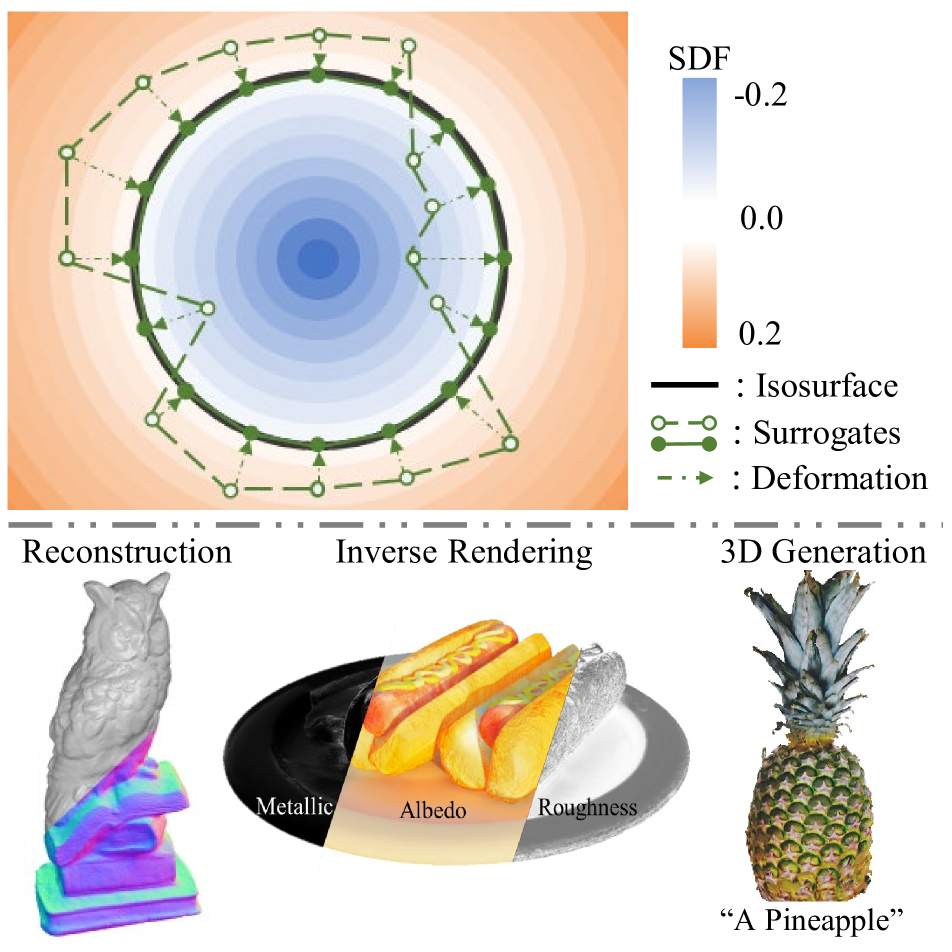
Figure 1: The proposed Sur²f and its applications.

1 Introduction

Surface reconstruction of 3D objects or scenes from a set of multi-view observed images is a classical and challenging problem in 3D vision research. The problem is ill-posed given that multi-view images are only 2D observations of the 3D contents. To achieve surface reconstruction, recent efforts [5, 49, 11, 51, 33, 52, 45] aim to build the inverse process of image projection or rendering, such that the underlying geometry and surface appearance can be recovered. The process involves modeling the underlying geometry and appearance for inverse rendering, for which different surface representations can be adopted. For example, one may represent the surface explicitly as a polygonal mesh and use an associated shading function for surface rendering; alternatively, one may model the surface geometry as (level set of) an implicit field (e.g., signed distance function (SDF) [34] or occupancy/opacity field [28, 29]), and render images of different views via volume rendering [29]. By parameterizing either explicit or implicit surface representations and developing differentiable versions of the corresponding surface or volume rendering techniques [24, 19, 29, 52, 45], the underlying surface can be recovered.

The explicit representation of a triangle mesh is compatible with the existing graphics pipeline, and it supports efficient rendering (e.g., via rasterization or ray casting); however, directly optimizing the mesh parameterization (e.g., positions of vertices, edge connections, etc.) in the context of inverse rendering is less convenient, since complex topologies are difficult to be obtained in the optimization process. In contrast, an implicit representation models the geometry by learning in the continuous 3D space, and consequently, it supports smooth optimization of model parameters and geometry of complex topologies can be recovered by isosurface extraction from the learned field function; however, learning via volume rendering of an implicit field is of low efficiency and less precise in terms of recovering the sharp surface [29]. Given these pros and cons of different representations, a few hybrid representations [39, 40] have been proposed aiming for better leveraging of their respective advantages. Notably, DMTet [39] proposes to learn a signed distance function that controls the deformation of a parameterized tetrahedron, and with a differentiable marching tetrahedra layer for mesh extraction, it supports efficient and differentiable surface rendering that enables learning from the observed multi-view images. DMTet is improved by FlexiCubes [40] and is used in NVDIFFREC [31] for jointly optimizing shape, material, and lighting from multi-view images. However, implicit functions used in DMTet and its variants are discretely defined on tetrahedral grid vertices, and as such, the key benefits of optimization in continuous 3D spaces from implicit field representations are only enjoyed partially; in addition, they do not support rendering from its implicit functions and thus cannot directly receive supervisions from the image observations.

In this work, we propose a new hybrid representation that aims to make a better use of the explicit and implicit surface representations. Technically, we learn two parallel streams of an implicit SDF and an explicit, surrogate surface (Sur²f) mesh; Fig.2 gives an illustration. We term our proposed representation as Sur²f, given that this surrogate plays an essential role in the learning. More specifically, we enforce learning of the pair of representations to be synchronized by driving the deformation of the surrogate mesh with functions induced from the implicit SDF. For the implicit stream, we use SDF-induced volume rendering [52, 45] to receive supervision from images of view observations. For the stream of explicit surrogate, we use efficient and differentiable surface rendering to receive additional supervision. We unify volume rendering and surface rendering of the two streams with a shared, neural shader, which is parameterized to support photorealistic rendering. Sharing the neural shader between the two representations is crucial to our proposed Sur²f, as it promotes the two parallelly learned representations to converge to the same surface. Maintaining the synchronized surrogate surface mesh also brings an important benefit for volume rendering — it improves the sampling efficiency per ray greatly, which consequently improves the quality of volume rendering. To verify our proposed Sur²f, we conduct thorough experiments in the contexts of inverse rendering and multi-view surface reconstruction. Experiments show that in terms of both recovery quality and recovery efficiency, our method is better than both the existing hybrid representations and the existing methods of multi-view surface reconstruction. As a general hybrid representation, we show the usefulness of Sur²f for other surface modeling and reconstruction tasks as well. We summarize our technical contributions as follows.

• We propose a new hybrid representation, termed Sur²f, that can enjoy the benefits of both explicit and implicit surface representations. This is achieved by learning two parallel streams of an implicit SDF and an explicit surrogate surface mesh, both of which, by rendering, receive supervision from multi-view image observations.

• We unify volume rendering of the implicit SDF and surface rendering of the surrogate mesh with a shared, neural shader, which promotes the two parallelly learned representations to converge to the same surface.

• Learning of the surrogate mesh is synchronized by driving its deformation with functions induced from the implicit SDF. The surrogate mesh also enables surface-guided volume sampling, which greatly improves the sampling efficiency per ray in volume rendering.

• We conduct thorough experiments in various task settings of surface reconstruction from multi-view images. Our proposed Sur²f outperforms existing surface representations and reconstruction methods in terms of both recovery quality and recovery efficiency.

2 Related Works

In this section, we briefly review the literature of explicit and implicit surface representations, and how they can be respectively rendered in a differentiable manner. We also review representative methods of hybrid representations. Some of these methods are state-of-the-art for the tasks of inverse rendering and multi-view surface reconstruction.

Differentiable rendering of explicit meshes Traditional graphics pipelines (e.g. OpenGL [41]) offer hardware-accelerated rendering capabilities, however, they incorporate a discretization phase of rasterizing polygonal meshes that prevents the rendering process from being differentiable. Recent efforts [24, 5, 19] develop differentiable versions of the rasterization and facilitate studies [11, 49, 43, 56] to infer 3D geometry from 2D images. Specifically, these studies optimize mesh vertices through gradient backpropagated from the rendering process, yet the optimization of complex topologies remains an unresolved problem.

Volume rendering of implicit fields Popular implicit representations include SDF [34], occupancy field [28], and density/opacity field [29]. For rendering, early surface rendering methods [32, 25, 51] seek ray intersection with the underlying surface represented by SDF or occupancy field and estimate shading color with a neural network. Recent volumetric rendering methods [29, 30, 4] marching rays through the whole space that are represented by density/opacity field for rendering. NeuS [45] and VolSDF [52] provide conversions from SDF into density for volume rendering. And their follow-up works [47, 22, 50, 20, 48, 10, 3, 9, 46] make efforts to improve the quality and/or efficiency. Notably, UNISURF [33] gradually reduces sampling region to encourage volume rendering to surface rendering.

Hybrid surface representations There also exist some hybrid surface representations in the literature. DMTet [39] and its subsequent work FlexiCubes [40] represent a surface with explicit grid and implicit SDF, where mesh could be extracted by differentiable marching operation. They are adopted by NVDIFFREC [31] for physically based inverse rendering from multi-view images.

3 Preliminaries on rendering of different surface representations

In this section, we present representatives of existing rendering techniques for either implicit or explicit surface representations, which also prepare for the presentation of our proposed, new hybrid representation.

Rendering of an implicit SDF An SDF-based implicit representation can be either volume-rendered [52, 45], following NeRF [29], or directly rendered on the surface [51]. For volume rendering of an SDF, we denote a ray emanating from the camera center and through the rendering pixel as $\bm{r}(t)=\bm{o}+t\bm{\omega}$, $t\geq 0$, where $\bm{o}\in\mathbb{R}^{3}$ is the camera center and $\bm{\omega}\in\mathbb{R}^{3}$, $\|\bm{\omega}\|=1$, denotes the unit vector of viewing direction. Assume $N$ points are sampled along $\bm{r}$ and we write the $i$-th sampled point as $\bm{x}_{i}=\bm{r}(t_{i})=\bm{o}+t_{i}\bm{\omega}$; the shading color accumulated along the ray $\bm{r}$ can be approximated using the quadrature rule [27] as:

$$\bm{C}_{v}(\bm{r})=\sum^{N}_{i=1}T_{i}\alpha_{i}\bm{c}_{v}(\bm{x}_{i},\bm{n}_{i},\bm{\omega}),$$ (1)

$$T_{i}=\prod^{i-1}_{j=1}(1-\alpha_{j}),\quad\alpha_{i}=1-\exp(-\tau(\bm{x}_{i})\delta_{i}),$$

where $\delta_{i}=t_{i+1}-t_{i}$ denotes the distance between adjacent samples. While NeRF uses an MLP to directly encode the volume density $\tau:\mathbb{R}^{3}\rightarrow\mathbb{R}_{+}$, VolSDF [52] and NeuS [45] further show that $\tau$ can be modeled as a transformed function of the implicit SDF $f:\mathbb{R}^{3}\rightarrow\mathbb{R}$ , enabling better recovery of the underlying geometry. An SDF can also be used for neural surface rendering. For example, in [51], the intersection of the ray and the surface represented by an SDF is obtained by the sphere tracing algorithm [13] and is then fed into a neural shader to estimate the shading color.

Rendering of an explicit surface An explicit surface mesh can be rendered with better consideration of physical properties, i.e., physics-based rendering (PBR). Denote a triangle mesh as $\mathcal{S}=\{\mathcal{V},\mathcal{F}\}$, which is composed of a set $\mathcal{V}$ of vertices $\{\bm{v}\in\mathbb{R}^{3}\}$ and a set $\mathcal{F}$ of faces. Assume that a ray $\bm{r}$ intersects $\mathcal{S}$ at the surface point $\bm{x}_{\mathcal{S}}=\bm{r}(t_{\mathcal{S}})$, and we denote the surface normal as $\bm{n}_{\bm{x}_{\mathcal{S}}}$. The shading for the surface point $\bm{x}_{\mathcal{S}}$ from a camera view $\bm{{\omega}}$ is formulated as the non-emissive rendering equation [15]:

$$L(\bm{x}_{\mathcal{S}},\bm{\omega})=\int_{\Omega}L_{i}(\bm{x}_{\mathcal{S}},\bm{l})B(\bm{l},-\bm{\omega})\left<\bm{l}\cdot\bm{n}_{\bm{x}_{\mathcal{S}}}\right>d\bm{l},$$ (2)

where $\Omega$ denotes the hemisphere centered at $\bm{x}_{\mathcal{S}}$ and rotating around $\bm{n}_{\bm{x}_{\mathcal{S}}}$, $\bm{l}\in\mathbb{R}^{3}$, $\|\bm{l}\|=1$, denotes an incoming light direction, $L_{i}(\bm{x},\bm{l})$ denotes the incoming radiance of $\bm{x}$ from $\bm{l}$, $\left<\cdot\right>$ is a descriptor that computes the cosine of two input vectors, and $B$ is the bidirectional reflectance distribution function (BRDF) that describes the portion of reflected radiance at direction $-\bm{\omega}$ from direction $\bm{l}$. Based on the basic rendering of Eq. 2, [51, 49] use MLP-based neural shaders to approximate PBR; more specifically, a coordinate-based MLP takes the intersection point $\bm{x}_{\mathcal{S}}$, its associated surface normal $\bm{n}_{\bm{x}_{\mathcal{S}}}$, and the view direction $\bm{\omega}$ as inputs, and learns to output the shading result as:

$$\bm{C}_{s}(\bm{r})=\bm{c}_{s}(\bm{x}_{\mathcal{S}},\bm{n}_{\bm{x}_{\mathcal{S}}},\bm{\omega}).$$ (3)

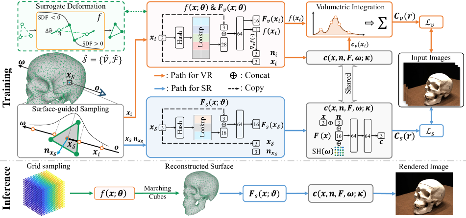
Figure 2: Overview of Sur²f. Sur²f learns parallel streams of an implicit SDF $f$ and a surrogate surface mesh $\widehat{\mathcal{S}}=\{\widehat{\mathcal{V}},\widehat{\mathcal{F}}\}$. Deformation of vertices $\{\widehat{\mathcal{V}}\}$ of the surrogate $\widehat{\mathcal{S}}$ is driven by functions induced from $f$, which enforces synchronization of the two representations (cf. Section 4.2). We use a shared, neural shader for both SDF-induced volume rendering and surface rendering of $\widehat{\mathcal{S}}$ (cf. Section 4.3), which enables dual supervisions from image observations. We also use surface-guided volume sampling (i.e., guided by $\widehat{\mathcal{S}}$) to improve the sampling efficiency (and consequently reconstruction quality) of volume rendering (cf. Section 4.4). During inference, we use marching cubes [26] to extract a mesh $\mathcal{S}$ from $f$; with the already learned neural shader, we achieve photorealisc, real-time rendering from Sur²f.

4 The proposed hybrid representation

We present our proposed hybrid representation in the context of surface reconstruction from multi-view image observations. Given a set of calibrated RGB images $\{\bm{I}_{m}\}^{M}_{m=1}$ of a 3D scene, the task is to reconstruct the scene surface $\mathcal{S}$ and the associated surface appearance. Under the framework of differentiable rendering, the task boils down as modeling and learning the appropriate surface representations that are rendered to match $\{\bm{I}_{m}\}^{M}_{m=1}$. As discussed in Sections 1 and 3, one may rely either on volume rendering of an implicit field, or on surface rendering of an explicit mesh; each of them has its own merits, while being limited in other aspects. Simply to say, volume rendering of implicit fields is easier to be optimized and has the flexibility in learning complex typologies; it is, however, of low efficiency and less compatibility with existing graphics pipelines. In contrast, surface rendering of explicit meshes has the opposite pros and cons. We are thus motivated to propose a new, hybrid representation that can benefit from both representations. We technically achieve the goal by learning a synchronized pair of an implicit SDF $f$ and an explicit surrogate surface (Sur²f) mesh $\widehat{\mathcal{S}}=\{\widehat{\mathcal{V}},\widehat{\mathcal{F}}\}$; we enforce their synchronization by driving the iterative deformation of $\widehat{\mathcal{S}}$ with functions induced from the implicit $f$ that is optimized to the current iteration. We further unify SDF-induced volume rendering of $f$ and surface rendering of $\widehat{\mathcal{S}}$ with a shared, neural shader, where the synchronized $\widehat{\mathcal{S}}$ is also used to greatly improve the sampling efficiency in volume rendering. Fig. 2 gives an illustration. Compared with the hybrid representation of DMTet [39], the implicit part of Sur²f is continuously defined and can be directly rendered to receive supervision from $\{\bm{I}_{m}\}^{M}_{m=1}$. Consequently, Sur²f is expected to be better in terms of surface modeling and reconstruction. In Section 5, we validate our proposed Sur²f for experiments of multi-view surface reconstruction as well as other surface modeling tasks.

4.1 SDF-induced volume rendering

As shown in the top, orange path in Fig. 2, we learn a neural implicit function of SDF $f(\cdot;\bm{\theta})\in\mathbb{R}$ whose zero-level set represents the underlying surface $\mathcal{S}=\{\bm{x}\in\mathbb{R}^{3}|f(\bm{x})=0\}$ to be reconstructed; $f(\cdot;\bm{\theta})$ takes any space point $\bm{x}\in\mathbb{R}^{3}$ as input and returns its signed distance to $\mathcal{S}$. In this work, we implement $f(\cdot;\bm{\theta})$ as an MLP and encode any $\bm{x}$ using multi-resolution hash grid [30], before feeding into the network. For any space point $\bm{x}$, except for the signed distance value $f(\cdot;\bm{\theta})$, we also learn its feature as $\bm{F}_{v}(\bm{x};\bm{\theta})$, using the same MLP network, as shown in Fig. 2; note that both $f(\cdot;\bm{\theta})$ and $\bm{F}_{v}(\bm{x};\bm{\theta})$ are parameterized by the same $\bm{\theta}$.

Given $f$, we conduct SDF-induced volume rendering, following NeuS [45], where the discrete opacity $\alpha_{i}$ in Eq. 1 is described as:

$$\alpha_{i}=\max\left(\frac{\Phi_{s}(f(\bm{x}_{i}))-\Phi_{s}(f(\bm{x}_{i+1}))}{\Phi_{s}(f(\bm{x}_{i}))},0\right),$$ (4)

where $\Phi_{s}(z)=1/(1+e^{-sz})$ is the Sigmoid function, $s$ is a learnable parameter, and $\bm{x}_{i}=\bm{r}(t_{i})=\bm{o}+t_{i}\bm{\omega}$ is a sampled point along a ray $\bm{r}$. We also note that a normal $\bm{n}_{i}$ at $\bm{x}_{i}$ can be computed as the derivation of $f$: $\bm{n}_{i}=\nabla_{\bm{x}_{i}}f(\bm{x}_{i})$.

4.2 Learning a synchronized surrogate of explicit mesh

A useful hybrid surface representation expects an explicit mesh whose deformation is synchronized with (zero-level set of) the implicit $f$. This can be simply achieved by applying isosurface extraction per iteration from the updated $f$, as in [39, 40]. However, isosurface extraction per iteration is computationally expensive, and more importantly, for a hybrid representation, it may not provide complementary benefits on the surface learning, since the extracted mesh is equivalent to the implicit field updated per iteration.

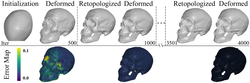
Figure 3: Visualization of the synchronized deformation of the surrogate mesh. Each error map shows the distance between the surrogate mesh and the mesh extracted from the SDF $f$ at a certain training iteration.

In this work, we propose to maintain an explicit, surrogate surface mesh $\widehat{\mathcal{S}}=\{\widehat{\mathcal{V}},\widehat{\mathcal{F}}\}$ at a much lower computational cost, whose iterative deformation is driven by, but not directly extracted from, $f$. More specifically, we deform each vertex $\hat{\bm{v}}\in\widehat{\mathcal{V}}$ per iteration according to:

$$\hat{\bm{v}}\leftarrow\hat{\bm{v}}-\eta\Delta\hat{\bm{v}},$$ (5)

$$\textrm{with}\quad\eta=f(\hat{\bm{v}}), \quad\Delta\hat{\bm{v}}=\nabla_{\hat{\bm{v}}}f(\hat{\bm{v}})/\left\|\nabla_{\hat{\bm{v}}}f(\hat{\bm{v}})\right\|_{2}.$$

An initial $\widehat{\mathcal{S}}$ can be obtained by applying marching cubes [26] to an SDF $f$ whose zero-level set is assumed to capture an initial surface (e.g., a sphere). We conduct empirical analysis on the synchronization via rule (Eq. 5) between $\widehat{\mathcal{S}}$ and $f$ (cf. Section 5 for details of the empirical setting). Fig. 3 shows that when the training of Sur²f proceeds, the difference between $\widehat{\mathcal{S}}$ and the zero-level set of $f$ is gradually reduced. Indeed, training improves the conditioning of the level sets of $f$, and in the ideal case, we have $\nabla_{\bm{x}_{i}}f(\bm{x}_{i})\sim\nabla_{\bm{x}_{j}}f(\bm{x}_{j})\sim\nabla_{\bm{x}_{0}}f(\bm{x}_{0})$ for any pair of $\bm{x}_{i}$ and $\bm{x}_{j}$ that are on different level sets of $f$, i.e., $f(\bm{x}_{i})\neq f(\bm{x}_{j})$, but correspond to the same surface point $\bm{x}_{0}$, where $f(\bm{x}_{0})=0$; in other words, normals at these space points are parallel. When coming to this ideal case, we have $f\big{(}\bm{x}-f(\bm{x})\nabla_{\bm{x}}f(\bm{x})/\left\|\nabla_{\bm{x}}f(\bm{x})\right\|_{2}\big{)}=0$, which means that a single-step updating by (Eq. 5) synchronizes the two representations. In practice, we observe approaching of this ideal case at later stages of training, at least for space points near the surface. Considering that the deformation (Eq. 5) itself is not guaranteed to meshes of complex topologies, we periodically apply marching cubes to re-boot the process; ablation study in Section 5 shows that re-booting every 500 iterations is enough to produce high-quality meshes while keeping a high efficiency.

4.3 Unifying surface rendering and volume rendering with a shared shading network

Given the surrogate surface $\widehat{\mathcal{S}}$, a surface point $\bm{x}_{\widehat{\mathcal{S}}}=\bm{r}(t_{\widehat{\mathcal{S}}})=\bm{o}+t_{\widehat{\mathcal{S}}}\bm{\omega}$ can be efficiently and exactly obtained in a device-native manner (e.g., via rasterization or ray casting), which is an intersection of the ray $\bm{r}$ and $\widehat{\mathcal{S}}$. For any $\bm{x}_{\widehat{\mathcal{S}}}$, we use an MLP, parameterized by $\bm{\vartheta}$, to learn its geometric feature as $\bm{F}_{s}(\bm{x}_{\widehat{\mathcal{S}}};\bm{\vartheta})$, and we again encode $\bm{x}_{\widehat{\mathcal{S}}}$ using multi-resolution hash grid [30], before feeding into the MLP network. The surface normal $\bm{n}_{\widehat{\mathcal{S}}}$ at $\bm{x}_{\widehat{\mathcal{S}}}$ is the normal vector associated with the intersecting triangle face [2]. The bottom, blue path in Fig. 2 gives the illustration.

Comparing the shading function $\bm{c}_{v}(\bm{x}_{i},\bm{n}_{i},\bm{\omega})$ in (Eq. 1) for volume rendering $\bm{C}_{v}(\bm{r})$ of a ray $\bm{r}$ and its counterpart $\bm{c}_{s}(\bm{x}_{\mathcal{S}},\bm{n}_{\mathcal{S}},\bm{\omega})$ in (Eq. 3) for surface rendering $\bm{C}_{s}(\bm{r})$ at the ray-surface intersection, one may be tempted to unify them using a same shading function. In fact, given appropriate hypothesis spaces of functions, both shading functions can model PBR [51]. The difference lies in that volume rendering of (Eq. 1) weights and sums the shadings for $\{\bm{x}_{i}\}$ sampled along $\bm{r}$, while surface rendering of (Eq. 3) concentrates sharply on the surface point; as such, the two ways of shading converge to an identical one when the distribution of weights in (Eq. 1) (i.e., $\{T_{i}\alpha_{i}\}$) approaches to a Dirac one. In this work, we propose surface-guided volume sampling (cf. Section 4.4) that practically enhances this effect. Also considering that an MLP of enough capacity is a universal function approximator, we propose to unify $\bm{c}_{v}(\bm{x}_{i},\bm{n}_{i},\bm{\omega})$ and $\bm{c}_{s}(\bm{x}_{\mathcal{S}},\bm{n}_{\mathcal{S}},\bm{\omega})$ using a shared neural shader $\bm{c}(\bm{x},\bm{n},\bm{F},\bm{\omega};\bm{\kappa})$, parameterized by $\bm{\kappa}$, where we also augment with a feature $\bm{F}$ that encodes the local geometry around $\bm{x}$. $\bm{c}(\bm{x},\bm{n},\bm{F},\bm{\omega};\bm{\kappa})$ is instantiated as $\bm{c}(\bm{x}_{i},\bm{n}_{i},\bm{F}_{v}(\bm{x}_{i}),\bm{\omega};\bm{\kappa})$ for volume rendering of sampled $\{\bm{x}_{i}\}$ along a ray, and as $\bm{c}(\bm{x}_{\widehat{\mathcal{S}}},\bm{n}_{\bm{x}_{\widehat{\mathcal{S}}}},\bm{F}_{s}(\bm{x}_{\widehat{\mathcal{S}}}),\bm{\omega};\bm{\kappa})$ for rendering of a surface point on the surrogate $\widehat{\mathcal{S}}$. In practice, we also use sphere harmonics [53] to encode the view direction, denote as $\texttt{SH}(\bm{\omega})$, before feeding into the neural shader.

4.4 Improving the efficiency and quality via surface-guided volume sampling

Volume rendering generates high-quality colors with no requirement of precise surface recovery [29], but at the cost of dense point sampling along rays. Previous methods either uniformly sample points along a ray [30, 47, 21], or employ hierarchical sampling [29] that obtains points close to the surface in a multi-step fashion [45, 52]; both strategies involve heavy computations and result in slow convergence.

With a maintained and synchronized surrogate $\widehat{\mathcal{S}}$ in Sur²f, we expect it could be useful for guiding the point sampling in volume rendering, since for any ray $\bm{r}$, the ray-surface intersection can be efficiently and exactly obtained via rasterization or ray casting. Let $\bm{x}_{\widehat{\mathcal{S}}}=\bm{r}(t_{\widehat{\mathcal{S}}})$ be the intersection point, we conduct point sampling along $\bm{r}$ as

$$\bm{x}_{i}=\bm{r}(t_{i})=\bm{o}+t_{i}\bm{\omega}\quad\textrm{s.t.}\quad t_{i}\sim\mathcal{N}(t_{\widehat{\mathcal{S}}},\sigma^{2}),$$ (6)

where $\sigma^{2}$ is the variance that controls the tightness of the sampled points around $\bm{x}_{\widehat{\mathcal{S}}}$. We anneal $\sigma$ linearly w.r.t. the optimization iteration, such that the sampled points are distributed around the surface gradually. For each of those rays that do not intersect $\widehat{\mathcal{S}}$, we simply use uniform sampling along the ray. Volume sampling guided by $\widehat{\mathcal{S}}$ improves the efficiency greatly, as verified in Section 5. It also improves the quality of volume rendering, since the learning is much concentrated on the surface. Empirical results in Section 5 corroborate our analysis.

4.5 Training and Inference

To train Sur²f, in each iteration, we randomly sample pixels from the observed images and define the set of camera rays passing through these pixels as $\mathcal{R}$. By compactly writing $\bm{C}_{v}(\bm{r};\bm{\theta},\bm{\kappa})=\sum_{i=1}^{N}T_{i}\alpha_{i}\bm{c}(\bm{x}_{i},\bm{n}_{i},\bm{F}_{v}(\bm{x}_{i};\bm{\theta}),\bm{\omega};\bm{\kappa})$ and $\bm{C}_{s}(\bm{r};\bm{\vartheta},\bm{\kappa})=\bm{c}(\bm{x}_{\widehat{\mathcal{S}}},\bm{n}_{\bm{x}_{\widehat{\mathcal{S}}}},\bm{F}_{s}(\bm{x}_{\widehat{\mathcal{S}}};\bm{\vartheta}),\bm{\omega};\bm{\kappa})$, we train Sur²f by minimizing the following loss:

$$\mathcal{L}_{s} =\frac{1}{|\mathcal{R}|}\sum_{\bm{r}\in\mathcal{R}}\texttt{L1}\left(\bm{C(r)},\bm{C}_{s}(\bm{r};\bm{\vartheta},\bm{\kappa})\right),$$ (7)

$$\mathcal{L}_{v} =\frac{1}{|\mathcal{R}|}\sum_{\bm{r}\in\mathcal{R}}\texttt{Smooth}_{\texttt{L1}}\left(\bm{C(r)},\bm{C}_{v}(\bm{r};\bm{\theta},\bm{\kappa})\right),$$

$$\mathcal{L} =\lambda_{s}\mathcal{L}_{s}+\lambda_{v}\mathcal{L}_{v}+\mathcal{L}_{\text{\tiny Eik}},$$

where $\bm{C(r)}$ is the observed color for ray $\bm{r}$, and $\mathcal{L}_{\text{\tiny Eik}}$ is the Eikonal loss [12] that regularizes the learning of SDF $f$. $\lambda_{s}$ and $\lambda_{v}$ are hyperparameters weighting different loss terms. In addition, we optimize an optional binary cross-entropy (BCE) loss once the image masks are available:

$$\mathcal{L}_{\text{\tiny mask}}=\frac{1}{|\mathcal{R}|}\sum_{\bm{r}\in\mathcal{R}}\mathds{1}_{\text{\tiny mask}}(\bm{r})\texttt{BCE}\left(m(\bm{r}),O(\bm{r})\right),$$ (8)

where $\mathds{1}_{\text{\tiny mask}}(\bm{r})$ indices whether the mask $m(\bm{r})$ of the ray is available, and $O(\bm{r})=\sum^{N}_{i=1}T_{i}\alpha_{i}$ is the opacity of ray $\bm{r}$. The mask loss is weighted by the hyperparameter $\lambda_{\text{\tiny mask}}$.

During inference, we use marching cubes [26] to extract a surface mesh $\mathcal{S}$ from the learned $f$. Given the simultaneously learned neural shader, we are able to conduct real-time, interactive rendering of $\mathcal{S}$ with the mesh rasterized by an off-the-shelf graphics pipeline.

5 Experiments

In this section, we first verify our proposed Sur²f in the context of surface reconstruction from multi-view images (cf. Section 4) on the DTU object benchmark dataset [14] by comparing with baselines (cf. Section 5.1) and designing elaborate experiments (cf. Section 5.2). Then we conduct comparisons with other hybrid representation methods (cf. Section 5.3) in the task of physically based inverse rendering from multi-view images on the NeRF synthetic dataset [29]. We further examine the applicability of Sur²f by applying it to the task of indoor and outdoor scene reconstruction (cf. Section 5.4) on ScanNet [8] and Tanks and Temples [18] datasets. We also apply Sur²f to text-to-3D generation (as in Fig. 1). More results are provided in the appendix.

Reference

NDS [49]

UNISURF [33]

NeuS [45]

NeuS2 [47]

Ours

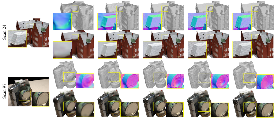
Figure 4: Qualitative comparisons on the DTU dataset [14]. The surface details are zoomed in and visualized as colors coded by surface normals for a better view. For each scene, the upper row is for geometry reconstruction while the lower row is for image synthesis.

	Scan	24	37	40	55	63	65	69	83	97	105	106	110	114	118	122	Mean	Time
CD $\downarrow$	NDS [49]	4.24	5.25	1.30	0.53	2.47	1.22	1.35	1.59	2.77	1.15	1.02	3.18	0.62	1.65	0.91	1.95	7min
	UNISURF [33]	1.32	1.36	1.72	0.44	1.35	0.79	0.80	1.49	1.37	0.89	0.59	1.47	0.46	0.59	0.62	1.02	22h
	NeuS [45]	0.83	0.98	0.56	0.37	1.13	0.59	0.60	1.45	0.95	0.78	0.52	1.43	0.36	0.45	0.45	0.77	6.5h
	NeuS2 [47]	0.56	0.76	0.49	0.37	0.92	0.71	0.76	1.22	1.08	0.63	0.59	0.89	0.40	0.48	0.55	0.70	5min
	Ours	0.50	0.67	0.44	0.35	0.89	0.62	0.71	1.18	1.06	0.75	0.59	0.78	0.38	0.49	0.44	0.66	5min
	Scan	24	37	40	55	63	65	69	83	97	105	106	110	114	118	122	Mean	RT
PSNR $\uparrow$	NDS [49]	20.03	21.30	25.16	24.69	26.69	26.84	24.20	30.19	24.15	28.04	25.73	25.82	26.65	18.08	31.49	25.27	5ms
	UNISURF [33]	26.98	25.34	27.30	27.62	32.76	32.77	29.85	34.15	28.84	32.50	33.47	31.45	29.60	35.49	35.76	30.93	>1min
	NeuS [45]	26.62	23.64	26.43	25.59	30.61	32.83	29.24	33.71	26.85	31.97	32.18	28.92	28.41	35.00	34.81	29.79	30s
	NeuS2 [47]	30.23	27.29	30.20	33.27	34.53	33.29	30.45	37.73	30.29	34.26	36.92	34.39	33.50	39.73	40.30	33.29	1s
	Ours	30.34	27.98	31.02	33.76	35.38	35.41	30.47	39.29	30.72	36.16	37.40	34.87	32.74	39.82	40.53	33.95	5ms

Table 1: Quantitative comparisons on the DTU dataset [14]. We compare the reconstructed geometry with baseline methods using Chamfer Distance. Our method achieves the best overall performance while performing as efficiently as NeuS2 [47] and much faster than other methods. For rendering PSNR comparisons, our method outperforms other methods in most cases for image synthesis quality with fast Rendering Time (RT). We mark the Best result and the Second best result.

Implementation Details We implement Sur²f in PyTorch[36] framework with CUDA extensions. We set the multi-resolution hash grids with 8 levels for the surface rendering branch and 14 levels for the volume rendering branch, where both hash resolutions range from 16 to 1024 with a feature dimension of 2, and set the spherical harmonics to 4 degree. During training, we employ the Adam optimizer [17] with a learning rate of 2e-3, and set the hyperparameters $\lambda_{s}$, $\lambda_{v}$, $\lambda_{\text{\tiny Eik}}$, and $\lambda_{\text{\tiny mask}}$ to 1, 1, 0.05, and 0.1, respectively. In each iteration, we sample a batch of 14800 rays, do ray casting with NVIDIA OptiX [35] engine, and use customized CUDA kernels to calculate the $\alpha$-compositing colors of the sampled points along each ray as Eq. 1. All experiments are conducted on a single GeForce RTX 3090 GPU. Further implementation details for different tasks can be found in the appendix.

Evaluation Metrics For surface reconstruction, we measure the recovered surfaces with Chamfer Distance (CD) [14]. To evaluate the image rendering qualities, we compute the peak signal-to-noise ratio (PSNR) between the reference images and the synthesized images. We compute the mean angle error (Mean-A) for the evaluation of normal maps.

5.1 Comparisons on DTU in the context of multi-view surface reconstruction

We evaluate both the geometry reconstruction metric and the rendering quality of our proposed Sur²f. We set NDS [49], NeuS [45], UNISURF [33], and NeuS2 [47] as our baselines. As NDS [49] optimizes explicit mesh with a differentiable surface rendering paradigm, NeuS [45] takes the SDF-induced volume rendering paradigm that we based on, UNISURF [33] proposes to unify these two rendering paradigms, and NeuS2 [47] serves as the speed baseline. The results are presented in Tab. 1. In the realm of geometry reconstruction, Sur²f achieves the best overall performance while maintaining the fastest convergence speed. The qualitative results showcased in Fig. 4 further illustrate Sur²f’s ability to swiftly capture fine-grained geometry details. Sur²f also demonstrates superior image synthesis quality and achieves fast rendering in mere milliseconds.

5.2 Ablation Studies

We design elaborate experiments to evaluate the designs of Sur²f that are stated in Section 4. These studies are conducted on the DTU dataset [14].

Analysis on the synchronization of Surface Surrogate Sur²f maintains an explicit, surrogate surface mesh, which is synchronized by driving the deformation induced from the implicit SDF $f$ (cf. Section 4.2). We visualize the surrogate deformation results and the distance between the surrogate mesh and the underlying surface represented by $f$ at certain training iterations in Fig. 3, which shows that the surrogate mesh is synchronized with the learning of $f$ and they together converge to the same surface. We also examine the intervals of iteration for applying isosurface extraction to re-boot the synchronization and various algorithms to perform the rebooting. As can be seen in Tab. 2, we find that an interval of 500 iterations strikes a balance between accuracy and efficiency, and Sur²f is not sensitive to the choice of isosurface extraction algorithms.

Analysis on the shared shading network We unify surface rendering and volume rendering with a shared shading network (cf. Section 4.3), which promotes the parallelly learned surrogate mesh and implicit SDF to converge to the same surface, as evidenced by the previous ablation. We further show the image synthesis results of the two rendering streams with/without learning a shared shader in Fig. 5. We observe significant discrepancies in renderings without a shared shader, which suggests a disruption in the synchronization between the surrogate mesh and the implicit SDF.

Analysis on the surface-guided volume sampling strategy With a maintained and synchronized surface surrogate, Sur²f further introduces a surface-guided volume sampling strategy to improve the sampling efficiency (cf. Section 4.4). We compare this ray sampling strategy with alternative approaches, including uniform sampling proposed by Nerfacc [21] and hierarchical sampling adopted by NeuS [45]. The results in Tab. 3 show that our surface-guided sampling strategy leads to more accurate reconstruction and higher quality of rendering while saving training time.

Algorithm Interval/iter	MC 1	MC 300	MC* 500	MC 700	MC 1000	DMTet 500	FlexiCubes 500
CD $\downarrow$	0.654	0.659	0.661	0.682	0.715	0.662	0.661
Time/s $\downarrow$	21869	384	348	335	324	358	359

Table 2: Analysis on different intervals of iteration and different isosurface extraction algorithms (i.e. Marching Cube (MC) [26], DMTet [39] and FlexiCubes [40]) for the retopology of surrogate.

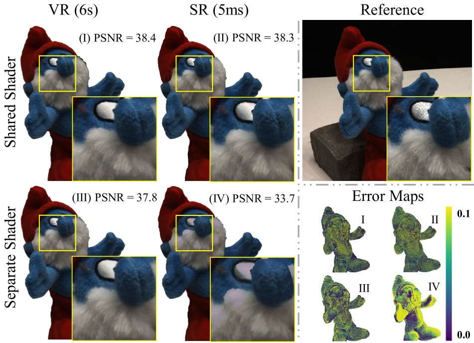
Figure 5: Visualization of images synthesized by Volume Rendering (VR) and Surface Rendering (SR) with/without learning a shared shading network. The error maps measure the absolute pixel distance between rendered images and reference.

	Surface-guided*	Uniform	Hierarchical
CD $\downarrow$	0.661	0.732	0.662
PSNR $\uparrow$	33.95	30.09	33.68
Time/s $\downarrow$	348	337	9538

Table 3: Analysis of ray sampling strategies for volume rendering.

Applications

Ours (0.4h)

FlexiCubes [40] (1.8h)

DMTet [39] (1.3h)

Reference (Time $\downarrow$)

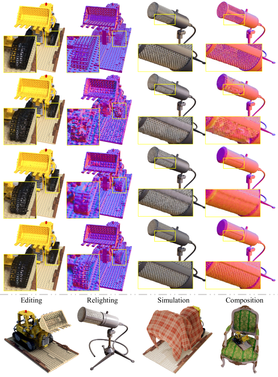
Figure 6: Qualitative results on the NeRF synthetic dataset [29]. The last row shows some applications with a 3D content creation tool Blender [6].

5.3 Comparison with other hybrid representations methods

We compare our proposed Sur²f with existing hybrid representations, i.e. DMTet [39] and FlexiCubes [40]. Notably, these representations find application in NVDIFFREC [31] for the task of physically based inverse rendering from multi-view images. Thus we extend Sur²f to the same task by incorporating the differentiable renderer from NVDIFFREC [31], and give the technical details in the appendix. We compare the recovered normal maps and rendering results with these hybrid representations and report the quantitative and qualitative results in Fig. 6 and Tab. 4, which demonstrate that Sur²f promotes better quality and efficiency and also enables many downstream applications with an existing 3D content creation tool Blender [6].

PSNR $\uparrow$	Chair	Drums	Ficus	Hotdog	Lego	Mats	Mic	Ship
DMTet	31.8	24.6	30.9	33.2	29.0	27.0	30.7	26.0
FlexiCubes	31.8	24.7	30.9	33.4	28.8	26.7	30.8	25.9
Ours	31.9	25.2	31.4	33.9	30.3	27.0	31.3	27.1
Mean-A $\downarrow$	Chair	Drums	Ficus	Hotdog	Lego	Mats	Mic	Ship
DMTet	22.1	27.8	28.6	14.6	40.5	13.9	21.0	34.2
FlexiCubes	16.6	22.3	25.2	9.3	32.9	14.3	19.4	39.7
Ours	14.0	20.0	22.1	8.6	29.2	12.0	16.3	22.7

Table 4: Quantitative results on the NeRF synthetic dataset [29].

5.4 Indoor and outdoor scene reconstruction

Reference

Helixsurf [23]

MonoSDF [54]

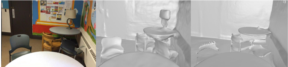
GT

Helixsurf with Sur2f

MonoSDF with Sur2f

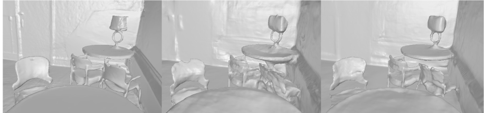
Figure 7: Qualitative results on ScanNet [8]. With Sur²f, details (e.g. the lamp, the chair back on the left) in the scene can be better reconstructed.

Reference (Time $\downarrow$)

Neuralangelo [22] (52h)

Ours (1h)

Figure 8: Qualitative results on Tanks and Temples [18]. Sur²f strikes a better quality-efficiency trade-off than Neuralangelo does.

As a general hybrid representation, Sur²f is also useful for indoor and large-scale outdoor reconstruction tasks. We incorporate Sur²f with existing indoor scene reconstruction methods, i.e. Helixsurf [23] and MonoSDF [54], to reconstruct the complex indoor scene from ScanNet [8]. And we reconstruct outdoor scenes from Tanks and Temples [18] by incorporating with Neuralangelo [22]. The results in Fig. 7 and Fig. 8 show that Sur²f enhances the recovery of intricate scene details and gains a better quality-efficiency trade-off.

6 Conclusion

In this paper, we introduce a new hybrid representation, named Sur²f. By learning two parallel streams of an implicit SDF and an explicit surrogate surface mesh, and unifying volume rendering and surface rendering with a shared neural shader, Sur²f exhibits outstanding performance across various surface modeling and reconstruction tasks. Our approach reaffirms the efficacy of combining traditional rendering techniques with contemporary, differentiable rendering-based neural learning for robust surface modeling and 3D representation.

Appendix

1 Additional details for multi-view surface reconstruction

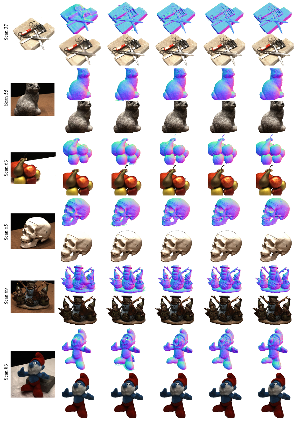
Figure 14: More qualitative results on the DTU dataset [14].

We use the same 15 object-centric scenes as in IDR [51] for quantitative and qualitative comparisons and analyses, where each scene provides 49 or 64 images with the resolution of 1600 $\times$ 1200 captured by a robot-held monocular RGB camera and ground truth point cloud obtained from a structured-lighted scanner. And the foreground masks are provided by IDR [51]. More qualitative results are shown in Fig. 14 and Fig. 15.

Reference

w/ mask

w/o mask

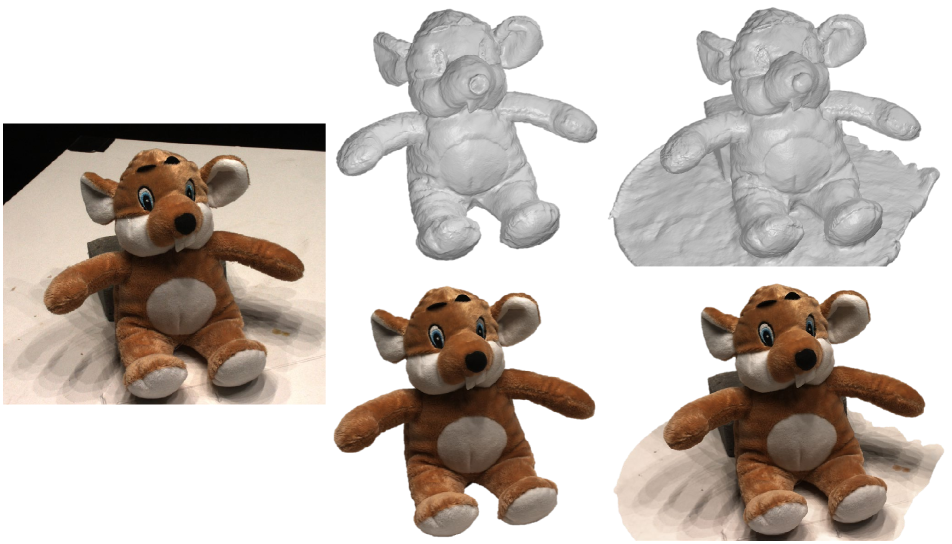
Figure 9: Visualization of example reconstructions with (w/) and without (w/o) foreground mask.

Sur²f also offers the flexibility to perform reconstruction without foreground masks. If the foreground masks are not available, we model the foreground and background using two separate models by spatially separating the representations. The foreground area of interest for Sur²f to reconstruct is defined as a sphere encompassing objects centered around an approximate scene center. Everything located outside the sphere is considered as background, which is represented with a NeRF model from NeRF++ [55]. Indeed, analogous strategies are adopted by NeuS [45] and Neuralangelo [22]. We provide visual results of reconstructions for these two settings in Fig. 9, which demonstrates that there is no noticeable difference in the reconstructions of the same foreground object. Furthermore, we find the evaluation metric of Chamfer Distance (w/ : 0.66 vs. w/o : 0.64) is close in these two settings as the evaluation is confined to the masked areas.

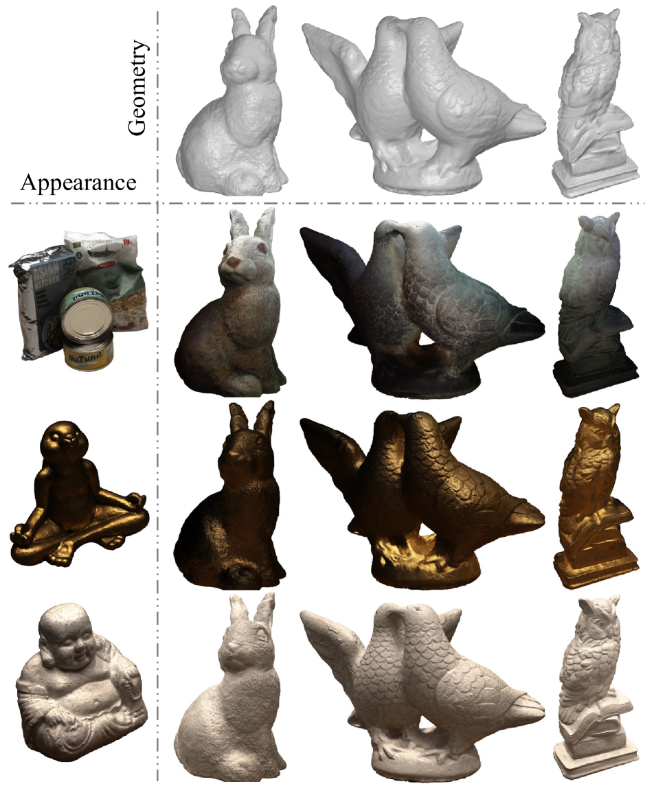
Figure 10: Transferring different appearances to different geometries.

The framework design (illustrated in Fig. 2) of Sur²f also facilitates the disentanglement between geometry and appearance [51]. Leveraging this separation of geometry and appearance, different appearances can be seamlessly transferred to different geometries by exchanging the shading network (cf. Section 4.3), as exemplified in Fig. 10.

2 Additional details for inverse rendering

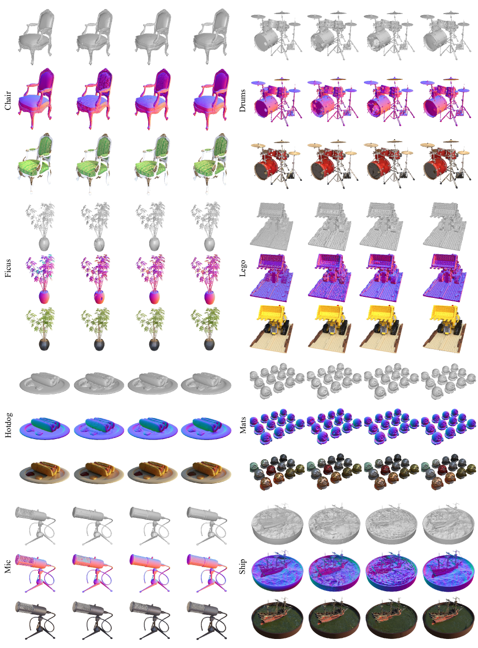
Figure 16: More qualitative results on the NeRF synthetic dataset [29].

In Section 5.3, we compare Sur²f with other hybrid representations in the task of physically based inverse rendering (PBR). To achieve the inverse rendering from multi-view images, we incorporate Sur²f with the differentiable render from NVDIFFREC [31]. We give the details here and report more qualitative results in Fig. 16.

Starting from the non-emissive rendering equation Eq. 2, we use the Lambertian diffuse model [1] and the Cook-Torrance microfacet specular model [7] to formulate the BRDF $B(\bm{l},-\bm{\omega})$:

$$B(\bm{l},-\bm{\omega})=\underbrace{(1-k_{m})\frac{\bm{k}_{d}}{\pi}}_{\text{diffuse}}+\underbrace{\frac{DFG}{4\left<\bm{n}\cdot\bm{l}\right>\left<\bm{n}\cdot-\bm{\omega}\right>}}_{\text{specular}},$$ (9)

where $\bm{k}_{d}\in[0,1]^{3}$ and $k_{m}\in[0,1]$ denote the base color and metallic value of surface point $\bm{x}_{\widehat{\mathcal{S}}}$ for the view-independent diffuse term. And for the view-dependent specular term, we define the surface roughness $k_{r}\in[0,1]$ to condition the microfacet distribution function ($D$), Fresnel reflection ($F$), and geometric shadowing factor ($G$). We obtain $\bm{k}_{d}$ and $\bm{k}_{rm}=(k_{r},k_{m})$ by adapting the surface geometric feature learning module $\bm{F}_{s}(\bm{x}_{\widehat{\mathcal{S}}};\bm{\vartheta})$, which is illustrated in Fig. 11.

According to Eq. 9, the rendering equation is:

$$L(\bm{x}_{\mathcal{S}},\bm{\omega})= \int_{\Omega}L_{i}(\bm{x}_{\mathcal{S}},\bm{l})B(\bm{l},-\bm{\omega})\left<\bm{l}\cdot\bm{n}_{\bm{x}_{\mathcal{S}}}\right>d\bm{l}$$ (10)

$$= \int_{\Omega}L_{i}(\bm{x}_{\mathcal{S}},\bm{l})\left[(1-k_{m})\frac{\bm{k}_{d}}{\pi}+\frac{DFG}{4\left<\bm{n}\cdot\bm{l}\right>\left<\bm{n}\cdot-\bm{\omega}\right>}\right]\left<\bm{l}\cdot\bm{n}_{\bm{x}_{\mathcal{S}}}\right>d\bm{l}$$

$$= (1-k_{m})\frac{\bm{k}_{d}}{\pi}\int_{\Omega}L_{i}(\bm{x}_{\mathcal{S}},\bm{l})\left<\bm{l}\cdot\bm{n}_{\bm{x}_{\mathcal{S}}}\right>d\bm{l}+$$

$$\int_{\Omega}L_{i}(\bm{x}_{\mathcal{S}},\bm{l})\frac{DFG}{4\left<\bm{n}\cdot\bm{l}\right>\left<\bm{n}\cdot-\bm{\omega}\right>}\left<\bm{l}\cdot\bm{n}_{\bm{x}_{\mathcal{S}}}\right>d\bm{l}$$

$$= L_{\text{diffuse}}(\bm{x}_{\mathcal{S}})+L_{\text{specular}}(\bm{x}_{\mathcal{S}},\bm{\omega}).$$

In this work, we follow NVDIFFREC [31] to use image-based lighting (IBL) to model the incident illumination, and employ split-sum approximation [16] to tackle the intractable integral. Thus the incident illumination can be represented as a learnable environment map $\bm{E}$, and the diffuse component $L_{\text{diffuse}}(\bm{x}_{\mathcal{S}})$ is defined as:

$$L_{\text{diffuse}}(\bm{x}_{\mathcal{S}})= (1-k_{m})\frac{\bm{k}_{d}}{\pi}\int_{\Omega}L_{i}(\bm{x}_{\mathcal{S}},\bm{l})\left<\bm{l}\cdot\bm{n}_{\bm{x}_{\mathcal{S}}}\right>d\bm{l}$$ (11)

$$\approx (1-k_{m})\frac{\bm{k}_{d}}{\pi}\ \bm{I}_{\text{d}},$$

where $\bm{I}_{\text{d}}$ denotes the diffuse irradiance obtained by integrating the upper hemisphere of the environment map $\bm{E}$. And for the specular component $L_{\text{specular}}(\bm{x}_{\mathcal{S}},\bm{\omega})$, we split the tricky integration into two trivial integrations and calculate these two integrals in advance:

$$L_{\text{specular}}(\bm{x}_{\mathcal{S}},\bm{\omega})=\int_{\Omega}L_{i}(\bm{x}_{\mathcal{S}},\bm{l})\frac{DFG}{4\left<\bm{n}\cdot\bm{l}\right>\left<\bm{n}\cdot-\bm{\omega}\right>}\left<\bm{l}\cdot\bm{n}_{\bm{x}_{\mathcal{S}}}\right>d\bm{l}$$ (12)

$$\approx \underbrace{\int_{\Omega}\frac{DFG}{4\left<\bm{n}\cdot\bm{l}\right>\left<\bm{n}\cdot-\bm{\omega}\right>}\left<\bm{l}\cdot\bm{n}_{\bm{x}_{\mathcal{S}}}\right>d\bm{l}}_{\text{Environment BRDF}-\bm{K}}\underbrace{\int_{\Omega}DL_{i}(\bm{x}_{\mathcal{S}},\bm{l})\left<\bm{l}\cdot\bm{n}_{\bm{x}_{\mathcal{S}}}\right>d\bm{l}}_{\text{Pre-Filtered Environment Map}-\bm{I}_{\text{s}}},$$

where $\bm{K}$ can be calculated in advance and stored in a 2D look-up texture, which can be search by roughness $k_{r}$ and $\left<\bm{n}\cdot-\bm{\omega}\right>$. And we convolve the environment map $\bm{E}$ with multi-level GGX distribution [44] to get the remaining $\bm{I}_{\text{s}}$. In summary, the approximated rendering equation is:

$$L(\bm{x}_{\mathcal{S}},\bm{\omega})\approx(1-k_{m})\frac{\bm{k}_{d}}{\pi}\ \bm{I}_{\text{d}}+\bm{K}\bm{I}_{\text{s}}.$$ (13)

Specifically, we integrate $\bm{I}_{\text{d}}$ and $\bm{I}_{\text{s}}$ from environment map $\bm{E}$ at the beginning of each training step, and get the rendered image color with standard linear-to-sRGB tone mapping [42]:

$$\bm{C}_{\text{pbr}}(\bm{r})=\texttt{ToneMap}(L(\bm{x}_{\mathcal{S}},\bm{\omega})).$$ (14)

The whole integration is differentiable to enable the additional loss optimization for PBR:

$$\mathcal{L}_{\text{pbr}}=\frac{1}{|\mathcal{R}|}\sum_{\bm{r}\in\mathcal{R}}\texttt{L1}\left(\bm{C(r)},\bm{C}_{\text{pbr}}(\bm{r})\right).$$ (15)

After optimization, we get the environment map $\bm{E}$ and the surface materials (i.e. albedo $\bm{k}_{d}$, roughness $k_{r}$, and metallic value $k_{m}$) suitable for the downstream applications (e.g. editing and relighting), and we show some examples in Fig. 12.

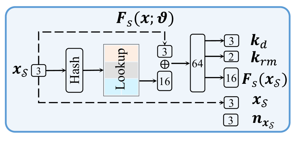
Figure 11: Adapted module for physically based inverse rendering.

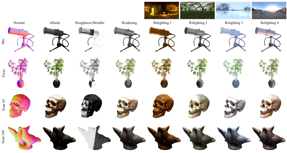
Figure 12: Reconstruction results and relighting application of physically based inverse rendering. The objects of the first two rows are from the NeRF synthetic dataset [29], and the last two rows are from the DTU dataset [14].

3 Additional details for indoor scene reconstruction

For indoor scene reconstruction (cf. Section 5.4), we incorporate the method with iterative intertwined regularization (i.e. Helixsurf [23]) and the method with monocular geometric cues (i.e. MonoSDF [54]) to address the challenge of rich textureless areas within the complex indoor scene. Both of the methods rely on the supervision of depths and normals, hence, we derive Sur²f to get the depth and normal for each ray $\bm{r}$ from Eq. 1 as:

$$d(\bm{r})=\sum^{N}_{i=1}T_{i}\alpha_{i}t_{i},\quad\bm{n}(\bm{r})=\sum^{N}_{i=1}T_{i}\alpha_{i}\bm{n}_{i}.$$ (16)

With the proposed surrogate surface, we check the multi-view geometric consistency and give the losses as:

$$\mathcal{L}_{\text{\tiny depth}}=\frac{1}{|\mathcal{R}|}\sum_{\bm{r}\in\mathcal{R}}\Gamma\left(0.05,\left\|\widetilde{d(\bm{r})}-t_{\widehat{\mathcal{S}}}\right\|_{1}\right)\texttt{L1}\left(\widetilde{d(\bm{r})},d(\bm{r})\right),$$ (17)

$$\mathcal{L}\text{\tiny normal}=\frac{1}{|\mathcal{R}|}\sum_{\bm{r}\in\mathcal{R}}\Gamma\left(\left<\widetilde{\bm{n}(\bm{r})}\cdot\bm{n}_{\bm{x}_{\widehat{\mathcal{S}}}}\right>,0.5\right)\texttt{L1}\left(\widetilde{\bm{n}(\bm{r})},\bm{n}(\bm{r})\right),$$

$$\Gamma(x,y)=\left\{\begin{array}[]{l}1\quad\text{if }x\geq y\\ 0\quad\text{if }x<y,\end{array}\right.$$

where $\widetilde{d(\bm{r})}$ and $\widetilde{\bm{n}(\bm{r})}$ are the depth and normal supervision provided by Helixsurf [23] or MonoSDF [54], $\left<\cdot\right>$ is a descriptor that computes the cosine of two input vectors, $t_{\widehat{\mathcal{S}}}$ is given near Eq. 6.

4 Additional details for text-to-3D generation

For text-to-3D generation, we use the latent space diffusion model of Stable Diffusion [38] as our guidance. To update the parameters $\bm{\theta},\bm{\vartheta},\bm{\kappa}$ in Sur²f, we calculate the gradient by the Score Distillation Sampling (SDS) losses [37]:

$$\nabla_{(\bm{\theta},\bm{\kappa})} \mathcal{L}_{\text{\tiny SDS}}(\phi,\bm{\mathsf{x}}=\{\bm{C}_{v}(\bm{r};\bm{\theta},\bm{\kappa})\})$$ (18)

$$=\mathbb{E}\left[\textit{\text{w}}(\mathsf{t})\left(\hat{\epsilon}_{\phi}(\bm{\mathsf{z}}_{\mathsf{t}}^{\bm{\mathsf{x}}};\mathsf{y},\mathsf{t})-\epsilon\right)\frac{\partial\bm{\mathsf{x}}}{\partial(\bm{\theta},\bm{\kappa})}\frac{\partial\bm{\mathsf{z}}^{\bm{\mathsf{x}}}}{\partial\bm{\mathsf{x}}}\right],$$

$$\nabla_{(\bm{\vartheta},\bm{\kappa})} \mathcal{L}_{\text{\tiny SDS}}(\phi,\bm{\mathsf{x}}=\{\bm{C}_{s}(\bm{r};\bm{\vartheta},\bm{\kappa})\})$$

$$=\mathbb{E}\left[\textit{\text{w}}(\mathsf{t})\left(\hat{\epsilon}_{\phi}(\bm{\mathsf{z}}_{\mathsf{t}}^{\bm{\mathsf{x}}};\mathsf{y},\mathsf{t})-\epsilon\right)\frac{\partial\bm{\mathsf{x}}}{\partial(\bm{\vartheta},\bm{\kappa})}\frac{\partial\bm{\mathsf{z}}^{\bm{\mathsf{x}}}}{\partial\bm{\mathsf{x}}}\right],$$

where the rendered image $\bm{\mathsf{x}}$ connects with the image encoder of the pre-trained stable diffusion model that is parameterized as $\phi$, $\bm{\mathsf{z}}^{\bm{\mathsf{x}}}$ is the encoded latent code, $\hat{\epsilon}_{\phi}(\bm{\mathsf{z}}_{\mathsf{t}}^{\bm{\mathsf{x}}};\mathsf{y},\mathsf{t})$ is the predicted noise given text embedding $\mathsf{y}$ and timestep $\mathsf{t}$, and $\epsilon$ is the noise added in $\bm{\mathsf{z}}^{\bm{\mathsf{x}}}$; and $\textit{\text{w}}(\mathsf{t})$ is a weighting function. We give some generated examples in Fig. 13.

A blue tulip

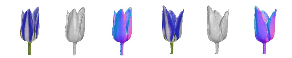
A delicious croissant

A pineapple

Figure 13: Examples of Text-to-3D Generation.

Reference

NDS [49]

UNISURF [33]

NeuS [45]

NeuS2 [47]

Sur2f

Reference

NDS [49]

UNISURF [33]

NeuS [45]

NeuS2 [47]

Sur2f

Figure 15: More qualitative results on the DTU dataset [14].

Reference

DMTet [39]

FlexiCubes [40]

Sur2f

Reference

DMTet [39]

FlexiCubes [40]

Sur2f

References

- Basri and Jacobs [2003] Ronen Basri and David W Jacobs. Lambertian reflectance and linear subspaces. IEEE transactions on pattern analysis and machine intelligence, 25(2):218–233, 2003.
- Botsch et al. [2010] Mario Botsch, Leif Kobbelt, Mark Pauly, Pierre Alliez, and Bruno Lévy. Polygon mesh processing. CRC press, 2010.
- Cai et al. [2023] Bowen Cai, Jinchi Huang, Rongfei Jia, Chengfei Lv, and Huan Fu. Neuda: Neural deformable anchor for high-fidelity implicit surface reconstruction. In Proceedings of the IEEE/CVF Conference on Computer Vision and Pattern Recognition, pages 8476–8485, 2023.
- Chen et al. [2022] Anpei Chen, Zexiang Xu, Andreas Geiger, Jingyi Yu, and Hao Su. Tensorf: Tensorial radiance fields. In European Conference on Computer Vision (ECCV), 2022.
- Chen et al. [2019] Wenzheng Chen, Huan Ling, Jun Gao, Edward Smith, Jaakko Lehtinen, Alec Jacobson, and Sanja Fidler. Learning to predict 3d objects with an interpolation-based differentiable renderer. Advances in neural information processing systems, 32, 2019.
- Community [2018] Blender Online Community. Blender - a 3D modelling and rendering package. Blender Foundation, Stichting Blender Foundation, Amsterdam, 2018.
- Cook and Torrance [1982] Robert L Cook and Kenneth E. Torrance. A reflectance model for computer graphics. ACM Transactions on Graphics (ToG), 1(1):7–24, 1982.
- Dai et al. [2017] Angela Dai, Angel X Chang, Manolis Savva, Maciej Halber, Thomas Funkhouser, and Matthias Nießner. Scannet: Richly-annotated 3d reconstructions of indoor scenes. In Proceedings of the IEEE conference on computer vision and pattern recognition, pages 5828–5839, 2017.
- Darmon et al. [2022] François Darmon, Bénédicte Bascle, Jean-Clément Devaux, Pascal Monasse, and Mathieu Aubry. Improving neural implicit surfaces geometry with patch warping. In Proceedings of the IEEE/CVF Conference on Computer Vision and Pattern Recognition, 2022.
- Fu et al. [2022] Qiancheng Fu, Qingshan Xu, Yew Soon Ong, and Wenbing Tao. Geo-neus: Geometry-consistent neural implicit surfaces learning for multi-view reconstruction. Advances in Neural Information Processing Systems, 35:3403–3416, 2022.
- Goel et al. [2022] Shubham Goel, Georgia Gkioxari, and Jitendra Malik. Differentiable stereopsis: Meshes from multiple views using differentiable rendering. In Proceedings of the IEEE/CVF Conference on Computer Vision and Pattern Recognition, pages 8635–8644, 2022.
- Gropp et al. [2020] Amos Gropp, Lior Yariv, Niv Haim, Matan Atzmon, and Yaron Lipman. Implicit geometric regularization for learning shapes. In Proceedings of Machine Learning and Systems 2020, pages 3569–3579. 2020.
- Hart [1996] John C Hart. Sphere tracing: A geometric method for the antialiased ray tracing of implicit surfaces. The Visual Computer, 12(10):527–545, 1996.
- Jensen et al. [2014] Rasmus Jensen, Anders Dahl, George Vogiatzis, Engin Tola, and Henrik Aanæs. Large scale multi-view stereopsis evaluation. In Proceedings of the IEEE conference on computer vision and pattern recognition, pages 406–413, 2014.
- Kajiya [1986] James T Kajiya. The rendering equation. In Proceedings of the 13th annual conference on Computer graphics and interactive techniques, pages 143–150, 1986.
- Karis and Games [2013] Brian Karis and Epic Games. Real shading in unreal engine 4. Proc. Physically Based Shading Theory Practice, 4(3):1, 2013.
- Kingma and Ba [2014] Diederik P Kingma and Jimmy Ba. Adam: A method for stochastic optimization. arXiv preprint arXiv:1412.6980, 2014.
- Knapitsch et al. [2017] Arno Knapitsch, Jaesik Park, Qian-Yi Zhou, and Vladlen Koltun. Tanks and temples: Benchmarking large-scale scene reconstruction. ACM Transactions on Graphics (ToG), 36(4):1–13, 2017.
- Laine et al. [2020] Samuli Laine, Janne Hellsten, Tero Karras, Yeongho Seol, Jaakko Lehtinen, and Timo Aila. Modular primitives for high-performance differentiable rendering. ACM Transactions on Graphics, 39(6), 2020.
- Li et al. [2022a] Hai Li, Xingrui Yang, Hongjia Zhai, Yuqian Liu, Hujun Bao, and Guofeng Zhang. Vox-surf: Voxel-based implicit surface representation. IEEE Transactions on Visualization and Computer Graphics, 2022a.
- Li et al. [2022b] Ruilong Li, Matthew Tancik, and Angjoo Kanazawa. Nerfacc: A general nerf acceleration toolbox. arXiv preprint arXiv:2210.04847, 2022b.
- Li et al. [2023] Zhaoshuo Li, Thomas Müller, Alex Evans, Russell H Taylor, Mathias Unberath, Ming-Yu Liu, and Chen-Hsuan Lin. Neuralangelo: High-fidelity neural surface reconstruction. In IEEE Conference on Computer Vision and Pattern Recognition (CVPR), 2023.
- Liang et al. [2023] Zhihao Liang, Zhangjin Huang, Changxing Ding, and Kui Jia. Helixsurf: A robust and efficient neural implicit surface learning of indoor scenes with iterative intertwined regularization. In Proceedings of the IEEE/CVF Conference on Computer Vision and Pattern Recognition, pages 13165–13174, 2023.
- Liu et al. [2019] Shichen Liu, Tianye Li, Weikai Chen, and Hao Li. Soft rasterizer: A differentiable renderer for image-based 3d reasoning. In Proceedings of the IEEE/CVF International Conference on Computer Vision, pages 7708–7717, 2019.
- Liu et al. [2020] Shaohui Liu, Yinda Zhang, Songyou Peng, Boxin Shi, Marc Pollefeys, and Zhaopeng Cui. Dist: Rendering deep implicit signed distance function with differentiable sphere tracing. In Proceedings of the IEEE/CVF Conference on Computer Vision and Pattern Recognition, pages 2019–2028, 2020.
- Lorensen and Cline [1987] William E Lorensen and Harvey E Cline. Marching cubes: A high resolution 3d surface construction algorithm. ACM siggraph computer graphics, 21(4):163–169, 1987.
- Max [1995] Nelson Max. Optical models for direct volume rendering. IEEE Transactions on Visualization and Computer Graphics, 1(2):99–108, 1995.
- Mescheder et al. [2019] Lars Mescheder, Michael Oechsle, Michael Niemeyer, Sebastian Nowozin, and Andreas Geiger. Occupancy networks: Learning 3d reconstruction in function space. In Proceedings of the IEEE/CVF conference on computer vision and pattern recognition, pages 4460–4470, 2019.
- Mildenhall et al. [2020] Ben Mildenhall, Pratul P Srinivasan, Matthew Tancik, Jonathan T Barron, Ravi Ramamoorthi, and Ren Ng. Nerf: Representing scenes as neural radiance fields for view synthesis. In Computer Vision–ECCV 2020: 16th European Conference, Glasgow, UK, August 23–28, 2020, Proceedings, Part I, pages 405–421, 2020.
- Müller et al. [2022] Thomas Müller, Alex Evans, Christoph Schied, and Alexander Keller. Instant neural graphics primitives with a multiresolution hash encoding. ACM Transactions on Graphics (ToG), 41(4):1–15, 2022.
- Munkberg et al. [2022] Jacob Munkberg, Jon Hasselgren, Tianchang Shen, Jun Gao, Wenzheng Chen, Alex Evans, Thomas Müller, and Sanja Fidler. Extracting triangular 3d models, materials, and lighting from images. In Proceedings of the IEEE/CVF Conference on Computer Vision and Pattern Recognition, pages 8280–8290, 2022.
- Niemeyer et al. [2020] Michael Niemeyer, Lars Mescheder, Michael Oechsle, and Andreas Geiger. Differentiable volumetric rendering: Learning implicit 3d representations without 3d supervision. In Proceedings of the IEEE/CVF Conference on Computer Vision and Pattern Recognition, pages 3504–3515, 2020.
- Oechsle et al. [2021] Michael Oechsle, Songyou Peng, and Andreas Geiger. Unisurf: Unifying neural implicit surfaces and radiance fields for multi-view reconstruction. In Proceedings of the IEEE/CVF International Conference on Computer Vision, pages 5589–5599, 2021.
- Park et al. [2019] Jeong Joon Park, Peter Florence, Julian Straub, Richard Newcombe, and Steven Lovegrove. Deepsdf: Learning continuous signed distance functions for shape representation. In Proceedings of the IEEE/CVF conference on computer vision and pattern recognition, pages 165–174, 2019.
- Parker et al. [2010] Steven G Parker, James Bigler, Andreas Dietrich, Heiko Friedrich, Jared Hoberock, David Luebke, David McAllister, Morgan McGuire, Keith Morley, Austin Robison, et al. Optix: a general purpose ray tracing engine. Acm transactions on graphics (tog), 29(4):1–13, 2010.
- Paszke et al. [2019] Adam Paszke, Sam Gross, Francisco Massa, Adam Lerer, James Bradbury, Gregory Chanan, Trevor Killeen, Zeming Lin, Natalia Gimelshein, Luca Antiga, et al. Pytorch: An imperative style, high-performance deep learning library. Advances in neural information processing systems, 32, 2019.
- Poole et al. [2022] Ben Poole, Ajay Jain, Jonathan T. Barron, and Ben Mildenhall. Dreamfusion: Text-to-3d using 2d diffusion. arXiv, 2022.
- Rombach et al. [2022] Robin Rombach, Andreas Blattmann, Dominik Lorenz, Patrick Esser, and Björn Ommer. High-resolution image synthesis with latent diffusion models. In Proceedings of the IEEE/CVF conference on computer vision and pattern recognition, pages 10684–10695, 2022.
- Shen et al. [2021] Tianchang Shen, Jun Gao, Kangxue Yin, Ming-Yu Liu, and Sanja Fidler. Deep marching tetrahedra: a hybrid representation for high-resolution 3d shape synthesis. Advances in Neural Information Processing Systems, 34:6087–6101, 2021.
- Shen et al. [2023] Tianchang Shen, Jacob Munkberg, Jon Hasselgren, Kangxue Yin, Zian Wang, Wenzheng Chen, Zan Gojcic, Sanja Fidler, Nicholas Sharp, and Jun Gao. Flexible isosurface extraction for gradient-based mesh optimization. ACM Transactions on Graphics (TOG), 42(4):1–16, 2023.
- Shreiner et al. [2009] Dave Shreiner et al. OpenGL programming guide: the official guide to learning OpenGL, versions 3.0 and 3.1. Pearson Education, 2009.
- Stokes [1996] Michael Stokes. A standard default color space for the internet-srgb. http://www. w3. org/Graphics/Color/sRGB. html, 1996.
- Walker et al. [2023] Thomas Walker, Octave Mariotti, Amir Vaxman, and Hakan Bilen. Explicit neural surfaces: Learning continuous geometry with deformation fields. arXiv preprint arXiv:2306.02956, 2023.
- Walter et al. [2007] Bruce Walter, Stephen R Marschner, Hongsong Li, and Kenneth E Torrance. Microfacet models for refraction through rough surfaces. In Proceedings of the 18th Eurographics conference on Rendering Techniques, pages 195–206, 2007.
- Wang et al. [2021] Peng Wang, Lingjie Liu, Yuan Liu, Christian Theobalt, Taku Komura, and Wenping Wang. Neus: Learning neural implicit surfaces by volume rendering for multi-view reconstruction. Advances in Neural Information Processing Systems, 34:27171–27183, 2021.
- Wang et al. [2022] Yiqun Wang, Ivan Skorokhodov, and Peter Wonka. Hf-neus: Improved surface reconstruction using high-frequency details. Advances in Neural Information Processing Systems, 2022.
- Wang et al. [2023a] Yiming Wang, Qin Han, Marc Habermann, Kostas Daniilidis, Christian Theobalt, and Lingjie Liu. Neus2: Fast learning of neural implicit surfaces for multi-view reconstruction. In Proceedings of the IEEE/CVF International Conference on Computer Vision, pages 3295–3306, 2023a.
- Wang et al. [2023b] Yiqun Wang, Ivan Skorokhodov, and Peter Wonka. Pet-neus: Positional encoding tri-planes for neural surfaces. In Proceedings of the IEEE/CVF Conference on Computer Vision and Pattern Recognition, pages 12598–12607, 2023b.
- Worchel et al. [2022] Markus Worchel, Rodrigo Diaz, Weiwen Hu, Oliver Schreer, Ingo Feldmann, and Peter Eisert. Multi-view mesh reconstruction with neural deferred shading. In Proceedings of the IEEE/CVF Conference on Computer Vision and Pattern Recognition, pages 6187–6197, 2022.
- Wu et al. [2023] Tong Wu, Jiaqi Wang, Xingang Pan, Xudong Xu, Christian Theobalt, Ziwei Liu, and Dahua Lin. Voxurf: Voxel-based efficient and accurate neural surface reconstruction. In International Conference on Learning Representations (ICLR), 2023.
- Yariv et al. [2020] Lior Yariv, Yoni Kasten, Dror Moran, Meirav Galun, Matan Atzmon, Basri Ronen, and Yaron Lipman. Multiview neural surface reconstruction by disentangling geometry and appearance. Advances in Neural Information Processing Systems, 33:2492–2502, 2020.
- Yariv et al. [2021] Lior Yariv, Jiatao Gu, Yoni Kasten, and Yaron Lipman. Volume rendering of neural implicit surfaces. Advances in Neural Information Processing Systems, 34:4805–4815, 2021.
- Yu et al. [2021] Alex Yu, Ruilong Li, Matthew Tancik, Hao Li, Ren Ng, and Angjoo Kanazawa. Plenoctrees for real-time rendering of neural radiance fields. In Proceedings of the IEEE/CVF International Conference on Computer Vision, pages 5752–5761, 2021.
- Yu et al. [2022] Zehao Yu, Songyou Peng, Michael Niemeyer, Torsten Sattler, and Andreas Geiger. Monosdf: Exploring monocular geometric cues for neural implicit surface reconstruction. Advances in neural information processing systems, 35:25018–25032, 2022.
- Zhang et al. [2020] Kai Zhang, Gernot Riegler, Noah Snavely, and Vladlen Koltun. Nerf++: Analyzing and improving neural radiance fields. arXiv preprint arXiv:2010.07492, 2020.
- Zhang et al. [2023] Yisu Zhang, Jianke Zhu, and Lixiang Lin. Fastmesh: Fast surface reconstruction by hexagonal mesh-based neural rendering. arXiv preprint arXiv:2305.17858, 2023.