Probing Chiral-Symmetric Higher-Order Topological Insulators with Multipole Winding Number

Abstract

The interplay between crystalline symmetry and band topology gives rise to unprecedented lower-dimensional boundary states in higher-order topological insulators (HOTIs). However, the measurement of the topological invariants of HOTIs remains a significant challenge. Here, we propose the multipole winding number (MWN) for chiral-symmetric HOTIs, achieved by applying a corner twisted boundary condition. The MWN, arising from both bulk and boundary states, may accurately capture the bulk-corner correspondence in finite systems. To address the measurement challenge, we leverage the perturbative nature of the corner twisted boundary condition and develop a real-space approach for determining the MWN in both two-dimensional and three-dimensional systems. The real-space formula provides an experimentally viable strategy for directly probing the topology of chiral-symmetric HOTIs through dynamical evolution. Our findings not only highlight the twisted boundary condition as a powerful tool for investigating HOTIs, but also establish a paradigm for exploring real-space formulas for the topological invariants of HOTIs.

Introduction. In contrast to conventional topological insulators, higher-order topological insulators (HOTIs) [1, 2, 3] are defined by higher-order topological invariants, resulting in the presence of lower-dimensional boundary states. The emergence of these boundary states is typically associated with non-trivial higher-order bulk topology [4]. Recent experiments have successfully demonstrated the realization of HOTIs [5, 6, 7, 8, 9, 10, 11], as evidenced by the appearance of corner states. Up to now, measuring the topological invariants of HOTIs remains a significant challenge.

In addition to exploring edge topology, investigating bulk topology is fundamental. Utilizing the real-space formula [12, 13], the winding number for one-dimensional (1D) chiral-symmetric topological insulators is obtained by measuring mean chiral displacement [14, 15, 16, 17, 18, 19, 20, 21, 22]. Recently, a novel approach proposed capturing the topology of chiral-symmetric HOTIs introduces a real-space multipole chiral number based upon the difference in the multipole moments of two sublattices [23]. Chiral symmetry has been demonstrated to safeguard non-trivial higher-order topology independently of crystalline symmetry [24, 25, 23, 26]. The multipole chiral number represents a generalization of the winding number for conventional topological insulators and effectively characterizes the topology in real space. There is a suggestion to extend the method of measuring mean chiral displacement for 1D systems to 2D chiral-symmetric HOTIs by combining winding numbers in x and y directions [27]. However, this method remains within the realm of conventional topological insulators. To date, no established method exists for directly probing the topology of chiral-symmetric HOTIs from their bulk. The question persists: Can we define a winding number for chiral-symmetric HOTIs?

In this Letter, we present a comprehensive and experimentally viable framework for probing chiral-symmetric HOTIs using a real-space topological invariant. We define the multipole winding number (MWN) based on the bulk-corner correspondence, a concept lacking a momentum-space counterpart. This topological invariant is defined through the corner twisted boundary condition (CTBC), linking corners and addressing gauge fields during tunneling across different corners. The MWN precisely quantifies the number of zero-energy modes in both 2D and 3D chiral-symmetric HOTIs under open boundary conditions. We introduce appropriate twist operators that transform the gauge field at corners into the bulk, rendering the gauge field a reliable perturbative parameter. Similar to deriving real-space winding numbers for 1D chiral-symmetric topological insulators [28] and real-space Chern numbers for 2D topological insulators [29], we develop a real-space formula for the MWN with perturbative expansion. We discover that the MWN is influenced not only by the bulk but also by the edge. Additionally, we demonstrate numerically how to extract the MWN through dynamical evolution. Our proposed scheme can be easily implemented using currently available experimental techniques.

Corner twisted boundary condition and multipole winding number. Usually, a chiral-symmetric lattice system can be divided into two sublattices obeying a tight-binding Hamiltonian: $\hat{H}={{\bm{\psi}}_{A}}h{\bm{\psi}}_{B}^{\dagger}+{{\bm{\psi}}_{B}}{h^{\dagger}}{\bm{\psi}}_{A}^{\dagger}$. Here, ${{\bm{\psi}}_{\alpha}}\equiv\left({|{1_{\alpha}}\rangle,|{2_{\alpha}}\rangle,\cdots}\right)$ with $\alpha=\{A,B\}$ indexing the two sublattices and $|i_{\alpha}\rangle$ being the single-particle position-space basis for the $\alpha$ sublattice. For convenience, we assume the dimensions of $A$ and $B$ sublattices are equal. The Hamiltonian is completely determined by the off-diagonal matrix $h$. The chiral symmetry results in a symmetric spectrum: the eigenvalues of $H$ appear pairwise with opposite values, which are related to the singular values of $h$ [28]. The eigen-equation $\hat{H}|{\Psi_{n}}\rangle={E_{n}}|{\Psi_{n}}\rangle$ can be expressed as two coupled equations: $hu_{B}^{[n]}={E_{n}}u_{A}^{[n]}$ and ${h^{\dagger}}u_{A}^{[n]}={E_{n}}u_{B}^{[n]}$. Here, the $n$th eigenstate reads as $|{\Psi_{n}}\rangle=\frac{1}{{\sqrt{2}}}\sum\nolimits_{j}{({u_{A}^{j,n}|{j_{A}}\rangle+u_{B}^{j,n}|{j_{B}}\rangle})}$, and the column vectors $u_{A,B}^{[n]}$ have $u^{j,n}_{A,B}$ as their $j$th elements. By performing the singular value decomposition: $h={u_{A}}\Sigma{u_{B}}^{-1}$, where $\Sigma=\mathrm{diag}(E_{1},\cdots,E_{n},\cdots)$ is diagonal-positive-definite and $u_{A,B}=[u_{A,B}^{[1]},u_{A,B}^{[2]},\cdots,u_{A,B}^{[L/2]}]$ is an unitary matrix, one can solve the coupled equations.

Chiral-symmetric topological insulators in odd dimensions are characterized by the winding number [30]. In 1D, the winding number can be regarded as the dipole polarization between the two sublattices [28]. With a non-trivial winding number in bulk, zero-energy edge states emerge under OBC, which is called the bulk-edge correspondence. To capture the dipole quantity of the bulk, one can introduce a general twisted boundary condition (TBC) [31, 28]. By introducing a parameter $r$ on the tunneling across the boundary [31], which connects the OBC and the TBC, the winding number $\nu$ is determined by the closed line integral of $z\equiv\det h(r,\theta)\in\mathbb{C}$,

$$\nu=\frac{1}{{2\pi i}}\oint\nolimits_{\left({r,\theta}\right)\in\mathcal{C}}{{\rm{d}}\theta\;{\rm{Tr}}\left[{h{{\left({r,\theta}\right)}^{-1}}{\partial_{\theta}}h\left({r,\theta}\right)}\right]},$$ (1)

which requires $h$ to be invertible (i.e. all its singular values are non-zero) on the path. The winding number $\nu$ reflects the fold of zero points $(z=0)$ encircled by the curve $\mathcal{C}$ on the complex plane. Meanwhile, since $\det h(r,\theta)\propto\prod\nolimits_{n}{{E_{n}}}$, these zero points are related to the number of zero singular values, which is half of the number of zero-energy modes $N_{E=0}$, i.e. $N_{E=0}=2\nu$. Thus, the winding number defined through TBC can well characterize the number of zero-energy edge states.

In a HOTI, the total dipole moment vanishes, while the higher-order moment can be non-zero. Usually, a HOTI is protected by crystalline symmetry. In the presence of chiral symmetry, a HOTI can be classified by integers and its zero-energy modes are robust against weak disorders [23], and therefore the crystalline symmetry is not necessary. In particular, zero-energy modes appear pairwise in a non-trivial chiral-symmetric HOTI. However, there is no well-defined momentum-space formula for determining the topological invariant protected by chiral symmetry. To characterize the topology of chiral-symmetric HOTIs, we use a bottom-to-up strategy starting from characterizing non-trivial zero-energy modes. The essence of this approach lies in imposing a generalized TBC to eliminate zero-energy modes, and then use a parameter $r\in[0,1]$ to continuously connect this generalized TBC to OBC. This allows us to define the winding number on the complex plane $z\equiv\det h(r,\theta)$ to extract the number of singular points (zero-energy modes). The generalized TBC should keep $\det h(r,\theta)\neq 0$ for all $r\neq 0$ and $\theta\in[0,2\pi]$, ensuring that zero-energy modes only appear under the OBC ($r=0$). Within these configurations, one can still use Eq. (1) to calculate the topological invariant of HOTIs.

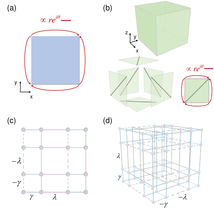
Figure 1: (a-b) Schematic for corner twisted boundary condition. In 2D square lattices, red arrows indicate the tunneling from one corner to the other, which are parametrized by $r\in[0,1]$ and $\theta\in[0,2\pi]$. In 3D cubic lattices, the CTBC is imposed on each face, with the dashed line indicating the orientation of the twist angle. (c-d) 2D and 3D Benalcazar-Bernevig-Hughes model under OBC. The tunneling amplitudes $\gamma$ and $\lambda$ are marked by different colors. The dashed lines represent negative amplitudes.

To meet the aforementioned criteria, we consider a corner twisted boundary condition (CTBC) shown in Fig. 1 (a-b), in which particles are allowed to tunnel between corners with a complex amplitude. In 2D square lattices, we adopt the CTBC [32]. In 3D cubic lattices, we consider the corner tunneling in each face of the cube, in which the orientation of the CTBC is implied by the dashed line. The CTBC is equivalent to threading a gauge field, resembling the general TBC. This choice of gauge field ensure that it will not significantly change the spectrum, which is confirmed by perturbative analysis later. To manifest the bulk-corner correspondence, the tunneling strength between corners is required to multiply a factor $r\in[0,1]$. With these conditions, we can define the MWN via Eq. (1). In addition, the CTBC can be used to define the multipole polarization [32], which is quantized by the chiral symmetry [24, 25] (see details in Supplemental Material [33] ).

Benalcazar-Bernevig-Hughes model. To illustrate the validity of our MWN, we consider the Benalcazar-Bernevig-Hughes (BBH) model [34] (see Fig. 1 (c-d)). This model preserves chiral symmetry and exhibits zero-energy corner states from higher-order topology. Notably, the BBH model with long-range tunneling has been realized in experiments [26]. In 2D, the system obeys the tight-binding Hamiltonian: ${{\hat{H}}_{{\rm{2D}}}}=-\sum\nolimits_{x,y}{\left[{{t_{x}}\hat{a}_{x+1,y}^{\dagger}{{\hat{a}}_{x,y}}+{{\left({-1}\right)}^{x}}{t_{y}}\hat{a}_{x,y+1}^{\dagger}{{\hat{a}}_{x,y}}}\right]}+{\rm{H}}.{\rm{c}}$, with ${t_{x}}=\frac{{\gamma+\lambda}}{2}+\frac{{\gamma-\lambda}}{2}{\left({-1}\right)^{x}},{t_{y}}=\frac{{\gamma+\lambda}}{2}+\frac{{\gamma-\lambda}}{2}{\left({-1}\right)^{y}}$. It is known that there are two topological phases determined by the ratio $|\gamma/\lambda|$. If $|\gamma/\lambda|<1$, a non-zero bulk multipole polarization arises and zero-energy modes emerge at corners under the OBC. Otherwise, if $|\gamma/\lambda|>1$, the system is well gapped and there is no in-gap zero modes. From the multipole polarization under periodic boundary condition (PBC), the phase boundary can be given as $|\gamma/\lambda|=1$. Under the CTBC, we calculate the spectrum and the MWN, see Fig. 2. Interestingly, the phase boundary deviates from $\gamma/\lambda=1$ due to the finite-size effect. Instead, the MWN correctly captures the gap closing point under the CTBC. The localization length of corner states near the phase transition point becomes significantly large, leading to hybridization of corner states and resulting in a non-zero energy shift. Thus, the phase transition point given by the MWN is also shifted. However, in the thermodynamic limit $L\to\infty$, the phase transition point approaches to $\gamma/\lambda=1$, see the inset in Fig. 2 (b). This phenomenon can by accounted by the topological obstruction between PBC and OBC [35].

Subsequently, we calculate the lowest singular value $\min({\Sigma})$ and the determinant $\det h(r,\theta)$ as functions of $r$ and $\theta$, see the right panel of Fig. 2. The lowest singular value of $h(r,\theta)$ corresponds to the eigenenergy most close to $E=0$. For $|\gamma/\lambda|<1$ (and away from the phase transition point), we confirm that there appears $2$ ($4$)-fold degenerate singular points at $r=0$ in the 2D (3D) BBH model. This is precisely captured by the MWN. Near the phase transition point, the singular point gradually move out of the integral circle, causing a zero MWN.

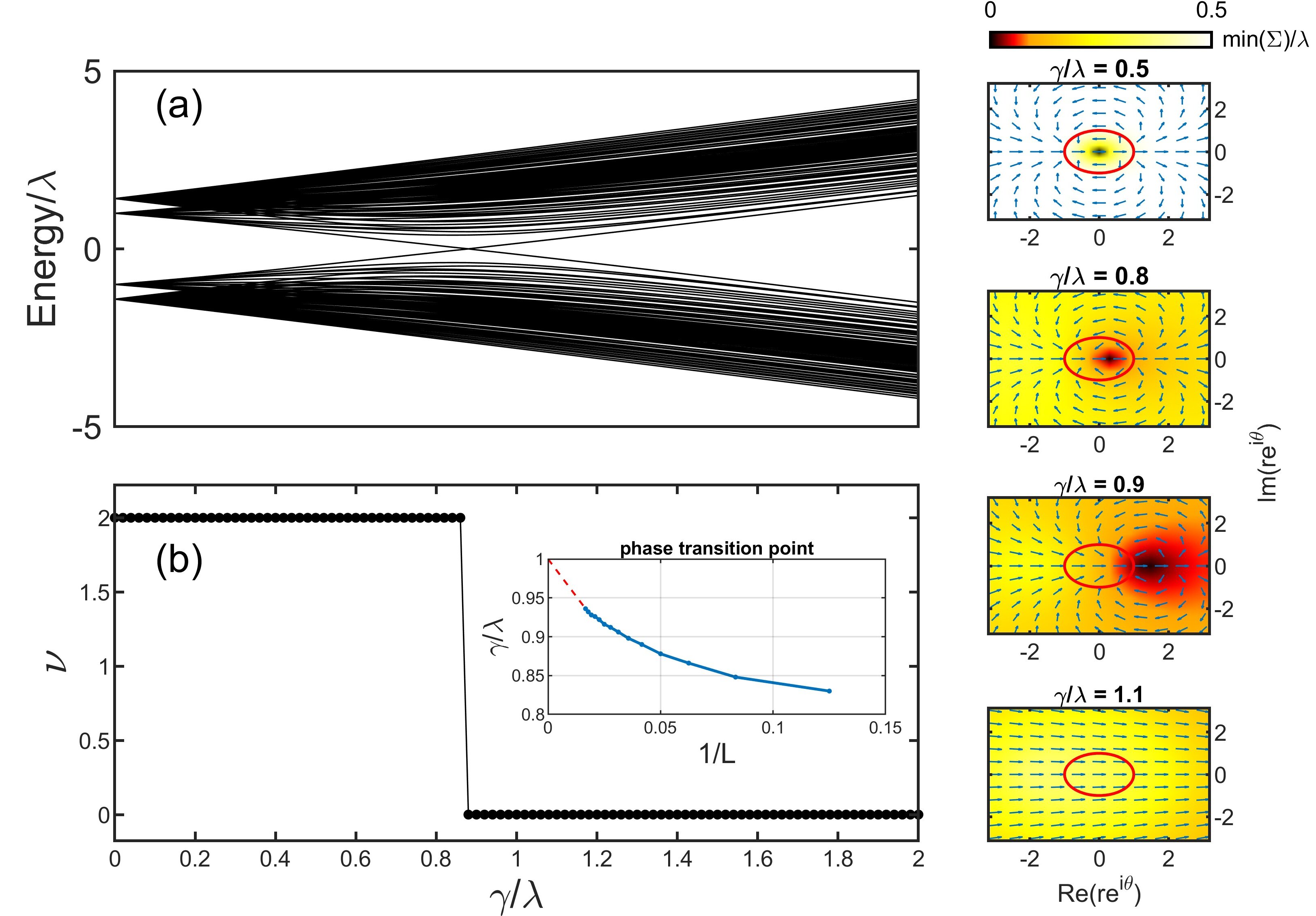
Figure 2: (a) Spectrum and (b) MWN of the 2D BBH model versus $\gamma/\lambda$ under the CTBC. Inset in (b): the critical $\gamma/\lambda$ versus $1/L$ with a red dashed line for guidance. Right panel: the lowest singular values $\min(\Sigma)$ of $h(r,\theta)$ on the complex plane for $L=20$. Arrows represent the angle of $\det h(r,\theta)$.

Real-space representation of multipole winding number. Below we show how to derive the real-space formulation for the MWN. The central idea is to make use of the gauge freedom of the CTBC and find appropriate gauges that makes the twist angle distributed uniformly in the bulk. Then the twist angle can be treated as a perturbation in order of $\theta/L$ and one can use the perturbative expansion to derive the MWN. To perform the gauge transformation, we introduce the twist operators

$$\hat{U}_{\theta}^{\mathrm{2D}}=\exp\left({i\frac{\theta}{L}{{\hat{\cal P}}_{xy}}}\right)~{}\textrm{with}~{}{\hat{\cal P}_{xy}}=\sum\limits_{x,y}{|x-y|{{\hat{n}}_{x,y}}}$$ (2)

for 2D systems and

$$\hat{U}_{\theta}^{\mathrm{3D}} = \exp\left({i\frac{\theta}{L}{{\hat{\cal P}}_{xyz}}}\right)~{}\textrm{with}~{}{{\hat{\cal P}}_{xyz}}=\sum\limits_{x,y}{{f_{xyz}}{{\hat{n}}_{x,y}}},$$

$${f_{xyz}} = \left\{{\begin{array}[]{*{20}{c}}{|x-y|-z+1,}&{|x-y|\geq z-1}\\ {|L-x-y|+z-L,}&{|L-x-y|\geq L-z}\\ {0}&{{\rm{otherwise}}}\end{array}}\right.$$ (6)

for 3D systems. Through the transformation $\tilde{H}\left(\theta\right)=\hat{U}_{\theta}\hat{H}\left(\theta\right){{\hat{U}_{\theta}}^{-1}}$, the gauge fields at corners are transformed into the bulk with diluted and uniform strength (see details in Supplemental Material [33]). The Hamiltonian $\hat{H}\left(\theta\right)$ under the CTBC satisfies the gauge-invariant relation: $\hat{H}\left({\theta+2\pi}\right)=\hat{H}\left(\theta\right)$, while the transformed Hamiltonian satisfies the covariant relation: $\tilde{H}\left({\theta+2\pi}\right)={{\hat{U}}_{2\pi}}\tilde{H}\left(\theta\right){{\hat{U}}_{2\pi}}^{-1}$. For simplicity, we refer to the former one as “corner gauge” and to the latter as “bulk gauge”. Operators under the bulk gauge will be denoted by tilde sign: $h\to\tilde{h}$. Meanwhile, the twist angle (gauge field) will only cause a slight modification in the spectrum, which can be neglected in the thermodynamic limit.

Choosing $r=1$, under the bulk gauge, the MWN can still be expressed as Eq. (1). Keeping the terms up to the first order of $1/L$, we have $\tilde{h}\left(\theta\right)=h\left(0\right)+\frac{\theta}{L}{[{\frac{\partial}{{\partial\theta/L}}\tilde{h}\left(\theta\right)}]_{\theta=0}}+O\left({\frac{1}{{{L^{2}}}}}\right)$ and ${\rm{Tr}}[{h{{\left({r,\theta}\right)}^{-1}}{\partial_{\theta}}h\left({r,\theta}\right)}]\approx{\rm{Tr}}\{{{h^{-1}}\left(0\right){{[{{{\partial_{\theta}}}\tilde{h}\left(\theta\right)}]}_{\theta=0}}}\}$ being a constant. Therefore, the MWN can be given as $\nu\approx-i{\rm{Tr}}\{{{h^{-1}}\left(0\right){{[{{{\partial_{\theta}}}\tilde{h}\left(\theta\right)}]}_{\theta=0}}}\}$. Using $\tilde{h}\left(\theta\right)={\bm{\psi}}_{A}^{\dagger}\tilde{H}\left(\theta\right){{\bm{\psi}}_{B}}$, we have $\tilde{h}={\cal U}_{2\pi}^{A}\tilde{h}\left(0\right){({{\cal U}_{2\pi}^{B}})^{-1}}$ with ${{\hat{U}}_{2\pi}}=\exp({i2\pi\hat{\mathcal{P}}/L})$, where $\hat{\mathcal{P}}=\{\hat{\cal{P}}_{xy},\hat{\cal{P}}_{xyz}\}$ are both diagonal in the position basis. For simplicity, we define the projected twist operator matrices in the sector $\alpha=\{A,B\}$: ${\cal U}_{2\pi}^{\alpha}\equiv{\bm{\psi}}_{\alpha}^{\dagger}{{\hat{U}}_{2\pi}}{{\bm{\psi}}_{\alpha}}$. To ensure the gauge invariance, we impose the constraint $\det\tilde{h}\left({2\pi}\right)=\det\tilde{h}\left(0\right)$. Thus, we require ${\cal U}_{2\pi}\equiv{\cal U}_{2\pi}^{A}={\cal U}_{2\pi}^{B}$, which can be easily satisfied by setting an identical position for all sublattices within a unit cell. Up to the first order of $1/L$, we have ${\left[{{\partial_{\theta}}\tilde{h}\left(\theta\right)}\right]_{\theta=0}}\approx\frac{{\tilde{h}\left({2\pi}\right)-\tilde{h}\left(0\right)}}{{2\pi}}=\frac{{{\cal U}_{2\pi}h{{{{\cal U}_{2\pi}^{-1}}}}-h}}{{2\pi}}$. To gain higher accuracy, one may consider a higher-order finite difference (see details in Supplemental Material [33]). Then, a rather simpler real-space formula can be obtained: $\nu=\frac{1}{{2\pi i}}{\rm{Tr}}\left({{h^{-1}}{\cal U}_{2\pi}h{{{{\cal U}_{2\pi}^{-1}}}}-I}\right)$. This leads to two equivalent real-space formulas: (i) the Bott index form and (ii) the non-commutative form.

Since ${{h^{-1}}{\cal U}_{2\pi}h{{{{\cal U}_{2\pi}^{-1}}}}}$ is close to an identity matrix, in the thermodynamic limit $L\to\infty$, one can obtain the Bott index form $\nu=\frac{1}{{2\pi i}}{\rm{Tr}}\left[{\log\left({{h^{-1}}{\cal U}_{2\pi}h{{{{\cal U}_{2\pi}^{-1}}}}}\right)}\right]$. This formula is analogous to the multipole chiral number [23], which also takes the Bott index form. The multipole chiral number is defined based on the quadrupole and octupole of polarization. It can be proved that the multipole chiral number is equivalent to the real-space winding number defined through a modified CTBC. The modified CTBC still connects the corners, while only those tunnelings related to one of the corners are threaded by a twist angle. In this scenario, the modified MWN captures the number of zero-energy modes induced in one specific corner (see details in Supplemental Material [33]). Therefore, although the generators of the twist operators [Eq. (2) and Eq. (Probing Chiral-Symmetric Higher-Order Topological Insulators with Multipole Winding Number)] are quite different from the quadrupole and octupole, they share the same physical origin.

Using the Baker-Campbell-Hausdorff (BCH) formula, we have ${{\cal U}_{2\pi}}h{{\cal U}_{2\pi}^{-1}}\approx h+2\pi i\left[{P,h}\right]/L$ with $P={\bm{\psi}}_{A}^{\dagger}\hat{\mathcal{P}}{\bm{\psi}}_{A}$ denoting the generator projected onto the sector $A$, and then obtain the non-commutative form $\nu=\frac{1}{L}\mathrm{Tr}\left({h^{-1}}\left[{{{P}},h}\right]\right)$. However, this approximation only holds for systems with OBC and $L\to\infty$. In a finite system with CTBC, this approximation is poor because it always evaluates to zero if $h$ is invertible: ${\rm{Tr}}\left({{h^{-1}}\left[{P,h}\right]}\right)={\rm{Tr}}\left({{h^{-1}}Ph-P}\right)=0$. This issue arises from the slow convergence of the BCH formula and the omission of higher-order terms (see details in Supplemental Material [33]). Meanwhile, as the CTBC connects the corners, general definition of the position near the corner become ill-defined, which also leads to the poor performance of the first-order expansion. However, under the OBC, the BCH formula converges fast because position-dependent operators are well-defined. In the presence of zero modes, $h$ becomes singular. In this case, we need to rule out the zero singular values and the associated vectors and use the pseudo-inverse formulation: $h^{-1}\approx\tilde{u}_{B}\tilde{\Sigma}^{-1}\tilde{u}_{A}^{{\dagger}}$ and then the non-commutative form will be non-zero.

Measurement of multipole winding number. The above forms for MWN are not straightforward to be measured in experiments. Below we derive a formula suitable for experimental measurement. Firstly, the flattened Hamiltonian can be written as $\hat{Q}={{\hat{\mathbb{P}}}_{+}}-{{\hat{\mathbb{P}}}_{-}}$ with ${{\hat{\mathbb{P}}}_{-}}=\sum\nolimits_{{E_{n}}<0}{|{\psi_{n}}\rangle\langle{\psi_{n}}|}$ and ${{\hat{\mathbb{P}}}_{+}}=\sum\nolimits_{{E_{n}}>0}{|{\psi_{n}}\rangle\langle{\psi_{n}}|}$, where $E_{n}$ is the eigenenergy for the eigenstate $|\psi_{n}\rangle$. The flattened Hamiltonian shares the same eigenstates of the original Hamiltonian and the zero-energy mode is naturally excluded. Replacing the off-diagonal matrix $h$ with the flattened matrix $q\equiv{\bm{\psi}}_{A}^{\dagger}\hat{Q}{{\bm{\psi}}_{B}}$ and $q^{-1}\equiv{\bm{\psi}}_{B}^{\dagger}\hat{Q}{{\bm{\psi}}_{A}}$, we have $\nu=\frac{1}{L}\mathrm{Tr}\left({q^{-1}}\left[{{{P}},q}\right]\right)$. Therefore, we obtain a real-space formula (see details in Supplemental Material [33]),

$$\nu=\frac{1}{L}\sum\limits_{{E_{n}}\neq 0}{\langle{\psi_{n}}|\hat{\Gamma}\hat{\cal P}|{\psi_{n}}\rangle},$$ (8)

which works well under OBC. With Eq. (8), we can extract the MWN by measuring the expectations of $\hat{\Gamma}\hat{\cal P}_{xy}$ for 2D systems or $\hat{\Gamma}\hat{\cal P}_{xyz}$ for 3D systems.

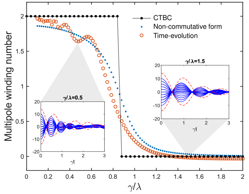
Figure 3: MWN obtained from the CTBC [Eq. (1)] (black dots), the non-commutative form [Eq. (8)] (blue dots), and the time-evolution [Eq. (11)] (red circles). Bulk initial states are chosen as Fock states ranging from $[L/3,2L/3]\times[L/3,2L/3]$. For initial states on the edge, we find it is sufficient to use four Fock states localized at the center of the edge: $(1,L/2),(L/2,1),(L,L/2),(L/2,L)$. Insets: the time-evolution of $\langle\Psi(t)|\hat{\Gamma}\hat{\cal P}_{xy}|\Psi(t)\rangle$ with the red dashed lines for the edge state and the blue lines for the bulk state. The system size is chosen as $30\times 30$, and the total evolution time is set as $\gamma t=3$.

In practice, one may use dynamical average to obtain the expectation over eigenstates. Below we show how to measure the MWN for a 2D BBH model. Under the CTBC, it can be found that there are boundary states localized near the four sides with non-zero energy. Hence, the MWN should not only relate to the bulk states, but also the boundary states. To attain Eq. (8), contributions from bulk and boundary states should be both taken into account. The numbers of boundary and bulk states are roughly $N_{\mathrm{edge}}=4L$ and $N_{\mathrm{bulk}}=L^{2}-4L$. We consider two kinds of initial states: the edge initial state $|{\Psi_{\mathrm{edge}}}\left(0\right)\rangle=\sum\nolimits_{\psi_{n}\in\mathrm{edge}}{{b_{n}}|{\psi_{n}}\rangle}$ and the bulk initial state $|{\Psi_{\mathrm{bulk}}}\left(0\right)\rangle=\sum\nolimits_{\psi_{n}\in\mathrm{bulk}}{{a_{n}}|{\psi_{n}}\rangle}$. Based upon the time-evolution from these initial states, one can obtain the contribution from the bulk

$${\nu_{\mathrm{bulk}}} = \frac{1}{{\Delta t}}\int_{t}^{t+\Delta t}{\langle{\Psi_{\mathrm{bulk}}}\left(t\right)|\hat{\Gamma}{{\hat{\cal P}}_{xy}}|{\Psi_{\mathrm{bulk}}}\left(t\right)\rangle\mathrm{d}t}$$ (9)

$$\approx \sum\nolimits_{\psi_{n}\in\mathrm{bulk}}{|{a_{n}}{|^{2}}\langle{\psi_{n}}|\hat{\Gamma}{{\hat{\cal P}}_{xy}}|{\psi_{n}}\rangle},$$

and the contribution from the edge

$${\nu_{\mathrm{edge}}} = \frac{1}{{\Delta t}}\int_{t}^{t+\Delta t}{\langle{\Psi_{\mathrm{edge}}}\left(t\right)|\hat{\Gamma}{{\hat{\cal P}}_{xy}}|{\Psi_{\mathrm{edge}}}\left(t\right)\rangle\mathrm{d}t}$$ (10)

$$\approx \sum\nolimits_{\psi_{n}\in\mathrm{edge}}{|{b_{n}}{|^{2}}\langle{\psi_{n}}|\hat{\Gamma}{{\hat{\cal P}}_{xy}}|{\psi_{n}}\rangle}.$$

For simplicity, we assume the initial state is a equal-weight superposition of its corresponding eigenstates, that is $|{a_{n}}{|^{2}}\approx\frac{1}{{{L^{2}}-4L}}$ and $|{b_{n}}{|^{2}}\approx\frac{1}{{4L}}$. Therefore, the MWN in Eq. (8) can be given as

$$\nu\approx\left({L-4}\right){\nu_{\mathrm{bulk}}}+4{\nu_{\mathrm{edge}}}.$$ (11)

Through numerical simulation, we check the validity of Eq. (11). We simulate the time-evolution from Fock states that localize at the center of the bulk and the edge, respectively. Then, we calculate $\nu_{\mathrm{bulk}}$ and $\nu_{\mathrm{edge}}$ to obtain the MWN via Eq. (11). These procedures are repeated for different Fock states chosen appropriately to ensure that all eigenstates except for the zero-energy modes are covered. By averaging them, we obtain the results in Fig. 3. The simulated results are consistent with the ones given by the non-commutative form Eq. (8). Note that it is difficult to achieve a very long time evolution in realistic experiments. In our scheme, it is sufficient to consider the evolution before states reach the corners, which avoids the influence of corner states (see details in Supplemental Material [33]).

Summary and Discussion. In summary, to characterize chiral-symmetric HOTIs, we have introduced the MWN and explored its experimental measurement. Through introducing suitable twist operators to transform the gauge field at corners into the bulk, the twist angle serves as a perturbation, leading to the derivation of a real-space formula for the MWN. This formula provides a practical approach for experimentally probing higher-order topology. Utilizing the corner twisted boundary condition, we demonstrate the effectiveness of the TBC-like method in computing real-space topological invariants.

In contrast to the conventional TBC, the CTBC exclusively connects corners, leading to the emergence of boundary states near borders in non-trivial cases. Notably, these boundary states have non-zero energies. The MWN is rooted in both bulk and edge contributions, setting it apart fundamentally from conventional chiral-symmetric topological insulators. This distinction necessitates measuring both contributions in experiments. Furthermore, the appearance of corner states is a consequence of the non-trivial topology of both the bulk and the edge. Thus, unlike the conventional topological band theory, the MWN can not be solely characterized with the Bloch states in bulk under the PBC.

In our real-space formulation, the twist operators [Eq. (2) and Eq. (Probing Chiral-Symmetric Higher-Order Topological Insulators with Multipole Winding Number)] significantly differ from the commonly used quadrupole and octupole [36, 37, 38, 24, 25]. This distinction arises from their connection to the topological invariant defined through specific TBC (see details in Supplemental Material [33]). Due to the gauge freedom, the twist operator is not unique, allowing for numerous gauge transformations and resulting in various possible real-space formulations using the introduced perturbative expansions. Despite these differences, they all share the same physical origin, underscoring the importance of the TBC method in studying real-space formulas for topological invariants. Moreover, the MWN defined through the CTBC effectively captures information about zero-energy modes. This enables the generalization of our method to a broad range of chiral-symmetric HOTIs beyond square or cubic structures, such as the honeycomb lattice [39, 40, 41, 42] and the kagome lattice [8, 43, 7]. The real-space formula for the corresponding MWN can be derived in a similar manner.