Boosting Column Generation with Graph Neural Networks
for Joint Rider Trip Planning and Crew Shift Scheduling

Abstract

Optimizing service schedules is pivotal to the reliable, efficient, and inclusive on-demand mobility. This pressing challenge is further exacerbated by the increasing needs of an aging population, the oversubscription of existing services, and the lack of effective solution methods. This study addresses the intricacies of service scheduling, by jointly optimizing rider trip planning and crew scheduling for a complex dynamic mobility service. The resulting optimization problems are extremely challenging computationally for state-of-the-art methods.

To address this fundamental gap, this paper introduces the Joint Rider Trip Planning and Crew Shift Scheduling Problem (JRTPCSSP) and a novel solution method, called AGGNNI-CG (Attention and Gated GNN- Informed Column Generation), that hybridizes column generation and machine learning to obtain near-optimal solutions to the JRTPCSSP with the real-time constraints of the application. The key idea of the machine-learning component is to dramatically reduce the number of paths to explore in the pricing component, accelerating the most time-consuming component of the column generation. The machine learning component is a graph neural network with an attention mechanism and a gated architecture, that is particularly suited to cater for the different input sizes coming from daily operations.

AGGNNI-CG has been applied to a challenging, real-world dataset from the Paratransit system of Chatham County in Georgia. It produces dramatic improvements compared to the baseline column generation approach, which typically cannot produce feasible solutions in reasonable time on both medium-sized and large-scale complex instances. AGGNNI-CG also produces significant improvements in service compared to the existing system.

Keywords: Mobility as a Service, Service Scheduling, Column Generation, Graph Neural Network

1 Introduction

Enhancing the efficiency, accessibility, equity, reliability, and safety of transportation systems is a critical research focus in both academia and industry. The burgeoning challenges of traffic congestion, environmental pollution from private vehicles, and the rigidity of traditional public transit systems, coupled with the needs of an aging population, have spurred the evolution of Mobility as a Service (MaaS). MaaS represents a significant shift from personal vehicle ownership towards a service-based mobility paradigm, facilitated by a unified platform that seamlessly integrates diverse transportation services from public and private entities (Smith, 2020; Mladenovic, 2021). In MaaS ecosystems, users can specify trip details such as origin, destination, timing, and preferences, and the system assembles a comprehensive travel plan, potentially combining on-demand shuttles, buses, and metro services. The system dispatches vehicles for on-demand components and guides users to appropriate lines and stops for fixed-route segments (see Figure 1 for a multimodal trip example in a MaaS framework).

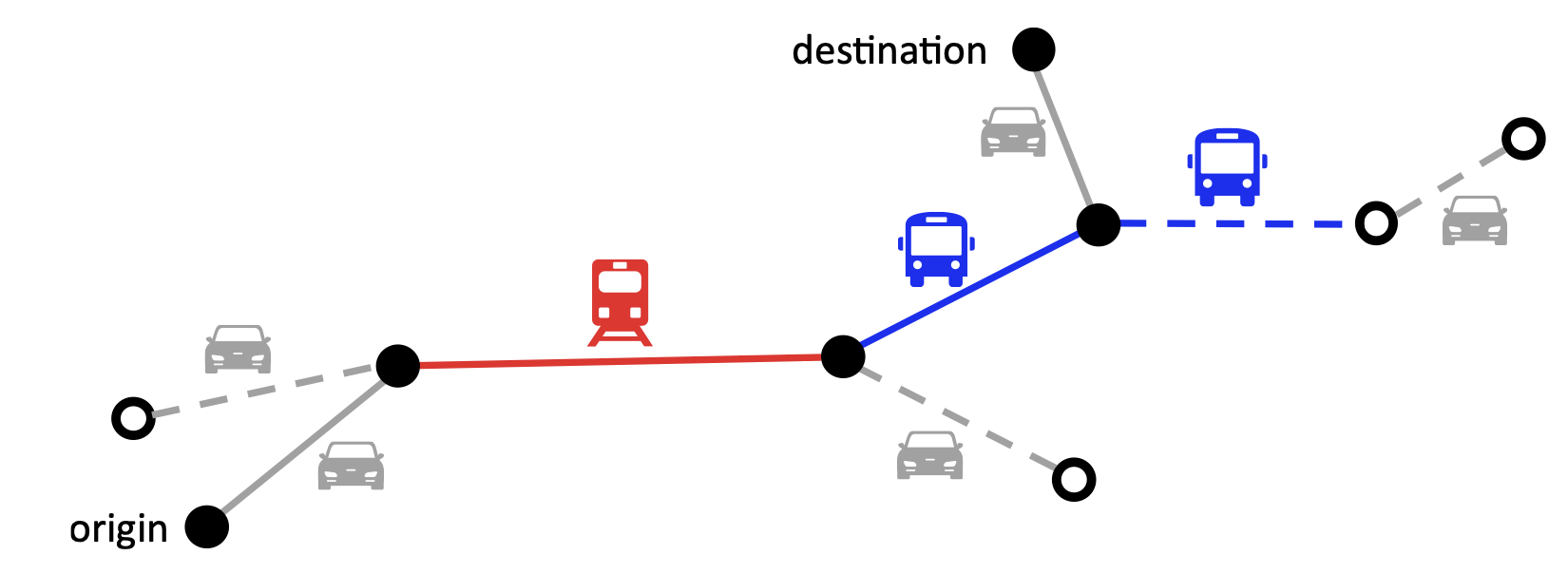
Figure 1: An example of a multimodal trip in MaaS systems, indicated by solid lines (adapted from (Auad et al., 2021))

The role of Paratransit operations within this evolving landscape is becoming increasingly crucial, particularly for achieving efficient and inclusive mobility. Paratransit services, traditionally designed to cater to riders unable to access standard transit services, are now facing unprecedented demand, particularly from an aging population. This surge in demand often results in oversubscribed operations, highlighting a critical need for more efficient and optimized service delivery. Moreover, these services, crucial for societal inclusivity, are typically costly and have historically suffered from suboptimal operational optimization. The integration of Paratransit with on-demand, real-time services is an emerging trend, further underscoring the need for advanced optimization techniques to manage the complexities of such integrated services.

Cities around the globe are actively experimenting with tailored MaaS solutions. For instance, Atlanta’s MARTA Reach pilot program, operational from March 1 to August 31, 2022, showcased an on-demand multimodal transit system (Van Hentenryck et al., 2023). Similarly, Sweden’s UbiGo began in Gothenburg in 2014 and expanded to Stockholm in 2016 (Smith et al., 2018), and Deutsche Bahn’s Qixxit in Germany offers nationwide journey planning and payment options across various modes of transport (Goodall et al., 2017).

Orchestrating optimal service schedules in MaaS systems, particularly in Paratransit operations, remains a formidable challenge. It requires a delicate balance between operational efficiency and user satisfaction, demanding strategic coordination of crew shifts and rider itineraries. The inherent combinatorial complexity of such scheduling tasks grows exponentially with the size of the problem, posing significant scalability challenges in practical implementations.

This paper, therefore, aims to explore whether the integration of machine learning and optimization can effectively address the computational challenges inherent in service scheduling within MaaS systems. We propose a novel hybrid approach that combines column generation with graph neural networks for the joint optimization of rider trip and crew schedules. This fusion of machine learning and optimization techniques is empirically validated using a real-world dataset, demonstrating significant improvements over existing methods. The findings suggest that our approach could be applied to optimize various MaaS operations, further contributing to the evolution of efficient and inclusive mobility solutions.

1.1 Related Work

1.1.1 Service Scheduling in MaaS Systems

Service scheduling in MaaS systems concerns both the rider and the crew sides, which correspond to the rider trip plan scheduling and the crew shift scheduling, respectively. In the literature, both have been extensively investigated, due to their importance in real-life operations.

For rider trip plan scheduling, the objective is to generate an optimal travel plan that fulfill the travel needs of a rider from origin to destination. A travel plan may consist of multiple travel segments, each of which is specified by travel mode, departure time, arrival time, and other information. Of course, rider trip requests are fulfilled by drivers/vehicles, especially in on-demand transportation systems. Therefore, trip plan scheduling is highly correlated with driver/vehicle tasks, i.e., at what time to serve which riders in what order. In the literature, the type of problem is typically modeled as dial-a-ride problem (DARP), which is a variant of the general vehicle routing problem. Readers are referred to for a comprehensive review of the DARP by Cordeau and Laporte (2007) and Ho et al. (2018). Solution methods in the existing studies can be classified into two classes: exact methods such as branch-and-cut (Cordeau, 2006; Ropke et al., 2007), branch-and-price (Garaix et al., 2010, 2011), and branch-and-price-and-cut algorithm (Qu and Bard, 2015; Gschwind and Irnich, 2015); heuristics such as tabu search (Cordeau and Laporte, 2003; Kirchler and Calvo, 2013), simulated annealing (Braekers et al., 2014), large neighborhood search (Ropke and Pisinger, 2006; Gschwind and Drexl, 2019; Jain and Hentenryck, 2011), and genetic algorithm (Jorgensen et al., 2007; Cubillos et al., 2009). In general, exact methods take longer time to produce high-quality solutions with bound information, while heuristics usually generate relatively good solutions without bound information within a shorter time. In the literature, most studies use either exact methods or heuristics; few study combines exact methods and heuristics in solving DARP.

For crew shift scheduling in public transit systems, a key challenge is the driver shift scheduling, whose objective is to design optimal driver shifts based on driver availability and time-varying rider travel needs in such a way that supply and demand are matched over time. The literature on driver scheduling in public transportation systems primarily focuses on traditional fixed-route systems (e.g., buses) and several key areas of research and methodological developments. Notable studies include exploring genetic algorithms for shift construction (Wren and Wren, 1995), defining efficient driver scheduling methodologies (Tóth and Krész, 2013), and integrating vehicle and crew scheduling with driver reliability (Andrade-Michel et al., 2021). Further research delves into robust and cost-efficient resource allocation for vehicle and crew scheduling, addressing operational disruptions (Amberg et al., 2019), and developing new mathematical models for the Drivers Scheduling Problem (DSP) that accurately reflect real-world complexities (Portugal et al., 2009). Studies also extend to addressing scheduling problems with mealtime windows and employing Integer Linear Programming (ILP) models for effective scheduling (Kang et al., 2019), and integrating duty scheduling and rostering to enhance driver satisfaction in public transit (Borndörfer et al., 2017). However, there is a notable gap in research focusing on emerging on-demand transit systems, as most studies primarily concentrate on conventional fixed-route bus systems, leaving room for exploration in the context of modern, demand-responsive transport models.

1.1.2 Machine Learning for Combinatorial Optimization

The integration of machine learning techniques to address combinatorial optimization problems has become an increasingly prominent field of study in recent years and it is impossible to make justice to the field in this section. Interested readers can referred to comprehensive reviews of recent progress by Bengio et al. (2021), Karimi-Mamaghan et al. (2022), and Mazyavkina et al. (2021). Research endeavors in this domain generally fall into one of two categories: the application of standalone machine learning models to derive solutions for combinatorial problems and the enhancement of traditional mathematical optimization methods through machine learning.

In the former category, a neural network is often engineered to discern the patterns linking problem instances to their optimal solutions. This process may involve learning from a dataset of existing solutions - a supervised learning approach (e.g., Vinyals et al. (2015)) - or discovering strategies through a process of trial and error, akin to reinforcement learning (e.g., Nazari et al. (2018)) or both as in Yuan et al. (2022a). The goal is to train machine learning models in a sufficiently robust manner to generate solutions autonomously. Despite the progress, achieving high-quality solutions solely with machine learning remains a challenging frontier. Combinatorial optimization problems are inherently complex and encompass vast solution spaces that are difficult to navigate efficiently. As a result, while machine learning models have shown promise, they often struggle to match the solution quality of established optimization methods. Recent studies underscore the persistent difficulty in bridging this quality gap, suggesting the need for more sophisticated models and training techniques.

In the latter category, machine learning models, once adequately trained, are often employed to streamline or assist with the most time-intensive aspects of traditional mathematical optimization methods. This can involve pivotal tasks such as choosing cutting planes in branch-and-cut algorithms or selecting columns in branch-and-price algorithms. By synergizing the strengths of both mathematical optimization and machine learning, this hybrid approach has demonstrated considerable promise in tackling a range of complex problems. Specifically, in the realm of enhancing the column generation algorithm through machine learning techniques - a critical component in vehicle routing and service scheduling within MaaS systems - researchers have recorded notable advancements. Morabit et al. (2021) applied a learned model to select promising columns from those generated at each iteration of column generation to reduce the computing time of reoptimizing the restricted master problem. Shen et al. (2022) designed an ML model to predict the optimal solution of pricing subproblems, which is then used to guide a sampling method to efficiently generate high-quality columns.

Further advances in this field involve using machine learning to streamline pricing subproblems. Pioneering studies have employed machine learning techniques to simplify underlying graphs, thereby lessening the complexity of these subproblems. Morabit et al. (2023) utilized a random forest model to predict edges likely to be part of the master problem’s solutions. Owing to the complexity and variable sizes of the graphs in subproblems, their model bases its predictions on local rather than global graph information. In addressing varying graph sizes, Yuan et al. (2022b) developed a graph neural network model with residual gated graph convolutional layers, inspired by Joshi et al. (2019). Their model evaluates the likelihood of each edge being part of the final solution, leading to the construction of a reduced graph that retains edges with higher predicted probabilities for pricing subproblems. The method proposed in this paper differs from Yuan et al. (2022b) in three key ways: First, this study tackle both crew shift scheduling and rider trip planning, unlike Yuan et al. (2022b) which focused only on the former. Second, the proposed method is applied to considerably larger and more complex real-world scenarios, whereas Yuan et al. (2022b) tested their algorithm on instances of smaller scales. Third, contrary to Yuan et al. (2022b), the the proposed machine learning model avoids updating the edge embeddings in each layer, a process that is computationally inefficient for larger scales. Instead, the proposed model integrates graph attention and residual gating mechanisms, incorporating edge-level features in the attention weight calculations without the need to keep track of the edge embeddings.

1.2 Motivations and Contributions

Despite notable progress in service scheduling in MaaS systems, several key challenges still require significantly more attention. First, there is a discernible need for an integrated framework that simultaneously addresses rider trip plans and crew shift scheduling. To date, within the academic sphere and in practice, these elements are predominantly examined in isolation, highlighting the necessity for a more holistic approach. Second, the inherent complexity of such an integrated routing and scheduling, especially in large-scale scenarios, poses significant computational challenges in order to generate high-quality solutions efficiently. Third, most existing studies evaluate their methods using synthesized datasets, leaving a void in capturing the realities in the field.

This study aims at addressing these challenges by introducing an integrated approach for the Joint Rider Trip Planning and Crew Shift Scheduling Problem (JRTPCSSP) for MaaS systems. Moreover, to address the computational challenges of the JRTPCSSP, the study combines a traditional column generation with an Attention-Based, Gated Graph Neural Network to reduce the search space and find high-quality solutions quickly. More precisely, the primary contributions of this research can be summarized as follows:

• This study introduces the JRTPCSSP that concurrently optimizes rider trip plans and crew shifts, leveraging large joint search spaces to potentially enhance both rider experience and system operational efficiency.

• To tackle the complexity of the JRTPCSSP, this study fuses machine learning and column generation. The key idea of the machine-learning component is to dramatically reduce the number of paths to explore in the pricing component, effectively accelerating the most time-consuming component of the column generation. In particular, the machine-learning model learns which edges are likely to be present in high-quality solutions.

• To address the reality that each day of operation will feature different trip requests, the study uses a Graph Neural Network (GNN) that can smoothly adapt to inputs of variable sizes. Morover, the use of an attention mechanism and a gated architecture enables the machine learning model to finely tune the GNN.

• The resulting learning and optimization algorithm, called AGGNNI-CG (Attention and Gated GNN-Informed Column Generation), has been applied to a challenging, real-world dataset from the Paratransit system of Chatham County in Georgia. On scaled down instances, AGGNNI-CG is shown to (almost always) produce solutions of higher quality than the base column generation, often with order of magnitude reductions in computing time. On the actial dataset, AGGNNI-CG finds near-optimal solutions on all instances, while the baseline column generation almost never finds a feasible solution. Moreover, AGGNNI-CG is shown to significantly improve quality of service compared to the existing system.

The rest of this paper is organized as follows. Section 2 defines the JRTPCSSP. Section 3 presents the column generation. Section 4 describes the machine learning methodology and its use within the column generation. Section 5 reports the benefits of the proposed approach on the real-world dataset. Section 6 concludes the paper and discusses future research directions.

2 Joint Rider Trip Planning and Crew Shift Scheduling

2.1 Problem Description

The JRTPCSSP considered in this paper is a variant of the Dial-A-Ride Problem (DARP). Readers are referred to (Cordeau and Laporte, 2007) and (Ho et al., 2018) for comprehensive literature reviews on the DARP. Compared to the classic DARP, there are two additional features considered in the paper. First, the JRTPCSSP considers scenarios where a single rider may have multiple trip requests within the same day, and imposes a constraint of complete service: either all requests from a specific rider are fulfilled, or none at all. This approach prohibits partial servicing of a rider requests: it is motivated by the need to ensure a trip back (e.g., when a rider is a dialysis patient). Second, the JRTPCSSP imposes a maximum working duration for each driver (for example, 8 hours), but does not predetermine the driver shifts. For simplicity, the JRTPCSSP assumes a one-to-one correspondence between drivers and vehicles. Consequently, the terms “driver” and “vehicle” are used interchangeably throughout the paper.

Formally, the problem is defined as follows. Consider a set of riders, denoted as $U$, each associated with a set of trip requests $R_{u}$. These requests are to be accommodated by a homogeneous fleet of vehicles, denoted by $F$. Each trip request $r$ in $R_{u}$ has an origin $o_{r}$, a destination $d_{r}$, and time windows for both departure and arrival times. While it is not imperative to fulfill every trip request, it is crucial to note that partial servicing of an individual rider requests is not permissible: either all the requests in $R_{u}$ are served or none of them. Each vehicle $f$ in the fleet $F$ has a capacity of $C$, and the fleet size is constant at $\lvert F\rvert$. The working shifts of these vehicles are not predefined; instead, they need to be strategically determined alongside the scheduling of the trip requests. The maximum working hours of each vehicle is $l$. All vehicles initiate and conclude their service at a common depot, labeled $D$. The travel times between the depot, origins, and destinations are known and constant. The primary goal is to devise an optimal schedule for the vehicle working hours and the service of trip requests that maximizes the number of requests served. This objective is motivated by realities in the field, where the number of requests often exceeds the capacity of the service.

2.2 An Arc-Based Model

Figure 2 presents an arc-based model for the JRTPCSSP. The model is defined on the graph $G=(N,E)$, where $N$ denotes the set of nodes and $E$ the set of edges. Each trip request $r\in R$ is represented by a pickup node $i$ and a corresponding dropoff node $n+i$, included in the pickup node set $P$ and dropoff node set $D$, respectively, where $n=|R|$. Additionally, an origin depot node $0$ and a destination depot node $2n+1$ are created for the depot $D$, leading to the definition $N=\{0\}\cup P\cup D\cup\{2n+1\}$. The set $E$ comprises edges that connect nodes in $N$, subject to the satisfaction of time window constraints.

The binary decision variable $x_{ij}^{f}$ determines whether vehicle $f$ traverses edge $(i,j)$. For simplicity, $x^{f}(\delta^{+}(i))=\sum_{(i,j)\in E}x_{i,j}^{f}$ and $x^{f}(\delta^{-}(i))=\sum_{(j,i)\in E}x_{j,i}^{f}$ denote the sum of outgoing and incoming flows to node $i$, respectively, and $\delta^{+}(i)$ and $\delta^{-}(i)$ represent the sets of outgoing and incoming arcs of node $i\in N$. The objective function, defined in equation (2), aims at maximizing the number of trip requests served. In constraint (2), binary variable $y_{u}$ represents whether rider $u$ is served and the constraint links $y_{u}$ to flows from each pickup node $i\in P_{u}$, where $P_{u}$ denotes the set of pickup nodes associated with rider $u$. Constraint (2) prevents partial service. Constraint (2) enforces that pickup and dropoff services for each trip request are completed by the same vehicle. Constraint (2) ensures flow balance, and constraint (2) updates vehicle arrival times at each node, with $T_{i}^{f}$ as the arrival time of vehicle $f$ at node $i$, $s_{i}$ the service time at node $i$, and $t_{ij}$ the travel time from node $i$ to node $j$. Constraint (2) enforces time window requirements at node $i$, where $a_{i}$ and $b_{i}$ are the earliest and latest service start times, respectively. Constraint (2) specifies the maximum working hours of each driver. Constraint (2) updates the number of riders in vehicle $f$ after visiting node $j$, denoted as $Q_{j}^{f}$, with $d_{i}$ representing the demand at node $i$. Constraint (2) specifies the bounds of $Q_{i}^{f}$. Lastly, constraints (2) and (2) define the domains of the decision variables.

∑_f ∈F ∑_i ∈P x^f(δ^+(i)) ∑_f ∈F x^f(δ^+(i)) = y_u   ∀u ∈U, ∀i ∈P_u x^f(δ^+(i)) - x^f(δ^+(n+i)) = 0   ∀i ∈P, ∀f ∈F x^f(δ^+(i)) - x^f(δ^-(i)) = {1 if i = 0-1 if i=2n+10 i ∈P ∪D   ∀i ∈N, ∀f ∈F (T^f_i + s_i + t_ij)x^f_ij ≤T^f_j   ∀(i,j) ∈E, ∀f ∈F a_i ≤T^f_i ≤b_i   ∀i ∈N, ∀f ∈F T_2n+1^f - T_0^f ≤l   ∀f ∈F (Q^f_i + d_j)x^f_ij ≤Q^f_j   ∀(i,j) ∈E, ∀f ∈F max(0,d_i) ≤Q^f_i ≤min(C,C+d_i)   ∀i ∈N, ∀f ∈F x^f_ij ∈{0,1}   ∀(i,j) ∈E, ∀f ∈F y_u ∈{0,1}   ∀u ∈U

Figure 2: The Arc-Based Model.

2.3 A Path-Based Model

State-of-the-art solvers are not capable of solving large-scale instances encountered in practice using the arc-based formulation presented in Section 2.2. Instead, AGGNNI-CG is based on a path-based model presented in Figure 3. On many practical applications, the path-based formulation can leverage column generation to find high-quality solutions more efficiently, as demonstrated by prior studies (e.g., Riley et al. (2019); Lu et al. (2022)).

∑_r ∈R y_r y_r ≤∑_θ∈Ω α_rθλ_θ  ∀r ∈R y_r = y_r’   ∀u ∈U, ∀(r,r’) ∈{(r,r’)—r ∈R_u, r’ ∈R_u, r ≠r’} ∑_θ∈Ω λ_θ ≤—F—   λ_θ ∈{0,1}   ∀θ∈Ω y_r ∈{0,1}   ∀r ∈R

Figure 3: The Path-Based Model.

The objective function, defined in equation (3), aims at maximizing the number of fulfilled trip requests. The binary variable $y_{r}$ indicates whether a trip request $r$ is served. The set $R=\bigcup_{u\in U}R_{u}$ encompasses all trip requests. The term on the right-hand side of constraint (3) denotes whether request $r$ is served by the selected routes from the set $\Omega$. Here, $\alpha_{r\theta}$ represents whether request $r$ is served by route $\theta\in\Omega$, and binary variable $\lambda_{\theta}$ indicates whether route $\theta$ is selected in the routing solution. Constraint (3) ensures complete servicing of each rider requests without partial fulfillment. Constraint (3) controls the maximum number of vehicles that can be deployed. Lastly, constraints (3) and (3) define the domains for the decision variables $\lambda_{\theta}$ and $y_{u}$, respectively.

Each $\theta\in\Omega$ is a feasible vehicle route that satisfies constraints (2) to (2). Therefore, each vehicle route $\theta$, not only contains trip service schedules, but also provides driver shift information. The major challenge of solving model 3 is to find feasible routes and construct the route set $\Omega$. The size of set $\Omega$ increases exponentially with the number of trip requests. Hence, it is practically impossible to enumerate all routes in the set. Section 3 shows how to use column generation to iteratively add promising routes in the set $\Omega$ and avoid enumerating all routes.

3 The Column Generation Algorithm

3.1 Problem Decomposition based on Driver Shifts

As previously discussed, this goal of the JRTPCSSP is not only to design optimal trip service schedules but also to determine the driver shifts that best accommodate the time-varying travel demands from the riders. In practical operations, driver shifts typically commence at specific times (hourly or half-hourly) for management convenience. This observation underpins the initial step of AGGNNI-CG: the generation of the candidate set for driver shifts. It is important to emphasize that, in the solution, multiple drivers can use the same shifts and some shifts may not be used at all. It is the role of AGGNNI-CG to determine the best driver shifts to serve as many requests as possible.

For concreteness, consider a scenario with the earliest and latest service times denoted by $t_{s}$ and $t_{e}$, respectively, and a maximum driver working duration of $d$ hours. Assuming a time interval $\delta$ between adjacent shift candidates, the candidate set $\Phi$ for driver shifts can be defined as

$$\Phi={(dr_{s},dr_{e})|dr_{s}=t_{s}+k\delta,dr_{e}=dr_{s}+d,0\leq k\leq\lceil(t_{e}-t_{s}-d)/\delta\rceil,k\in\mathbb{Z}},$$ (1)

where each element $\phi=(dr_{s},dr_{e})\in\Phi$ represents a driver shift, with $dr_{s}$ and $dr_{e}$ indicating its start and end times, respectively. Figure 4 illustrates such a candidate set with parameters $t_{s}=5$, $t_{d}=22$, $d=8$, and $\delta=1$.

Figure 4: A Potential Candidate Set for Driver Shifts on a Particular Day.

For a given candidate set $\Phi$ of driver shift, the Restricted Linear Master Problem (RLMP) of AGGNNI-CG is presented in Figure 5. This model relaxes the integrality of of the decision variables $\lambda_{\theta}$ and $y_{r}$. Additionally, a restricted route set $\Omega_{\phi}^{\prime}$ is introduced for each driver shift candidate $\phi\in\Phi$: it contains a subset of feasible vehicle routes corresponding to driver shift $\phi$.

∑_r ∈R y_r y_r ≤∑_ϕ∈Φ ∑_θ∈Ω_ϕ’ α_rθλ_θ  ∀r ∈R y_r = y_r’   ∀u ∈U, ∀(r,r’) ∈{(r,r’)—r ∈R_u, r’ ∈R_u, r ≠r’} ∑_ϕ∈Φ ∑_θ∈Ω_ϕ’ λ_θ ≤—F—   λ_θ ∈[0,1]   ∀θ∈⋃_ϕ∈Φ Ω_ϕ’ y_r ∈[0,1]   ∀r ∈R

Figure 5: The Restricted Linear Master Problem.

For each $\Omega_{\phi}^{\prime}$, promising feasible routes using driver shift $\phi$ are iteratively added by solving the corresponding pricing subproblem. It is important to note that a finer granularity in the driver shift set $\Phi$, determined by $\delta$, does not substantially increase the complexity of identifying promising routes in these subproblems. This is because each subproblem is independent and can be processed in parallel. Furthermore, a higher number of subproblems potentially introduces more promising routes in each column generation iteration, which may reduce the total number of iterations required.

3.2 The Pricing Subproblem

∑_r ∈R π_r y_r -σ (2) - (2)

Figure 6: The Pricing Subproblem For Driver Shift $\phi$.

For each driver shift $\phi\in\Phi$, in each column generation iteration, new promising routes can be added to $\Omega_{\phi}^{\prime}$ by solving the pricing subproblem shown in Figure 6. In the objective function (6), $\pi_{r}$ and $\sigma$ denote the dual values of constraints (5) and (5) after solving Model (5). The pricing subproblem can be viewed as a shortest path problem with resource constraints. AGGNNI-CG uses dynamic programming method to solve the pricing problem. The implementation does not solve the pricing subproblem to optimality for each driver shift, which can be very time-consuming. Instead, AGGNNI-CG stops the dynamic programming process as soon as a certain amount of routes with negative reduced costs have been generated.

3.3 Finding Integer Feasible Solutions

The column generation often produces solutions that are be fractional, rendering them infeasible for the original model detailed in formulation (3). To derive integer solutions, the column generation algorithm is typically embedded within a branch-and-price framework. Two primary approaches are prevalent for branching strategies: edge-based and path-based. Edge-based branching tends to yield more balanced subproblems, whereas path-based branching is more efficient in rapidly identifying integer feasible solutions. However, preliminary experiments revealed that, given the high complexity and large scale of the problems in this study, neither exact edge-based nor path-based branching strategies could produce feasible solutions within a reasonable time frame. Consequently, AGGNNI-CG employs a path-based branching strategy complemented by a straightforward heuristic. Specifically, if the optimal solution of the RMLP is fractional, the variable associated with column with the highest $\lambda_{\theta}$ value is fixed to 1 and a new phase of the column generation algorithm is initiated. This process is repeated until an integer feasible solution is obtained.

4 Boosting Column Generation with Machine Learning

In the column generation method outlined in Section 3, the most computationally intensive components are the pricing subproblems, which are NP-hard themselved being shortest paths with resource constraints. To address this computational challenge, AGGNNI-CG leverages machine learning to speed up the resolution of the pricing subproblems.

4.1 The Machine Learning Framework

The machine learning framework of AGGNNI-CG is depicted in Figure 7. It is predicated on the observation that the trip demands tend to exhibit stable patterns over time in real-world settings. Consequently, insights gleaned from historical trip scheduling can inform and streamline future operations. The core strategy involves simplifying the graph structure for new instances by discarding edges unlikely to yield promising routes, drawing on patterns recognized from past solutions of pricing subproblems.

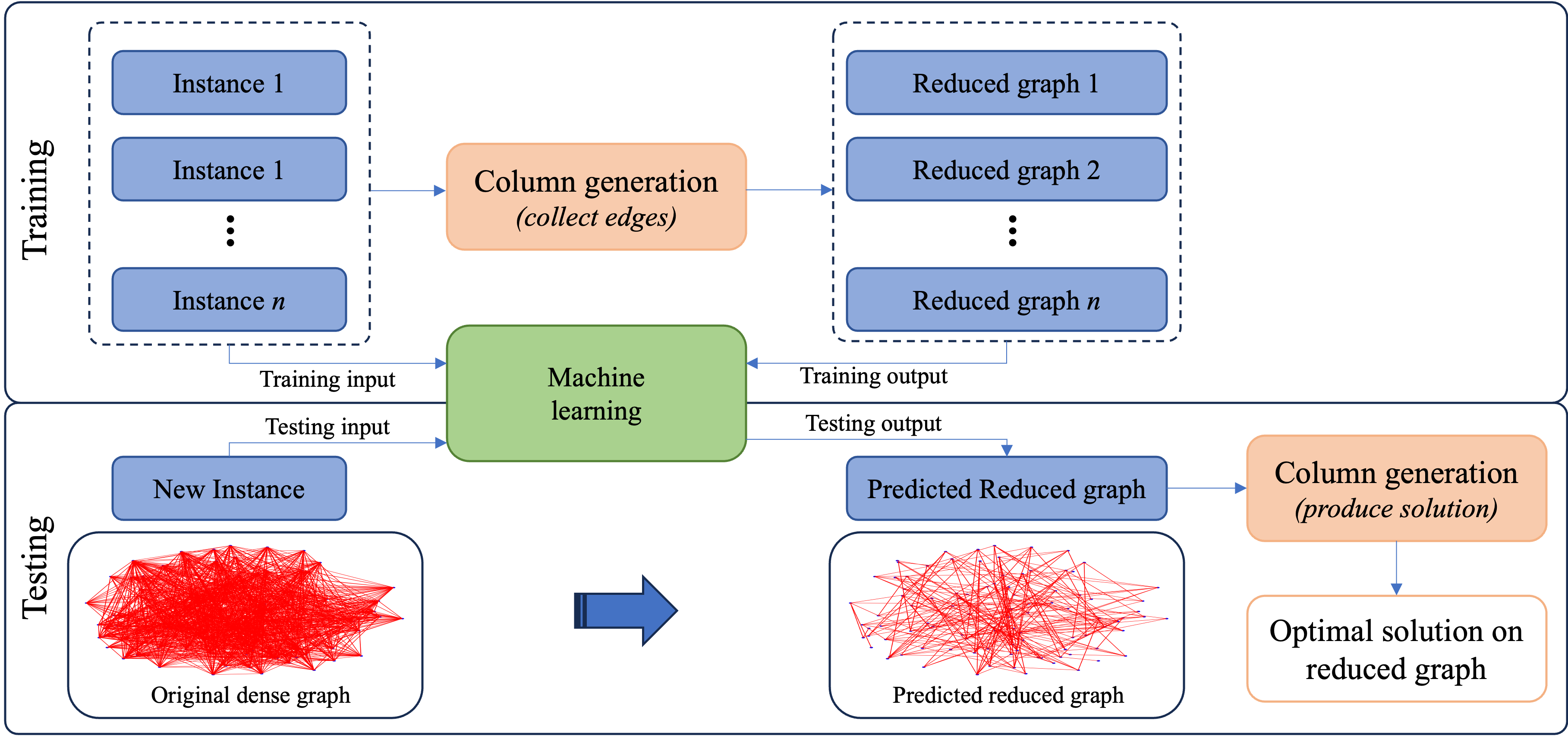
Figure 7: The Machine Learning Framework of AGGNNI-CG.

Initially, a dataset of historical instances is compiled, and the column generation algorithm from Section 3 is applied. Throughout this process, edges that frequently appear in the solutions of the restricted linear master problem across iterations are earmarked as promising. Upon completion of the column generation process, AGGNNI-CG constructs a reduced graph for each instance using these identified edges. It is important to note that the definition of “promising” extends beyond the edges present in the final solutions; it also encompasses those utilized in intermediate steps. This distinction is crucial for three reasons: first, the column generation algorithm in AGGNNI-CG incorporates heuristic elements, which implies that the obtained solutions may not necessarily represent the global optimum. Second, for most of real-world instances used in this study, due to the problem complexity, traditional column generation algorithm is even not able to produce a feasible solution. Third, focusing solely on the edges from final solutions could lead to infeasible problem formulations.

The machine learning model of AGGNNI-CG is trained on the historical instances and their respective reduced graphs. The learning goal is is to capture the underlying patterns correlating instances with their simplified graph representations.

For a new (unseen) instance, the trained model predicts a reduced graph, which is then used as the basis for solving the instance with column generation. The trimmed down graph, having fewer edges, enables the pricing subproblems to be solved more expeditiously, thereby significantly enhancing the efficiency of the overall column generation process.

4.2 Graph Neural Networks

AGGNNI-CG uses a GNN for predicting promising edges. In the realm of machine learning, GNNs belong to a class of deep learning models that stand out due to their ability to exploit the graph-based structure inherent in various problems. The GNNs processes each node based on its own features and those of its neighbors, which is done using shared weight parameters across all nodes in the graph (Kipf and Welling, 2016). This shared weight architecture uniquely positions GNNs to handle datasets of varying input and output dimensions, independent of the size of the graph. This feature is particularly important to the JRTPCSSP, because the number of requests varies, sometimes significantly from day to day, thereby leading to difference in the dimension of the graph instances. The cornerstone to GNN is its message passing mechanism, a sophisticated process where each node in the graph not only computes but also aggregates messages based on the attributes of its neighboring nodes. This dual-phase operation enables the GNN to intricately capture and integrate both local interactions and the broader structural context of the graph.

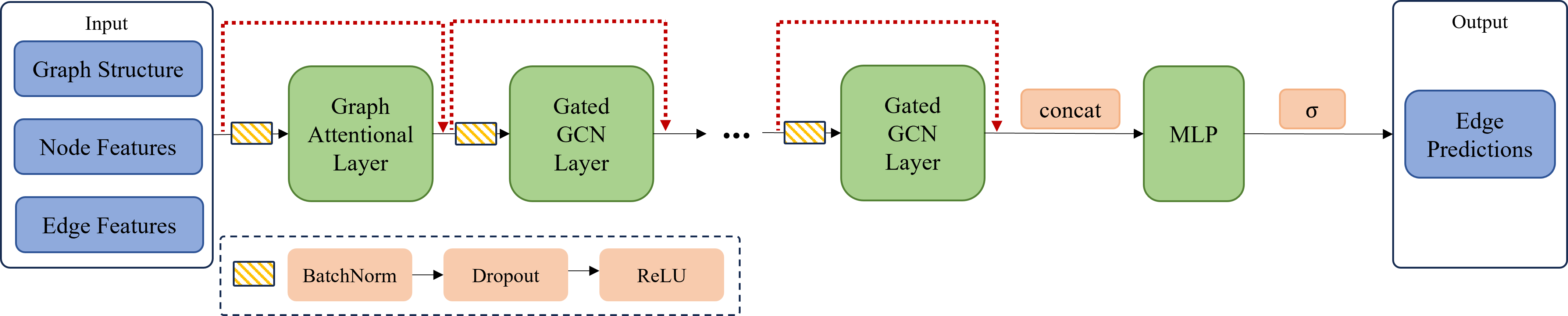
Figure 8: A diagram of the graph neural network pipeline for edge classification

The GNN-based pipeline of AGGNNI-CG to address the aforementioned edge-level classification problem is shown in Figure 8. The rest of this section covers each component in detail.

4.2.1 Features and Labels Encoding

For each graph instance $G=(N,E)$, AGGNNI-CG extracts features that represent the characteristics for each node $i\in N$. Specifically, the feature vector considered for node $i$ is $\left[\text{lat}_{i},\text{lon}_{i},a_{i},b_{i},\text{one-hot}(\{\text{pickup},\text{depot}\})\right]$. This vector comprises the node’s geographical coordinates (latitude and longitude), time window, and a one-hot encoded representation indicating whether the node corresponds to a pickup node (otherwise a drop-off node), or a depot node. In addition, AGGNNI-CG includes features $\left[t_{ij},\{1,0\}\right]$ for each edge $(i,j)\in E$, indicating the travel time from node $i$ to node $j$ and whether $(i,j)$ directly connects the origin and destination of the same trip. The labels $p_{ij}$ are produced by assigning a binary score to each edge $(i,j)$ in accordance with Section 4.1. Specifically, edges that are used at any time during the column generation algorithm are assigned the label $1$; otherwise, they receive the label $0$.

To ensure different features from different input instances fall into the same scale, AGGNNI-CG applies a minmax scaler that maps each feature into the range $[0,1]$ for every instance. The scaled node features are served as the initial node embeddings $\mathbf{h}_{i}^{0}$ for each node $i$, and the scaled edge features $\mathbf{e}_{ij}$ for each edge $(i,j)$ are merged into the node embeddings through the first graph convolutional layers.

4.2.2 The Graph Convolutional Layers

The node embeddings are first updated through one layer of the multi-head graph attenional operator (GATConv), the core of the Graph Attention Network (GAT) architecture from Brody et al. (2021); Veličković et al. (2017). In contrast to classical graph convolutional networks which employ equal-weight neighborhood aggregation for message passing, the multi-head attention mechanism in graph allows for the assignment of different weights to different neighbor nodes.

Taking the edge features into consideration, AGGNNI-CG computes the attention weight $\gamma_{ij}$ between a pair of nodes $i$ and $j$ as follows, which measures the significance of neighbor $j$’s embeddings to node $i$:

$$\gamma_{ij}=\frac{\exp{(\mathbf{a}^{\top}\text{LeakyReLU}(\mathbf{W}_{1}\mathbf{h}_{i}^{0}+\mathbf{W}_{2}\mathbf{h}_{j}^{0}+\mathbf{W}_{3}\mathbf{e}_{ij})})}{\sum_{k\in N(i)\cup\{i\}}\exp{(\mathbf{a}^{\top}\text{LeakyReLU}(\mathbf{W}_{1}\mathbf{h}_{i}^{0}+\mathbf{W}_{2}\mathbf{h}_{k}^{0}+\mathbf{W}_{3}\mathbf{e}_{ik}))}}$$ (2)

$$\text{LeakyReLU}(x)=\begin{cases}x&\text{if }x>0,\\ 0.2x&\text{if }x\leq 0.\end{cases},$$ (3)

where $N(i)$ corresponds to the set of neighbor nodes of node $i$; $\mathbf{a}$, $\mathbf{W}_{1}$, $\mathbf{W}_{2}$, and $\mathbf{W}_{3}$ are learneable parameters.

After obtaining the attention weights for each pair of nodes, AGGNNI-CG updates the node embeddings of each node $i$ by calculating the weighted sum of the transformed features of its neighbors:

$$\mathbf{h}_{i}^{1}=\gamma_{ii}\mathbf{W}_{1}\mathbf{h}_{i}^{0}+\sum_{j\in N(i)}\gamma_{ij}\mathbf{W}_{2}\mathbf{h}_{j}^{0}.$$ (4)

For multi-head attention with $H>1$ attention heads, the node embeddings should instead be updated by concatenating $H$ independent attention mechanisms following Equation 4:

$$\mathbf{h}_{i}^{1}=\mathop{\|}\limits_{g=1}^{H}\gamma_{ii}^{g}\mathbf{W}_{1}^{g}\mathbf{h}_{i}^{0}+\sum_{j\in N(i)}\gamma_{ij}^{g}\mathbf{W_{2}}^{g}\mathbf{h}_{j}^{0},$$ (5)

where $\mathop{\|}$ represents the concatenation operator, $\gamma_{ij}^{g}$ are the attention weights obtained from the $g$-th attention mechanism, and $\mathbf{W_{1}^{g}}$ and $\mathbf{W_{2}^{g}}$ are the corresponding learneable parameter matrices. Visualizations of the process within the graph attentional layer are shown in Figures 10 and 10.

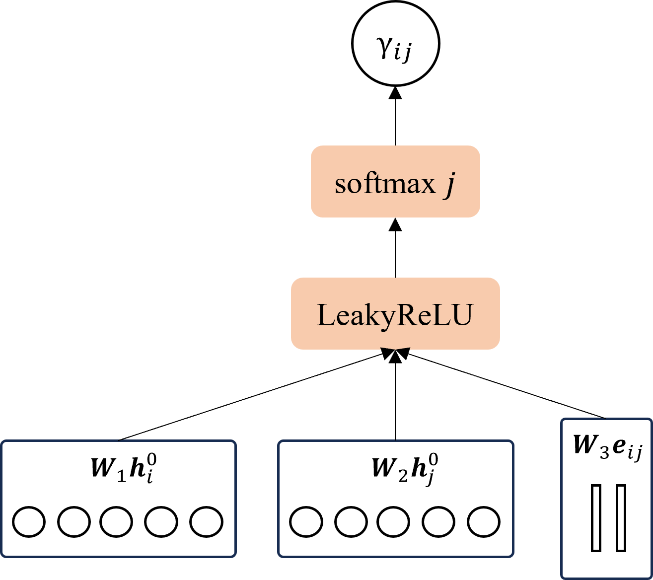
Figure 9: Visualization of the Attention Mechanism.

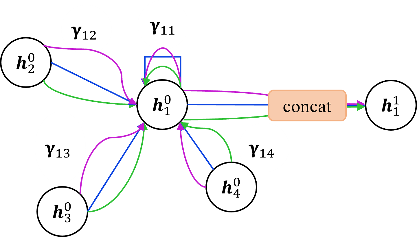
Figure 10: Visualization of Multi-Head Attention (with $H$ = 3 heads) by Node 1 on its Neighborhood; different arrow colors represent different attention heads; adapted from Veličković et al. (2017)

.

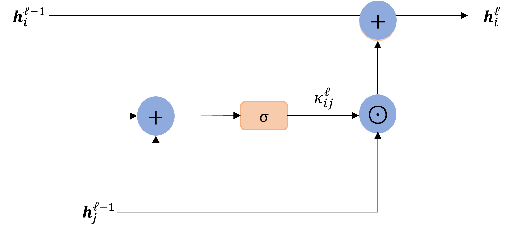
Figure 11: Visualization of the Gating Mechanism.

Subsequently, the node embeddings are fed into multiple layers of the Residual Gated Graph ConvNets (GCN), which has been used in several related studies (Joshi et al., 2019; Yuan et al., 2022b). The number of Residual Gated GCN layers is considered as a hyperparameter, which is fine-tuned during the experiments. For each layer $2\leq\ell\leq L$, the node embeddings are updated following a gating mechanism described in (Bresson and Laurent, 2017):

$$\mathbf{h}_{i}^{\ell}=\mathbf{\Theta_{1}}^{\ell}\mathbf{h}_{i}^{\ell-1}+\sum_{j\in N(i)}\kappa_{ij}^{\ell}\odot\mathbf{\Theta_{2}}^{\ell}\mathbf{h}_{j}^{\ell-1},$$ (6)

with the gate $\kappa_{ij}^{\ell}$ being:

$$\kappa_{ij}^{\ell}=\sigma(\mathbf{\Theta_{3}}^{\ell}\mathbf{h}_{i}^{\ell-1}+\mathbf{\Theta_{4}}^{\ell}\mathbf{h}_{j}^{\ell-1}),$$ (7)

where $\odot$ is the element-wise multiplication operator, $\mathbf{\Theta_{1}}^{\ell},\mathbf{\Theta_{2}}^{\ell},\mathbf{\Theta_{3}}^{\ell},\mathbf{\Theta_{4}}^{\ell}$ are learneable parameters for the $\ell$-th GCN layer, and $\sigma$ is the Sigmoid function. The gating mechanism is illustrated in Figure 11.

The model performance was enhanced by applying established methods to the node embeddings before they enter each graph convolutional layer. Batch normalization and dropouts stabilize training and prevent overfitting, while ReLU (the rectified linear unit) activation functions introduce non-linearities. Moreover, the GNN also incorporates skip connections to amplify the influence of the embeddings generated in the initial layers. This approach has shown empirical success in improving node differentiation within the model.

4.2.3 Edge-level Predictions Decoding

After the graph convolutional layers produce the final node embeddings, AGGNNI-CG transforms them into edge embeddings. This is achieved by concatenating the embeddings of the two nodes constituting each edge. These concatenated embeddings are then used as inputs into a Multi-layer Perceptron (MLP) layer and a Sigmoid function is applied to the output of MLP. This results in a predicted probability score $\hat{p}_{ij}$ for each edge. representing the likelihood that edge $(i,j)$ belongs to the set of promising edges. The process can be expressed via the following equation:

$$\hat{p}_{ij}=\sigma(\text{MLP}(\mathbf{h}_{i}^{L}\mathbin{\|}\mathbf{h}_{j}^{L})).$$ (8)

4.2.4 The Loss Function

Binary cross-entropy is used as a loss function during training, a standard choice for most binary classification prediction problems. To further refine the model’s performance, AGGNNI-CG also incorporates an $L_{1}$ regularization term in the loss function. This addition aims at promoting sparsity in the model’s output probabilities. For instance $G^{(k)}=(N^{(k)},E^{(k)})$ with labels $p_{ij}^{(k)}$ and predictions $\hat{p}_{ij}^{(k)}$ produced by the GNN model, the loss function is defined as:

$$\text{Loss}_{G^{(k)}}=\sum_{(i,j)\in E^{(k)}}\left(w_{+}\cdot p_{ij}^{(k)}\cdot\log(\hat{p}_{ij}^{(k)})+w_{-}\cdot(1-p_{ij}^{(k)})\cdot\log(1-\hat{p}_{ij}^{(k)})\right)+\lambda_{L_{1}}\cdot\|\hat{p}_{ij}^{(k)}\|_{1},$$ (9)

where $w_{+}$ and $w_{-}$ correspond to the class weights for labels 1 and 0, respectively, and $\lambda_{L_{1}}$ is the coefficient for $L_{1}$ regularization. Given $M$ instances in the training dataset, the loss function is formulated as follows:

$$\text{Loss}=\frac{1}{M}\sum_{k=1}^{M}\left(\text{Loss}_{G^{(k)}}\right).$$ (10)

5 Numerical Experiments

This section describes the performance of AGGNNI-CG on a real case study.

5.1 The Dataset Description

AGGNNI-CG is evaluated using a real-world dataset derived from the Paratransit service in Chatham County, Georgia, U.S. This service caters to individuals with disabilities who are unable to use the regular public transportation system, offering them a reservation-based travel option. Riders are required to schedule their trips one day in advance, with the system ceasing to accept requests at 4 pm each day. At this cutoff time, the optimization of the subsequent day’s driver shifts and trip schedules begins. Due to constraints in the availability of drivers and vehicles, not all requests can be accommodated. The dataset encompasses information on daily trip requests spanning from January 2014 to December 2019. Each request includes the rider’s origin, destination, and preferred pick-up and drop-off times. As illustrated in Figure 12, the demand for trips is relatively stable year-over-year, an observation that is critical for the applicability of AGGNNI-CG.

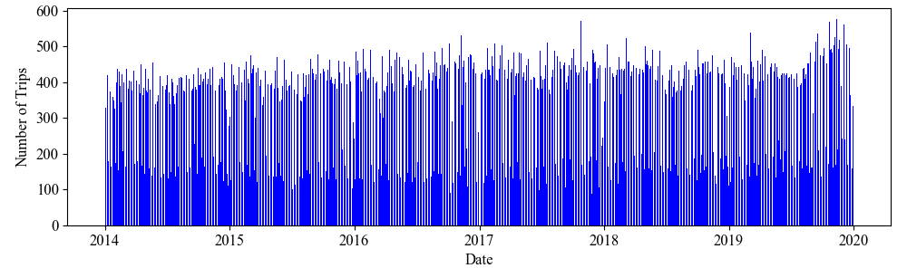
Figure 12: Daily Number of Trip Requests from January 2014 to December 2019.

Figure 12 indicates that weekdays experience a higher demand for trips compared to weekends and holidays. To ensure consistency in the demand pattern, the experiments exclusively utilize weekday trip request data. The training of the graph neural network described in Section 4 is conducted using data from workdays between January 2014 and November 2019. Data from December 2019 serves as the basis for evaluating performance.

Figure 13: Daily Number of Trip Requests in 2014.

For the purposes of this study, the number of drivers allocated each day is determined by the volume of trip requests for that day, calculated as follows:

$$n_{d}=\left\lceil\frac{n_{r}}{\omega}\right\rceil,$$ (11)

where $n_{d}$ denotes the number of drivers, $n_{r}$ represents the number of trip requests, and $\omega$ is the average number of trips a driver can manage in a day, which is set to 18 for this study.

5.2 Evaluation of the Graph Neural Network

This section presents the computational outcomes obtained by applying our proposed GNN models to the real-world dataset described in Section 5.1. The model training was conducted on a single Nvidia Tensor Core A100 80GB GPU, utilizing six nodes within a Linux environment on the PACE cluster (Partnership for an Advanced Computing Environment (2017), PACE). The implementation of the graph convolutional layers was carried out using version 2.4.0 of the PyTorch Geometric library. The loss function is minimized via gradient descent, using the Adam optimizer with weight decay as described in Kingma and Ba (2014). Additionally, it should be noted that each data point in the dataset correspond to a single graph. For graph-level mini-batching, the training follows the method outlined in PyTorch-Geometric (2023), where adjacency matrices for the same mini-batch are stacked diagonally, and the node-level features are concatenated along the node dimension.

Given the disparity between class distributions, with class 1 accounting for merely 8% of the labels, the evaluation metrics are carefully selected to reflect a balanced view of the model’s performance. In line with Morabit et al. (2023), the results utilize Recall, Specificity, and Balanced Accuracy as primary metrics.

Recall, AKA the true positive rate, assesses the model’s effectiveness in accurately identifying all instances of class 1. Specificity, AKA the true negative rate, evaluates how precisely the model detects negatives in the majority class. As the aim is to maximize both these metrics, Balanced Accuracy, i.e., the average of Recall and Specificity, is also included to offer a comprehensive metric reflecting the model’s overall accuracy for both classes.

The dataset excluding the test period spans from January 2014 to November 2019. The dataset is partitioned in an 80-20 split for training and validation sets. An adaptive learning strategy is applied to optimize the training. If the validation loss showed no improvement over several epochs, indicating a learning plateau, the learning rate is lowered to nudge the model towards better performance. In cases where this adjustment did not lead to any further gains, and to prevent the model from overfitting, early stopping is initiated. This step was crucial to retain the model’s ability to generalize to new data. The final set of configurations is given in Table 1.

Table 1: The Model Configurations After Tuning.

Hyperparameter	Value
Weight Decay	$5\times 10^{-6}$
$L_{1}$ Regularization Coeff. ($\lambda_{L_{1}}$)	$1\times 10^{-6}$
Class Weight Ratio ($w_{+}:w_{-}$)	$12:1$
Learning Rate	$3\times 10^{-4}$
Mini-batch Size	4
Number of Attention Heads	8
Hidden Dimensions	256
Dropout Rate	0.4
Res Gated GCN Layers	6

Figures 15 and 15 visually demonstrate the efficacy of the AGGNNI-CG’s learning capabilities through the training-validation loss curve and the Receiver Operating Characteristic (ROC) curve for the test set, respectively. In Figure 15, the initial steep decline in loss values across early epochs indicates rapid learning by the model. As training progresses, the loss curves for both datasets level off, signifying the model’s approach to a state with diminishing returns from further learning. This plateau is indicative not just of the model’s learning stabilization but also of the effectiveness of the early stopping mechanism which prevents overfitting.

The test set metrics for the GNN model are reported in Table 2. The learning model of AGGNNI-CG demonstrates a commendable level of accuracy in its predictions. With a recall of 91.5%, it accurately identifies most of the promising edges. Meanwhile, the specificity, standing at 85.4%, ensures that the high recall does not come at the cost of misclassifying the negative instances, thereby providing a comprehensive view of the model’s predictive performance. This means that the model’s selection of edges aligns closely with the expert choices.

The ROC curve, shown in Figure 15, corroborates these findings. With an AUC of 0.95, the curve articulates the model’s substantial discriminative power, signifying a high true positive rate at various threshold levels while maintaining a low false positive rate. This high AUC is particularly telling of the model’s proficiency in distinguishing between the two classes. The ROC curve’s proximity to the upper left corner signifies an almost ideal classifier, striking an effective balance between sensitivity and specificity. This is particularly notable given the challenge of maintaining high sensitivity in this highly unbalanced dataset without compromising specificity.

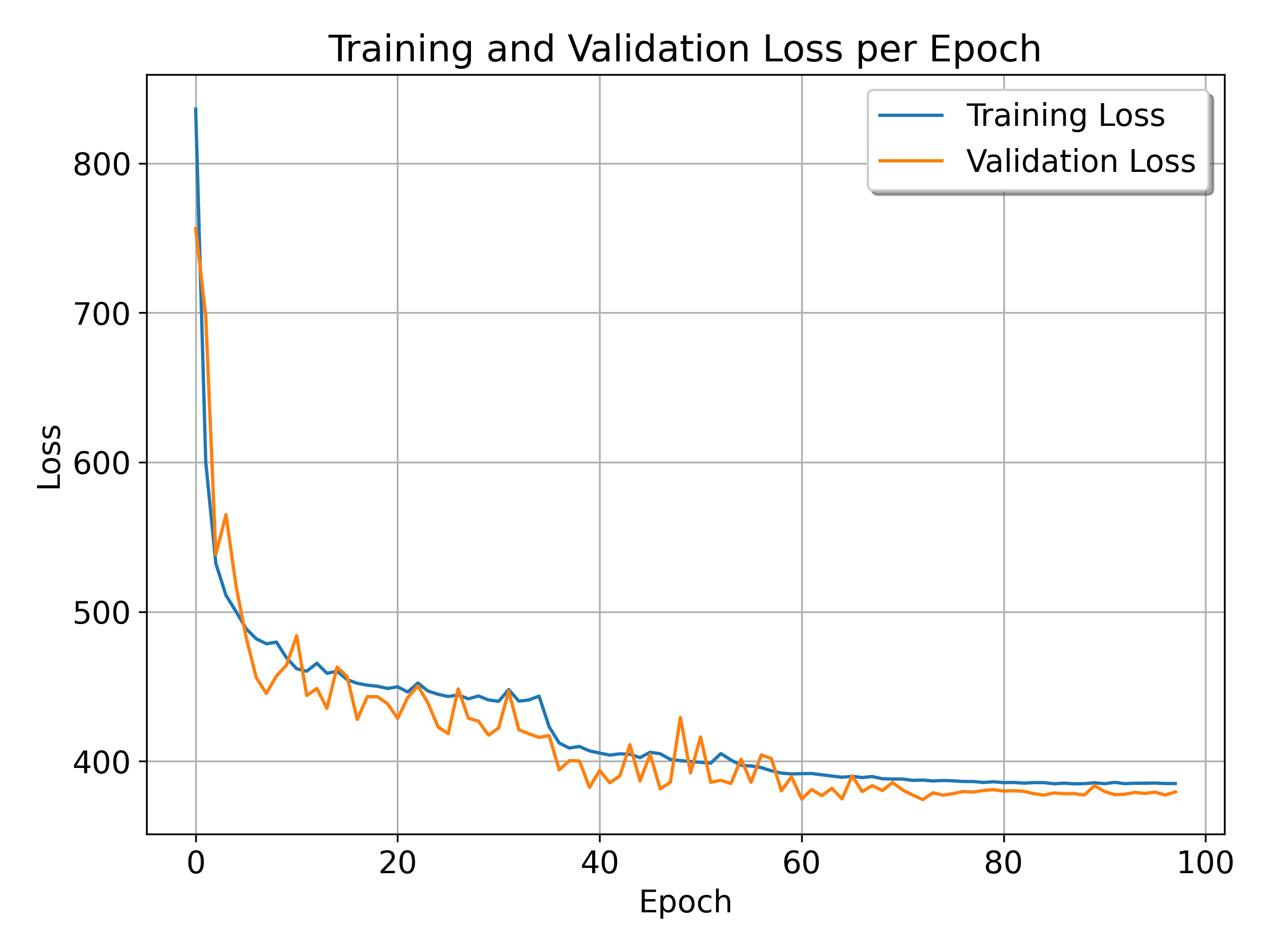
Figure 14: Train and validation loss per epoch

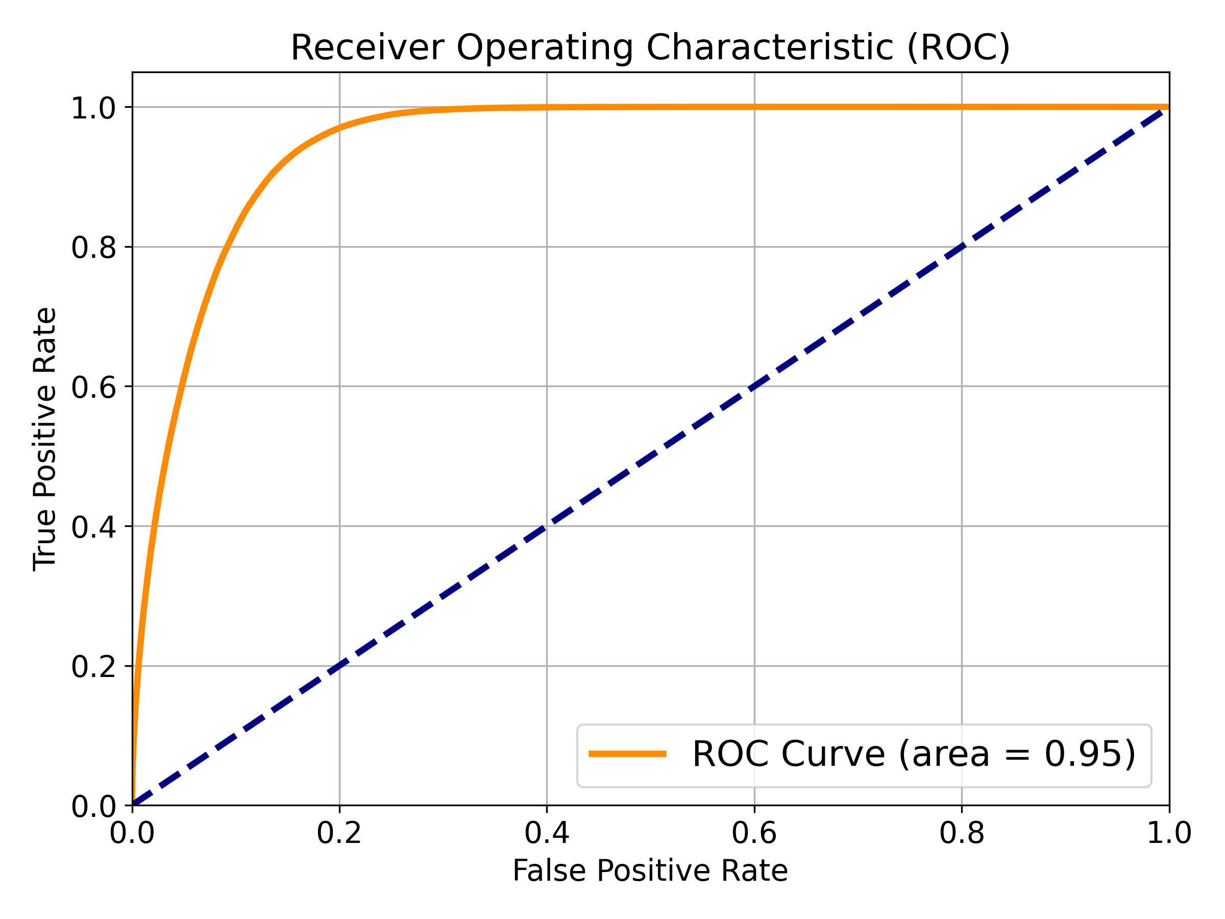
Figure 15: The ROC Curve for the Test Set.

Table 2: Accuracy Metrics for the Learning Step.

Metric	Value (%)
Recall	91.5
Specificity	85.4
Balanced Accuracy	88.5

5.3 Performance Analysis of the Column Generation

This section evaluates the performance differential between the conventional column generation approach (the baseline) and AGGNNI-CG. Consistent with the earlier discussion, the analysis is confined to weekday data to account for the stark contrasts in trip request patterns observed between weekdays and weekends. Additionally, data spanning December 23rd to December 31st is excluded from the evaluation set to mitigate the potential distortions arising from the Christmas holiday season. All evaluations were conducted on a 64-bit Linux server equipped with Dual Intel Xeon Gold 6226 CPUs at 2.7 GHz and 288 GB of RAM. Each instance was subject to a solution time limit set to 24 hours. If an instance cannot be solved within the time limit, its corresponding metrics are marked as ”-”.

To facilitate a more nuanced understanding of each method’s capabilities, this section first analyzes performance using instances with half of the trip requests. Table 3 presents the results of this analysis. In these reduced-demand scenarios, AGGNNI-CG almost always improves solution quality and produces order of magnitude improvements in efficiency. It also always finds a feasible solution contrary to the baseline. This trend is evident across most instances, highlighting the efficiency and effectiveness of AGGNNI-CG, even for instances of reduced complexity.

Table 3: Performance Comparison between the Baseline and AGGNNI-CG with half of the trip requests.

instance	baseline		AGGNNI-CG
	objective value	time (s)	objective value	time (s)
20191202	233	6,652	230	1,227
20191203	217	1,718	210	1,230
20191204	274	26,061	241	1,140
20191205	-	-	239	33,757
20191206	243	4,207	239	1,474
20191209	-	-	234	33,948
20191210	245	1,501	241	545
20191211	268	2,611	254	1,145
20191212	236	10,283	238	11,807
20191213	246	16,324	225	2,549
20191216	-	-	218	7,592
20191217	218	20,350	214	27,612
20191218	-	-	226	21,954
20191219	-	-	249	28,375
20191220	241	1,452	241	515

In the following, experiments on full trip requests are further evaluated. Table 4 explains the efficiency of AGGNNI-CG by providing a comparative overview of the original and reduced graphs for each test instance. The original graph for an instance is constructed by linking each node pair that satisfies the time window constraints, with nodes representing the pick-up and drop-off points of riders’ requests. This results in highly dense, all-to-all connectivity within the original graphs. Conversely, the reduced graph for each instance represents the output from the trained GNN, using the corresponding original graph as input. The “original graph” and “reduced graph” columns in Table 4 denote the number of edges present in each graph type per test instance. Remarkably, the implementation of the proposed GNN culminates in the elimination of approximately 94.9% of the edges from the original graphs. This pruning process retains a mere 5% of the edges, identified as “promising”, thereby drastically diminishing the size of the original graphs. Such substantial graph reduction explains the dramatuc speedups of AGGNNI-CG compared to the baseline.

Table 4: Number of edges in the original and reduced graphs.

instance	original graph	reduced graph	reduction (%)
20191202	902,025	47,624	94.7
20191203	853,314	46,439	94.6
20191204	1,258,323	38,513	96.9
20191205	1,060,385	53,847	94.9
20191206	1,035,815	49,401	95.2
20191209	971,703	46,307	95.2
20191210	1,031,748	39,853	96.1
20191211	1,205,055	39,264	96.7
20191212	1,023,638	48,317	95.3
20191213	1,043,973	46,525	95.5
20191216	913,458	44,505	95.1
20191217	831,288	42,048	94.9
20191218	898,230	45,108	95.0
20191219	1,072,778	48,350	95.5
20191220	987,539	47,335	95.2
average			94.9

Table 5 presents a comparative analysis of the baseline and AGGNNI-CG on the full instances. The baseline is only able to produce a solution for a single instance, highlighting its limitations. In stark contrast, the proposed method successfully generated high-quality solutions for all instances within a reasonable timeframe. For instance 20191203, the sole instance solved by the baseline, the objective value and computation time were recorded at 451 and 5,146 seconds, respectively. AGGNNI-CG, on the other hand, not only improved the objective value to 455 but also significantly reduced the computation time to 2,196 seconds. The computation times remain reasonable for AGGNNI-CG on all the other instances. This stark difference underscores the enhanced capability of AGGNNI-CG in addressing complex, real-world service scheduling challenges that are beyond the reach of traditional column generation algorithms. Additionally, the second column of Table 5 details both the total number of trip requests and the quantity successfully fulfilled by the current Paratransit system for each instance. On average, the existing Paratransit system manages to accommodate 80.91% of trip requests. In comparison, our proposed method shows a marked improvement, capable of servicing 91.15% of requests. This significant increase in efficiency underscores the practical advantages of implementing the proposed method in real-world settings.

A noteworthy observation from Table 5 is the extended computation time for instances 20191204 and 20191217. These instances, which have the highest and lowest numbers of trip requests, respectively, exhibit unique request patterns diverging from the norm. This variance potentially complicates the GNN predictions. Future enhancements could involve training the GNN model with more granularity in trip demand, aiming at refining the accuracy of edge prediction in varying demand scenarios.

Table 5: Performance Comparison between the Baseline and AGGNNI-CG on the Full Dataset

instance	total number of trip requests	baseline		AGGNNI-CG
	/ current system	objective value	time (s)	objective value	time (s)
20191202	474/365	-	-	438	8,192
20191203	461/342	451	5146	455	2,196
20191204	560/450	-	-	453	10,370
20191205	514/409	-	-	488	7,123
20191206	508/391	-	-	457	4,462
20191209	492/427	-	-	431	2,429
20191210	507/419	-	-	442	4,349
20191211	548/443	-	-	463	6,906
20191212	505/421	-	-	475	5,577
20191213	510/398	-	-	460	6,812
20191216	477/405	-	-	443	3,351
20191217	455/405	-	-	435	14,343
20191218	473/384	-	-	438	2,062
20191219	517/443	-	-	478	3,701
20191220	496/363	-	-	463	2,651

6 Conclusions

This study introduces AGGNNI-CG, an hybridization of machine learning and column generation designed to optimize service scheduling within Mobility as a Service (MaaS) frameworks. Central to this methodology is a graph neural network (GNN) tasked with producing reduced graphs, thereby streamlining the pricing subproblems of the column generation. AGGNNI-CG was applied to a real-world on-demand travel system and demonstrated an ability to condense the graphs pertinent to pricing subproblems by an order of magnitude, leading to dramatic acceleration of the conventional column generation process. For complex instances where traditional column generation methods falter, AGGNNI-CG successfully delivers high-quality solutions within a practical timeframe.

There are two primary avenues for expanding upon this research. First, while this study leverages a reservation-based on-demand travel system for performance validation, it would be highly interesting to apply a similar approach to real-world multimodal transit systems. Second, the current study focuses on weekday data, a limitation imposed by the prerequisites of GNN training, suggests an opportunity for future work to embrace data augmentation strategies. By enriching the dataset with augmented weekend and holiday data, it may be possible to evaluate — and indeed, enhance — the applicability of the proposed method across a broader spectrum of service scenarios, including weekends and public holidays.

References

- Amberg et al. (2019) Amberg, B., Amberg, B., Kliewer, N., 2019. Robust efficiency in urban public transportation: Minimizing delay propagation in cost-efficient bus and driver schedules. Transportation Science 53, 89–112.
- Andrade-Michel et al. (2021) Andrade-Michel, A., Ríos-Solís, Y.A., Boyer, V., 2021. Vehicle and reliable driver scheduling for public bus transportation systems. Transportation Research Part B: Methodological 145, 290–301.
- Auad et al. (2021) Auad, R., Dalmeijer, K., Riley, C., Santanam, T., Trasatti, A., Van Hentenryck, P., Zhang, H., 2021. Resiliency of on-demand multimodal transit systems during a pandemic. Transportation Research Part C: Emerging Technologies 133, 103418.
- Bengio et al. (2021) Bengio, Y., Lodi, A., Prouvost, A., 2021. Machine learning for combinatorial optimization: a methodological tour d’horizon. European Journal of Operational Research 290, 405–421.
- Borndörfer et al. (2017) Borndörfer, R., Schulz, C., Seidl, S., Weider, S., 2017. Integration of duty scheduling and rostering to increase driver satisfaction. Public Transport 9, 177–191.
- Braekers et al. (2014) Braekers, K., Caris, A., Janssens, G.K., 2014. Exact and meta-heuristic approach for a general heterogeneous dial-a-ride problem with multiple depots. Transportation Research Part B: Methodological 67, 166–186.
- Bresson and Laurent (2017) Bresson, X., Laurent, T., 2017. Residual gated graph convnets. arXiv preprint arXiv:1711.07553.
- Brody et al. (2021) Brody, S., Alon, U., Yahav, E., 2021. How attentive are graph attention networks? arXiv preprint arXiv:2105.14491.
- Cordeau (2006) Cordeau, J.F., 2006. A branch-and-cut algorithm for the dial-a-ride problem. Operations Research 54, 573–586.
- Cordeau and Laporte (2003) Cordeau, J.F., Laporte, G., 2003. A tabu search heuristic for the static multi-vehicle dial-a-ride problem. Transportation Research Part B: Methodological 37, 579–594.
- Cordeau and Laporte (2007) Cordeau, J.F., Laporte, G., 2007. The dial-a-ride problem: models and algorithms. Annals of operations research 153, 29–46.
- Cubillos et al. (2009) Cubillos, C., Urra, E., Rodríguez, N., 2009. Application of genetic algorithms for the darptw problem. International Journal of Computers Communications & Control 4, 127–136.
- Garaix et al. (2010) Garaix, T., Artigues, C., Feillet, D., Josselin, D., 2010. Vehicle routing problems with alternative paths: An application to on-demand transportation. European Journal of Operational Research 204, 62–75.
- Garaix et al. (2011) Garaix, T., Artigues, C., Feillet, D., Josselin, D., 2011. Optimization of occupancy rate in dial-a-ride problems via linear fractional column generation. Computers & Operations Research 38, 1435–1442.
- Goodall et al. (2017) Goodall, W., Dovey, T., Bornstein, J., Bonthron, B., 2017. The rise of mobility as a service. Deloitte Rev 20, 112–129.
- Gschwind and Drexl (2019) Gschwind, T., Drexl, M., 2019. Adaptive large neighborhood search with a constant-time feasibility test for the dial-a-ride problem. Transportation Science 53, 480–491.
- Gschwind and Irnich (2015) Gschwind, T., Irnich, S., 2015. Effective handling of dynamic time windows and its application to solving the dial-a-ride problem. Transportation Science 49, 335–354.
- Ho et al. (2018) Ho, S.C., Szeto, W.Y., Kuo, Y.H., Leung, J.M., Petering, M., Tou, T.W., 2018. A survey of dial-a-ride problems: Literature review and recent developments. Transportation Research Part B: Methodological 111, 395–421.
- Jain and Hentenryck (2011) Jain, S., Hentenryck, P.V., 2011. Large neighborhood search for dial-a-ride problems, in: Lee, J.H. (Ed.), Principles and Practice of Constraint Programming - CP 2011 - 17th International Conference, CP 2011, Perugia, Italy, September 12-16, 2011. Proceedings, Springer. 400–413. 10.1007/978-3-642-23786-7\_31.
- Jorgensen et al. (2007) Jorgensen, R.M., Larsen, J., Bergvinsdottir, K.B., 2007. Solving the dial-a-ride problem using genetic algorithms. Journal of the operational research society 58, 1321–1331.
- Joshi et al. (2019) Joshi, C.K., Laurent, T., Bresson, X., 2019. An efficient graph convolutional network technique for the travelling salesman problem. arXiv preprint arXiv:1906.01227.
- Kang et al. (2019) Kang, L., Chen, S., Meng, Q., 2019. Bus and driver scheduling with mealtime windows for a single public bus route. Transportation Research Part C: Emerging Technologies 101, 145–160.
- Karimi-Mamaghan et al. (2022) Karimi-Mamaghan, M., Mohammadi, M., Meyer, P., Karimi-Mamaghan, A.M., Talbi, E.G., 2022. Machine learning at the service of meta-heuristics for solving combinatorial optimization problems: A state-of-the-art. European Journal of Operational Research 296, 393–422.
- Kingma and Ba (2014) Kingma, D.P., Ba, J., 2014. Adam: A method for stochastic optimization. arXiv preprint arXiv:1412.6980.
- Kipf and Welling (2016) Kipf, T.N., Welling, M., 2016. Semi-supervised classification with graph convolutional networks. arXiv preprint arXiv:1609.02907.
- Kirchler and Calvo (2013) Kirchler, D., Calvo, R.W., 2013. A granular tabu search algorithm for the dial-a-ride problem. Transportation Research Part B: Methodological 56, 120–135.
- Lu et al. (2022) Lu, J., Nie, Q., Mahmoudi, M., Ou, J., Li, C., Zhou, X.S., 2022. Rich arc routing problem in city logistics: Models and solution algorithms using a fluid queue-based time-dependent travel time representation. Transportation Research Part B: Methodological 166, 143–182.
- Mazyavkina et al. (2021) Mazyavkina, N., Sviridov, S., Ivanov, S., Burnaev, E., 2021. Reinforcement learning for combinatorial optimization: A survey. Computers & Operations Research 134, 105400.
- Mladenovic (2021) Mladenovic, M., 2021. Mobility as a service, in: International Encyclopedia of Transportation. Elsevier.
- Morabit et al. (2021) Morabit, M., Desaulniers, G., Lodi, A., 2021. Machine-learning–based column selection for column generation. Transportation Science 55, 815–831.
- Morabit et al. (2023) Morabit, M., Desaulniers, G., Lodi, A., 2023. Machine-learning–based arc selection for constrained shortest path problems in column generation. INFORMS Journal on Optimization 5, 191–210.
- Nazari et al. (2018) Nazari, M., Oroojlooy, A., Snyder, L., Takác, M., 2018. Reinforcement learning for solving the vehicle routing problem. Advances in neural information processing systems 31.
- Partnership for an Advanced Computing Environment (2017) (PACE) Partnership for an Advanced Computing Environment (PACE), 2017. PACE - Partnership for an Advanced Computing Environment. [Online; accessed 18-December-2023].
- Portugal et al. (2009) Portugal, R., Lourenço, H.R., Paixão, J.P., 2009. Driver scheduling problem modelling. Public Transport 1, 103–120.
- PyTorch-Geometric (2023) PyTorch-Geometric, 2023. Batching — pytorch geometric 2023 documentation. https://pytorch-geometric.readthedocs.io/en/latest/advanced/batching.html. Accessed: 2023-12-26.
- Qu and Bard (2015) Qu, Y., Bard, J.F., 2015. A branch-and-price-and-cut algorithm for heterogeneous pickup and delivery problems with configurable vehicle capacity. Transportation Science 49, 254–270.
- Riley et al. (2019) Riley, C., Legrain, A., Van Hentenryck, P., 2019. Column generation for real-time ride-sharing operations, in: Integration of Constraint Programming, Artificial Intelligence, and Operations Research: 16th International Conference, CPAIOR 2019, Thessaloniki, Greece, June 4–7, 2019, Proceedings 16, Springer. 472–487.
- Ropke et al. (2007) Ropke, S., Cordeau, J.F., Laporte, G., 2007. Models and branch-and-cut algorithms for pickup and delivery problems with time windows. Networks: An International Journal 49, 258–272.
- Ropke and Pisinger (2006) Ropke, S., Pisinger, D., 2006. An adaptive large neighborhood search heuristic for the pickup and delivery problem with time windows. Transportation science 40, 455–472.
- Shen et al. (2022) Shen, Y., Sun, Y., Li, X., Eberhard, A., Ernst, A., 2022. Enhancing column generation by a machine-learning-based pricing heuristic for graph coloring, in: Proceedings of the AAAI Conference on Artificial Intelligence, 9926–9934.
- Smith (2020) Smith, G., 2020. Making mobility-as-a-service: Towards governance principles and pathways. Ph.D. thesis. Chalmers Tekniska Hogskola (Sweden).
- Smith et al. (2018) Smith, G., Sochor, J., Sarasini, S., 2018. Mobility as a service: Comparing developments in sweden and finland. Research in Transportation Business & Management 27, 36–45.
- Tóth and Krész (2013) Tóth, A., Krész, M., 2013. An efficient solution approach for real-world driver scheduling problems in urban bus transportation. Central European Journal of Operations Research 21, 75–94.
- Van Hentenryck et al. (2023) Van Hentenryck, P., Riley, C., Trasatti, A., Guan, H., Santanam, T., Huertas, J.A., Dalmeijer, K., Watkins, K., Drake, J., Baskin, S., 2023. Marta reach: Piloting an on-demand multimodal transit system in atlanta. arXiv preprint arXiv:2308.02681.
- Veličković et al. (2017) Veličković, P., Cucurull, G., Casanova, A., Romero, A., Lio, P., Bengio, Y., 2017. Graph attention networks. arXiv preprint arXiv:1710.10903.
- Vinyals et al. (2015) Vinyals, O., Fortunato, M., Jaitly, N., 2015. Pointer networks. Advances in neural information processing systems 28.
- Wren and Wren (1995) Wren, A., Wren, D.O., 1995. A genetic algorithm for public transport driver scheduling. Computers & Operations Research 22, 101–110.
- Yuan et al. (2022a) Yuan, E., Chen, W., Hentenryck, P.V., 2022a. Reinforcement learning from optimization proxy for ride-hailing vehicle relocation. J. Artif. Intell. Res. 75, 985–1002. 10.1613/JAIR.1.13794.
- Yuan et al. (2022b) Yuan, H., Jiang, P., Song, S., 2022b. The neural-prediction based acceleration algorithm of column generation for graph-based set covering problems, in: 2022 IEEE International Conference on Systems, Man, and Cybernetics (SMC), IEEE. 1115–1120.