Active nematics that modify their environment: a framework for extra-cellular matrix remodeling

Abstract

Many exemplary active systems, including living cells and animals, are able to form nematic order, while interacting with their environment. In this Letter, we explain how a dynamic coupling of an active nematic with its environment results in novel physical behavior. Deposition of aligned environment segments modifies the isotropic-nematic phase diagram and allows for nematic order at arbitrarily low densities. The aligned environment acts as an external field that may also lead to arrested angular dynamics. We are motivated mainly by cells that remodel collagen fibers in the extra-cellular matrix (ECM), while being guided by the fibers during multicellular migration. Our predictions indicate that remodeling promotes macroscopic cellular order and ECM patterning, and possibly limits the coarsening of ordered ECM domains, in accordance with recent experiments.

Active nematics are systems composed of self-propelling constituents that can form a nematic (apolar) orientational order. Orientational order has far-reaching consequences in active systems due to its coupling with propulsion, which leads to macroscopic currents Ramaswamy (2010); Marchetti et al. (2013); Chaté (2020). This has motivated many physical studies of the active isotropic-nematic transition Chaté (2020); Peshkov et al. (2012); Ngo et al. (2014); Großmann et al. (2016). Similar to passive liquid crystals, order is driven by strong aligning fields, obtained by a combination of strong interactions (low ”temperature”) and high densities. Active propulsion then leads to possible coexistence between a dilute isotropic phase and dense nematic phase.

Active nematics are ubiquitous in biological systems at different scales. Our main motivation is cells in extra-cellular matrix (ECM). Both cells and collagen fibers in ECM can exhibit nematic order. Growing evidence suggests that the interplay between cellular and ECM order is essential for tissue patterning and multicellular migration Clark and Vignjevic (2015); Alexander and Cukierman (2016); Helvert et al. (2018); Wershof et al. (2019); Park et al. (2020). In particular, aligned collagen structures have been shown to greatly promote metastasis Conklin et al. (2011); Kopanska et al. (2016). However, the macrosocpic physical mechanisms underlying cell-ECM interplay and its role in cell and ECM order and dynamics are not well understood.

Our approach to understand cell-ECM interplay is to consider them as a two-component active system. We recently applied such a framework to explain mechanical feedback mechanisms between cells and ECM Adar and Joanny (2021, 2022). Here we focus on chemical ECM remodeling, including deposition, degradation, and alignment by active cells. This is done in-vivo mainly by fibroblast cells Phillips et al. (2009); Sahai et al. (2020). We find that ECM allows for steady-state nematic order at arbitrarily low cellular densities, which is linearly stable. In the ordered phase, ECM acts as an external field that may pin the cells and constrain their angular relaxation. While we are motivated by cells in ECM, our theory should serve as basis for the study of general active matter that interacts with a dynamic environment.

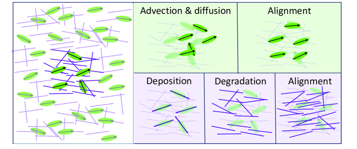
Figure 1: (Color online) Heuristic description of cell-matrix model and possible dynamics. Cells are illustrated as green ellipses and their orientation is indicated with a black arrow. ECM segments are illustrated as purple lines. Left: focus on a small region in space. Top bars (green background): cells can either advect and diffuse or align with other cells and fibers. Bottom bars (purple background) segments can either be deposited, degraded or aligned by cells.

Theory. We consider active cells and passive matrix segments in two dimensions, each described by their position and orientation, $\boldsymbol{r}$ and $\boldsymbol{n}$ for the cells and $\boldsymbol{r}^{\prime}$ and $\boldsymbol{n}^{\prime}$ for the matrix. Cells self-propel with a velocity $\boldsymbol{v}=v\boldsymbol{n}$ and diffuse with a diffusion coefficient $D$. In addition, they align with neighboring cells and matrix segments. Matrix segments are considered to be apolar. They are enslaved to the cells that may deposit segments, degrade them or re-arrange them (see Fig. 1). These dynamics are described by the following equations:

$$\frac{\partial f_{\mathrm{c}}}{\partial t} =-\nabla\cdot\left(f_{\mathrm{c}}v\boldsymbol{n}\right)+D\nabla^{2}f_{\mathrm{c}}-kf_{\mathrm{c}}+k\rho_{\mathrm{c}}\frac{\mathrm{e}^{-E_{\mathrm{c}}}}{Z_{\mathrm{c}}}$$

$$\frac{\partial f_{\mathrm{m}}}{\partial t} =\frac{k_{+}}{2}\left[f_{\mathrm{c}}\left(\boldsymbol{r}^{\prime},\boldsymbol{n}^{\prime}\right)+f_{\mathrm{c}}\left(\boldsymbol{r}^{\prime},-\boldsymbol{n}^{\prime}\right)\right]-k_{-}\rho_{\mathrm{c}}f_{\mathrm{m}}$$

$$-k_{0}f_{\mathrm{m}}+k_{0}\rho_{\mathrm{m}}\frac{\mathrm{e}^{-E_{\mathrm{m}}}}{Z_{\mathrm{m}}}.$$ (1)

The function $f_{\mathrm{c}}$ ($f_{\mathrm{m}}$) describes the distribution to find a cell (matrix segment) at position $\boldsymbol{r}$ ($\boldsymbol{r}^{\prime}$) with orientation $\boldsymbol{n}$ ($\boldsymbol{n}^{\prime}$). They are normalized such that $\int\mathrm{d}\boldsymbol{n}f_{\mathrm{c}}=\rho_{\mathrm{c}}$ is the cellular density and $\int\mathrm{d}\boldsymbol{n}^{\prime}f_{\mathrm{m}}=\rho_{\mathrm{m}}$ is the matrix density.

The cellular orientation dynamics are written in terms of the tumbling rate $k$, and an orientation probability, given by the Boltzmann factor $\exp\left(-E_{\mathrm{c}}\right)/Z_{\mathrm{c}}$ with the alignment energy $E_{\mathrm{c}}$ and partition function $Z_{\mathrm{c}}=\int\mathrm{d}\boldsymbol{n}\exp\left(-E_{\mathrm{c}}\right)$. This is a convenient choice that allows for the recovery of passive systems in simple limits. Matrix orientation dynamics are similarly described, given by the rate $k_{0}$ and the Boltzmann factor $\exp\left(-E_{\mathrm{m}}\right)/Z_{\mathrm{m}}$. Finally, matrix deposition and degradation are described by the rates $k_{+}\rho_{\mathrm{c}}$ and $k_{-}\rho_{\mathrm{c}}$, respectively. Here we assume that cells locally deposit segments along their axis of motion and degrade segments in all orientations.

Averaging the different moments of the orientation angles yield mesoscopic fields that are the focus of the hydrodynamic equations. The cellular current density is given by $\boldsymbol{j}=v\int\mathrm{d}\boldsymbol{n}f_{\mathrm{c}}$, the cellular nematic tensor density is $\boldsymbol{Q}_{\mathrm{c}}=\int\mathrm{d}\boldsymbol{n}\,\left(\boldsymbol{n}\boldsymbol{n}-\boldsymbol{I}/2\right)f_{\mathrm{c}}$, and the matrix nematic tensor density is $\boldsymbol{Q}_{\mathrm{m}}=\int\mathrm{d}\boldsymbol{n}^{\prime}\,\left(\boldsymbol{n}^{\prime}\boldsymbol{n}^{\prime}-\boldsymbol{I}/2\right)f_{\mathrm{m}}.$ These fields are all extensive in the number of cells/matrix segments.

We coarse-grain Eq. (Active nematics that modify their environment: a framework for extra-cellular matrix remodeling) into hydrodynamic equations in terms of the average fields. In particular, we treat the orientation within mean field (MF) in terms of the interactions $E_{\mathrm{c}}\left(\boldsymbol{n}\right)=-2\text{Tr}\left[\left(\boldsymbol{n}\boldsymbol{n}-\boldsymbol{I}/2\right)\boldsymbol{Q}_{t}\right]$ with $\boldsymbol{Q}_{t}=\beta_{\mathrm{c}}\boldsymbol{Q}_{\mathrm{c}}+\beta_{\mathrm{m}}\boldsymbol{Q}_{\mathrm{m}}$ and $E_{\mathrm{m}}\left(\boldsymbol{n}^{\prime}\right)=-2\text{Tr}\left[\left(\boldsymbol{n}^{\prime}\boldsymbol{n}^{\prime}-\boldsymbol{I}/2\right)\beta_{\mathrm{m}}\boldsymbol{Q}_{\mathrm{c}}\right]$. Here we assume that the cells align with neighboring cells and matrix segments according to the interaction strengths $\beta_{\mathrm{c}}$ and $\beta_{\mathrm{m}}$, respectively, while the matrix is only aligned by the cells. For more general choices, including non-reciprocal interactions, see SM in SMa . Note that the cells are effectively aligned by the total nematic tensor $\boldsymbol{Q}_{t}$ that includes cellular and matrix contributions. In the absence of cell activity and cell-matrix interaction, our choice of $E_{\mathrm{c}}$ leads to an equivalent of Maier-Saupe theory De Gennes and Prost (1993) for compressible systems.

The resulting hydrodynamic equations are SMa :

$$\frac{\partial\rho_{\mathrm{c}}}{\partial t} =D\nabla^{2}\rho_{\mathrm{c}}-\nabla\cdot\boldsymbol{j},$$

$$\frac{\partial\boldsymbol{j}}{\partial t} =D\nabla^{2}\boldsymbol{j}-\frac{v^{2}}{2}\nabla\rho_{\mathrm{c}}-v^{2}\nabla\cdot\boldsymbol{Q}_{\mathrm{c}}-k\boldsymbol{j},$$

$$\frac{\partial\boldsymbol{Q}_{\mathrm{c}}}{\partial t} =D\nabla^{2}\boldsymbol{Q}_{\mathrm{c}}-\frac{1}{4}\left(\nabla\boldsymbol{j}+\nabla\boldsymbol{j}^{\mathrm{T}}-\nabla\cdot\boldsymbol{j}\boldsymbol{I}\right)$$

$$-k\,\boldsymbol{Q}_{\mathrm{c}}+k\rho_{\mathrm{c}}\,g\left(Q_{t}\right)\frac{\boldsymbol{Q}_{t}}{Q_{t}},$$

$$\frac{\partial\rho_{\mathrm{m}}}{\partial t} =\rho_{\mathrm{c}}\left(k_{+}-k_{-}\rho_{\mathrm{m}}\right),$$

$$\frac{\partial\boldsymbol{Q}_{\mathrm{m}}}{\partial t} =k_{+}\boldsymbol{Q}_{\mathrm{c}}-k_{-}\rho_{\mathrm{c}}\boldsymbol{Q}_{\mathrm{m}}$$

$$-k_{0}\boldsymbol{Q}_{\mathrm{m}}+k_{0}\rho_{\mathrm{m}}\,g\left(\beta_{\mathrm{m}}Q_{\mathrm{c}}\right)\frac{\boldsymbol{Q}_{\mathrm{c}}}{Q_{\mathrm{c}}}.$$ (2)

The first equation is the cellular continuity equation, written in terms of the active cellular current $\boldsymbol{j}$ and a passive diffusive current. The second equation is a polarization-rate equation for the active current. At steady-state, it can be interpreted as a force balance equation (see below).

The equation for $\boldsymbol{Q}_{\mathrm{c}}$ includes diffusion and shear-alignment (first line), as well as non-linear alignment terms that dominate at large lengthscales. They are written in terms of the function $g(x)=I_{1}(x)/I_{0}(x),$ where $I_{n}(x)$ is the modified Bessel function of the first kind Abramowitz et al. (1988). $g(x)$ plays a similar role to $\tanh x$ in the standard MF treatment of the Ising model. The cellular dynamics include both the first and second moments of the angular distribution ($\boldsymbol{j}$ and $\boldsymbol{Q}_{\mathrm{c}}$, respectively), similarly to “self-propelled rods” Marchetti et al. (2013); Peruani et al. (2006); Baskaran and Marchetti (2008). Finally, the matrix dynamics are governed by cellular deposition and degradation, while $\boldsymbol{Q}_{\mathrm{m}}$ has an additional nonlinear alignment term $\sim k_{0}$. For simplicity, we focus on matrix deposition and degradation, and set $k_{0}=0$ hereafter.

These equations define our framework for active nematics (cells) that modify their environment (matrix), which we apply for the study of ECM remodeling. Cell-matrix interplay enters the theory in two ways: cellular alignment by the matrix as part of the nematic tensor $\boldsymbol{Q}_{t}$ and matrix remodeling by the cells. Cellular activity also enters our theory in several ways: the active current $\boldsymbol{j}$, the deposition and degradation of matrix segments, and possibly in the alignment dynamics.

Next, we focus on the consequences of remodeling on the emergence of cellular and ECM orientational order at steady state as well as typical relaxation dynamics of the cell and matrix. For brevity, we rescale times with $1/k$ and lengths with $v/k$, the typical cellular persistence length, while keeping the same notation.

Steady-state phase diagram. The standard isotropic-nematic transition in active systems is similar to a gas-liquid transition Chaté (2020); Solon and Tailleur (2013), where the alignment strength plays the role of inverse temperature. At low densities and high temperatures, the system forms a dilute isotropic gas, while at high densities and low temperatures - a nematic liquid. At intermediate densities and temperatures, the two phases co-exist and are generally linearly unstable. Here, using a MF theory, we show how the matrix can break this behavior, by allowing nematic order at arbitrarily low cellular densities.

The key to understand the coexistence lies in the stress. In the hydrodynamic limit of large system size and long time, the steady-state behavior of the cells can be described by a constant stress tensor SMa , $\boldsymbol{\sigma}=-\left[\boldsymbol{I}+2\boldsymbol{Q}_{\mathrm{c}}/\left(1+2D\right)\right]$. We consider a possible density profile along the $x$ direction and focus on the $xx$ component of the stress that we denote as $\sigma$ for brevity,

$$\sigma=\sigma_{xx}=-\left(\rho_{\mathrm{c}}+\frac{Q_{\mathrm{c}}}{1+2D}\right).$$ (3)

The first term is the ideal-gas contribution to the pressure, while the second term is an extensile active stress $\sim\boldsymbol{Q}_{\mathrm{c}}$. Here we assume that order forms either along the $x$ axis ($Q_{\mathrm{c}}>0$) or the $y$ axis ($Q_{\mathrm{c}}<0$).

Co-existence is possible when the active stress decreases with density, compensating for the increase in ideal-gas pressure. This is the scenario when cells align in the $y$ direction. The stress $\sigma$ can be considered as a Lagrange multiplier that enforces the total number of cells. It is given by the density in the isotropic phase.

Next, we derive the isostropic-nematic phase diagram in the density-temperature plane, where $\beta_{\mathrm{c}},\beta_{\mathrm{m}}\sim 1/T$. Examples of such phase diagrams with and without a matrix (ECM) are given in Figs. 2a and Figs. 2b. The region of co-existence is delimited by the binodal line (solid blue line), within which lies a region of linear instability, delimited by the spinodal line (dashed red line).

As the phase diagram is derived around steady state, the matrix density and nematic order are given by the steady-state solutions to Eq. (Active nematics that modify their environment: a framework for extra-cellular matrix remodeling). The matrix density is $\rho_{\mathrm{m}}=k_{+}/k_{-}$, independent of $\rho_{\mathrm{c}}$. This is important because at long times, even an arbitrarily dilute collection of cells deposits a finite-density matrix, which can serve as an external field for its alignment.

The matrix nematic tensor forms along the same axis as the cellular order. The system is invariant to this choice of axis, and we focus here on the magnitude of nematic order, $Q_{\mathrm{m}}$. We define the intensive nematic order of the cells and matrix, $q_{\mathrm{c}}=Q_{\mathrm{c}}/\rho_{\mathrm{c}}$ and $q_{\mathrm{m}}=Q_{\mathrm{m}}/\rho_{\mathrm{m}}$, and find that

$$q_{\mathrm{m}}=q_{\mathrm{c}}.$$ (4)

The matrix inherits the same intensive nematic order as the cells. The matrix contribution to $Q_{t}$ dominates at low cellular concentration and allows for matrix-driven alignment among dilute cells.

Next, we analyze the effect of ECM remodeling on the spinodal and binodal lines, as is plotted in Fig. 2.

Spinodal. The spinodal is given by $\partial\sigma/\partial\rho_{\mathrm{c}}=0$ for fixed values of $\beta_{\mathrm{c}}$ and $\beta_{\mathrm{m}}$. This threshold of linear instability is due to a negative compressibility; As the cellular density increases, the active stress overcomes the osmotic pressure and pushes cells up their concentration gradient. Note that active nematics can also be unstable due to a combination of active stress and shear alignment Voituriez et al. (2005); Duclos et al. (2018), but this is not the case here, where the cells are effectively extensile and align with the strain rate.

Negative compressibility occurs for $\partial Q_{\mathrm{c}}/\partial\rho_{\mathrm{c}}<-\left(1+2D\right)$ [Eq. (3)]. In the isotropic state, $Q_{\mathrm{c}}\equiv 0$ and this is not possible. Deep in the ordered state, $Q_{\mathrm{c}}=\pm\rho_{\mathrm{c}}$, also ensuring stability. The instability is possible, therefore, only for intermediate $Q_{\mathrm{c}}$ values. For such values we expand the nonlinear terms of the $Q_{\mathrm{c}}$ equation in Eq. (Active nematics that modify their environment: a framework for extra-cellular matrix remodeling) and find its possible roots. One solution is $Q_{\mathrm{c}}=0$ and the other is $Q_{\mathrm{c}}=-\rho_{\mathrm{c}}\sqrt{\left(\beta_{\mathrm{m}}\rho_{\mathrm{m}}+\beta_{\mathrm{c}}\rho_{\mathrm{c}}-2\right)/\left(\beta_{\mathrm{m}}\rho_{\mathrm{m}}+\beta_{\mathrm{c}}\rho_{\mathrm{c}}\right)^{3}},$ such that $q_{\mathrm{c}}$ depends only on $\beta_{\mathrm{m}}\rho_{\mathrm{m}}+\beta_{\mathrm{c}}\rho_{\mathrm{c}}$.

First, we examine the case of $\beta_{\mathrm{m}}\rho_{\mathrm{m}}<2.$ The cells are isotropic at low densities and become ordered at $\rho_{\ast}=\left(2-\beta_{\mathrm{m}}\rho_{\mathrm{m}}\right)/\beta_{\mathrm{c}}$. As $Q_{\mathrm{c}}\sim\sqrt{\rho-\rho_{\ast}}$ in this case, $\partial Q_{\mathrm{c}}/\partial\rho_{\mathrm{c}}\ll-1$ and the system is unstable. $\rho_{\ast}$ thus marks the gas spinodal line. Otherwise, for $\beta_{\mathrm{m}}\rho_{\mathrm{m}}>2,$ the cells can be ordered even at vanishing densities (see gray region in Fig. 2b). This is the main effect of the matrix. The slope $\partial Q_{\mathrm{c}}/\partial\rho_{\mathrm{c}}$ at vanishing densities is then given by $\sqrt{\left(\beta_{\mathrm{m}}\rho_{\mathrm{m}}-2\right)/\left(\beta_{\mathrm{m}}\rho_{\mathrm{m}}\right)^{3/2}}$. As this quantity is always smaller than unity, the system is stable.

Binodal. The binodal describes, for a given temperature, the densities of the macroscopic phases at coexistence. We find it by focusing on the equation for $Q_{\mathrm{c}},$ while replacing $\rho_{\mathrm{c}}$ by its value at steady state, $\rho_{\mathrm{c}}=-\sigma-Q_{\mathrm{c}}/\left(1+2D\right)$. Upon proper rescaling of lengths SMa , we find that

$$Q_{\mathrm{c}}^{\prime\prime}=Q_{\mathrm{c}}+\left(\sigma+\frac{Q_{\mathrm{c}}}{1+2D}\right)g\left(Q_{t}\right)\equiv F\left(\sigma,Q_{\mathrm{c}}\right).$$ (5)

This has the same structure as Newton’s equation, where $Q_{\mathrm{c}}$ plays the role of position and the $x$ coordinate - the role of time, while $F$ is the force (see also Solon et al. (2015)). The first integral (conservation of energy) yields $E=Q_{\mathrm{c}}^{\prime 2}/2+U$, where we have denoted the potential energy $U=-\int\mathrm{d}Q_{\mathrm{c}}\,F\left(\sigma,Q_{\mathrm{c}}\right).$

Continuing the analogy to a Newtonian particle, the binodal requires two $Q_{\mathrm{c}}$ values that have the same energy, such that there is co-existence, and where the force vanishes, $F=0$, such that it takes an infinite time to escape them. These two conditions set $Q_{\mathrm{l}}$, the nematic order in the dense liquid phase, as well as $-\sigma=\rho_{\mathrm{g}}$, the density in the isotropic gas phase. To summarize, we require that $Q_{\mathrm{c}}=0,Q_{\mathrm{l}}$ are degenerate roots of $U$.

We highlight the effect of matrix remodeling by focusing on two limits: a cell-dominated interaction $U\left(\beta_{\mathrm{m}}=0\right)=U_{\mathrm{c}}$ where there is no matrix, and a matrix-dominated one $U\left(\beta_{\mathrm{c}}=0\right)=U_{\mathrm{m}}$, where the cells are aligned only by the matrix. Explicitly,

$$U_{\mathrm{c}}\left(Q_{\mathrm{c}}\right) =\int_{0}^{Q_{\mathrm{c}}}\mathrm{d}Q\left[\rho_{\mathrm{c}}(Q)g\left(\beta_{\mathrm{c}}Q\right)-Q\right],$$

$$U_{\mathrm{m}}\left(Q_{\mathrm{c}}\right) =\int_{0}^{Q_{\mathrm{c}}}\mathrm{d}Q\left[\rho_{\mathrm{c}}(Q)g\left(\tilde{\beta_{\mathrm{m}}}q_{\mathrm{c}}(Q)\right)-Q\right],$$ (6)

where $\tilde{\beta_{\mathrm{m}}}=\rho_{\mathrm{m}}\beta_{\mathrm{m}}.$ The difference between the two cases is the magnitude of the total nematic tensor ($Q_{t}$), which appears as the argument of the nonlinear $g$ function. In the cell-dominated case, the argument scales as the extensive $Q_{\mathrm{c}}$ that vanishes at small densities, while the matrix-dominated cases - as the intensive $q_{\mathrm{c}}$. The two potentials are plotted in Fig. 2c.

The cell-dominated potential has an important property. Multiplying it by $\beta_{\mathrm{c}}^{2}$, we find that it depends only on $\beta_{\mathrm{c}}\rho_{\mathrm{c}}$ and $\beta_{\mathrm{c}}Q$. This means that both the spinodal and binodal are given by straight lines $\beta_{\mathrm{c}}\rho_{\mathrm{c}}=\mathrm{const,}$ as is evident from Fig. 2a. In particular, we find that the nematic order at the liquid binodal $\beta_{\mathrm{c}}Q_{\mathrm{l}}$ is not necessarily small SMa . Therefore, we cannot find it from an expansion of $U_{\mathrm{c}}$, but rather from its full nonlinear form. Our numerical calculations show that there is indeed a coexistence between an isotropic gas and nematic liquid. This is obtained from the maxima of $U_{\mathrm{c}}$ and from numerical solutions of Eq. (Active nematics that modify their environment: a framework for extra-cellular matrix remodeling), plotted in Figs. 2c and 2d. We find $\rho_{\mathrm{g}}$ numerically, and $\rho_{\mathrm{l}}$ is then found by requiring a fixed stress, i.e., $\rho_{\mathrm{g}}=\rho_{\mathrm{l}}+Q_{\mathrm{l}}/\left(1+2D\right)$.

The situation is very different in the matrix-dominated case. We expand for small $Q_{\mathrm{c}}$ and find $U_{\mathrm{m}}\sim-Q_{\mathrm{c}}^{2}\left[Q_{\mathrm{c}}^{2}-16\sigma^{2}\tilde{\beta_{\mathrm{m}}}^{-3}\left(-2+\tilde{\beta_{\mathrm{m}}}\right)\right]$. In this case, $Q_{\mathrm{c}}=0$ is a local minimum and the global maxima are $Q_{\mathrm{c}}=\pm 2\sigma\sqrt{\tilde{\beta_{\mathrm{m}}}^{-3}\left(-2+\tilde{\beta_{\mathrm{m}}}\right)}$. The value of $q_{\mathrm{c}}$ in this case depends only on $\tilde{\beta_{\mathrm{m}}}$. This is clear from the steady-state condition $q_{\mathrm{c}}=g\left(\tilde{\beta_{\mathrm{m}}}q_{\mathrm{c}}\right)$.

The potential $U_{\mathrm{m}}\left(\tilde{\beta_{\mathrm{m}}}>2\right)$ infers co-existence of nematic order along the $x$ and $y$ directions for any density. This is obtained from the maxima of $U_{\mathrm{m}}$ and from numerical solutions of Eq. (Active nematics that modify their environment: a framework for extra-cellular matrix remodeling), plotted in Figs. 2c and 2e. This new type of coexistence is possible because cells order at arbitrarily low densities. Then, cells aligned along the $x$ direction at very low densities can exert a positive active stress that matches $\sigma$. Note that as $\tilde{\beta_{\mathrm{m}}}$ becomes larger, the potential becomes less symmetric and its global maximum is for negative $Q_{\mathrm{c}}$ values (see Fig. 2c). Positive values of $Q_{\mathrm{c}}$ and co-existence then become transient.

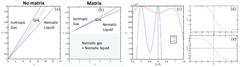
Figure 2: (Color online) (a+b) Phase diagrams in the density and temperature plane (a) without a matrix and (b) with a matrix. We consider $\rho=\rho_{\mathrm{c}}$ and $T=1/\beta_{\mathrm{c}}$. Solid blue lines are the binodal and dahsed red ones are the spinodal. The values used are: $D=0.5$, $\beta_{\mathrm{m}},\rho_{\mathrm{m}}=0$ (a) and $D=0.5$, $\beta_{\mathrm{m}}=\beta_{\mathrm{c}},\rho_{\mathrm{m}}=5$ (b).(c) Comparison between cell-dominated and matrix-dominated potentials. (d+e) Snapshots of co-existence curves from a numerical solution to the hydrodynamic equations [Eq. (Active nematics that modify their environment: a framework for extra-cellular matrix remodeling)] in the cell-dominated (d) and matrix-dominated cases (e). The values used are: $D=0.5$, $\sigma=-1$, and $\beta=2.05$ ($\beta_{\mathrm{c}}$ in cell-dominated case and $\tilde{\beta_{\mathrm{m}}}$ in matrix-dominated case).

Angular dynamics. Finally, we focus on angular dynamics. While the system is invariant under global rotations of the cells and matrix together, their preferred mutual alignment results in a finite relaxation rate of their relative angle, even in the limit of large wavelengths. We define the angle between the preferred axis of the cells and the $x$ axis as $\phi_{\mathrm{c}}$ and that of the matrix as $\phi_{\mathrm{m}}$ (these angles are defined from $\boldsymbol{Q}_{\mathrm{c}}$ and $\boldsymbol{Q}_{\mathrm{m}}$, respectively). The relative angle between them is $\alpha/2=\phi_{\mathrm{c}}-\phi_{\mathrm{m}}$. We find from Eq. (Active nematics that modify their environment: a framework for extra-cellular matrix remodeling) that  SMa .

$$\partial_{t}\alpha =-\left[\beta_{\mathrm{m}}\rho_{\mathrm{m}}\frac{q_{\mathrm{m}}}{q_{\mathrm{c}}}\frac{g\left(Q_{t}\right)}{Q_{t}}+k_{+}\frac{\rho_{\mathrm{c}}}{\rho_{\mathrm{m}}}\frac{q_{\mathrm{c}}}{q_{\mathrm{m}}}\right]\sin\alpha.$$ (7)

Note that all the densities and nematic orders also evolve in time and are coupled with $\alpha$, e.g., via shear alignment.

The two terms in the parenthesis on the right-hand side of Eq. (7) describe the dynamics of the cells and matrix, respectively. In the ordered state, their characteristic rates scale as $k\beta_{\mathrm{m}}\rho_{\mathrm{m}}/\left(\beta_{\mathrm{m}}\rho_{\mathrm{m}}+\beta_{\mathrm{c}}\rho_{\mathrm{c}}\right)$ and $k_{-}\rho_{\mathrm{c}},$ respectively SMa . The cellular rate depends on the typical cellular re-orientation rate and the strength of its alignment to the matrix field, while the matrix rate is defined by the degradation rate. The interplay between these two rates determines whether the cells are free to rotate with the matrix constantly remodeling according to the cells $[k_{-}\rho_{\mathrm{c}}\gg k\beta_{\mathrm{m}}\rho_{\mathrm{m}}/\left(\beta_{\mathrm{m}}\rho_{\mathrm{m}}+\beta_{\mathrm{c}}\rho_{\mathrm{c}}\right)]$ or the cells are pinned to the matrix $[k_{-}\rho_{\mathrm{c}}\ll k\beta_{\mathrm{m}}\rho_{\mathrm{m}}/\left(\beta_{\mathrm{m}}\rho_{\mathrm{m}}+\beta_{\mathrm{c}}\rho_{\mathrm{c}}\right)]$.

The latter implies that suppression of cellular relaxation dynamics. For example, consider ordered cellular domains of typical size $l$ with different orientations. As long as $k\beta_{\mathrm{m}}\rho_{\mathrm{m}}/\left(\beta_{\mathrm{m}}\rho_{\mathrm{m}}+\beta_{\mathrm{c}}\rho_{\mathrm{c}}\right)\gg D_{t}/l^{2},\,k_{-}\rho_{\mathrm{c}}$, we expect these domains to remain frozen, rather than relax into a common orientation, as is the usual case. Here we have denoted $D_{t}$ as the total translational diffusion coefficient. In our model, it is given by $D_{t}=D+v^{2}/(4k)$. This argument should also be relevant for defect dynamics Duclos et al. (2017); Jacques et al. (2023) and typical nematic band instabilities Chaté (2020). We reserve the study of such dynamics to a future work.

Discussion. Our theory should be useful in understanding ECM remodeling by cells and its consequences on cellular and tissue dynamics. Our two main findings are in accordance with recent imaging studies of fibroblasts in ECM Wershof et al. (2019); Fib . It was reported that fibroblast-ECM interaction promotes alignment in non-aligned ECMs, but may also decrease the range of alignment. This is explained by our theory in a simple way: increasing the interaction means a larger cellular aligning field $Q_{t}$, leading to alignment. At the same time, increasing $\beta_{\mathrm{m}}$ also increases the rate of cellular relaxation to the matrix, and may thus suppress domain coarsening. We predict that this would lead to a smaller domain size $l$ according to $l\sim\sqrt{\left(\beta_{\mathrm{m}}\rho_{\mathrm{m}}+\beta_{\mathrm{c}}\rho_{\mathrm{c}}\right)/\beta_{m}\rho_{m}}$. The smallest possible domain size scales as $\sqrt{D_{t}/k}$.

We focused here on the qualitative physical consequences of ECM remodeling. In a future work, we will apply our theory to explain ECM patterns observed in vivo (see, e.g.,  Wershof et al. (2019)). For sufficiently thick samples and cross-linked ECM, this will require the inclusion of matrix elasticity. Elasticity mediates cell-cell interaction and could serve as another mechanism for alignment De et al. (2007); Livne et al. (2014).

Our main message is that the feedback between active particles and a modifiable environment leads to qualitatively different phase diagram and dynamics. We find this especially relevant for the co-evolution of cells and their surrounding ECM which should be treated in an integrated manner.

Acknowledgements. We thank Erik Sahai and Raphaël Voituriez for useful discussions.

Supplemental Material for “Active nematics that modify their environment: a framework for extra-cellular matrix remodeling”

This Supplemental Material (SM) provides, in greater detail, the derivation of the hydrodynamic equations and phase diagram. The outline of the SM is as follows. In Sec. I, we coarse-grain the microscopic dynamics [Eq. (1) of the main text] into hydrodynamic equations [Eq. (2) of the main text]. In Sec II, we solve the equations at steady-state and derive the conditions for co-existence, including the linear stability of the steady-state. Finally, in Sec. III, we derive the nonlinear equations for the angular dynamics.

I Derivation of hydrodynamic equations

As our starting point, we consider the following microscopic dynamics of the cells and matrix segments [Eq. (1) of the main text],

$$\frac{\partial f_{\mathrm{c}}}{\partial t} =-\nabla\cdot\left(f_{\mathrm{c}}v\boldsymbol{n}\right)+D\nabla^{2}f_{\mathrm{c}}-kf_{\mathrm{c}}+k\rho_{\mathrm{c}}\frac{\mathrm{e}^{-E_{\mathrm{c}}}}{Z_{\mathrm{c}}}$$

$$\frac{\partial f_{\mathrm{m}}}{\partial t} =\frac{k_{+}}{2}\left[f_{\mathrm{c}}\left(\boldsymbol{r},\boldsymbol{n}\right)+f_{\mathrm{c}}\left(\boldsymbol{r},-\boldsymbol{n}\right)\right]-k_{-}\rho_{\mathrm{c}}f_{\mathrm{m}}$$

$$-k_{0}f_{\mathrm{m}}+k_{0}\rho_{\mathrm{m}}\frac{\mathrm{e}^{-E_{\mathrm{m}}}}{Z_{\mathrm{m}}}.$$ (8)

The function $f_{\mathrm{c}}$ ($f_{\mathrm{m}}$) describe the distribution to find a cell (matrix segment) at position $\boldsymbol{r}$ with orientation $\boldsymbol{n}$ ($\boldsymbol{r}^{\prime}$ with $\boldsymbol{n}^{\prime}$). The microscopic equations describe how it changes due to diffusion, advection, and re-orientation. Generally, the rates may depend on the matrix and cellular densities.

Averaging the different moments of the orientation angles yield mesoscopic fields that are the focus of the hydrodynamic equations:

$$\rho_{\mathrm{c}}\left(\boldsymbol{r}\right) =\int\mathrm{d}\boldsymbol{n}\,f_{\mathrm{c}}\left(\boldsymbol{r},\boldsymbol{n}\right),$$

$$\boldsymbol{j}\left(\boldsymbol{r}\right) =\int\mathrm{d}\boldsymbol{n}\,v\boldsymbol{n}f_{\mathrm{c}}\left(\boldsymbol{r},\boldsymbol{n}\right),$$

$$\boldsymbol{Q}_{\mathrm{c}}\left(\boldsymbol{r}\right) =\int\mathrm{d}\boldsymbol{n}\,\left(\boldsymbol{n}\boldsymbol{n}-\boldsymbol{I}/d\right)f_{\mathrm{c}}\left(\boldsymbol{r},\boldsymbol{n}\right),$$

$$\rho_{\mathrm{m}}\left(\boldsymbol{r}^{\prime}\right) =\int\mathrm{d}\boldsymbol{n}^{\prime}\,f_{\mathrm{m}}\left(\boldsymbol{r}^{\prime},\boldsymbol{n}^{\prime}\right),$$

$$\boldsymbol{Q}_{\mathrm{m}}\left(\boldsymbol{r}^{\prime}\right) =\int\mathrm{d}\boldsymbol{n}^{\prime}\,\left(\boldsymbol{n}^{\prime}\boldsymbol{n}^{\prime}-\boldsymbol{I}/d\right)f_{\mathrm{m}}\left(\boldsymbol{r}^{\prime},\boldsymbol{n}^{\prime}\right),$$

where $d$ is the space dimension ($d=2$ hereafter). We emphasize that these fields are extensive in the number of cells/matrix segments. In particular, the $\boldsymbol{Q}$ tensors are multiplied by the density, as compared to the standard definition of nematic tensors. We define also the intensive nematic order parameter of the cells $q_{\mathrm{c}}=Q_{\mathrm{c}}/\rho_{\mathrm{c}}$ and the matrix $q_{\mathrm{m}}=Q_{\mathrm{m}}/\rho_{\mathrm{m}}$. Note that the first moment of the matrix angle (polarization) vanishes due to our choice of nematic interaction (see next) and absence of matrix advection.

According to Eq. (I), the cells and matrix segments reorient due to interactions $E_{\mathrm{c}}$ and $E_{\mathrm{m}}$, respectively. This is a convenient choice that allows for the recovery of passive systems in simple limits. We focus on nematic interactions, which prefer a certain axis but not a direction. Furthermore, we treat the interactions within a mean-field (MF) approximation, such that the energies can be written in terms of the average fields introduced in Eq. (I) as

$$E_{\mathrm{c}}\left(\boldsymbol{n}\right) =-2\text{Tr}\left[\left(\boldsymbol{n}\boldsymbol{n}-\boldsymbol{I}/2\right)\left(\beta_{\mathrm{c}\mathrm{c}}\boldsymbol{Q}_{\mathrm{c}}+\beta_{\mathrm{m}\mathrm{c}}\boldsymbol{Q}_{\mathrm{m}}\right)\right],$$

$$E_{\mathrm{m}}\left(\boldsymbol{n}^{\prime}\right) =-2\text{Tr}\left[\left(\boldsymbol{n}^{\prime}\boldsymbol{n}^{\prime}-\boldsymbol{I}/2\right)\left(\beta_{\mathrm{m}\mathrm{m}}\boldsymbol{Q}_{\mathrm{m}}+\beta_{\mathrm{c}\mathrm{m}}\boldsymbol{Q}_{\mathrm{c}}\right)\right.$$ (10)

Here the coefficients $\beta_{\mathrm{c}\mathrm{c}}$ and $\beta_{\mathrm{m}\mathrm{m}}$ describe the strength of the cell-cell and matrix-matrix aligning interactions, respectively, while $\beta_{\mathrm{m}\mathrm{c}}$ and $\beta_{\mathrm{c}\mathrm{m}}$ describe how the cells are aligned by the matrix and how the matrix is aligned by the cells, respectively. The two are not necessarily equal in active, non-equilibrium systems (non-reciprocal interaction You et al. (2020); Fruchart et al. (2021)).

Hereafter, we focus on the reciprocal case, such that $\beta_{\mathrm{m}\mathrm{c}}=\beta_{\mathrm{c}\mathrm{m}}$. Furthermore, we assume a preferred parallel alignment and that the matrix is enslaved to the cells. We simplify the notations and write

$$E_{\mathrm{c}}\left(\boldsymbol{n}\right) =-2\text{Tr}\left[\left(\boldsymbol{n}\boldsymbol{n}-\boldsymbol{I}/2\right)\boldsymbol{Q}_{t}\right],$$

$$E_{\mathrm{m}}\left(\boldsymbol{n}^{\prime}\right) =-2\text{Tr}\left[\left(\boldsymbol{n}^{\prime}\boldsymbol{n}^{\prime}-\boldsymbol{I}/2\right)\beta_{\mathrm{m}}\boldsymbol{Q}_{\mathrm{c}}\right],$$ (11)

where we have defined the ”total” nematic tensor that aligns the cells $\boldsymbol{Q}_{t}=\beta_{\mathrm{c}}\boldsymbol{Q}_{\mathrm{c}}+\beta_{\mathrm{m}}\boldsymbol{Q}_{\mathrm{m}}$.

Next, we describe the coarse-graining procedure. It is similarly possible in the more general case of Eq. (I) and $d=3$. We reserve this calculation for a future work.

Multiplying Eq. (I) by the appropriate powers of $\boldsymbol{n}$ and $\boldsymbol{n}^{\prime}$ and carrying out the integration leads to

$$\frac{\partial\rho_{\mathrm{c}}}{\partial t} =-\nabla\cdot\boldsymbol{j}+D\nabla^{2}\rho_{\mathrm{c}},$$

$$\frac{\partial\boldsymbol{j}}{\partial t} =-v^{2}\nabla\cdot\boldsymbol{Q}_{\mathrm{c}}-\frac{v^{2}}{2}\nabla\rho_{\mathrm{c}}+D\nabla^{2}\boldsymbol{j}-k\boldsymbol{j},$$

$$\frac{\partial\boldsymbol{Q}_{\mathrm{c}}}{\partial t} =-v\nabla\cdot\langle\boldsymbol{n}\,\left(\boldsymbol{n}\boldsymbol{n}-\boldsymbol{I}/2\right)\rangle+D\nabla^{2}\boldsymbol{Q}_{\mathrm{c}}-k\boldsymbol{Q}_{\mathrm{c}}+k\rho_{\mathrm{c}}\,g\left(Q_{t}\right)\frac{\boldsymbol{Q}_{t}}{Q_{t}},$$

$$\frac{\partial\rho_{\mathrm{m}}}{\partial t} =\rho_{\mathrm{c}}\left(k_{+}-k_{-}\rho_{\mathrm{m}}\right),$$

$$\frac{\partial\boldsymbol{Q}_{\mathrm{m}}}{\partial t} =k_{+}\boldsymbol{Q}_{\mathrm{c}}-k_{-}\rho_{\mathrm{c}}\boldsymbol{Q}_{\mathrm{m}}-k_{0}\boldsymbol{Q}_{\mathrm{m}}+k_{0}\rho_{\mathrm{m}}\,g\left(\beta_{\mathrm{m}}Q_{\mathrm{c}}\right)\frac{\boldsymbol{Q}_{\mathrm{c}}}{Q_{\mathrm{c}}},$$ (12)

where $\left<...\right>$ denotes and angular average with the probability density $f_{\mathrm{c}}$. Here we have defined the function $g(x)=I_{1}(x)/I_{0}(x),$ where $I_{n}(x)$ is the modified Bessel function of the $n$th kind Abramowitz et al. (1988).

The nonlinear terms were obtained by carrying out integrals of the form

$$\frac{\int\mathrm{d}\boldsymbol{n}\,\mathrm{e}^{2\text{Tr}\left(\boldsymbol{n}\boldsymbol{n}\cdot\boldsymbol{Q}\right)}\left(\boldsymbol{n}\boldsymbol{n}-\boldsymbol{I}/2\right)}{\int\mathrm{d}\boldsymbol{n}\,\mathrm{e}^{2\text{Tr}\left(\boldsymbol{n}\boldsymbol{n}\cdot\boldsymbol{Q}\right)}} =\frac{\int_{0}^{2\pi}\mathrm{d}\theta\mathrm{e}^{Q\cos 2\theta}\frac{1}{2}\left(\begin{matrix}\cos 2\theta&\sin 2\theta\\ \sin 2\theta&-\cos 2\theta\end{matrix}\right)}{\int_{0}^{2\pi}\mathrm{d}\theta\mathrm{e}^{Q\cos 2\theta}}$$

$$=\frac{I_{1}\left(Q\right)}{I_{0}\left(Q\right)}\frac{\boldsymbol{Q}}{Q},$$ (13)

where $\boldsymbol{Q}=\frac{1}{2}Q\left(\begin{matrix}1&0\\ 0&-1\end{matrix}\right)$ is a generic nematic tensor ( $\boldsymbol{Q}=\boldsymbol{Q}_{t}$ for the cell dynamics and $\boldsymbol{Q}=\beta_{\mathrm{m}}\boldsymbol{Q}_{\mathrm{c}}$ for the matrix dynamics).

The only term for which we do not have an exact expression is the advective term for $\boldsymbol{Q}_{\mathrm{c}}$, $\sim\langle\boldsymbol{n}\boldsymbol{n}\boldsymbol{n}\rangle$. It is given by a higher moment of $\boldsymbol{n}$, whose dynamics are determined by an even higher moment and so forth. We close our equations by considering moments only up to second order and by inserting the ansatz

$$f_{\mathrm{c}} =f_{0}\rho+f_{1}\boldsymbol{j}\cdot\boldsymbol{n}+f_{2}\text{Tr}\left(\boldsymbol{Q}_{\mathrm{c}}\cdot\boldsymbol{n}\boldsymbol{n}\right).$$ (14)

Inserting this expression in Eq. (I) and enforcing the equalities leads to the final expression

$$f_{\mathrm{c}} =\frac{\rho}{2\pi}+\frac{1}{\pi v}\boldsymbol{j}\cdot\boldsymbol{n}+\frac{2}{\pi}\text{Tr}\left(\boldsymbol{Q}_{\mathrm{c}}\cdot\boldsymbol{n}\boldsymbol{n}\right).$$ (15)

The above form of the probability density function allows for the calculation of the average

$$v\nabla\cdot\langle\boldsymbol{n}\left(\boldsymbol{n}\boldsymbol{n}-\frac{\boldsymbol{I}}{2}\right)\rangle =\frac{1}{2\pi}\int_{0}^{2\pi}\mathrm{d}\theta\,\left(\begin{matrix}\cos 2\theta&\sin 2\theta\\ \sin 2\theta&-\cos 2\theta\end{matrix}\right)\left(\cos\theta\partial_{x}+\sin\theta\partial_{y}\right)\left(\cos\theta j_{x}+\sin\theta j_{y}\right)$$

$$=\frac{1}{4\pi}\int_{0}^{2\pi}\mathrm{d}\theta\,\left(\begin{matrix}\cos^{2}2\theta\left(\partial_{x}j_{x}-\partial_{y}j_{y}\right)&\sin^{2}2\theta\left(\partial_{x}j_{y}+\partial_{y}j_{x}\right)\\ \sin^{2}2\theta\left(\partial_{x}j_{y}+\partial_{y}j_{x}\right)&-\cos^{2}2\theta\left(\partial_{x}j_{x}-\partial_{y}j_{y}\right)\end{matrix}\right)$$

$$=\frac{1}{4}\left(\nabla\boldsymbol{j}+\nabla\boldsymbol{j}^{\mathrm{T}}-\nabla\cdot\boldsymbol{j}\boldsymbol{I}\right).$$ (16)

Substituting this result in Eq. (I) yields Eq. (2) of the main text.

Finally, we rewrite the hydrodynamic equations in dimensionless form. For the sake of brevity, we retain the same notations as before. Times are scaled with $1/k$, the average time between cellular tumbles, and lengths are scaled with the cellular persistence length, $l=v/k$, the typical distance a cell covers between tumbles. We find that

$$\frac{\partial\rho_{\mathrm{c}}}{\partial t} =-\nabla\cdot\boldsymbol{j}+D\nabla^{2}\rho_{\mathrm{c}},$$

$$\frac{\partial\boldsymbol{j}}{\partial t} =-\nabla\cdot\boldsymbol{Q}_{\mathrm{c}}-\frac{1}{2}\nabla\rho_{\mathrm{c}}+D\nabla^{2}\boldsymbol{j}-\boldsymbol{j},$$

$$\frac{\partial\boldsymbol{Q}_{\mathrm{c}}}{\partial t} =-\frac{1}{4}\left(\nabla\boldsymbol{j}+\nabla\boldsymbol{j}^{\mathrm{T}}-\nabla\cdot\boldsymbol{j}\boldsymbol{I}\right)+D\nabla^{2}\boldsymbol{Q}_{\mathrm{c}}-\boldsymbol{Q}_{\mathrm{c}}+\rho_{\mathrm{c}}\,g\left(Q_{t}\right)\frac{\boldsymbol{Q}_{t}}{Q_{t}},$$

$$\frac{\partial\rho_{\mathrm{m}}}{\partial t} =\rho_{\mathrm{c}}\left(k_{+}-k_{-}\rho_{\mathrm{m}}\right),$$

$$\frac{\partial\boldsymbol{Q}_{\mathrm{m}}}{\partial t} =k_{+}\boldsymbol{Q}_{\mathrm{c}}-k_{-}\rho_{\mathrm{c}}\boldsymbol{Q}_{\mathrm{m}}-k_{0}\boldsymbol{Q}_{\mathrm{m}}+k_{0}\rho_{\mathrm{m}}\,g\left(\beta_{\mathrm{m}}Q_{\mathrm{c}}\right)\frac{\boldsymbol{Q}_{\mathrm{c}}}{Q_{\mathrm{c}}}.$$ (17)

II Steady-state phase diagram

The phase diagram in the standard active nematic case (no matrix) is analyzed similarly to a liquid-gas transition in the density-temperature plane, where the alignment strength plays the role of inverse temperature Chaté (2020). The system forms an isotropic ”gaseous” phase at low densities and high temperatures, and a nematic ”liquid” phase at high densities at low temperatures. In between, there is a co-existence region that is generally unstable. Here, we explain how the matrix modifies this picture and find the new phase diagram from Eq. (I).

II.1 Steady state

We solve the hydrodynamic equations [Eq. (I)] at steady-state. First, we focus on the active cellular current density. For large lengthscales, we neglect the diffusion term and retain

$$\boldsymbol{j}=-\frac{1}{2}\nabla\cdot\left(\rho_{\mathrm{c}}\boldsymbol{I}+2\boldsymbol{Q}_{\mathrm{c}}\right).$$ (18)

Substituting in the cellular continuity equation, we find

$$\frac{\partial\rho_{\mathrm{c}}}{\partial t} =-\left(D+\frac{1}{2}\right)\nabla\cdot\left[\nabla\cdot\left(\rho_{\mathrm{c}}\boldsymbol{I}+\frac{\boldsymbol{Q}_{\mathrm{c}}}{D+1/2}\right)\right].$$ (19)

The right-hand side of this equation is the divergence of the total cellular current density. The expression for it can be interpreted as force balance. The friction due the current is balanced by the divergence of the stress tensor, $\boldsymbol{\sigma}=-\rho_{\mathrm{c}}\boldsymbol{I}-\boldsymbol{Q}_{\mathrm{c}}/\left(D+1/2\right)$. It includes an ideal-gas-like term and an extensile active stress $\sim\boldsymbol{Q}_{\mathrm{c}}$. Within this picture, the cells can be considered as “pushers”. Similar results can be obtained for ”pullers” (contractile active stress).

At steady-state, the effective stress tensor is fixed, introducing a constraint between the density and nematic order parameter. We consider variations of these fields along the $x$ axis. The above constraint reduces to

$$\rho_{\mathrm{c}}+\frac{Q_{\mathrm{c}}}{2D+1}=-\sigma_{xx}=-\sigma,$$ (20)

where we have denoted $\sigma_{xx}=\sigma$ for brevity. For now, we consider a homogeneous steady-state, where the stress is fixed by the definition. Below, we analyze also possible profiles along the $x$ direction to find the binodal of the phase diagram.

In the homogeneous case, the cellular density is determined by the initial condition. Cellular nematic order may form in any direction and we define its direction as the $x$ direction. Its magnitude is determined by the nonlinear terms in Eq. (I). In order to find it, we must first determine the steady state of the matrix.

The matrix density is given by $\rho_{\mathrm{m}}=k_{+}/k_{-}$. Importantly, this expression is independent of $\rho_{\mathrm{c}}$. Even rather dilute cells can deposit a finite-density matrix after sufficient time. The matrix nematic order $\boldsymbol{Q}_{\mathrm{m}}$ is enslaved to the cellular one and effectively renormalizes cell-cell interaction. It forms along the same axis as the cellular tensor $\boldsymbol{Q}_{\mathrm{c}}$. It is given by

$$\boldsymbol{Q}_{\mathrm{m}} =\frac{\rho_{\mathrm{m}}}{k_{-}\rho_{\mathrm{c}}+k_{0}}\left[k_{-}+k_{0}\frac{g\left(\beta_{\mathrm{m}}Q_{\mathrm{c}}\right)}{Q_{\mathrm{c}}}\right]\boldsymbol{Q}_{\mathrm{c}}.$$ (21)

The magnitude $Q_{\mathrm{m}}$ is proportional to the matrix density, as expected. The first term in the parenthesis of Eq. (21) originates from active matrix deposition, while the second term - from re-arrangement due to alignment. The weighted contribution of each term is determined by the rates $k_{-}$ and $k_{0}$, respectively. We focus hereafter on matrix deposition and set $k_{0}=0.$ In this case, $Q_{\mathrm{m}}=\rho_{\mathrm{m}}q_{\mathrm{c}}$ is proportional to the intensive cellular nematic order. This term then dominates $Q_{t}$ at low cellular densities.

The magnitude of the cellular nematic order $Q_{\mathrm{c}}$ is determined by

$$F\equiv Q_{\mathrm{c}}-\rho_{\mathrm{c}}g\left(Q_{t}\right)=0,$$ (22)

While $Q_{\mathrm{c}}=0$ is always a solution, a nonzero solution also appears for $F_{Q}(0)\leq 0,$ where $F_{Q}=\partial F/\partial Q_{\mathrm{c}}$. We similarly define the partial derivative with respect to the density as $F_{\rho}=\partial F/\partial\rho_{\mathrm{c}}$.

We expand $F$ for small $q_{\mathrm{c}}$ and find that

$$F\approx\rho_{\mathrm{c}}\left[q_{\mathrm{c}}\left(1-\frac{\beta_{\mathrm{c}}\rho_{\mathrm{c}}+\beta_{\mathrm{m}}\rho_{\mathrm{m}}}{2}\right)+\frac{q_{\mathrm{c}}^{3}}{16}\left(\beta_{\mathrm{c}}\rho_{\mathrm{c}}+\beta_{\mathrm{m}}\rho_{\mathrm{m}}\right)^{3}\right].$$ (23)

The roots of $F$ are either $Q_{\mathrm{c}}=0$ or

$$Q_{\mathrm{c}}=\pm\rho_{\mathrm{c}}\sqrt{\frac{\beta_{\mathrm{m}}\rho_{\mathrm{m}}+\beta_{\mathrm{c}}\rho_{\mathrm{c}}-2}{\left(\beta_{\mathrm{m}}\rho_{\mathrm{m}}+\beta_{\mathrm{c}}\rho_{\mathrm{c}}\right)^{3}}}.$$ (24)

This means that $q_{\mathrm{c}}$ is only a function of the mean field $\beta_{\mathrm{m}}\rho_{\mathrm{m}}+\beta_{\mathrm{c}}\rho_{\mathrm{c}}$.

First, we examine the case $\beta_{\mathrm{m}}\rho_{\mathrm{m}}<2.$ The cells are isotropic at low densities and become ordered at $\rho_{\ast}=\left(2-\beta_{\mathrm{m}}\rho_{\mathrm{m}}\right)/\beta_{\mathrm{c}}$. We see that $Q_{\mathrm{c}}\sim\sqrt{\rho-\rho_{\ast}}$ in this case. Otherwise, for $\beta_{\mathrm{m}}\rho_{\mathrm{m}}>2,$ the cells can be ordered even at vanishing densities. This is the main effect of the matrix: the cells are aligned by the cell-matrix interaction, because the matrix has a finite density and it acts as an external field even at vanishing cellular densities.

II.2 Linear stability analysis: spinodal

Next, we analyze the linear stability of the steady-state solution in the limit of infinite wavelength. The onset of instability defines the spinodal line. In this hydrodynamic limit, we can treat the cellular current and matrix density and nematic order as fast variables. The stability analysis, therefore, is restricted to the cellular density and nematic tensor. It is convenient to write the nematic tensor in terms of its magnitude $Q_{\mathrm{c}}$ and angle $\phi_{\mathrm{c}}$

$$\boldsymbol{Q}_{\mathrm{c}}=\frac{1}{2}Q_{\mathrm{c}}\left(\begin{matrix}\cos 2\phi_{\mathrm{c}}&\sin 2\phi_{\mathrm{c}}\\ \sin 2\phi_{\mathrm{c}}&-\cos 2\phi_{\mathrm{c}}\end{matrix}\right).$$ (25)

We analyze the linear stability of the steady state with respect to perturbations with a growth rate $s$ and wave vector $\boldsymbol{p}=p\left(\cos\theta,\sin\theta\right)$ of the form $\boldsymbol{x}=\boldsymbol{x}^{0}+\boldsymbol{x}^{1}\exp\left(st+i\boldsymbol{p}\cdot\boldsymbol{r}\right),$ where $\boldsymbol{x}=(\rho_{\mathrm{c}},Q_{\mathrm{c}},\phi_{\mathrm{c}})$.

Linearizing Eq. (I) yields

$$s\rho_{\mathrm{c}}^{1} =-p^{2}\left[D+\frac{1}{2}+\frac{1}{2}\cos 2\theta Q_{\mathrm{c}}^{1}+\sin 2\theta Q_{\mathrm{c}}^{0}\phi_{\mathrm{c}}^{1}\right],$$

$$sQ_{\mathrm{c}}^{1} =-p^{2}\left[\left(D+\frac{1}{4}\right)Q_{\mathrm{c}}^{1}+\frac{1}{4}\cos 2\theta\rho_{\mathrm{c}}^{1}\right]-F_{\rho}\rho_{\mathrm{c}}^{1}-F_{Q}Q_{\mathrm{c}}^{1},$$

$$2Q_{\mathrm{c}}^{0}s\phi_{\mathrm{c}}^{1} =-p^{2}\left[\left(D+\frac{1}{4}\right)2Q_{\mathrm{c}}^{0}\phi_{\mathrm{c}}^{1}+\frac{1}{4}\sin 2\theta\rho_{\mathrm{c}}^{1}\right],$$ (26)

where, as before, $F_{Q}=\partial F/\partial Q_{\mathrm{c}}$ and $F_{\rho}=\partial F/\partial\rho_{\mathrm{c}}$.

The equation on $\rho_{\mathrm{c}}^{1}$ infers that the scaling of the growth rate is $O\left(p^{2}\right)$. In the hydrodynamic limit $p\ll 1$ we retain only such terms of order $p^{2}$. This means that the contribution of rotations ($\phi_{\mathrm{c}}^{1}$) to density changes is negligible and that we can write $Q_{\mathrm{c}}^{1}\approx-F_{\rho}\rho_{\mathrm{c}}^{1}/F_{Q}$. Inserting back in the equation for the density and focusing on $\theta=0$ leads to

$$s =-p^{2}\left(D+\frac{1}{2}-\frac{1}{2}\frac{F_{\rho}}{F_{Q}}\right).$$ (27)

The system is thus linearly unstable for $\frac{F_{\rho}}{F_{Q}}\geq 1+2D,$ where the equality defines the spinodal.

The interpretation of this instability becomes straightforward when we notice that $-F_{\rho}/F_{Q}=-\partial Q_{\mathrm{c}}/\partial\rho_{\mathrm{c}}$. Eq. (20) then yields

$$\frac{\partial\sigma}{\partial\rho_{\mathrm{c}}}\geq 0.$$ (28)

This is, therefore, a mechanical instability. It occurs when the cells become sufficiently ordered upon a density increase, such that the active stress overcomes the pressure and pushes cells up their density gradient.

II.3 Analysis of the spinodal criterion

The instability criterion is by $-\partial Q_{\mathrm{c}}/\partial\rho_{\mathrm{c}}\geq 1+2D$. It can be understood from the functional dependence of $Q_{\mathrm{c}}\left(\rho_{\mathrm{c}}\right)$. Without a matrix, at a given temperature, the cells are isotropic up to a finite density $\rho_{\ast}$. Around this density, the nematic order scales as $Q_{\mathrm{c}}\sim\sqrt{\rho_{\mathrm{c}}-\rho_{\ast}}$. Therefore, the derivative diverges at this point and the criterion for instability is fulfilled for $Q_{\mathrm{c}}<0.$ This defines the gas spinodal. At large densities, all the cells are ordered such that $Q_{\mathrm{c}}=-\rho_{\mathrm{c}}$ and the system is stable. The density where stability sets in defines the liquid spinodal.

The matrix may break this behavior for sufficiently strong interactions. As we have found in Eq. (24), the matrix allows for the cells to be aligned at zero density for $\beta_{\mathrm{m}}\rho_{\mathrm{m}}>2$. In this case $\partial Q_{\mathrm{c}}/\partial\rho_{\mathrm{c}}$ is sufficiently small, such that the system is always stable. Otherwise, for $\beta_{\mathrm{m}}\rho_{\mathrm{m}}<2$, the gas spinodal is given by $\beta_{\mathrm{c}}\rho_{\ast}=2-\beta_{\mathrm{m}}\rho_{\mathrm{m}}$.

II.4 Coexistence criteria: binodal

Consider an isotropic dilute (gas) phase with density $\rho_{\mathrm{g}}$ and an ordered dense (liquid) phase with density $\rho_{\mathrm{l}}$ and nematic order parameter $Q_{\mathrm{l}}$. Co-existence requires an equal stress $\sigma$ across the system. This sets

$$\rho_{\mathrm{g}} =-\sigma=\rho_{\mathrm{l}}\,+\frac{Q_{\mathrm{l}}}{2D+1}.$$ (29)

The ideal-gas pressure in the gaseous phase is balanced by a combination of an ideal-gas pressure and active stress in the liquid phase. As the liquid phase is denser, this requires that that the active stress will act in the opposite direction. For pusher cells, this is possible for $Q_{\mathrm{l}}<0$, i.e., the cells are oriented in the $y$ direction, normal to the varying density profile.

The values of $\rho_{\mathrm{g}}$ and $\rho_{\mathrm{l}}$ at co-existence are defined as the binodal. We continue its derivation by inserting $\boldsymbol{j}$ in terms of $\boldsymbol{Q}_{\mathrm{c}}$ in the equation for the nematic order to find

$$D\left(1+\frac{1}{4\left(2D+1\right)}\right)Q_{\mathrm{c}}^{\prime\prime}=Q_{\mathrm{c}}+\left(\sigma+\frac{Q_{\mathrm{c}}}{2D+1}\right)\,g\left(Q_{t}\right),$$ (30)

where the total nematic order is $Q_{t}=\beta_{\mathrm{c}}Q_{\mathrm{c}}+\beta_{m}Q_{\mathrm{m}}$. To simplify the equations, we further rescale lengths with $\sqrt{D\left(1+\frac{1}{4\left(2D+1\right)}\right)},$ such that the left-hand side of Eq. (30) simplifies to $Q_{\mathrm{c}}^{\prime\prime}$. Furthermore, we define the right-hand side of the equation as $F\left(\sigma,Q_{\mathrm{c}}\right)$, such that

$$Q_{\mathrm{c}}^{\prime\prime}=F\left(\sigma,Q_{\mathrm{c}}\right).$$ (31)

Equation (31) has the same structure as Newton’s equation, where the $x$ coordinate plays the role of time and $F$ plays the role of the force (see also Solon et al. (2015)). The first integral (conservation of energy) yields

$$E=\frac{1}{2}Q_{\mathrm{c}}^{\prime 2}+U,$$ (32)

where we have denoted the potential energy $U=-\int\mathrm{d}Q_{\mathrm{c}}\,F\left(\sigma,Q_{\mathrm{c}}\right).$ The binodal line describe the density and nematic order at macroscopically phase-separated states. Continuing the analogy to a Newtonian particle, this requires two $Q_{\mathrm{c}}$ values that have the same energy (such that there is co- existence) and where the force vanishes, $F=0$, such that it takes an infinite time to escape them. Without loss of generality, we take the energy value to be $E=0$. These two conditions set $Q_{\mathrm{l}}$, the nematic order in the dense phase, as well as $-\sigma=\rho_{\mathrm{g}}$, the density in the isotropic gas phase. To summarize, we require that $Q_{\mathrm{c}}=0,Q_{\l}$ are degenerate roots of $U$.

II.5 Cell-dominated and matrix-dominated limits

It instructive to focus on two limiting cases: a cell-dominated case, where $\beta_{\mathrm{m}}=0$, and a matrix-dominated case, where $\beta_{\mathrm{c}}=0$.

Cell-dominated case. In the absence of a matrix, we denote $U\left(\beta_{\mathrm{m}}=0\right)=U_{\mathrm{c}}$ and find that

$$U_{\mathrm{c}}\left(Q_{\mathrm{c}}\right) =\int_{0}^{Q_{\mathrm{c}}}\mathrm{d}Q\left[\rho_{\mathrm{c}}(Q)g\left(\beta_{\mathrm{c}}Q\right)-Q\right].$$ (33)

Multiplying $U_{\mathrm{c}}$ by $\beta_{\mathrm{c}}^{2},$ we see that it is a function of $\beta_{\mathrm{c}}\rho_{\mathrm{c}}$ and $\beta_{\mathrm{c}}Q_{\mathrm{c}}$. This means that the phase diagram will be written in terms of lines of the form $\beta_{\mathrm{c}}\rho_{\mathrm{c}}=\mathrm{const.}$

The value of the nematic order at the binodal is found by differentiating $U_{\mathrm{c}}$ and requiring $F=0$. Expanding for small $Q_{\mathrm{c}}$ we find that $\beta_{\mathrm{c}}Q_{\l}=-16/\left[3\left(1+2D\right)\beta_{\mathrm{c}}\rho_{\mathrm{g}}\right]$. In particular, having found the spinodal at $\beta_{\mathrm{c}}\rho_{\ast}=2$, we know that $\beta_{\mathrm{c}}\rho_{\mathrm{g}}<2$. This means that $\beta_{\mathrm{c}}Q_{\mathrm{l}}<-8/\left[3\left(1+2D\right)\right]$. For small $D$ values, as we expect for living cells, we find that $\beta_{\mathrm{c}}Q_{\l}<-2$. For such values, the linear expansion that we have used is not valid. It indicates that, in order to derive the phase diagram, $U$ should not be expanded around $Q_{\mathrm{c}}=0$, but rather its full nonlinear form should be used and $Q_{\mathrm{c}}$ shoud be found numerically.

The value of $\rho_{\mathrm{g}}=-\sigma$ at the binodal is found by requiring that $Q_{\mathrm{c}}=0,Q_{\mathrm{l}}$ have equal $U$ values with $F=0$. Then, the liquid branch of the binodal is found by requiring that the stress is fixed,

$$\beta_{\mathrm{c}}\rho_{\l}=\beta_{\mathrm{c}}\rho_{\mathrm{g}}+\frac{16}{3\left(1+2D\right)^{2}}\frac{1}{\beta_{\mathrm{c}}\rho_{\mathrm{g}}}.$$ (34)

Matrix-dominated case. In the absence of cell-cell interactions, we denote $U\left(\beta_{\mathrm{c}}=0\right)=U_{\mathrm{m}}$ and find that

$$U_{\mathrm{m}}\left(Q_{\mathrm{c}}\right) =\int_{0}^{Q_{\mathrm{c}}}\mathrm{d}Q\left[\rho_{\mathrm{c}}(Q)g\left(\tilde{\beta_{\mathrm{m}}}q_{\mathrm{c}}(Q)\right)-Q\right]$$

$$\approx\int_{0}^{Q_{\mathrm{c}}}\mathrm{d}Q\left[\left(-1+\frac{\tilde{\beta_{\mathrm{m}}}}{2}\right)Q-\frac{\tilde{\beta_{\mathrm{m}}}^{3}}{16\sigma^{2}}Q^{3}\right]$$

$$=-\frac{\tilde{\beta_{\mathrm{m}}}^{3}}{64\sigma^{2}}Q_{\mathrm{c}}^{2}\left(Q_{\mathrm{c}}^{2}-16\sigma^{2}\frac{-2+\tilde{\beta_{\mathrm{m}}}}{\tilde{\beta_{\mathrm{m}}}^{3}}\right).$$ (35)

The potential is qualitatively different in this case. For $\tilde{\beta_{\mathrm{m}}}<2,$ it has a local maximum at $Q_{\mathrm{c}}=0$ and no order forms. For $\tilde{\beta_{\mathrm{m}}}>2,$ however, $Q_{\mathrm{c}}=0$ is a local minimum and there are two maxima at $Q_{\mathrm{c}}=\pm 2\sigma\sqrt{\left(-2+\tilde{\beta_{\mathrm{m}}}\right)\tilde{\beta_{\mathrm{m}}}^{-3}}$. Here we assumed that we are close to the transition $\tilde{\beta_{\mathrm{m}}}\approx 2.$

The value of the intensive, nematic order parameter, $q_{\mathrm{c}}=Q_{\mathrm{c}}/\rho_{\mathrm{c}}$ in this case, depends only on $\tilde{\beta_{\mathrm{m}}}$. This is obtained from the steady-state condition $q_{\mathrm{c}}=g\left(\tilde{\beta_{\mathrm{m}}}q_{\mathrm{c}}\right).$ The explicit dependence on $\tilde{\beta_{\mathrm{m}}}$ also infers that the phase diagram is not given by straight lines, as was in the cell-dominated case.

The potential $U_{\mathrm{m}}\left(\tilde{\beta_{\mathrm{m}}}\gtrapprox 2\right)$ infers co-existence of nematic order along the $x$ and $y$ directions at any value of the density. This is possible because cells order at arbitrarily low densities. Then, cells aligned along the $x$ direction at very low densities can exert a positive active stress that matches $\sigma$. Note that $\sigma$ here does not correspond to the density of the gas phase, but is simply the average cell density. Furthermore, for larger $\tilde{\beta_{\mathrm{m}}}>2$ values, $U_{\mathrm{m}}$ is no longer an even function of $Q_{\mathrm{c}}$, and $Q_{\mathrm{c}}<0$ is a global maximum of $U_{\mathrm{m}}$. Co-existence in only transient in this case.

III Non-linear angular dynamics

Next, we focus on the angular dynamics of both the cells and matrix in the limits of large wavelengths. In the absence of a matrix, the cellular angle is a soft mode and its global rotation will not decay. The matrix, however, introduces a preferred axis, and any relative angle between the cells and matrix is expected to decay over time. The relative angle closes via both cellular and matrix dynamics, and their interplay depends on the typical cellular and matrix rates.

We analyze the angular dynamics by writing the nematic tensors in terms of their modulus and angle

$$\boldsymbol{Q}_{\mathrm{c}}=\frac{Q_{\mathrm{c}}}{2}\left(\begin{matrix}\cos 2\phi_{\mathrm{c}}&\sin 2\phi_{\mathrm{c}}\\ \sin 2\phi_{\mathrm{c}}&-\cos 2\phi_{\mathrm{c}}\end{matrix}\right),\,\boldsymbol{Q}_{\mathrm{m}}=\frac{Q_{\mathrm{m}}}{2}\left(\begin{matrix}\cos 2\phi_{\mathrm{m}}&\sin 2\phi_{\mathrm{m}}\\ \sin 2\phi_{\mathrm{m}}&-\cos 2\phi_{\mathrm{m}}\end{matrix}\right),\,\boldsymbol{Q}_{t}=\frac{Q_{t}}{2}\left(\begin{matrix}\cos 2\phi_{t}&\sin 2\phi_{t}\\ \sin 2\phi_{t}&-\cos 2\phi_{t}\end{matrix}\right).$$ (36)

The equations on $\boldsymbol{Q}_{\mathrm{c}}$ and $\boldsymbol{Q}_{\mathrm{m}}$ can be thought of as equations on vectors that can be represented in polar coordinates. This results in equations on the moduli $Q_{\mathrm{c}}$ and $Q_{\mathrm{m}}$ and the angles $\phi_{\mathrm{c}}$ and $\phi_{\mathrm{m}},$ respectively,

$$\partial_{t}Q_{\mathrm{c}} =-Q_{\mathrm{c}}+\rho_{\mathrm{c}}g\left(Q_{t}\right)\cos 2\left(\phi_{\mathrm{c}}-\phi_{t}\right),$$

$$2Q_{\mathrm{c}}\partial_{t}\phi_{\mathrm{c}} =\rho_{\mathrm{c}}g\left(Q_{t}\right)\sin 2\left(\phi_{\mathrm{c}}-\phi_{t}\right),$$

$$\partial_{t}Q_{\mathrm{m}} =-\rho_{\mathrm{c}}k_{-}Q_{\mathrm{m}}+k_{+}Q_{\mathrm{c}}\cos 2\left(\phi_{\mathrm{c}}-\phi_{\mathrm{m}}\right),$$

$$2Q_{\mathrm{m}}\partial_{t}\phi_{\mathrm{m}} =k_{+}Q_{\mathrm{c}}\sin 2\left(\phi_{\mathrm{c}}-\phi_{\mathrm{m}}\right).$$ (37)

As the dynamics are invariant to global rotations of the systems, the angle $\phi_{t}-\phi_{\mathrm{c}}$ should depend only on $\phi_{\mathrm{c}}-\phi_{\mathrm{m}}$. We find it by taking $\phi_{\mathrm{c}}=0$, such that $Q_{t}\sin 2\phi_{t}=\beta_{\mathrm{m}}Q_{\mathrm{m}}\sin 2\phi_{\mathrm{m}}$ and $Q_{t}\cos 2\phi_{t}=\beta_{\mathrm{c}}Q_{\mathrm{c}}+\beta_{\mathrm{m}}Q_{\mathrm{m}}\cos 2\phi_{\mathrm{m}}.$ This yields

$$\partial_{t}Q_{\mathrm{c}} =-Q_{\mathrm{c}}+\frac{\rho_{\mathrm{c}}}{Q_{t}}g\left(Q_{t}\right)\left[\beta_{\mathrm{c}}Q_{\mathrm{c}}+\beta_{\mathrm{m}}Q_{\mathrm{m}}\cos 2\left(\phi_{\mathrm{c}}-\phi_{\mathrm{m}}\right)\right],$$

$$2Q_{\mathrm{c}}\partial_{t}\phi_{\mathrm{c}} =-\frac{\rho_{\mathrm{c}}}{Q_{t}}g\left(Q_{t}\right)\beta_{\mathrm{m}}Q_{\mathrm{m}}\sin 2\left(\phi_{\mathrm{c}}-\phi_{\mathrm{m}}\right),$$

$$\partial_{t}Q_{\mathrm{m}} =-\rho_{\mathrm{c}}k_{-}Q_{\mathrm{m}}+k_{+}Q_{\mathrm{c}}\cos 2\left(\phi_{\mathrm{c}}-\phi_{\mathrm{m}}\right),$$

$$2Q_{\mathrm{m}}\partial_{t}\phi_{\mathrm{m}} =k_{+}Q_{\mathrm{c}}\sin 2\left(\phi_{\mathrm{c}}-\phi_{\mathrm{m}}\right).$$ (38)

In particular, we find that the relative angle decays according to

$$2\partial_{t}\left(\phi_{\mathrm{c}}-\phi_{m}\right) =-\left[\beta_{\mathrm{m}}\rho_{m}\frac{q_{\mathrm{m}}}{q_{\mathrm{c}}}\frac{g\left(Q_{t}\right)}{Q_{t}}+k_{+}\frac{\rho_{\mathrm{c}}}{\rho_{\mathrm{m}}}\frac{q_{\mathrm{c}}}{q_{\mathrm{m}}}\right]\sin 2\left(\phi_{\mathrm{c}}-\phi_{m}\right).$$ (39)

The first term on the right-hand side is the cellular contribution, while the second is the matrix contribution.
Analysis of the relaxation rates. We focus on sufficiently ordered systems, such that we can neglect the dynamics in the densities and nematic order parameters, and focus only on angular dynamics. In this case, $q_{\mathrm{c}}=g(Q_{t})$, $q_{\mathrm{c}}=q_{\mathrm{m}}$ and $\rho_{\mathrm{m}}=k_{+}/k_{-}$. Eq. (39) then reduce to

$$2\partial_{t}\left(\phi_{\mathrm{c}}-\phi_{m}\right) =-\left[\frac{\beta_{\mathrm{m}}\rho_{\mathrm{m}}}{\beta_{\mathrm{m}}\rho_{\mathrm{m}}+\beta_{\mathrm{c}}\rho_{\mathrm{c}}}+k_{-}\rho_{\mathrm{c}}\right]\sin 2\left(\phi_{\mathrm{c}}-\phi_{m}\right).$$ (40)

The matrix rotation rate is $k_{-}\rho_{\mathrm{c}}$, because it is completely determined by the degradation rate (recall that we have omitted the $k_{0}$ terms from our analysis), while the cellular rate is of order $k\beta_{\mathrm{m}}\rho_{\mathrm{m}}/\left(\beta_{\mathrm{m}}\rho_{\mathrm{m}}+\beta_{\mathrm{c}}\rho_{\mathrm{c}}\right)$, where we have explicitly considered the timescale $1/k$. This means that the relaxation of large-scale cellular/matrix rotation can be controlled by changing the degradation rate or the alignment strength.

References

• Ramaswamy (2010) S. Ramaswamy, Annu. Rev. Condens. Matter Phys. 1, 323 (2010).
• Marchetti et al. (2013) M. C. Marchetti, J. F. Joanny, S. Ramaswamy, T. B. Liverpool, J. Prost, M. Rao,  and R. A. Simha, Reviews of Modern Physics 85, 1143 (2013).
• Chaté (2020) H. Chaté, Annual Review of Condensed Matter Physics 11, 189 (2020).
• Peshkov et al. (2012) A. Peshkov, I. S. Aranson, E. Bertin, H. Chaté,  and F. Ginelli, Physical review letters 109, 268701 (2012).
• Ngo et al. (2014) S. Ngo, A. Peshkov, I. S. Aranson, E. Bertin, F. Ginelli,  and H. Chaté, Physical review letters 113, 038302 (2014).
• Großmann et al. (2016) R. Großmann, F. Peruani,  and M. Bär, Physical Review E 94, 050602 (2016).
• Clark and Vignjevic (2015) A. G. Clark and D. M. Vignjevic, Current Opinion in Cell Biology 36, 13 (2015).
• Alexander and Cukierman (2016) J. Alexander and E. Cukierman, Current Opinion in Cell Biology 42, 80 (2016).
• Helvert et al. (2018) S. V. Helvert, C. Storm,  and P. Friedl, Nature Cell Biology 20, 8 (2018).
• Wershof et al. (2019) E. Wershof, D. Park, R. P. Jenkins, D. J. Barry, E. Sahai,  and P. A. Bates, PLoS Computational Biology 15 (2019).
• Park et al. (2020) D. Park, E. Wershof, S. Boeing, A. Labernadie, R. P. Jenkins, S. George, X. Trepat, P. A. Bates,  and E. Sahai, Nature Materials 19, 227 (2020).
• Conklin et al. (2011) M. W. Conklin, J. C. Eickhoff, K. M. Riching, C. A. Pehlke, K. W. Eliceiri, P. P. Provenzano, A. Friedl,  and P. J. Keely, The American journal of pathology 178, 1221 (2011).
• Kopanska et al. (2016) K. S. Kopanska, Y. Alcheikh, R. Staneva, D. Vignjevic,  and T. Betz, PLoS One 11, e0156442 (2016).
• Adar and Joanny (2021) R. M. Adar and J. F. Joanny, Physical Review Letters 127 (2021).
• Adar and Joanny (2022) R. M. Adar and J.-F. Joanny, New Journal of Physics 24, 073001 (2022).
• Phillips et al. (2009) R. Phillips, J. Kondev, J. Theriot, et al.Physical biology of the cell (Garland Science, 2009).
• Sahai et al. (2020) E. Sahai, I. Astsaturov, E. Cukierman, D. G. DeNardo, M. Egeblad, R. M. Evans, D. Fearon, F. R. Greten, S. R. Hingorani, T. Hunter, et al., Nature Reviews Cancer 20, 174 (2020).
• (18) See Supplemental Material below for the derivation of Eqs. (Active nematics that modify their environment: a framework for extra-cellular matrix remodeling)-(7) and the details of the calculations presented in the manuscript .
• De Gennes and Prost (1993) P.-G. De Gennes and J. Prost, The physics of liquid crystals, 83 (Oxford university press, 1993).
• Abramowitz et al. (1988) M. Abramowitz, I. A. Stegun,  and R. H. Romer, Handbook of mathematical functions with formulas, graphs, and mathematical tables (American Association of Physics Teachers, 1988).
• Peruani et al. (2006) F. Peruani, A. Deutsch,  and M. Bär, Physical Review E 74, 030904 (2006).
• Baskaran and Marchetti (2008) A. Baskaran and M. C. Marchetti, Physical Review Letters 101, 268101 (2008).
• Solon and Tailleur (2013) A. P. Solon and J. Tailleur, Physical review letters 111, 078101 (2013).
• Voituriez et al. (2005) R. Voituriez, J.-F. Joanny,  and J. Prost, Europhysics Letters 70, 404 (2005).
• Duclos et al. (2018) G. Duclos, C. Blanch-Mercader, V. Yashunsky, G. Salbreux, J. F. Joanny, J. Prost,  and P. Silberzan, Nature Physics 14, 728 (2018).
• Solon et al. (2015) A. P. Solon, J.-B. Caussin, D. Bartolo, H. Chaté,  and J. Tailleur, Physical Review E 92, 062111 (2015).
• Duclos et al. (2017) G. Duclos, C. Erlenkämper, J.-F. Joanny,  and P. Silberzan, Nature Physics 13, 58 (2017).
• Jacques et al. (2023) C. Jacques, J. Ackermann, S. Bell, C. Hallopeau, C. Perez-Gonzalez, L. Balasubramaniam, X. Trepat, B. Ladoux, A. Maitra, R. Voituriez, et al., bioRxiv , 2023 (2023).
• (29) Fibroblasts are contractile. While our microscopic model corresponds to an extensile active stress, the same qualitative results apply in the contractile case. The main difference is that the nematic order will form along the $x$ direction, rather than the $y$ direction, such that the stress $\sigma$ remains constant .
• De et al. (2007) R. De, A. Zemel,  and S. A. Safran, Nature Physics 3, 655 (2007).
• Livne et al. (2014) A. Livne, E. Bouchbinder,  and B. Geiger, Biophysical Journal 106, 42a (2014).
• You et al. (2020) Z. You, A. Baskaran,  and M. C. Marchetti, Proceedings of the National Academy of Sciences 117, 19767 (2020).
• Fruchart et al. (2021) M. Fruchart, R. Hanai, P. B. Littlewood,  and V. Vitelli, Nature 592, 363 (2021).