The Two Lives of the Grassmannian

Abstract

The real Grassmannian is both a projective variety (via Plücker coordinates) and an affine variety (via orthogonal projections). We connect these two representations, and we explore the commutative algebra of the latter variety. We introduce the squared Grassmannian, and we study applications to determinantal point processes in statistics.

1 Introduction

Linear subspaces of dimension $d$ in the vector space $\mathbb{R}^{n}$ correspond to points in the Grassmannian ${\rm Gr}(d,n)$, which is a real manifold of dimension $d(n-d)$. This manifold is an algebraic variety. This means that it can be described by polynomial equations in finitely many variables. Such a description is useful for working with linear spaces in applications, such as optimization on manifolds in data science [7] and scattering amplitudes in physics [17].

When reading about Grassmannians in applied contexts, such as [7, 11, 13, 14], one learns that there are two fundamentally different representations of ${\rm Gr}(d,n)$ as an algebraic variety. These are the “two lives” in our title. First, there is the Plücker embedding, which realizes ${\rm Gr}(d,n)$ as a projective variety. The ambient space is the projective space $\mathbb{R}\mathbb{P}^{\binom{n}{d}-1}$. In this embedding, ${\rm Gr}(d,n)$ is described by a highly structured system of quadratic forms, known as the Plücker equations [15, Chapter 5]. Second, there is the representation of a linear space by the orthogonal projection onto it. This realizes ${\rm Gr}(d,n)$ as an affine variety. Its ambient space is the vector space $\mathbb{R}^{\binom{n+1}{2}}$ of symmetric $n\times n$ matrices $P$. In that embedding, ${\rm Gr}(d,n)$ is described by the quadratic equations $P^{2}=P$ and the linear equation ${\rm trace}(P)=d$.

The purpose of this article is to connect these two lives of the Grassmannian ${\rm Gr}(d,n)$ and to explore some consequences of this connection for algebraic geometry and its applications. We begin with a simple example that explains the two different versions of the Grassmannian.

Example 1.1 ($n=5,d=2$).

We consider the row span of a $2\times 5$ matrix that has rank $2$:

$$A\,\,=\,\,\begin{bmatrix}a_{11}&a_{12}&a_{13}&a_{14}&a_{15}\\ a_{21}&a_{22}&a_{23}&a_{24}&a_{25}\end{bmatrix}.$$

This row space is a point in the $6$-dimensional manifold ${\rm Gr}(2,5)$. The embedding into $\mathbb{R}\mathbb{P}^{9}$ is given by the ten $2\times 2$ minors $\,x_{ij}\,=\,a_{1i}a_{2j}-a_{1j}a_{2i}$. These satisfy the Plücker equations

$$\!\!\small\begin{matrix}&x_{12}x_{34}-x_{13}x_{24}+x_{14}x_{23}&=&x_{12}x_{35}-x_{13}x_{25}+x_{15}x_{23}&=&x_{12}x_{45}-x_{14}x_{25}+x_{15}x_{24}\\ =&x_{13}x_{45}-x_{14}x_{35}+x_{15}x_{34}&=&x_{23}x_{45}-x_{24}x_{35}+x_{25}x_{34}&=&0.\end{matrix}$$ (1)

We note that these five quadrics are the $4\times 4$ Pfaffians in the skew-symmetric $5\times 5$ matrix

$$X\,\,=\,\,\small\begin{bmatrix}\,\,\,0&\phantom{-}x_{12}&\phantom{-}x_{13}&\phantom{-}x_{14}&\phantom{-}x_{15}\\ -x_{12}&\,\,\,0&\phantom{-}x_{23}&\phantom{-}x_{24}&\phantom{-}x_{25}\\ -x_{13}&-x_{23}&\,\,\,0&\phantom{-}x_{34}&\phantom{-}x_{35}\\ -x_{14}&-x_{24}&-x_{34}&\,\,\,0&\phantom{-}x_{45}\\ -x_{15}&-x_{25}&-x_{35}&-x_{45}&\,\,\,0\end{bmatrix}.$$ (2)

Hence ${\rm Gr}(2,5)$ is the projective variety in $\mathbb{P}^{9}$ whose points are the above matrices $X$ of rank $2$, up to scaling. The subspace represented by $X$ is the row space (or column space) of $X$.

The second life of ${\rm Gr}(2,5)$ takes place in the affine space $\mathbb{R}^{15}$ of symmetric $5\times 5$ matrices

$$P\,\,=\,\,\begin{bmatrix}p_{11}&p_{12}&p_{13}&p_{14}&p_{15}\\ p_{12}&p_{22}&p_{23}&p_{24}&p_{25}\\ p_{13}&p_{23}&p_{33}&p_{34}&p_{35}\\ p_{14}&p_{24}&p_{34}&p_{44}&p_{45}\\ p_{15}&p_{25}&p_{35}&p_{45}&p_{55}\end{bmatrix}.$$

We want $P$ to represent the orthogonal projection $\mathbb{R}^{5}\rightarrow\mathbb{R}^{5}$ onto the row space of $A$, i.e.,

$$P\,\,=\,\,A^{T}(AA^{T})^{-1}A.$$ (3)

This is the parametric representation of ${\rm Gr}(2,5)$ as an affine variety in $\mathbb{R}^{15}$. The equations are

$$P^{2}=P\quad{\rm and}\quad{\rm trace}(P)=2.$$

To be completely explicit, ${\rm Gr}(2,5)$ is the irreducible affine variety whose prime ideal equals

$$\begin{matrix}\langle\,p_{11}^{2}+p_{12}^{2}+p_{13}^{2}+p_{14}^{2}+p_{15}^{2}-p_{11}\,,\,\,p_{11}p_{12}+p_{12}p_{22}+p_{13}p_{23}+p_{14}p_{24}+p_{15}p_{25}-p_{12}\,,\,\ldots\quad\phantom{x}\\ \quad\ldots\,,\,\,p_{14}p_{15}+p_{24}p_{25}+p_{34}p_{35}+p_{44}p_{45}+p_{45}p_{55}-p_{45}\,,\,\,p_{15}^{2}+p_{25}^{2}+p_{35}^{2}+p_{45}^{2}+p_{55}^{2}-p_{55}\,,\\ p_{11}+p_{22}+p_{33}+p_{44}+p_{55}-2\,\rangle.\end{matrix}$$

This inhomogeneous ideal realizes ${\rm Gr}(2,5)$ as a $6$-dimensional variety of degree $40$ in $\mathbb{R}^{15}$. By contrast, the ideal from (1) realizes ${\rm Gr}(2,5)$ as a $6$-dimensional variety of degree $5$ in $\mathbb{R}\mathbb{P}^{9}$.

This article is organized as follows. In Section 2, we present an explicit formula, valid for all $d$ and $n$, which writes the projection matrix $P$ in terms of the Plücker coordinates $X$. The squares of these $X$ coordinates are proportional to the $d\times d$ principal minors of $P$ and parametrize the squared Grassmannian ${\rm sGr}(d,n)$ in $\mathbb{P}^{\binom{n}{d}-1}$. We study the degree and defining equations of ${\rm sGr}(d,n)$ in Section 3. In Section 4, we turn to probability theory and algebraic statistics, by studying determinantal point processes given by ${\rm sGr}(d,n)$. We offer a comparison with other statistical models represented by the Grassmannian and compute ML degrees using numerical methods; see [3, 5, 16]. Section 5 is devoted to the projection Grassmannian, ${\rm pGr}(d,n)$, which is the embedding of ${\rm Gr}(d,n)$ into the affine space $\mathbb{R}^{\binom{n+1}{2}}$. We conjecture that the ideal given by $P^{2}=P$ is radical and is the intersection of $n+1$ primes, each obtained by setting $\,{\rm trace}(P)=d$. Finally, in Section 6, we study the moment map from the Grassmannian to $\mathbb{R}^{n}$, with a focus on the fibers of this map, as shown in Figures 1 and 2.

The Grassmannian is ubiquitous within the mathematical sciences. It has many representations and occurrences beyond the two lives seen in this paper. Notably, ${\rm Gr}(d,n)$ is a homogeneous space, a differentiable manifold, a metric space, and a representable functor. We here focus on equational descriptions, with a view towards statistics and combinatorics.

2 From Plücker coordinates to projection matrices

Every point in ${\rm Gr}(d,n)$ can be encoded by a skew-symmetric tensor $X$ or by a projection matrix $P$. The $\binom{n}{d}$ entries of $X$ are denoted $x_{i_{1}i_{2}\ldots i_{d}}$ where $1\leq i_{1},i_{2},\ldots,i_{d}\leq n$. Using the sign flips coming from skew-symmetry, we obtain linearly independent coordinates $x_{I}$ where $I=(i_{1},i_{2},\ldots,i_{d})$ satisfies $i_{1}<i_{2}<\cdots<i_{d}$. We regard $X$ as a point in projective space $\mathbb{P}^{\binom{n}{d}-1}$. It lies in ${\rm Gr}(d,n)$ if and only if it satisfies the quadratic Plücker relations. In this case, $X$ is the vector of $d\times d$ minors of any $d\times n$ matrix $A$ whose rows span the subspace.

The orthogonal projection $\mathbb{R}^{n}\rightarrow\mathbb{R}^{n}$ onto that subspace is given by a symmetric $n\times n$ matrix $P=(p_{ij})$. This matrix is unique, and it satisfies $P^{2}=P$ and ${\rm rank}(P)={\rm trace}(P)=d$. We can compute $X$ from $P$ by selecting $d$ linearly independent rows, placing them into a $d\times n$ matrix $A$, and then taking $d\times d$ minors. Our next result shows how to find $P$ from $X$.

Theorem 2.1.

The entries of the projection matrix $P$ are ratios of quadratic forms in Plücker coordinates. Writing $I$ and $K$ for subsets of size $d$ and $d-1$ of $\{1,\ldots,n\}$, we have

$$p_{ij}\,\,=\,\,\frac{\sum_{K}x_{iK}\,x_{jK}}{\sum_{I}x_{I}^{2}}.$$

The sum in the numerator has $\binom{n}{d-1}$ terms, and the sum in the denominator has $\binom{n}{d}$ terms.

Proof.

Our point of departure is the formula for $P$ in (3). By the Cauchy-Binet formula,

$${\rm det}(AA^{T})\,=\,\sum_{I}x_{I}^{2}.$$

If we multiply the inverse of $AA^{T}$ by this sum of squares then we obtain the adjoint of $AA^{T}$. This is a matrix whose entries are the $(d-1)\times(d-1)$ minors of $AA^{T}$. We can identify the adjoint with the $(d-1)$st exterior power, using the isomorphism $\mathbb{R}^{d}\simeq\wedge_{d-1}\mathbb{R}^{d}$ that sends the basis vector $e_{i}$ to the basis vector $(-1)^{i}e_{1}\wedge\cdots\wedge e_{i-1}\wedge e_{i+1}\wedge\cdots\wedge e_{d}$. In symbols, we have

$${\rm adj}(AA^{T})\,=\,\wedge_{d-1}(AA^{T})\,=\,\wedge_{d-1}A\cdot\wedge_{d-1}A^{T}\,=\,\wedge_{d-1}A\cdot(\wedge_{d-1}A)^{T}.$$

This implies that the scaled projection matrix equals

$$(\sum_{I}x_{I}^{2})\cdot P\,=\,A^{T}{\rm adj}(AA^{T})A\,=\,(A^{T}\wedge_{d-1}\!A)\cdot(A^{T}\wedge_{d-1}\!A)^{T}.$$ (4)

It remains to analyze the matrix $A^{T}\wedge_{d-1}\!A$. This matrix has format $n\times\binom{n}{d-1}$ and its rank is $d$. We claim that its entry in row $i$ and column $K$ is equal to $x_{iK}$. Indeed, $x_{iK}$ is the $d\times d$ minor of $A^{T}$ with row indices $iK$. The $(i,K)$ entry in the matrix product $A^{T}\wedge_{d-1}\!A$ is computed by multiplying the $i$th row of $A^{T}$ with the $K$th column of $\wedge_{d-1}\!A$. This is precisely the Laplace expansion of the $iK$ minor of $A^{T}$ with respect to $i$th row. This implies that the entry of (4) in row $i$ and column $j$ is equal to $\sum_{K}x_{iK}\,x_{jK}$. This completes the proof. ∎

Remark 2.2.

The $n\times\binom{n}{d-1}$ matrix $(x_{iK})$ is known as the cocircuit matrix of the linear space. Its entries are the Plücker coordinates and its image is precisely the linear space. If $d=2$ and $n=5$ then the cocircuit matrix is the skew-symmetric $n\times n$ matrix $X$ we saw in (2). This generalizes to $d=2$ and $n\geq 6$. For $d\geq 3$, the cocircuit matrix has more columns than rows. Theorem 2.1 states in words that the projection matrix of a linear space equals the cocircuit matrix times its transpose, scaled by the sum of squares of all Plücker coordinates.

Example 2.3 ($n=5,d=2$).

In Example 1.1, the $5\times 5$ projection matrix of rank $2$ equals

$$P\,\,=\,\,\frac{XX^{T}}{\sum_{1\leq i<j\leq 5}x_{ij}^{2}}\,\,=\,\,\frac{2\cdot XX^{T}}{{\rm trace}(X^{T}X)}.$$ (5)

For an algebraic geometer, this formula represents a birational isomorphism from the Grassmannian to itself. The base locus, given by the denominator, has no real points.

Example 2.4 ($n=6,d=3$).

The Grassmannian ${\rm Gr}(3,6)$ has dimension $9$. As a projective variety it has degree $42$ in $\mathbb{R}\mathbb{P}^{19}$ and its ideal is generated by $35$ quadrics in the $20$ Plücker coordinates $x_{ijk}$. The $15$ cocircuits of the subspace are the columns of the cocircuit matrix

$$X\,\,=\,\,\small\begin{bmatrix}0&0&0&0&0&x_{123}&x_{124}&\,\,\cdots\,\,&x_{146}&x_{156}\\ 0&\!-x_{123}&\!-x_{124}&\!-x_{125}&-x_{126}&0&0&\cdots&x_{246}&x_{256}\\ x_{123}&0&\!-x_{134}&\!-x_{135}&-x_{136}&0&\!-x_{234}&\cdots&x_{346}&x_{356}\\ x_{124}&x_{134}&0&\!-x_{145}&-x_{146}&x_{234}&0&\cdots&0&x_{456}\\ x_{125}&x_{135}&x_{145}&0&-x_{156}&x_{235}&x_{245}&\cdots&-x_{456}&0\\ x_{126}&x_{136}&x_{146}&x_{156}&0&x_{236}&x_{246}&\cdots&0&0\\ \end{bmatrix}.$$

As an affine variety, the Grassmannian ${\rm Gr}(3,6)$ lives in $\mathbb{R}^{21}$. This embedded manifold consists of all $6\times 6$ symmetric matrices $P$ with $P^{2}=P$ and ${\rm trace}(P)=3$. It has dimension $9$ and degree $184$. Similar to (5), we can write the projection matrix $P$ in terms of the $20$ Plücker coordinates as the matrix product $X\cdot X^{T}$ divided by the sum of squares $\sum_{1\leq i<j<k\leq 6}x_{ijk}^{2}$.

This formula holds in general. Indeed, Theorem 2.1 can always be rewritten as follows:

Corollary 2.5.

The formula for the projection matrix in terms of Plücker coordinates is

$$P\,\,=\,\,d\cdot\frac{XX^{T}}{{\rm trace}(X^{T}X)}.$$

Here $X=(x_{iK})$ is the cocircuit matrix, which has format $n\times\binom{n}{d-1}$.

In conclusion, we have presented the formulas that connect the two lives of the Grassmannian.

Example 2.6.

The cut space of an oriented graph $G$ with $n$ edges is the subspace of $\mathbb{R}^{n}$ spanned by vectors representing edge cuts. If $G$ is connected, then its dimension $d$ equals the number of vertices minus one. Kirchhoff [12] gave a formula for the projection $P$ onto the cut space in terms of spanning forests, i.e., maximal acyclic subsets of edges. We have

$$p_{ij}\,\,=\,\,\frac{\sum_{K}(-1)^{\sigma_{K}(i,j)}}{\#\{\text{spanning forests in $G$}\}},$$ (6)

where $K$ runs over sets of edges such that $iK$ and $jK$ are spanning forests, and $\sigma_{K}(i,j)$ is $1$ if $ijK$ contains an oriented cycle which traverses both $i$ and $j$ along their orientation and is $0$ otherwise; see [2]. Using that any Plücker coordinate $x_{I}$ of the cut space is in $\{0,\pm 1\}$ and is nonzero when $I$ is a spanning forest of $G$, equation (6) follows from Theorem 2.1.

3 The squared Grassmannian

The projection matrix $P$ representing a point in ${\rm Gr}(d,n)$ is symmetric of format $n\times n$ and has rank $d$. It thus makes sense to examine the largest non-vanishing principal minors of $P$. For $I\in\binom{[n]}{d}$, let $P_{I}$ denote the square submatrix of $P$ with row indices and column indices $I$.

Lemma 3.1.

The $d{\times}d$ principal minors of $P$ are proportional to the squares of the Plücker coordinates, namely

$${\rm det}(P_{I})\,\,=\,\,\frac{x_{I}^{2}}{\sum_{J\in\binom{[n]}{d}}x_{J}^{2}}.$$ (7)

Proof.

Let $A$ be any $d\times n$ matrix that satisfies (3). We write $A_{I}$ for the $d\times d$ submatrix of $A$ with column indices $I$. Then (3) implies $P_{I}=(A_{I})^{T}\cdot(AA^{T})^{-1}\cdot A_{I}$. This is a product of three $d\times d$ matrices, so its determinant is the product of the three determinants. We find

$$\det(P_{I})\,=\,\frac{\det(A_{I})^{2}}{\det(AA^{T})}\,=\,\frac{\det(A_{I})^{2}}{\sum_{J}\det(A_{J})^{2}}\,=\,\frac{x_{I}^{2}}{\sum_{J}x_{J}^{2}}.$$

Here, $I$ and $J$ are index sets in $\binom{[n]}{d}$. The middle equation uses the Cauchy-Binet formula. ∎

Lemma 3.1 offers a link between the two lives of the Grassmannian. In the next section, we shall see its role in probability and statistics. In the present section, we study the squared Grassmannian ${\rm sGr}(d,n)$ and its homogeneous ideal $\mathcal{I}({\rm sGr}(d,n))$. This projective variety is the image of ${\rm Gr}(d,n)$ under the squaring map. We begin with its dimension and degree.

Proposition 3.2.

The squared Grassmannian $\,{\rm sGr}(d,n)$ satisfies

$${\rm dim}({\rm sGr}(d,n))\,=\,d(n-d)\quad{\rm and}\quad{\rm degree}({\rm sGr}(d,n))\,=\,2^{(d-1)(n-d-1)}\cdot{\rm degree}({\rm Gr}(d,n)).$$

Proof.

The self-map of $\mathbb{P}^{m}$ given by squaring all coordinates is $2^{m}$-to-one. It preserves the dimension of any subvariety, because all of its fibers are finite. This yields the first equation.

For the second equation, we factor the squaring morphism ${\rm Gr}(d,n)\rightarrow{\rm sGr}(d,n)$ through the quadratic Veronese map, which is an isomorphism from ${\rm Gr}(d,n)$ to its Veronese square $\nu_{2}({\rm Gr}(d,n))$. Note that the degree of $\nu_{2}({\rm Gr}(d,n))$ is $\,2^{d(n-d)}\cdot{\rm degree}({\rm Gr}(d,n))$. The projection from $\nu_{2}({\rm Gr}(d,n))$ onto ${\rm sGr}(d,n)$ deletes all mixed coordinates. This map is $2^{n-1}$-to-one since each fiber is given by switching the signs independently in the $n$ columns of the matrix $A$; cf. Remark 4.4. So, the degree of ${\rm sGr}(d,n)$ is the degree of $\nu_{2}({\rm Gr}(d,n))$ divided by $2^{n-1}$. ∎

The familiar formula (cf. [15, Theorem 5.13]) for the degree of the Grassmannian implies:

Corollary 3.3.

An explicit formula for the degree of the squared Grassmannian is

$${\rm degree}({\rm sGr}(d,n))\,\,=\,\,\frac{2^{(d-1)(n-d-1)}\cdot(d(n-d))!}{\prod_{j=1}^{d}j(j+1)(j+2)\cdots(j+n-d-1)}.$$

For the special case $d=2$, these degrees are scalings of the Catalan numbers:

$${\rm degree}({\rm sGr}(2,n))\,\,=\,\,\frac{2^{n-3}}{n-1}\binom{2n-4}{n-2}\,\,=\,\,2^{n-3}\cdot C_{n-2}.$$ (8)

We now turn to the ideal of the squared Grassmannian, beginning with the case $d=2$. The squared Plücker coordinates are denoted by $q_{ij}=x_{ij}^{2}$ for $1\leq i<j\leq n$. We write these coordinates as the entries of a symmetric $n\times n$ matrix that has zeros on the main diagonal.

Theorem 3.4.

The prime ideal $\,\mathcal{I}({\rm sGr}(2,n))$ is generated by the $4\times 4$ minors of the matrix

$$Q\,\,=\,\,\begin{bmatrix}0&q_{12}&\cdots&q_{1n}\\ q_{12}&0&\cdots&q_{2n}\\ \vdots&\vdots&\ddots&\vdots\\ q_{1n}&q_{2n}&\cdots&0\end{bmatrix}.$$ (9)

Proof.

Let $J$ be the ideal generated by the $4\times 4$ minors of the matrix $Q$ in (9). We first claim that ${\rm sGr}(2,d)\subseteq V(J)$. Indeed, consider any point $q$ in ${\rm sGr}(2,n)$. There exists a $2\times n$ matrix $A=(a_{kl})$ such that $q_{ij}=a_{1i}^{2}a_{2j}^{2}-2a_{1i}a_{2i}a_{1j}a_{2j}+a_{1j}^{2}a_{2i}^{2}$ for $1\leq i<j\leq n$. Hence $Q$ is a sum of three matrices of rank one, and therefore its $4\times 4$ minors vanish, so $q\in V(J)$. The codimension of the variety of symmetric rank $3$ matrices is $\binom{n-2}{2}$. Therefore, $V(J)$ is a variety of dimension $\binom{n}{2}-1-\binom{n-2}{2}=2n-4$ in the ambient projective space $\mathbb{P}^{\binom{n}{2}-1}$.

The variety $V(J)$ is irreducible because it has a parametric representation. It has the same dimension as the squared Grassmannian, and we know ${\rm sGr}(2,d)\subseteq V(J)$. This implies ${\rm sGr}(2,d)=V(J)$. To complete the proof, it hence suffices to show that $J$ is a prime ideal.

For this last step, we use the following argument which was shown to us by Aldo Conca. This is the method which was used in [4, Section 7] to prove that similar ideals are prime.

Determinantal rings for symmetric matrices are invariant rings of orthogonal groups acting on rectangular matrices. We write $Q$ for a generic symmetric matrix of size $n\times n$. Our assertion is equivalent to saying that $q_{11},q_{22},\ldots,q_{nn}$ generate a prime ideal in the quotient ring $R=\mathbb{C}[Q]/I_{4}(Q)$, where $I_{4}(Q)$ is the ideal of $4\times 4$ minors. This quotient ring is isomorphic to $\mathbb{C}[YY^{T}]$ where $Y$ is a generic $n\times 3$ matrix and $Y^{T}$ is its transpose. Set $Z=YY^{T}=(z_{ij})$. We are claiming that $z_{11},z_{22},\ldots,z_{nn}$ generate a prime ideal in $\mathbb{C}[YY^{T}]$.

Now, $\mathbb{C}[YY^{T}]$ is the invariant ring for the action of the orthogonal group $O_{3}(\mathbb{C})$ on the polynomial ring $\mathbb{C}[Y]=\mathbb{C}[y_{11},\ldots,y_{n3}]$ given by right multiplication on the matrix $Y$. By the Hochster-Roberts Theorem, this invariant ring is Cohen-Macaulay. This implies that $\mathbb{C}[YY^{T}]$ is a direct summand of $\mathbb{C}[Y]$. The direct summand property implies that every ideal $U$ of $\mathbb{C}[YY^{T}]$ satisfies $U=\mathbb{C}[YY^{T}]\cap U\mathbb{C}[Y]$. Now, the quadrics $z_{ii}=y_{1i}^{2}+y_{2i}^{2}+y_{3i}^{2}$ are irreducible polynomials, and they use disjoint sets of variables for $i=1,2,\ldots,n$. This shows that $z_{11},z_{22},\ldots,z_{nn}$ generate a prime ideal in the polynomial ring $\mathbb{C}[Y]$. By the direct sum property, they also generate a prime ideal in $\mathbb{C}[YY^{T}]$, and the proof is complete. ∎

Example 3.5 ($n=4,d=2$).

The Grassmannian ${\rm Gr}(2,4)$ is defined in $\mathbb{P}^{5}$ by the quadric $x_{12}x_{34}-x_{13}x_{24}+x_{14}x_{23}$. By setting $q_{ij}=x_{ij}^{2}$ and eliminating the $x$-variables, we obtain

$$q_{12}^{2}q_{34}^{2}+q_{13}^{2}q_{24}^{2}+q_{14}^{2}q_{23}^{2}-2q_{12}q_{13}q_{24}q_{34}-2q_{12}q_{14}q_{23}q_{34}-2q_{13}q_{14}q_{23}q_{24}.$$ (10)

This quartic is the determinant of a symmetric $4\times 4$ matrix $(q_{ij})$ with zeros on the diagonal. Its hypersurface is the squared Grassmannian ${\rm sGr}(2,4)$ in $\mathbb{P}^{5}$.

Example 3.6 ($n=5,d=2$).

The squared Grassmannian ${\rm sGr}(2,5)$ has dimension $6$ in $\mathbb{P}^{9}$. Its degree is $20$, by (8). Its ideal is generated by $15$ quartics, namely the minors in Theorem 3.4.

Conjecture 3.7.

For all $n\geq d\geq 2$, the prime ideal $\mathcal{I}({\rm sGr}(d,n))$ is generated by quartics.

We verified this conjecture for $d=3,n=6$ using Macaulay2 [8]. The variety ${\rm sGr}(3,6)$ has dimension $9$ and degree $672$ in $\mathbb{P}^{19}$. Its ideal is minimally generated by $285$ quartics.

4 Statistical models

In this section, we view the Grassmannian as a discrete statistical model whose state space is the set $\binom{[n]}{d}$ of $d$-element subsets of $[n]=\{1,2,\ldots,n\}$. We are aware of three distinct formulations of such an algebraic statistics model that have appeared in the literature.

First, there is the positive Grassmannian ${\rm Gr}(d,n)_{>0}$, which is defined by requiring that all Plücker coordinates $x_{I}$ are positive. This semialgebraic set plays a prominent role at the interface of combinatorics and physics [17]. This is naturally a statistical model, via the usual identification of the positive projective space $\mathbb{R}\mathbb{P}^{\binom{n}{d}-1}_{>0}$ with the probability simplex $\Delta_{\binom{n}{d}-1}$. In this model, the probability of observing a $d$-set $I=\{i_{1},i_{2},\ldots,i_{d}\}$ equals $\,x_{I}\,/\sum_{J}x_{J}$.

The second model is the configuration space $X(d,n)$ which is obtained from ${\rm Gr}(d,n)_{>0}$ by taking the quotient modulo the natural torus action by the multiplicative group $\mathbb{R}^{n}_{>0}$. This model plays a prominent role in the study of scattering amplitudes; see [16]. In the special case $d=2$, this Grassmannian model is the moduli space $\mathcal{M}_{0,n}$ of $n$ distinct labeled points on the line $\mathbb{R}\mathbb{P}^{1}$. This is a linear model, whose likelihood geometry is well understood.

In this section, we focus on a third statistical model, namely the squared Grassmannian ${\rm sGr}(d,n)$ from Section 4. Here, the probability of observing a $d$-set $I=\{i_{1},i_{2},\ldots,i_{d}\}$ equals $\,q_{I}=x_{I}^{2}\,/\sum_{J}x_{J}^{2}$. We shall discuss this model in detail. First, however, we show how these three models differ, by comparing their maximum likelihood (ML) degrees for $d\leq 3$. Recall that the ML degree of a model is the number of complex critical points of the log-likelihood function for generic data [10].

Theorem 4.1.

The ML degrees of the three models on small Grassmannians are as follows:

$$\begin{matrix}d=2&&n=4&n=5&n=6&n=7&n=8&n=9\\ \hbox{positive Grassmannian}&&4&22&156&1368&14400&177840&\\ \hbox{squared Grassmannian}&&3&12&60&360&2520&20160\\ \hbox{moduli space $\mathcal{M}_{0,n}$}&&1&2&6&24&120&720\\ \end{matrix}$$ (11)

$$\begin{matrix}d=3&&n=5&n=6&n=7&n=8\\ \hbox{positive Grassmannian}&&22&1937&499976&??\\ \hbox{squared Grassmannian}&&12&552&73440&??\\ \hbox{moduli space $X(3,n)$}&&2&26&1272&188112\\ \end{matrix}$$ (12)

Proof and discussion.

For the third row in (11), see [16, Proposition 1], which states that $\mathcal{M}_{0,n}$ has ML degree $(n-3)!$. For the first row in (11), the first two entries appear in [10, Problem 12]. All other entries for the positive Grassmannians are new. They were found by numerical computations with the software HomotopyContinuation.jl [3]. The third row in (12) was first derived in the physics literature, and later proved rigorously in [1]. All numbers for the squared Grassmannians are new and also found numerically with HomotopyContinuation.jl. Our methods for this are discussed in more detail below. ∎

We record the following conjecture which arises from the second row in (11).

Conjecture 4.2.

The ML degree of ${\rm sGr}(2,n)$ equals $(n-1)!/2$.

What is remarkable about the tables (11) and (12) is that the ML degree of ${\rm Gr}(d,n)$ exceeds the ML degree of ${\rm sGr}(d,n)$, even though the former is defined by quadrics and the latter is defined by quartics. Also, the degree of ${\rm sGr}(d,n)$ is $2^{(d-1)(n-d-1)}$ times the degree of ${\rm Gr}(d,n)$. This suggests that the squared Grassmannian has a special structure in statistics. We now argue that this is indeed the case: it represents a determinantal point process (DPP).

Let $\mu$ be a probability measure on the set $2^{[n]}$ of all subsets of $[n]=\{1,2,\ldots,n\}$. We write $\mathbf{X}\sim\mu$ for a random subset that is distributed according to $\mu$. Then $\mu$ is a determinantal point process if its correlation functions are given by the principal minors of a real symmetric $n\times n$ matrix $K$. Namely, for a determinantal point process (DPP), we have the formulas

$$\Pr[J\subseteq\mathbf{X}]\,\,\,=\,\sum_{J\subseteq I\subseteq[n]}\mu(I)\,\,=\,\,{\rm det}(K_{J})\qquad{\rm for~{}all}\,\,\,J\in 2^{[n]}.$$

The matrix $K$ is called the kernel matrix of the DPP. The probability measure $\mu$ can be obtained from its correlation functions by the following alternating sum:

$$\mu(I)\,\,\,=\sum_{I\subseteq J\subseteq[n]}(-1)^{|J\backslash I|}\cdot\Pr[J\subseteq{\bf X}].$$ (13)

This is the Möbius inversion of $\Pr[J\subseteq{\bf X}]$ over the Boolean lattice of subsets of $[n]$, see [11]. If the matrix ${\rm Id}_{n}-K$ is invertible then we set $\Theta=K({\rm Id}_{n}-K)^{-1}$ to rewrite (13) as follows:

$$\mu(I)\,\,=\,\,\frac{{\rm det}(\Theta_{I})}{{\rm det}({\rm Id}_{n}+\Theta)}\quad\hbox{for all}\,\,I\in 2^{[n]}.$$

This is the parametrization of the DPP used in the recent algebraic statistics study [5].

We here stick with the kernel matrix $K$. Note that a symmetric matrix $K$ is the kernel matrix of a DPP if and only if its eigenvalues lie in the interval $[0,1]$; see [9, Theorem 22].

In the present work we are interested in the boundary case when all eigenvalues of $K$ lie in the two-element set $\{0,1\}$. This means that $K$ is an orthogonal projection matrix $P$, satisfying $P^{2}=P$. These models are known as projection determinantal point processes. Now, the measure $\mu$ is supported on $\binom{[n]}{d}$, where $d={\rm rank}(P)={\rm trace}(P)$. By [9, Lemma 17], the measure of a projection DPP is given by the principal minors of size $d\times d$ in $P$:

$$\mu(I)\,\,=\,\,\det(P_{I})\,\,=\,\,\frac{x_{I}^{2}}{\sum_{J}x_{J}^{2}}\quad\hbox{for all}\,\,I\in\binom{[n]}{d}.$$

This is precisely the formula in Lemma 3.1. We thus summarize our discussion as follows:

Corollary 4.3.

The projection DPP is the discrete statistical model on the state space $\binom{[n]}{d}$ whose underlying algebraic variety is the squared Grassmannian ${\rm sGr}(d,n)$.

The implicit representation of the projection DPP as a model in the probability simplex $\Delta_{\binom{n}{d}-1}$ was our topic in Section 3. Here we turn to likelihood geometry. For any of our three statistical models on the Grassmannian, any data set can be summarized in a vector $u=(u_{I})_{I\in\binom{[n]}{d}}$ whose coordinates $u_{I}$ are nonnegative integers. The log-likelihood function is

$$L_{u}\,\,=\,\,\sum_{I\in\binom{[n]}{d}}u_{I}\cdot{\rm log}(\mu(I)).$$

Maximum likelihood estimation (MLE) aims to maximize $L_{u}$ over all model parameters. In algebraic statistics, we do this by computing all complex critical points of $L_{u}$, which amounts to solving a system of rational function equations in the model parameters. The number of complex solutions is the ML degree of the model. See [1, 5, 10, 16] and references therein.

Our point of departure is the natural parametrization $\mathbb{C}^{d(n-d)}\rightarrow\mathbb{P}^{\binom{n}{d}-1}$ of the Grassmannian ${\rm Gr}(d,n)$, which is given by the maximal minors of the $d\times n$ matrix $[\,{\rm Id}_{d}\,\,Y\,]$, where $Y=(y_{i,j})$ is a $d\times(n-d)$ matrix of unknowns. The ML degrees for ${\rm Gr}(d,n)$ in (11) and (12) were computed directly from this parametrization with HomotopyContinuation.jl, using the approach first developed in [10] and also used in [1, 5].

Remark 4.4.

The natural parametrization of ${\rm Gr}(d,n)$ is birational. However, its extension to the squared Grassmannian is $2^{n-1}$ to $1$. The fibers of this parametrization of ${\rm sGr}(d,n)$ are obtained by flipping the signs of rows and columns in the parameter matrix $Y=(y_{i,j})$.

Remark 4.4 means that the natural parametrization is inefficient when it comes to computing critical points. The computation time can be reduced by a factor of up to $2^{n-1}$ if we use a birational reparametrization of our model. We now present such a reparametrization. The construction is similar to that in [5, Section 4]. We need to identify a basis for the field of invariants of the $(\mathbb{Z}/2\mathbb{Z})^{n}$ action on $Y$ that is given by sign changes in rows and columns.

Lemma 4.5.

A basis for the field of invariants is given by the squares of the $n-1$ matrix entries in the first row and column of $Y$, and the quartic monomials obtained by multiplying the entries in the $(n-d-1)(d-1)$ adjacent $2\times 2$-submatrices. We denote this basis by

$$\begin{matrix}\alpha\,:=\,y_{1,1}^{2}\,,\,\,\beta_{j}\,:=\,y_{1,j}^{2}\,\,\,\,\hbox{for}\,\,\,2\leq j\leq n{-}d,\,\,\,\,\gamma_{i}\,:=\,y_{i,1}^{2}\,\,\,\hbox{for}\,\,\,2\leq i\leq d,\vskip 3.0pt plus 1.0pt minus 1.0pt\\ \kappa_{ij}\,:=\,y_{i,j}\,y_{i,j+1}\,y_{i+1,j}\,y_{i+1,j+1}\quad\hbox{for}\,\,1\leq i\leq d{-}1,\,1\leq j\leq n{-}d{-}1.\end{matrix}$$ (14)

Proof.

We consider the lattice consisting of all integer matrices of format $d\times(n-d)$ with even row sums and even column sums. The matrices in this lattice correspond to Laurent monomials in our invariant field. Every matrix can be interpreted as a walk in the complete bipartite graph $K_{d,n-d}$ whose edges are labeled by the unknowns $y_{i,j}$. One proves by induction on $m$ and $n$ that every such walk can be decomposed into the basis described above. ∎

Lemma 4.5 implies the following formulas for inverting our birational parametrization.

Proposition 4.6.

The unknowns $y_{i,j}$ are expressed as follows in terms of the invariants.

$$y_{1,1}\,=\,\alpha^{1/2},\,\,y_{1,j}\,=\,\beta_{j}^{1/2},\,\,y_{i,1}\,=\,\gamma_{i}^{1/2},\,\,{\rm and}$$

$$y_{i,j}\,\,=\,\,\alpha^{(-1)^{(i+j+1)}/2}\,\beta_{j}^{(-1)^{(i+1)}/2}\,\gamma_{i}^{(-1)^{(j+1)}/2}\,\prod_{k=1}^{i-1}\prod_{l=1}^{j-1}\kappa_{kl}^{\,(-1)^{i+j+k+l}}.$$

Here, $2\leq i\leq d$ and $2\leq j\leq n-d$. These substitutions transform any monomial in the unknowns $y_{i,j}$ that is invariant into a monomial in the basic invariants (14). In particular, for every square submatrix $Z$ of the matrix $\,Y$, this writes ${\rm det}(Z)^{2}$ as a polynomial in $\alpha,\beta_{j},\gamma_{i},\kappa_{ij}$.

Example 4.7 ($n=6,d=3$).

The birational parametrization (14) is given by

$$\begin{matrix}\alpha=y_{11}^{2},\beta_{2}=y_{12}^{2},\beta_{3}=y_{13}^{2},\gamma_{2}=y_{2,1}^{2},\gamma_{3}=y_{3,1}^{2},\kappa_{11}=y_{1,1}y_{1,2}y_{2,1}y_{2,2},\,\vskip 3.0pt plus 1.0pt minus 1.0pt\\ \kappa_{12}=y_{1,2}y_{1,3}y_{2,2}y_{2,3},\,\kappa_{21}=y_{2,1}y_{2,2}y_{3,1}y_{3,2},\,\kappa_{22}=y_{2,2}y_{2,3}y_{3,2}y_{3,3}.\end{matrix}$$

Solving these nine equations for the $y_{ij}$, we obtain the monomials with half-integer exponents in Proposition 4.6. The first five equations are trivial to solve. For the others, we get

$$y_{2,2}=\frac{\kappa_{11}}{\sqrt{\alpha\beta_{2}\gamma_{2}}},\,\,y_{2,3}=\frac{\sqrt{\alpha\gamma_{2}}\,\kappa_{12}}{\sqrt{\beta_{3}}\,\kappa_{11}},\,\,y_{3,2}=\frac{\sqrt{\alpha\beta_{2}}\,\kappa_{21}}{\sqrt{\gamma_{3}}\,\kappa_{11}},\,\,y_{3,3}=\frac{\sqrt{\beta_{3}\gamma_{3}}\,\kappa_{11}\kappa_{22}}{\sqrt{\alpha}\,\kappa_{12}\kappa_{21}}.$$

By substituting these expressions into the $3{\times}3$ matrix $Y=(y_{i,j})$, we find that ${\rm det}(Y)^{2}$ equals

$$\!\!\frac{(\alpha^{2}\beta_{2}\gamma_{2}\kappa_{12}^{2}\kappa_{21}^{2}-\alpha\beta_{2}\beta_{3}\gamma_{2}\kappa_{11}\kappa_{12}\kappa_{21}^{2}-\alpha\beta_{2}\gamma_{2}\gamma_{3}\kappa_{11}\kappa_{12}^{2}\kappa_{21}+\beta_{2}\beta_{3}\gamma_{2}\gamma_{3}\kappa_{11}^{3}\kappa_{22}-\beta_{3}\gamma_{3}\kappa_{11}^{4}\kappa_{22}+\beta_{3}\gamma_{3}\kappa_{11}^{3}\kappa_{12}\kappa_{21})^{2}}{\alpha\,\beta_{2}\,\beta_{3}\,\gamma_{2}\,\gamma_{3}\,\kappa_{11}^{4}\,\kappa_{12}^{2}\,\kappa_{21}^{2}}$$

Likewise, the squares of all $2\times 2$ minors of $\,Y$ are Laurent polynomials in the new parameters $\alpha,\beta_{2},\beta_{3},\gamma_{2},\gamma_{3},\kappa_{11},\kappa_{12},\kappa_{21},\kappa_{22}$. These squared minors are probabilities in our DPP model.

5 The projection Grassmannian

We now examine the affine variety in $\mathbb{R}^{\binom{n+1}{2}}$ that is defined by the entries of $P^{2}-P$. Let $I_{n}$ denote the ideal generated by these $\binom{n+1}{2}$ quadratic polynomials in the $\binom{n+1}{2}$ entries $p_{ij}$ of the symmetric matrix $P$. By fixing the trace of $P$, we obtain the projection Grassmannian

$${\rm pGr}(d,n)\,\,=\,\,V\bigl{(}\,I_{n}+\langle{\rm trace}(P)-d\rangle\,\bigr{)}.$$ (15)

This is an irreducible affine variety of dimension $d(n-d)$. We conjecture that the given equations generate prime ideals in the polynomial ring $\mathbb{R}[P]$ whose unknowns are the $\binom{n+1}{2}$ entries of $P=(p_{ij})$. In particular, eqn. (15) gives the ideal of the projection Grassmannian.

Conjecture 5.1.

The ideal $I_{n}$ is radical. The ideal $I_{n}+\langle\,{\rm trace}(P)-d\,\rangle$ is prime for all $d$.

We have verified this conjecture for $n\leq 6$ using Macaulay2.

Proposition 5.2.

Suppose that Conjecture 5.1 holds. The radical ideal $I_{n}$ has $n+1$ minimal primes, one for each Grassmannian. Hence, we have the irredundant prime decomposition

$$I_{n}\,\,=\,\,\bigcap_{d=0}^{n}\,\bigl{(}\,I_{n}+\langle\,{\rm trace}(P)-d\,\rangle\,\bigr{)}.$$ (16)

Proof.

Every $n\times n$ matrix in the complex variety $V(I_{n})$ has its eigenvalues in $\{0,1\}$, and the matrix is diagonalizable because it is symmetric. Therefore its trace equals $d$ for some integer $d\in\{0,1,\ldots,n\}$. This gives us the following disjoint decomposition of varieties:

$$V(I_{n})\,\,=\,\,\bigcup_{d=0}^{n}\,V\bigl{(}\,I_{n}+\langle\,{\rm trace}(P)-d\,\rangle\,\bigr{)}.$$

We now apply the ideal operator on both sides. This turns the union into an intersection of ideals. Since all ideals are radical, by hypothesis, Hilbert’s Nullstellensatz implies (16). ∎

The Grassmannian ${\rm Gr}(d,n)$ is isomorphic to the Grassmannian ${\rm Gr}(n-d,n)$. We can see this isomorphism very nicely for the projection Grassmannians ${\rm pGr}(d,n)$ and ${\rm pGr}(n-d,n)$:

Remark 5.3.

The linear involution $P\mapsto{\rm Id}_{n}-P$ fixes the ideal $I_{n}$, and it switches the ideals $I_{n}+\langle{\rm trace}(P)-d\rangle$ and $I_{n}+\langle{\rm trace}(P)-(n-d)\rangle$ that define ${\rm pGr}(d,n)$ and ${\rm pGr}(n-d,n)$.

There is one more linear coordinate change in matrix space which we wish to point out.

Remark 5.4.

The projection Grassmannian ${\rm pGr}(d,n)$ is linearly isomorphic to the variety of orthogonal symmetric matrices of trace $2d-n$. Indeed, if we replace the matrix $P$ with $Q=2P-{\rm Id}_{n}$, then the equation $P^{2}=P$ becomes $Q^{2}={\rm Id}_{n}$, so $Q$ is a symmetric matrix that is orthogonal. Lai, Lim and Ye [13] proposed this embedding of ${\rm pGr}(d,n)$ into the orthogonal group $O(n)$ in order to improve numerical stability in Grassmannian optimization [14].

After the dimension, the second most important invariant of an embedded variety is its degree. This is the number of complex intersection points with a generic affine-linear subspace of complementary dimension. We computed the degree of our ideals up to $n=10$.

Proposition 5.5.

The degrees of the projection Grassmannians ${\rm pGr}(d,n)$ are as follows:

$$\setcounter{MaxMatrixCols}{13}\begin{matrix}&d\,\,=&0&1&2&3&4&5&6&7&8&9&10\vskip 3.0pt plus 1.0pt minus 1.0pt\\ n=3&&1&4&4&1\\ n=4&&1&8&12&8&1\\ n=5&&1&16&40&40&16&1\\ n=6&&1&32&140&184&140&32&1\\ n=7&&1&64&504&992&992&504&64&1\\ n=8&&1&128&1848&5824&7056&5824&1848&128&1\\ n=9&&1&256&6864&36096&60864&60864&36096&6864&256&1\\ n=10&&1&512&25740&32320&587664&672288&587664&232320&25740&512&1\end{matrix}$$

Proof.

Rows 3-8 of the table were created with Macaulay2. The $9$th and $10$th rows were created by means of numerical computations with HomotopyContinuation.jl. Namely, we computed the intersection with affine-linear subspaces of complementary dimension using the monodromy method in HomotopyContinuation.jl. Along the way, we verified that Conjecture 5.1 holds on a dense open subset. In algebraic geometry language, we have that our schemes are generically reduced. In commutative algebra, this means that the prime ideal of ${\rm pGr}(n,d)$ is a primary component of the ideal $I_{n}+\langle{\rm trace}(P)-d\rangle$ for $d=0,1,\ldots,n$. ∎

Corollary 5.6.

The following observations from the table above are valid for all $n\geq 3$:

• The degrees agree for $(d,n)$ and $(n-d,d)$.

• The degree for $d=0$ equals $1$.

• The degree for $d=1$ equals $2^{n-1}$.

Proof.

Statement (a) follows from Remark 5.3. Statement (b) holds because ${\rm pGr}(0,n)$ is just the zero matrix. Similarly, ${\rm pGr}(n,n)=\{{\rm Id}_{n}\}$. For statement (c), we note that ${\rm pGr}(1,n)$ is the $(n-1)$-dimensional variety consisting of all symmetric rank $1$ matrices of trace $1$. This is an affine-linear section of the quadratic Veronese variety $\nu_{2}(\mathbb{R}^{n})$, so its degree is $2^{n-1}$. ∎

Conjecture 5.7.

The degree of the $(2n-4)$-dimensional variety ${\rm pGr}(2,n)$ equals $\,2\binom{2n-4}{n-2}$.

For each of our ideals we computed the initial ideal with respect to the standard weights, where each variable $p_{ij}$ has degree $1$. This initial ideal contains the ideal generated by the trace of $P$ and the entries of $P^{2}$. We observed that this containment is strict, unless $d$ is in the middle between $0$ and $n$. The following conjecture has been verified for $n\leq 7$.

Conjecture 5.8.

Fix $d=\lfloor n/2\rfloor$ and consider the Gröbner degeneration with respect to the partial monomial order given by the usual total degree. Then the limit of the projection Grassmannian ${\rm pGr}(d,n)$ is the variety of symmetric $n\times n$ matrices whose square is zero. The initial ideal equals $\langle P^{2},{\rm trace}(P)\rangle$. This ideal is radical, but it is generally not prime.

Example 5.9 ($n=4$).

The variety of $4\times 4$ matrices of square zero has dimension $4$ and degree $12$ in $\mathbb{C}^{10}$. Its radical ideal $\langle P^{2},{\rm trace}(P)\rangle$ is the intersection of two prime ideals of dimension $4$ and degree $6$, each generated by $15$ quadrics together with the trace of $P$.

Assuming Conjecture 5.8, we can verify that the degrees of the central Grassmannians are $4,12,40,184,992,7056,\ldots$. It would be nice to find a formula for this sequence. Also, we wish to identify the associated primes of $\langle P^{2},{\rm trace}(P)\rangle$. Solving this algebra problem amounts to answering the following question: Which complex symmetric matrices have square zero?

6 The moment map

In this section, we study the moment map $m:{\rm Gr}(d,n)\rightarrow\mathbb{R}^{n}$. This map is of interest in symplectic geometry and in algebraic geometry. It arises naturally from the action of the torus $(\mathbb{R}^{\star})^{n}$ on the Grassmannian that is induced by stretching the axes of $\mathbb{R}^{n}$. Writing $e_{I}=\sum_{i\in I}e_{i}\in\mathbb{R}^{n}$, the image of a point $X$ in ${\rm Gr}(d,n)\subset\mathbb{P}^{\binom{n}{d}-1}$ under the moment map equals

$$m(X)\,\,=\,\,\frac{1}{\sum_{J}x_{J}^{2}}\cdot{\sum_{I}x_{I}^{2}\,e_{I}}.$$ (17)

Hence, the image of the moment map lies in the hypersimplex $\Delta(d,n)={\rm conv}\bigl{\{}e_{I}:I\in\binom{[n]}{d}\bigr{\}}$. This convex polytope consists of all nonnegative vectors which sum to $d$. The convexity property, derived in [6], is that the moment map is in fact a surjection onto the hypersimplex:

$$m({\rm Gr}(d,n))\,\,=\,\,\Delta(d,n).$$ (18)

Example 6.1 ($n=4,d=2$).

The moment map $m$ maps the $4$-dimensional Grassmannian ${\rm Gr}(2,4)$ onto the octahedron $\Delta(2,4)={\rm conv}\{e_{i}+e_{j}:1\leq i<j\leq 4\}$. The fiber over any interior point of ${\rm Gr}(2,4)$ is a curve. The fiber over a vertex $e_{i}+e_{j}$ has several irreducible components over $\mathbb{C}$. But there is only one real point in that fiber, namely $e_{i}\wedge e_{j}$ in $\mathbb{P}^{5}$.

The property (18) remains valid if we restrict $m$ to the positive Grassmannian ${\rm Gr}(d,n)_{>0}$. A more refined result is that the torus orbit of any point $X\in{\rm Gr}(d,n)$ is mapped to its matroid polytope ${\rm conv}\{e_{I}\,:\,x_{I}\neq 0\}$; see [15, Definition 13.6]. The restriction to positive points in the orbit are mapped bijectively to the open matroid polytope, by [15, Theorem 8.24].

Example 6.2.

Let $X\subseteq\mathbb{R}^{n}$ be the cut space of a graph $G$, as in Example 2.6. The coordinate $m_{i}(X)$ of the moment map is the effective resistance of edge $i$; see [2]. Scaling the axes of $\mathbb{R}^{n}$ corresponds to choosing edge lengths for $G$. The moment map induces a bijection between effective resistances (points in the matroid polytope) and positive choices of edge lengths.

The moment map is another bridge between the lives of the Grassmannian, and it also appears naturally in the statistical DPP model that is given by the squared Grassmannian. We begin with the projection Grassmannian ${\rm pGr}(d,n)$, which is an affine variety in $\mathbb{R}^{\binom{n+1}{2}}$.

Proposition 6.3.

The moment map on ${\rm pGr}(d,n)$ is the projection map onto the diagonal:

$${\rm pGr}(d,n)\ni(p_{ij})_{1\leq i<j\leq n}\,\,\overset{m}{\longmapsto}\,\,(p_{11},p_{22},\dots,p_{nn})\in\mathbb{R}^{n}.$$ (19)

Proof.

Let $X$ be the Plücker coordinates of a subspace in ${\rm Gr}(d,n)$ and $P$ the projection matrix onto this subspace. Following Theorem 2.1, the $i$th coordinate of the moment map (17) is equal to $\,m_{i}(X)\,=\,\sum_{K}x^{2}_{iK}/\sum_{J}x^{2}_{J}\,=\,p_{ii}$. This identity establishes the claim. ∎

Corollary 6.4.

The projection of ${\rm pGr}(d,n)$ onto the diagonal is the hypersimplex $\Delta(d,n)$.

The image of the complexification of (19) is the affine space $\mathbb{C}^{n-1}=\{z_{1}+z_{2}+\cdots+z_{n}=d\}$. In the projective life of the Grassmannian, we identify this target space with $\mathbb{P}^{n-1}$. The projective moment map is the following linear projection from the squared Grassmannian:

$${\rm Gr}(d,n)\,\rightarrow\,{\rm sGr}(d,n)\,\dashrightarrow\,\mathbb{P}^{n-1}\,,\,\,(x_{I})\,\mapsto\,(q_{I})\,\mapsto\,\bigl{(}\sum_{K}q_{1K}:\sum_{K}q_{2K}:\,\cdots\,:\sum_{K}q_{nK}\bigr{)}.$$ (20)

Example 6.5 ($d=2$).

By Theorem 3.4, ${\rm sGr}(2,n)$ comprises symmetric $n\times n$ matrices $Q$ with zero diagonal and rank $\leq 3$. The moment map (20) takes $Q$ to its row sum vector $m(Q)=(\sum_{j}q_{ij})_{1\leq i\leq n}$. The image is the second hypersimplex $\Delta(2,n)$, viewed projectively in $\mathbb{P}^{3}$.

In Section 4, we identified ${\rm sGr}(d,n)$ with a discrete statistical model, namely the projection DPP model. In this setting, the moment map serves as a marginalization operator.

Corollary 6.6.

Let $\mu$ be a projection DPP on $\binom{[n]}{d}$. The $i$th coordinate of the moment map is the marginal probability that a random $d$-set in $[n]$ contains the element $i$. The space of all marginal distributions for the projection DPP model on $\binom{[n]}{d}$ is the hypersimplex $\Delta(d,n)$.

We now come to the fibers of the moment map. Fix $z\in\mathbb{R}^{n}$ with $\sum_{i=1}^{n}z_{i}=d$. The fiber over $z$ in the projection Grassmannian, denoted ${\rm pGr}(d,n)_{z}$, is the variety defined by

$$\quad P^{2}=P\quad{\rm and}\quad{\rm diag}(P)=z\quad\hbox{ for symmetric $n\times n$ matrices $P$.}$$ (21)

Lemma 6.7.

For a general point $z$, the affine fiber ${\rm pGr}(d,n)_{z}$ is an irreducible variety of dimension $(n-d-1)(d-1)$, and its degree equals that of ${\rm pGr}(d,n)$, given in Proposition 5.5.

Proof.

The moment map takes the Grassmannian of dimension $d(n-d)$ onto an affine space of dimension $n-1$. The dimension of the generic fiber is the difference between these two numbers. The set of symmetric matrices $P$ with ${\rm diag}(P)=z$ is a generic affine-linear space. It intersects ${\rm pGr}(d,n)$ in an irreducible variety of the same degree, by Bertini’s Theorem. ∎

Example 6.8 ($d=2$).

The general fiber ${\rm pGr}(2,n)_{z}$ is a variety of dimension $n-3$ and degree $2\binom{2n-4}{n-2}$. This formula is proved for $n\leq 10$, and it is Conjecture 5.7 for $n\geq 11$. In particular, for $n=4$ we obtain a curve of degree $12$, and for $n=5$ it is a surface of degree $40$.

The fibers of the projective moment map in (20) are denoted by ${\rm Gr}(d,n)_{z}$ and ${\rm sGr}(d,n)_{z}$ respectively, where now $z\in\mathbb{P}^{n-1}$. Both fibers are projective varieties of dimension $(n-d-1)(d-1)$ in $\mathbb{P}^{\binom{n}{d}-1}$, and the latter is the image of the former under the squaring morphism.

Remark 6.9.

The ideal of ${\rm sGr}(d,n)_{z}$ is obtained from ${\rm sGr}(d,n)$ by adding the $2\times 2$ minors of

$$\begin{bmatrix}\sum_{K}q_{1K}&\sum_{K}q_{2K}&\cdots&\sum_{K}q_{nK}\\ z_{1}&z_{2}&\cdots&z_{n}\\ \end{bmatrix},$$ (22)

and then saturating by the ideal generated by the first row in (22). The ideal for ${\rm Gr}(d,n)_{z}$ is found in the same manner: we take the Plücker ideal of ${\rm Gr}(d,n)$, augmented by the $2\times 2$ minors of the matrix (22) with $q_{iK}$ replaced by $x_{iK}^{2}$, and we saturate this by the first row.

Example 6.10 ($d=2$).

The general fiber ${\rm sGr}(2,n)_{z}$ has dimension $n-3$ and lies in a linear space of codimension $n-1$ in $\mathbb{P}^{\binom{n}{2}-1}$. For $n=4$, it is a plane cubic. For $n=5$, it is a surface of degree $10$ in a $\mathbb{P}^{5}$ with ideal generated by $10$ cubics. For $n=6$, it is a threefold of degree $35$ in a $\mathbb{P}^{9}$, defined by $50$ cubics. For $n=7$, the degree is $126$ and there are $175$ cubics.

The inverse image of ${\rm sGr}(2,n)_{z}$ under the squaring map is the fiber ${\rm Gr}(2,n)_{z}$. This variety linearly spans $\mathbb{P}^{\binom{n}{2}-1}$, it has the same degree as the affine fiber ${\rm pGr}(2,n)_{z}$ in Example 6.8. For $n=4$, it is a curve of degree $12$, whose ideal is generated by $4$ quadrics and $2$ cubics. For $n=5$, it is a surface of degree $40$, defined by $9$ quadrics, $4$ cubics and $5$ quartics. For $n=6$, it is a threefold of degree $140$, defined by $20$ quadrics, $10$ cubics and $15$ quartics. For $n=7$ we get a fourfold of degree $504$, defined by $41$ quadrics, $20$ cubics and $105$ quintics.

If the point $z$ is chosen in a special position in the hypersimplex $\Delta(d,n)$, then the fiber of the moment map can be reducible, and a beautiful combinatorial structure emerges. We conclude this paper by showing this, in a case study for the smallest scenario. Namely, we fix $d=2$ and $n=4$, and we focus on the fibers of the projective moment map ${\rm Gr}(2,4)\dashrightarrow\mathbb{P}^{3}$. The combinatorics we now describe is the same for the affine moment map ${\rm pGr}(2,4)\rightarrow\mathbb{C}^{3}$.

Example 6.11.

($n=4,d=2$) The chamber complex of the octahedron $\Delta(2,4)$ arises by slicing $\Delta(2,4)$ with the three planes spanned by quadruples of vertices. It consists of $8$ tetrahedra, $12$ triangles, $6$ edges, and one vertex, located at $(1/2,1/2,1/2,1/2)$. We distinguish four cases, depending on the cell of the chamber complex that has $z$ in its relative interior.

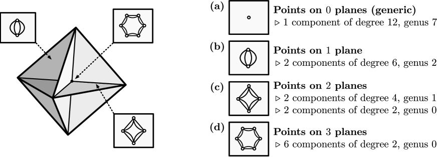
Figure 1: Moment map fibers over the chamber complex of the octahedron $\Delta(2,4)$.

• The generic fiber ${\rm Gr}(2,4)_{z}$ is an irreducible smooth curve of degree $12$ and genus $7$.

• If $z$ is in a triangle of the chamber complex, then its fiber ${\rm Gr}(2,4)_{z}$ has two irreducible components, each a curve of degree $6$ and genus $2$, which intersect in four points.

• If $z$ is on an edge, then there are four components: two $\mathbb{P}^{1}$’s and two elliptic curves.

• The central fiber ${\rm Gr}(2,4)_{z}$ is a ring of six $\mathbb{P}^{1}$’s: consecutive pairs touch at two points.

Figure 1 shows the dual graphs for the four types of fibers. Their vertices are the irreducible components of the curve. Edges represent intersections between pairs of components. Figure 2 shows the Riemann surfaces corresponding to the curves of type (a) and (d). The generic fiber (a) is a Riemann surface of genus seven. The most special fiber (d) is a ring of six Riemann spheres, touching consecutively at pairs of points. Passing to nearby generic fibers smoothes the $12$ singular points and creates the Riemann surface of genus seven.

The squaring map ${\rm Gr}(2,4)_{z}\rightarrow{\rm sGr}(2,4)_{z}$ takes our surface of genus seven onto a torus. This is the plane cubic curve in Example 6.10. By the Riemann-Hurwitz Theorem, the map has $12$ ramification points, and these correspond to the $12$ singular points seen in type (d). For the dual graph (d) in Figure 1, we obtain the natural $2$-to-$1$ map onto the hexagon.

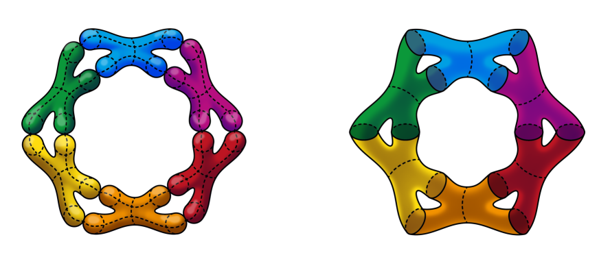
Figure 2: The fiber (d) over the midpoint of $\Delta(2,4)$, shown on the left, is a ring of six Riemann spheres. The general fiber (a), shown on the right, is a Riemann surface of genus seven.

Acknowledgment. We thank Aldo Conca for helping us with the proof of Theorem 3.4.

Authors’ addresses:

Karel Devriendt, MPI-MiS Leipzig karel.devriendt@mis.mpg.de

Hannah Friedman, UC Berkeley hannahfriedman@berkeley.edu

Bernd Sturmfels, MPI-MiS Leipzig bernd@mis.mpg.de

References

- [1] D. Agostini, T. Brysiewicz, C. Fevola, L. Kühne, B. Sturmfels and S. Telen: Likelihood degenerations, Advances in Mathematics 414 (2023) 108863.
- [2] N. Biggs: Algebraic potential theory on graphs, Bulletin London Math. Soc. 29 (1997) 641–682.
- [3] P. Breiding and S. Timme: HomotopyContinuation.jl: A Package for Homotopy Continuation in Julia, Math. Software – ICMS 2018, 458–465, Springer International Publishing (2018).
- [4] A. Conca and V. Welker: Lovász-Saks-Schrijver ideals and coordinate sections of determinantal varieties, Algebra and Number Theory 13 (2019) 455–484.
- [5] H. Friedman, B. Sturmfels and M. Zubkov: Likelihood geometry of determinantal point processes, Algebraic Statistics (2024).
- [6] I.M. Gelfand, R.M. Goresky, R.D. MacPherson and V.V. Serganova: Combinatorial geometries, convex polyhedra, and Schubert cells, Advances in Mathematics 63 (1987) 301–316.
- [7] K. Gilman, D. Tarzanagh and L. Bolzano: Grassmannian optimization for online tensor completion and tracking with the t-SVD, IEEE Trans. Signal Processing 70 (2022) 2152–2167.
- [8] D. Grayson and M. Stillman: Macaulay2, a software system for research in algebraic geometry, available at https://macaulay2.com.
- [9] J.B. Hough, M. Krishnapur, Y. Peres and B. Virág: Determinantal processes and independence, Probability Surveys 3 (2005) 206–229.
- [10] S. Hoşten and A. Khetan: Solving the likelihood equations, Foundations of Computational Mathematics 5 (2005) 389–407.
- [11] A. Kassel and T. Lévy: Determinantal probability measures on Grassmannians, Annales de l’Institut Henri Poincaré Comb. Phys. Interact. 9 (2022) 659–732.
- [12] G. Kirchhoff: Über die Auflösung der Gleichungen, auf welche man bei der Untersuchung der linearen Vertheilung galvanischer Ströme geführt wird, Annalen der Physik 148 (1847) 497–508.
- [13] Z. Lai, L.-H. Lim and K. Ye: Simpler Grassmannian optimization, (2020), arXiv:2009.13502.
- [14] L.-H. Lim, K.S. Wong and K. Ye: Numerical algorithms on the affine Grassmannian, SIAM Journal on Matrix Analysis and Applications 40 (2019) 371–393.
- [15] M. Michałek and B. Sturmfels: Invitation to Nonlinear Algebra, Graduate Studies in Mathematics, Vol 211, American Mathematical Society, 2021.
- [16] B. Sturmfels and S. Telen: Likelihood equations and scattering amplitudes, Algebraic Statistics 12 (2021) 167–186.
- [17] L. Williams: The positive Grassmannian, the amplituhedron, and cluster algebras, Proceedings of the International Congress of Mathematicians 2022, Vol 6, EMS Press (2023) 4710–4737.