Dust formation in common envelope binary interactions – II:
3D simulations with self-consistent dust formation

Abstract

We performed numerical simulations of the common envelope (CE) interaction between two thermally-pulsing asymptotic giant branch (AGB) stars of 1.7 M_⊙ and 3.7 M_⊙, and their 0.6 M_⊙ compact companion. We use tabulated equations of state to take into account recombination energy. For the first time, formation and growth of dust in the envelope is calculated explicitly, using a carbon dust nucleation network with a gas phase C/O number ratio of 2.5. By the end of the simulations, the total dust yield are $\sim 8.2\times 10^{-3}$ M_⊙ and $\sim 2.2\times 10^{-2}$ M_⊙ for the CE with a 1.7 M_⊙ and a 3.7 M_⊙ AGB star, respectively, close to the theoretical limit. Dust formation does not substantially lead to more mass unbinding or substantially alter the orbital evolution. The first dust grains appear as early as $\sim$1–3 yrs after the onset of the CE rapidly forming an optically thick shell at $\sim$10–20 au, growing in thickness and radius to values of $\sim 400-500$ au by $\sim$40 yrs. These large objects have approximate temperatures of 400 K. While dust yields are commensurate with those of single AGB stars of comparable mass, the dust in CE ejections forms over decades as opposed to tens of thousands of years. It is likely that these rapidly evolving IR objects correspond to the post-optically-luminous tail of the lightcurve of some luminous red novae. The simulated characteristics of dusty CEs also lend further support to the idea that extreme carbon stars and the so called “water fountains" may be objects observed in the immediate aftermath of a CE event.

1 Introduction

The common envelope (CE) binary interaction happens when an evolving, expanding star - such as a sub-giant, red giant branch (RGB) star, asymptotic giant branch (AGB) star, or red supergiant, transfers gas to a compact companion, which can be either a lower mass main sequence star or a more evolved white dwarf, neutron star or even a black hole. The mass transfer process tends to be unstable and lead to the formation of an extended common envelope surrounding the giant’s core and the companion. As a consequence of the exchange of energy and angular momentum, the orbital separation is rapidly, greatly reduced. The envelope can be fully ejected, in which case the binary survives, or it can lead to a merger of the companion with the core of the giant.

The CE interaction is the gateway to the formation of a number of compact evolved binaries like cataclysmic variables, X-ray binaries or the progenitors of supernova type Ia, and some black hole and neutron star binaries (Paczyński, 1971; Ivanova et al., 2013; De Marco & Izzard, 2017). Moreover, common envelope interactions are likely responsible for at least a fraction of intermediate luminosity transients (Kasliwal et al., 2011), such as luminous red novae (e.g., Blagorodnova et al., 2017) and some of these are known to produce dust (Tylenda et al., 2011; Nicholls et al., 2013).

Advances in CE simulations have resulted in an initial understanding of the energetics that drive the expansion and eventual ejection of the envelope. While dynamical ejection of the entire envelope by transfer of orbital energy appears to be problematic (but see Valsan et al., 2023), the work done by recombination energy liberated at depth shows promise as a way to enact full envelope unbinding (e.g., Ivanova et al., 2015; Reichardt et al., 2020; Lau et al., 2022).

Within this context, dust may provide an additional means to drive the CE, although it may be more or less effective depending on the type of star and interaction. Dust will also alter the opacities of the cooler parts of the CE ejecta, likely altering the appearance of the transient that results from the interaction. Past CE and other binary interaction simulations that considered dust were either 1D (Lü et al., 2013), analysed the conditions of the expanding envelope but did not calculate dust formation (Glanz & Perets, 2018; Reichardt et al., 2019), calculated dust formation in post-processing (Iaconi et al., 2019, 2020), or worked with wider binary interactions (Bermúdez-Bustamante et al., 2020).

In a recent study (González-Bolívar et al., 2023, hereafter paper I) we carried out two CE simulations with a 1.7 M_⊙ and a 3.7 M_⊙ AGB stars where the dust opacity was estimated using the simplified prescription devised by Bowen (1988). While the Bowen approximation has been tested for the case of single AGB stars (e.g. Chen et al., 2020; Bermúdez-Bustamante et al., 2020; Esseldeurs et al., 2023), it has not been used before in CE calculations. We found that dust driving has a limited effect in the unbound envelope mass. However, the opacity of the cool, expanded envelope is greatly increased by the dust.

In this simplified formulation, when the temperature drops below the condensation temperature, the opacity rapidly increases to its user-defined maximum values, while in nature we would expect a time delay between the start of dust formation and the net increase of the opacity. Finally, the Bowen approximation does not provide any information on the dust properties such as the average mass or size of the dust grains. In the present work, we therefore present, for the first time, results of self-consistent, 3D hydrodynamics simulations of dusty CEs, where dust formation is calculated self-consistently using a carbon nucleation network.

The paper is organised as follows: in Section 2 we describe the initial conditions of the binary system, together with the dust formation process and the calculation of the dust opacity. The dust distribution, properties and the evolution of the binary system, are presented in Section 3 alongside the size and shape of the photosphere. The results are discussed in Section 4 and eventually summarised in Section 5.

2 Simulation Setup

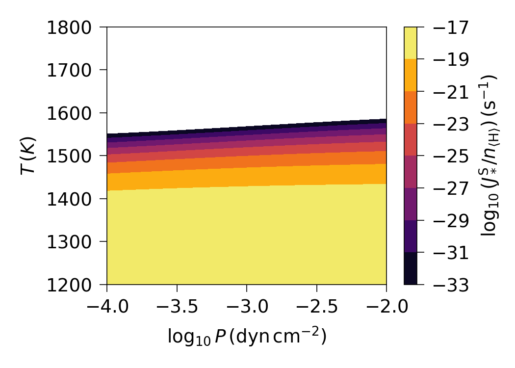
Figure 1: Color map of the normalized nucleation rate per hydrogen atom $(\widehat{J}^{S}_{*}=J^{S}_{*}/n_{\langle H\rangle})$ versus temperature and pressure, for a C/O number ratio of 2.5.

For our dusty CE simulations, we use two stellar models that were calculated using the one-dimensional implicit stellar evolution code Modules for Experiments in Stellar Astrophysics (MESA), version 12778 (Paxton et al., 2011; Paxton et al., 2013, 2015). The first model is the same as the one used by Gonzalez-Bolivar et al. (2022), namely an AGB star with a mass of 1.71 M_⊙ (zero-age main sequence mass of 2 M_⊙), a radius of 260 R_⊙, a He-rich core of 0.56 M_⊙, and at its seventh thermal pulse. The second stellar model comes from a zero-age main sequence star of 4 M_⊙  that was evolved to the fourth AGB thermal pulse, at which point it had a mass of 3.7 M_⊙, a core mass of 0.72 M_⊙ and a radius of 343 R_⊙ (for more details, see Gonzalez-Bolivar et al., 2022). Both models are placed in orbit with a 0.6 M_⊙ companion star modelled as a point particle, which can represent either a main-sequence star or a white dwarf. The simulation starts at the onset of Roche lobe overflow (at a separation of 550 R_⊙ and 637 R_⊙, for the 1.7 M_⊙ and 3.7 M_⊙ simulations, respectively), which are the separations at which the giants approximately fill their Roche lobes. Inputs and outputs of the simulations are listed in Table 1.

Model	$M_{1}$	$q$	Dust	$r_{\mathrm{soft}}$	$a_{i}$	$a_{\mathrm{f}}$	$M_{\rm ub}$
	(M⊙)			(R⊙)	(R⊙/au)	(R⊙)	(M⊙/%)
Non-dusty 1.7	1.7	0.35	No	2.5	550 / 2.6	33	0.93 / 82
Bowen 5 1.7	1.7	0.35	Bowen $\kappa_{\rm max}=5$	2.5	550 / 2.6	33	0.96 / 84
Bowen 15 1.7	1.7	0.35	Bowen $\kappa_{\rm max}=15$	2.5	550 / 2.6	40	1.01 / 88
Dusty 1.7	1.7	0.35	Nucleation	2.5	550 / 2.6	42	1.00 / 88
Non-dusty 3.7	3.7	0.16	No	8.0	637 / 3.0	10	2.47 / 83
Bowen 5 3.7	3.7	0.16	Bowen $\kappa_{\rm max}=5$	8.0	637 / 3.0	10	2.35 / 79
Bowen 15 3.7	3.7	0.16	Bowen $\kappa_{\rm max}=15$	8.0	637 / 3.0	11	2.56 / 86
Dusty 3.7	3.7	0.16	Nucleation	8.0	637 / 3.0	12	2.48 / 83

Table 1: A list of the simulations used in this study. In all cases the companion has a mass of $M_{2}=0.6$ M_⊙. The 1.7 M_⊙ (3.7 M_⊙) star had a radius of 260 R_⊙ (343 R_⊙). The first column shows the name of each simulation. The second column shows the mass of the giant donor star. The third column indicates the mass ratio, $q=M_{2}/M_{1}$. The fourth column indicates whether dust is present and the method used to calculate its opacity. The fifth column is the softening length of the point mass particles. The sixth and seventh columns are the initial separation (in R_⊙ and au) and the final orbital separation, respectively, at 12.5 years and the last column is the unbound mass by the mechanical criterion (see text) at the same time (in M_⊙ and as percentage of the envelope mass – 1.14 M_⊙ and 2.98 M_⊙ for the 1.7 M_⊙ and 3.7 M_⊙ models, respectively).

For all simulations we use the smoothed particle hydrodynamics (SPH) code phantom with $1.37\times 10^{6}$ SPH particles as was done by Gonzalez-Bolivar et al. (2022). Approximately 8.6 years after the start of the 1.7 M_⊙ model, we have modified the simulation setup, specifically we have changed the sink particle accretion radius from 0 R_⊙ (i.e., no accretion) to 15 R_⊙. The reason behind the change at that particular instant is to "remove" $\sim$6000 particles (less than 0.5% of the total SPH particles) positioned within $\sim$20 R_⊙ of the companion star’s core. The density of such SPH particles is very high, but their smoothing length is very small (equation 6 in Price et al. (2018)), which causes the timestep in the simulation to decrease to such a magnitude that the computational cost is restrictively high (see section 2.3.2 in Price et al. (2018)). By removing those particles, the timestep increases and allows the simulation to be concluded at a reasonable cost. This change in configuration does not alter the validity of our results, as we are interested in the formation of dust in the ejected material, which occurs far away from the center of mass, as shown in the next section. A study of both resolution and conservation of energy and angular momentum is provided in Appendix A to support our claim. It was not necessary to remove SPH particles in the 3.7 M_⊙ model. We use phantom’s implementation of mesa’s OPAL/SCVH EoS tables (as implemented by Reichardt et al., 2020) to account for recombination energy in this adiabatic simulation. We consider the formation of carbon-rich dust assuming a C/O number ratio of 2.5, even though both AGB stars had a C/O ratio equal to 0.32 when our MESA models stopped. Although the AGB envelope C/O ratio is different in our 3D nucleation network compared to the MESA output value, its (convective) structure is not expected to be significantly affected. It was therefore deemed superflous to alter the very uncertain convective overshooting parameter to force mesa to have a higher C/O ratio.

Our simulation includes the treatment of carbon dust nucleation and growth described in Siess et al. (2022). The dust making process takes place in two steps: i) The nucleation stage, during which seed particles form from the gas phase, followed by ii) the growth phase, where monomers (dust building blocks) accumulate on the seed particle to reach macroscopic dimensions. As a result, dust formation depends on the abundances of carbon-bearing molecules in the gas, which are obtained by solving a reduced chemical network for the carbon-rich mixture. The dust calculation is based on the theory of moments presented by Gail et al. (1984, and subsequent papers). Here we give a brief account of the salient points in the nucleation implementation, so that the reader can follow the analysis presented below. For more details, refer to Siess et al. (2022) and Gail & Sedlmayr (2013). This formalism is based on the evolution of moments, $\mathcal{K}_{i}$, of the grain size distribution $f(N,t)$ and is given, for order $i$, by:

$$\mathcal{K}_{i}=\sum_{N=N_{l}}^{\infty}N^{i/3}f(N,t),$$ (1)

where $N$ is the number of monomers in a grain (typically C, C₂, C₂H and C₂H₂) and $N_{l}\sim 1000$ the minimum number of monomers that a cluster must contain to be considered as a dust grain. The knowledge of the moments gives direct access to the dust properties, for example the average grain radius:

$$\langle r\rangle=a_{0}\frac{\mathcal{K}_{1}}{\mathcal{K}_{0}},$$ (2)

where $a_{0}=1.28\times 10^{-4}$ $\mu$m is the radius of a monomer inside a dust grain, namely that of a carbon atom. The equations governing the evolution of the moments are given by:

$$\frac{\mathrm{d}\widehat{J}_{*}}{\mathrm{d}t} = \frac{\widehat{J}_{*}^{s}-\widehat{J}_{*}}{\tau_{*}},$$ (3)

$$\frac{\mathrm{d}\widehat{\mathcal{K}}_{0}}{\mathrm{d}t} = \widehat{J}_{*},$$ (4)

$$\frac{\mathrm{d}\widehat{\mathcal{K}}_{i}}{\mathrm{d}t} = \frac{i\,\widehat{\mathcal{K}}_{i-1}}{3\tau}+N_{l}^{i/3}\widehat{J}_{*},$$ (5)

where $\widehat{J}_{*}$ is the nucleation rate, i.e., the volumetric rate of formation of the seed nuclei, $\widehat{J}^{S}_{*}$ is its quasi-stationary value, and $\tau_{*}$ is the nucleation relaxation time towards equilibrium (for details, see Siess et al., 2022). The variable $\tau$ is the timescale for growth ($>0$) or evaporation ($<0$) of the grains and $\widehat{{\cal K}_{i}}={\cal K}_{i}/n_{\langle\mathrm{H}\rangle}$ is the normalized moment with $n_{\langle\mathrm{H}\rangle}$ the number of H atoms per unit volume. The dependence of the nucleation rate on temperature and pressure for our adopted C/O = 2.5 is illustrated in Figure 1 and peaks around 1100-1400 K over a wide range of pressures, $P$, between $10^{-10}$ and $\rm 10~{}dyn\,cm^{-2}$.

Another important parameter is the supersaturation ratio $S$, given by

$$S=\frac{P_{\mathrm{C}}(T_{\mathrm{g}})}{P_{\mathrm{sat}}},$$ (6)

where $P_{\mathrm{C}}(T_{\mathrm{g}})$ is the partial pressure of carbon in the gas phase, $P_{\mathrm{sat}}$ is the vapor saturation pressure of carbon in the solid phase and $T_{\mathrm{g}}$ is the gas temperature. For nucleation to occur, $S$ must be larger than a critical value $S_{c}$, of the order of unity, and this happens when the temperature drops below $\sim 1500$ K.

The gas opacity is set to a constant value of $2\times$10^-4 cm² g^-1, which is a good approximation at temperatures below $10^{4}$ K, where hydrogen is mostly recombined (Siess et al., 2022). The Planck mean opacity $\kappa_{\mathrm{d}}$ of each particle is calculated in the framework of the Mie theory using the following expression

$$\kappa_{\mathrm{d}}=\frac{\pi a_{0}^{3}}{\rho}Q^{\prime}_{\mathrm{ext}}{\mathcal{K}_{3}},$$ (7)

where $\rho$ is the gas density and $Q^{\prime}_{\mathrm{ext}}=6.7\,(T_{\mathrm{d}}/\mathrm{K})$ cm^-1 is a fit of the Planck mean of the extinction coefficient in the small particle limit. This simple expression for $Q^{\prime}$ depends only on the dust temperature $T_{\mathrm{d}}$ and is strictly valid for grain sizes $a\lesssim 0.1\mu m$ (for details, see Sect 3.2.2 of Siess et al. 2022 and Sect 7.5.5 of Gail & Sedlmayr 2013).

In the absence of a proper treatment of radiative transfer in our simulations, we will assume that gas and dust are thermally coupled, i.e. $T_{\mathrm{g}}=T_{\mathrm{d}}=T$. The dust mass is the sum over all the SPH particles of the average mass of carbon atoms condensed in dust and is given by

$$\mathrm{M}_{\rm dust}=\sum_{\mathrm{part.}}\frac{m_{\mathrm{SPH}}}{\bar{m}_{\mathrm{H}}}m_{c}\,\widehat{K}_{3},$$ (8)

where $\widehat{K}_{3}$ is the average number of condensed carbon atoms per H-atoms for each SPH particle, $m_{c}$ the mass of a carbon atom and $m_{\mathrm{SPH}}$ is the (constant) mass of an SPH particle. The mean mass per hydrogen atom is given by

$$\bar{m}_{\mathrm{H}}=m_{u}\,\sum_{i}\,A_{i}\,\epsilon_{i},$$ (9)

where $\epsilon_{i}$ is the abundance by number relative to hydrogen, $A_{i}$ is the atomic weight of chemical element $i$ and $m_{u}$ the atomic mass unit.

The knowledge of the dust opacity allows us to calculate the radiative acceleration on the particles as an additive term to the equation of motion which becomes

$$\frac{d\mathbf{v}}{dt}=-\frac{\nabla P}{\rho}-\nabla\phi_{\mathrm{gas-gas}}-\nabla\phi_{\mathrm{sink-gas}}+\frac{(\kappa_{g}+\kappa_{\mathrm{d}})L}{4\pi r^{2}c}\frac{\mathbf{r}}{r},$$ (10)

where $P$ is the pressure, $\phi_{\mathrm{gas-gas}}$ and $\phi_{\mathrm{sink-gas}}$ are the gravitational potentials from the SPH particles (self-gravity) and between a particle and the sink masses. The variable $r$ is the distance from the AGB core, which is assumed to produce a constant luminosity $L=5180$ L_⊙ for the 2 M_⊙ model and 9010 L_⊙ for the 4 M_⊙.

3 Results

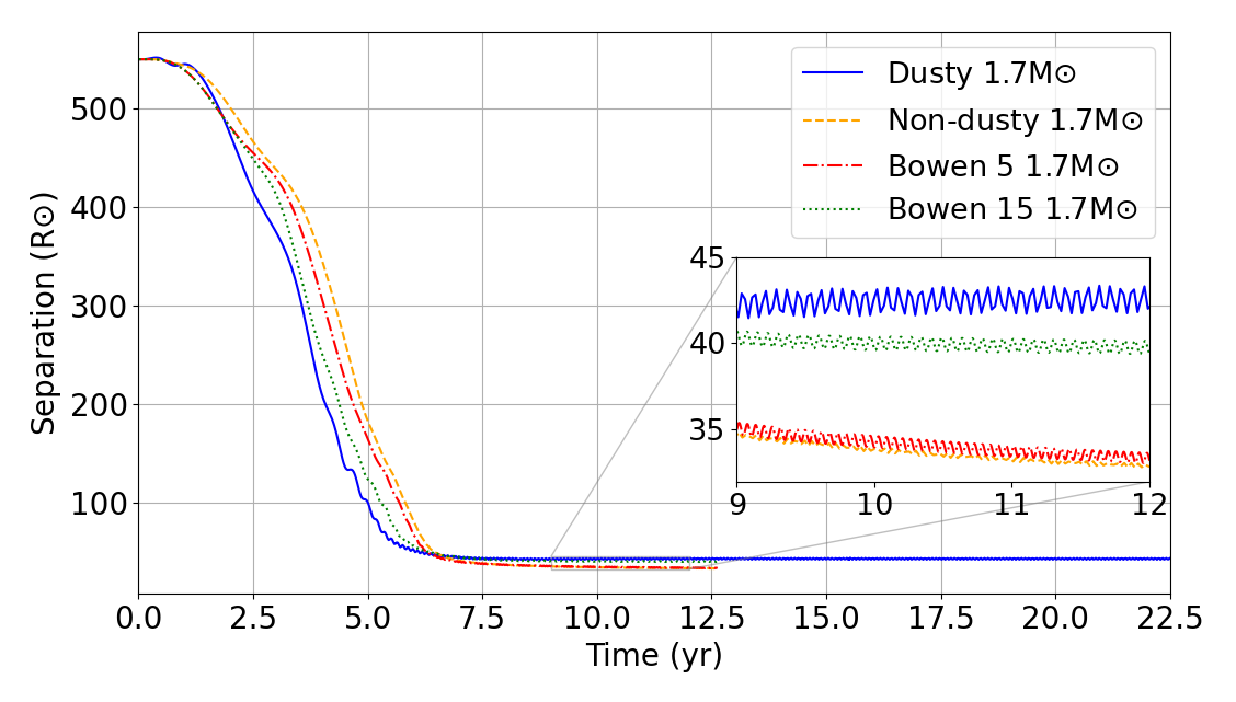
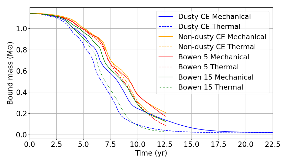
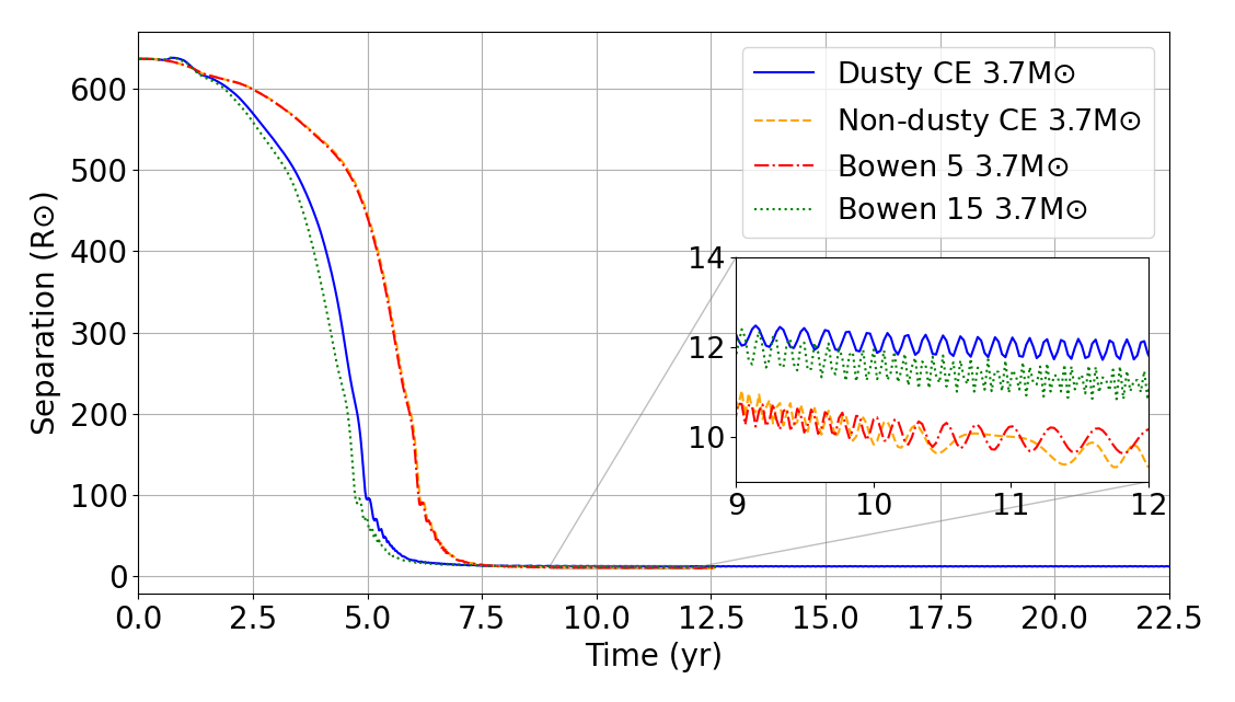
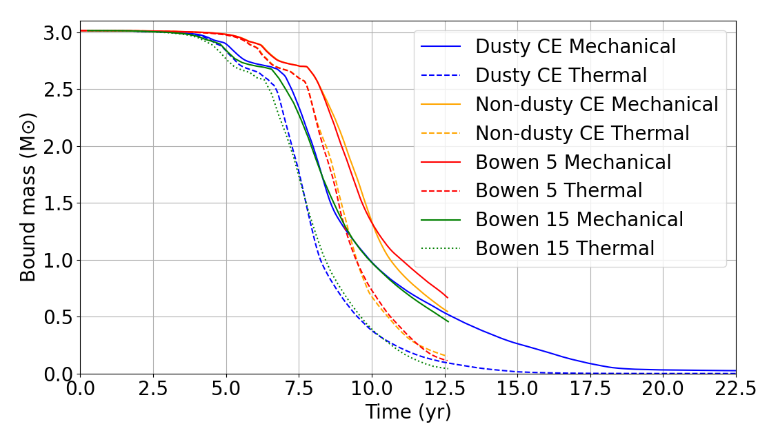
Figure 2: Orbital separation (left panels) and bound mass (right panels) as a function of time for CE simulations with a 1.7 M_⊙ (top) and a 3.7 M_⊙ (bottom) AGB primary star. During the CE evolution, dust was taken into account either by the explicit calculation of dust nucleation and growth (blue lines) or using the Bowen’s formulation described in Paper I, with a maximum opacity of $\kappa_{\mathrm{max}}=5~{}\mathrm{cm^{2}\,g^{-1}}$ (red lines) or $\kappa_{\mathrm{max}}=15~{}\mathrm{cm^{2}\,g^{-1}}$ (green lines). Also included are the CE simulations without dust (yellow lines). The insert in the left panels shows the orbital separation at the end of the in-spiral phase. The bound mass in the right panels is calculated using the mechanical criterion (solid lines) and the thermal criterion (dashed lines).

The CE in-spiral and envelope ejection in our dusty simulations proceed similarly to the non-dusty simulations of Gonzalez-Bolivar et al. (2022) and to the Bowen dust simulations of Paper I. In Section 3.1 we describe the properties of the dust that is formed in the ejected envelope, such as its opacity or the size distribution of its grains. To anchor these dust formation processes to the in-spiral timeline, we show here Figure 2, which displays the orbital evolution of all our simulations, as well as how the mass is unbound, but we will provide more details on the in-spiral and mass unbound in the presence of dust in Section 3.2.

3.1 The Dust Properties

3.1.1 Nucleation, growth and opacity of dust grains

In Figures 3 and 4 we show snapshots at different times of the supersaturation ratio, $S$, the normalized nucleation rate, $\hat{J}_{*}$, and the dust opacity, $\kappa_{\mathrm{d}}$, for the CE simulation with a 1.7 M_⊙ and a 3.7 M_⊙ AGB star, respectively. The quantities $S$, $\hat{J}_{*}$ and $\kappa_{\mathrm{d}}$ trace where the dust seeds are more likely to form, where nucleation is actually happening, and where dust has formed, respectively. To aid the visual comparison, all of the snapshots include the same temperature contours, which are equally spaced in linear scale from 2000 K (innermost) to 750 K (outermost). The $x$ and $y$ axes define the binary system’s orbital plane while the $z$ axis is perpendicular to that plane.

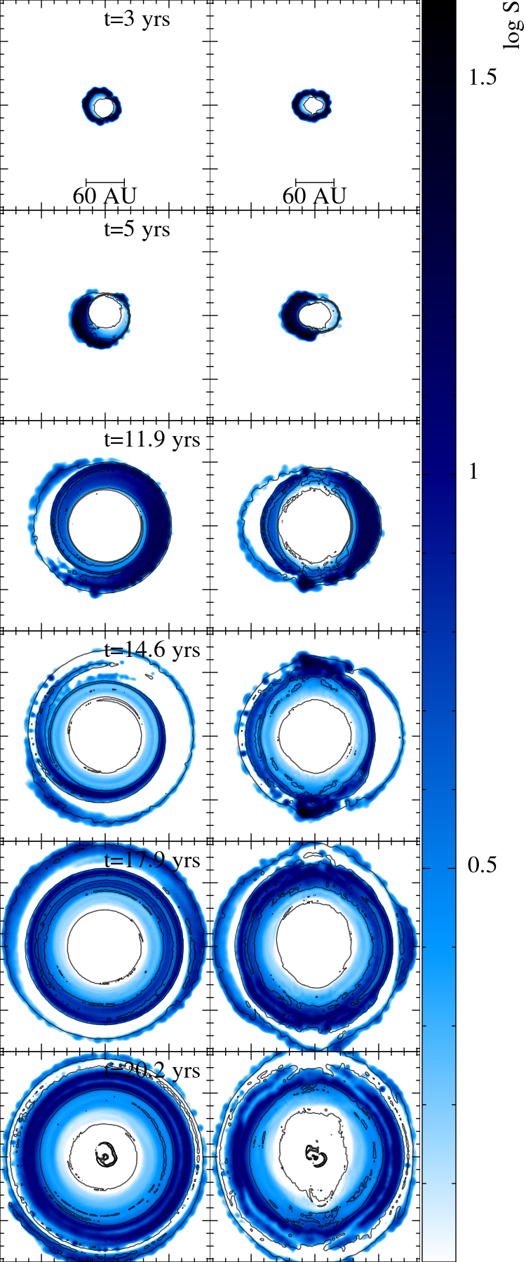
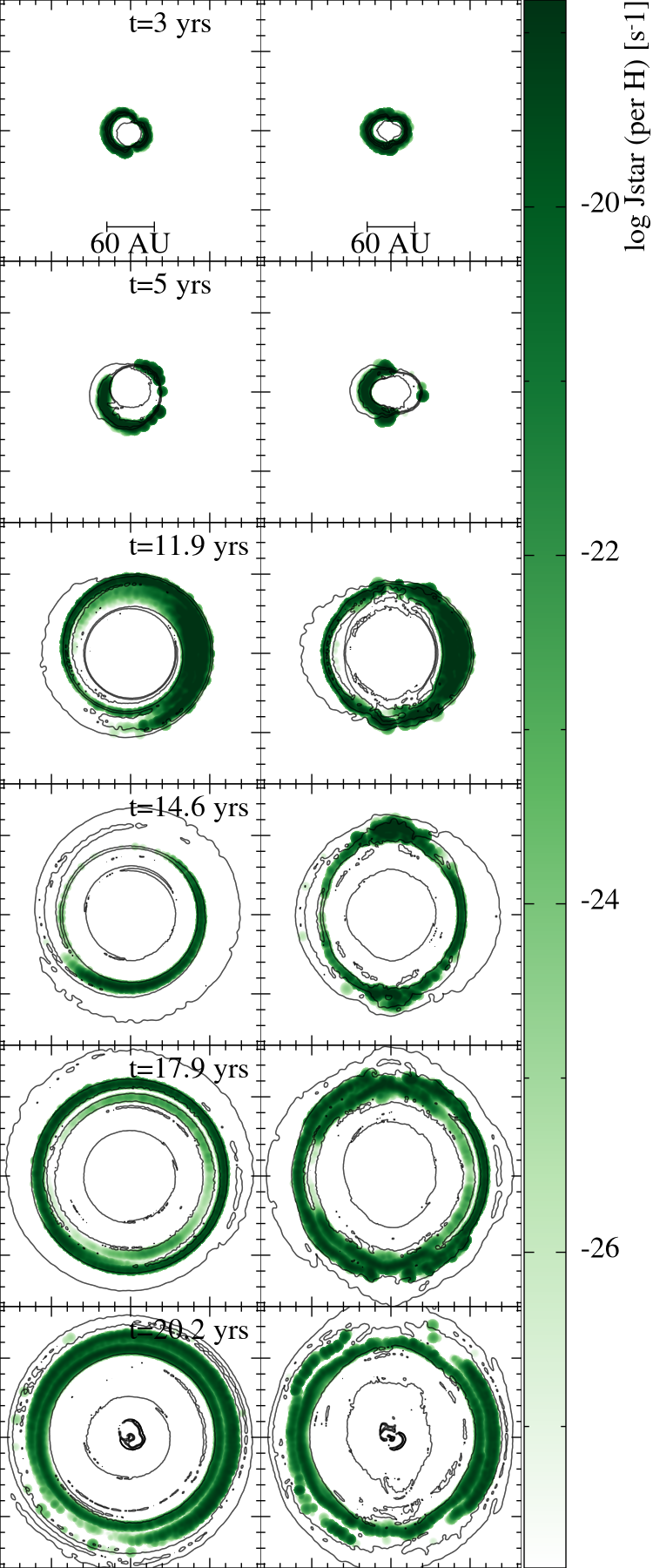
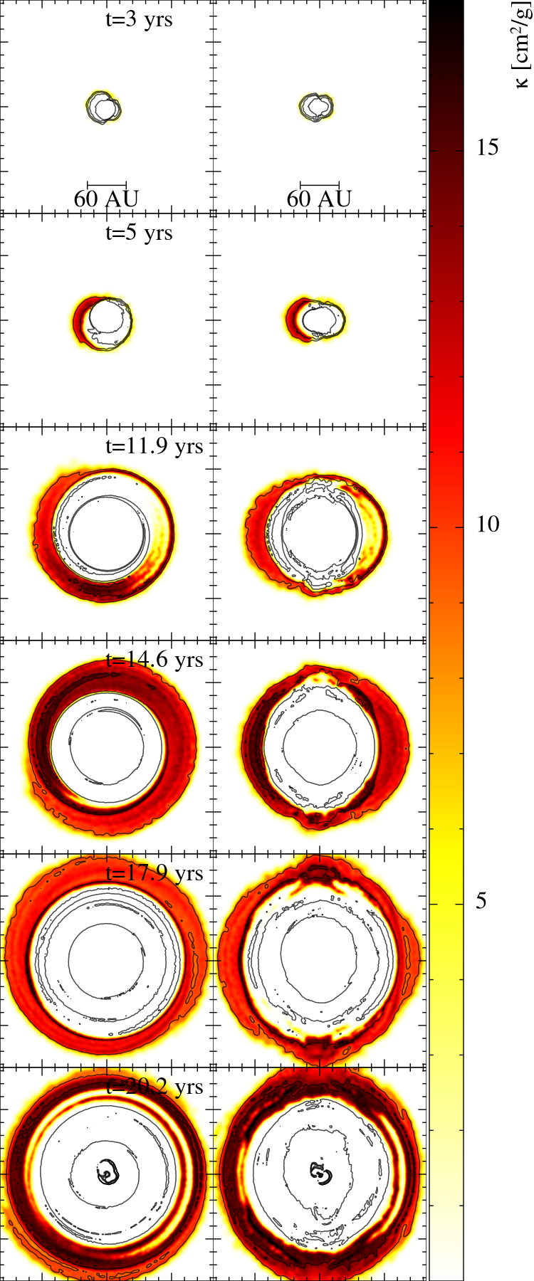
Figure 3: Slices in the XY (columns 1, 3 and 5) and XZ (columns 2, 4 and 6) planes of supersaturation ratio, $S$ (blue), nucleation rate per hydrogen atom, $\hat{J}_{\star}$ (green) and opacity, $\kappa$ (red) at 6 different times for the 1.7 M_⊙ model. Black temperature contours are equally spaced in linear scale and range between 750 K (outermost contour) to 2000 K (innermost contour). Each panel is 160 by 160 au per side. All figure movies can be found at the following URL: https://tinyurl.com/y455avdj

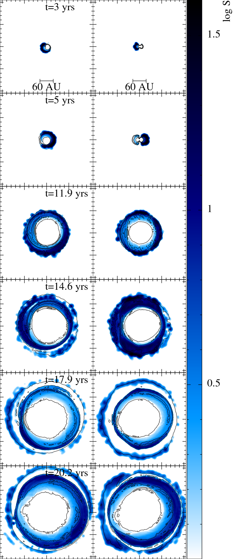
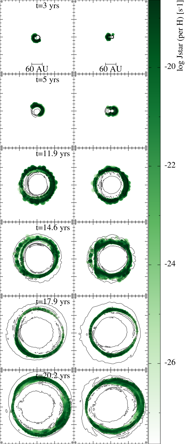
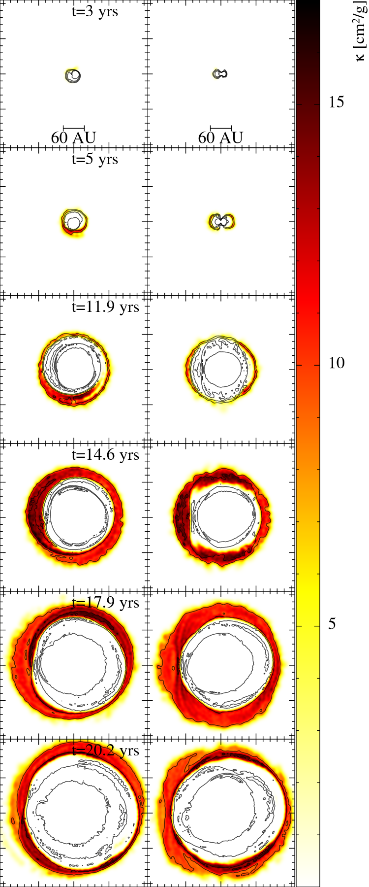
Figure 4: Slices in the XY (columns 1, 3 and 5) and XZ (columns 2, 4 and 6) planes of supersaturation ratio, $S$ (columns 1 and 2), nucleation rate per hydrogen atom, $\hat{J}_{\star}$ (columns 3 and 4) and opacity, $\kappa$ (columns 5 and 6) at 6 different times for the 3.7 M_⊙ model. The temperature contours and the scale bar are the same as in Figure 3. All figure movies can be found at the following URL: https://tinyurl.com/y455avdj

The dust nucleation rate starts to increase after the supersaturation ratio has exceeded the threshold value $S_{c}$. As a consequence, the regions with high values of $J_{*}$ are typically associated with those of high $S$ (Figures 3 and 4). At early times (3 and 5 years), the efficient formation of dust seeds ($S>10$ and $\hat{J}_{*}>10^{-22}$) takes place in the XY plane in lumpy arcs or crescent shapes around the center of mass. In the XZ plane, the regions of seed formation are asymmetric and elongated in the orbital direction, with one side being more efficient than the other. This asymmetry is likely due to the initial mass-loss through the outer Lagrange points, which causes at early times dense spiral outflows where dust can be formed more efficiently. At later times (after 11.9 yrs), the regions of seed formation tend to be more regular in shape (quasi-spherical) and appear as shells in both models (the lumpy appearance at larger radii is due to low numerical resolution).

Regarding the $\kappa_{\mathrm{d}}$ distribution, dust formation occurs as early as $\sim$1 yr from the onset of simulations, at a distance of $\sim$10 au from the center of mass. However, it is only after $\sim$3 years that a shell of high opacity ($\kappa_{\mathrm{d}}>$ 5 cm² g^-1) can be seen surrounding the stars. For the 1.7 M_⊙ simulation, the dusty shell at 11.9 yrs is very thin in some parts and is at $\sim 100$ au from the center of mass. With time, its thickness increases (especially at 14.6 and 17.9 yrs) and becomes more uniform. At 20 yrs the dusty shell’s radius has increased to $\sim 160$ au. For the 3.7 M_⊙ simulation, at 11.9 yrs the dusty shell is also located $\sim 100$ au from the center of mass and its thickness increases between 14.6 and 17.9 yrs. However, in contrast to the lower mass simulation, at 20 yrs the shell has a radius of $\sim 200$ au.

In the 1.7 M_⊙ simulation the dusty shell is thicker and is elongated in the polar direction, with the development of bulges. In the higher mass model, such polar protuberances are absent and the dusty envelope maintains a more spherical shape. These differences in the geometry of the dusty shell may be related to the differences in orbital separation and mass ratio between the two models, which affect the mass ejection geometry and thus the dust distribution.

In general, regions with high values of $\kappa_{\mathrm{d}}$ are located outside the regions with high values of $\hat{J}_{*}$, and this is because it takes time for the opacity to increase after the gas reaches the condensation temperature. In Figure 5, the SPH particles are colored according to the time at which dust formation occurrs as indicated by the ratio of the normalised moments, ${\widehat{\cal K}_{3}}/{\widehat{\cal K}_{0}}$, which represents the amount of condensed carbon atoms per dust grain.

From Figure 5 it is clear that the opacity peaks at $\sim$17-20 cm² g^-1 in both simulations. However, as the envelopes expand, their density and temperature decrease. In such low-density regions, dust growth (which occurs through the collision of monomers with dust grains) stops because of the rarefaction of monomers. Under such circumstances, the number of condensed carbon atoms per gram in the dust, $\mathcal{K}_{3}/\rho$, is constant. So according to Eq. 7, the opacity becomes a simple linear function of the temperature and thus decreases with the expanding cooling gas.

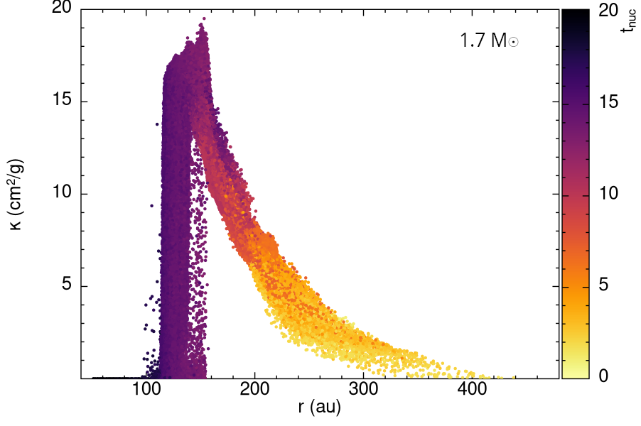
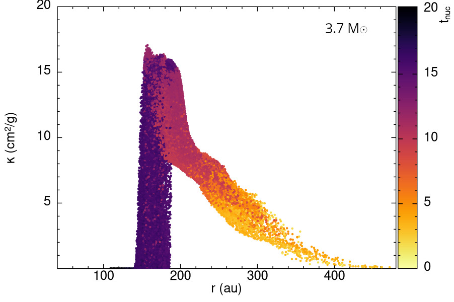
Figure 5: Dust opacity versus distance for the 1.7 M_⊙ (left) and 3.7 M_⊙ (right) model at 20.2 years from the start of the simulations. The color map indicates nucleation time $t_{\rm nuc}$, the time (in years) when dust was formed in the SPH particles. A movie of this figure can be found at the following URL: https://tinyurl.com/y455avdj

In the Bowen approximation of Paper I, the opacity reaches its maximum, user defined value, $\kappa_{\mathrm{max}}$, as soon as the temperature drops below the condensation threshold and remains constant as the envelope expands, which is not the case in our formalism because of the temperature dependence of $Q^{\prime}_{\mathrm{ext}}$ in Eq. 7. As a result, using the Bowen approximation leads to more opaque inner regions (as clearly seen in Figure 6), over estimation of dust production and potentially more acceleration by radiation pressure, which has been included both in this paper and in Paper I.

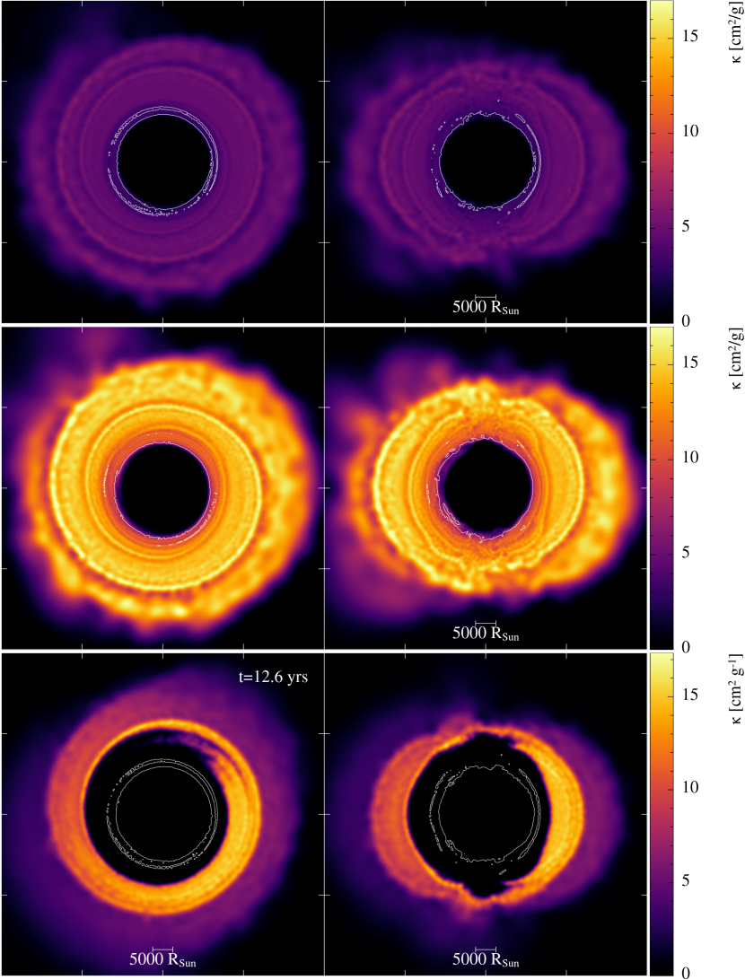
Figure 6: Equatorial and perpendicular slices of opacity at 12.6 years for the 1.7 M_⊙ Bowen simulations (González-Bolívar et al., 2023) with $\kappa_{\rm max}=5$ cm² g^-1 (top row) with $\kappa_{\rm max}=15$ cm² g^-1 (middle row) and with dust nucleation (bottom row).

Figure 7 shows the expansion of the envelope, with a similar colour bar as that in Figure 5. The first particles to form dust (lighter colours) are located farther away from the stars than those formed more recently (darker colours). However, this is not always the case, as illustrated in the inner regions of the 1.7 M_⊙ model where particles with dust formed at different times appear mixed. For the 3.7 M_⊙ model, the times at which dust formed show a more clearly decreasing sequence with radius. The inner structure is also less symmetric and a clear polar elongation is absent. These asymmetries occur however at late times ($t_{\mathrm{nuc}}\gtrsim 30$ yr) in the unbound mass. All of the above shows that there is no simple relationship that indicates when the dust forms as a function of its distance from the binary system, but rather that the formation of dust in certain regions depends on complex hydrodynamic interactions that occur in the ejected material during the in-spiral phase — namely, the passage of spiral shocks through the material driven by the binary interaction. A similar result was found by Iaconi et al. (2020, see their figure 2).

As already shown in Figures 3 and 4, dust nucleation does not take place throughout the entire volume of the envelope, but only in the innermost regions where suitable thermodynamic conditions are met. In Figure 8, we plot the pressure and temperature of SPH particles when they reach a threshold opacity $\kappa_{\mathrm{d}}=0.02$ cm² g^-1 (one hundred times larger than for the gas). Most of the particles form dust in a fairly narrow region of temperature around $\sim 1400$ K, with a spread of $\lesssim 100$ K. By comparing Figure 8 with Figure 1 it is clear that dust formation occurs at the intersection between higher theoretical rates and adequate conditions.

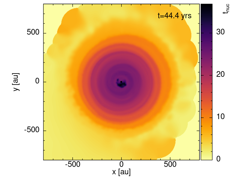
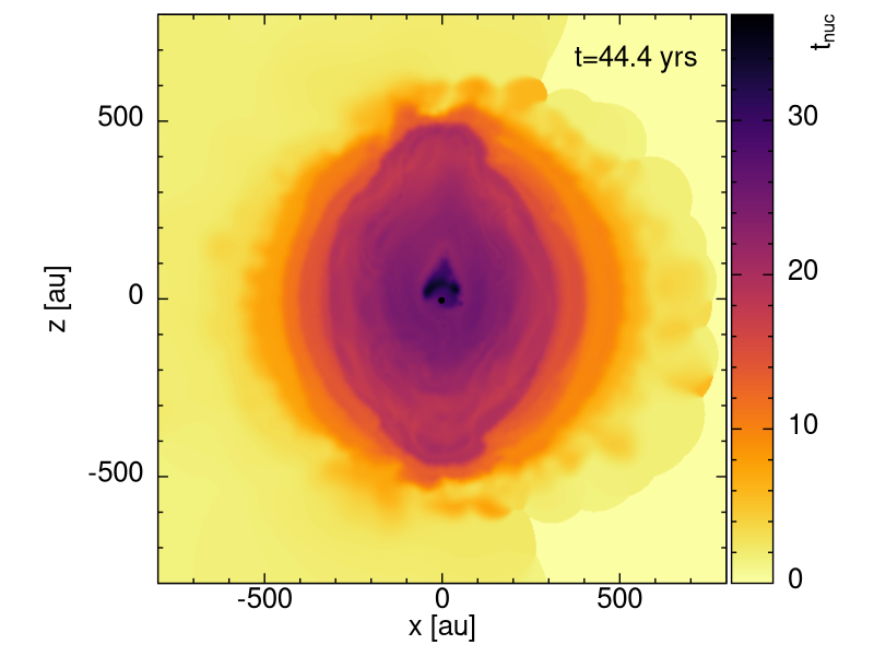
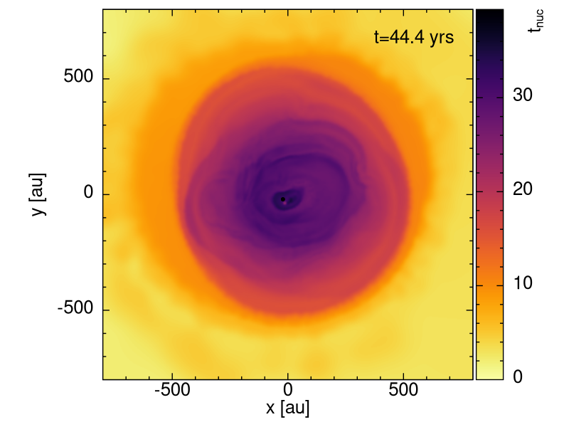
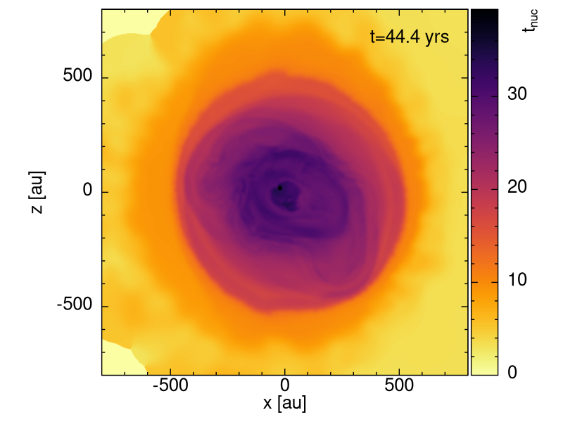
Figure 7: Colour map of nucleation time $t_{\rm nuc}$ in the XY (left column) and XZ plane (right column), for the 1.7 M_⊙ (top row) and 3.7 M_⊙ (bottom row) model, after 44.4 yrs of simulation. A movie of this figure can be found at the following URL: https://tinyurl.com/y455avdj

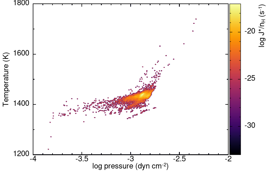
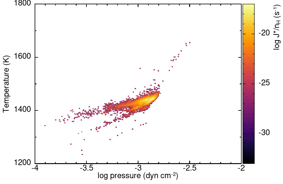
Figure 8: Temperature vs. pressure for SPH particles with dust opacity $\kappa_{\mathrm{d}}=0.02-0.025$ cm² g^-1. The color map is the normalized nucleation rate $J_{*}/n_{\langle\mathrm{H}\rangle}=\hat{J}_{*}$, and indicates where dust is forming at the largest rate. The plot is a collection of dusty SPH particles at all times during the CE simulations, from beginning to end. The left (right) panel corresponds to the 1.7 M_⊙ (3.7 M_⊙) model.

3.1.2 Dust size

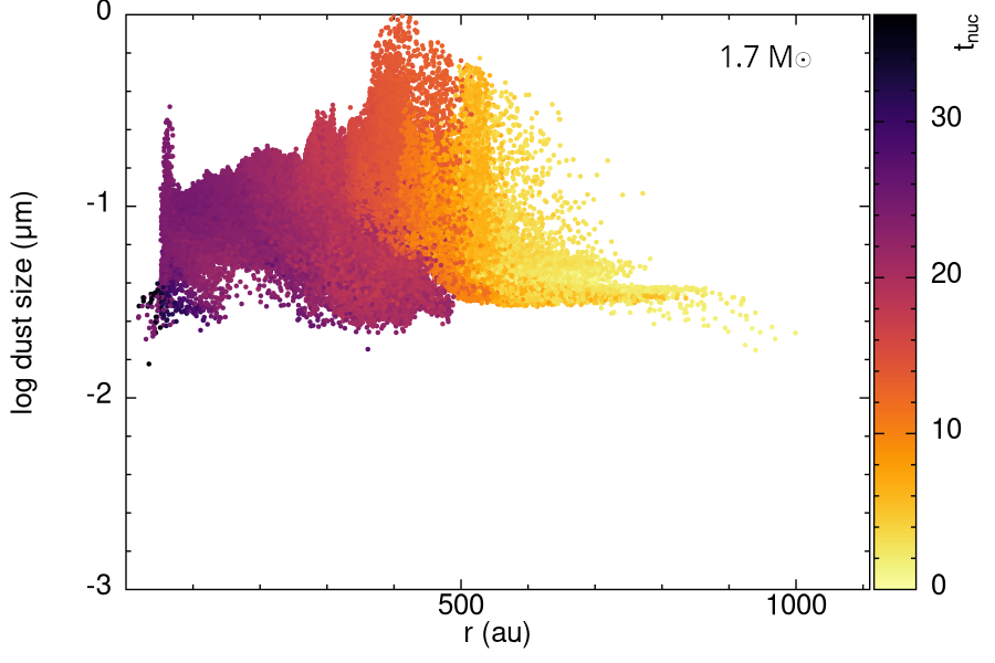
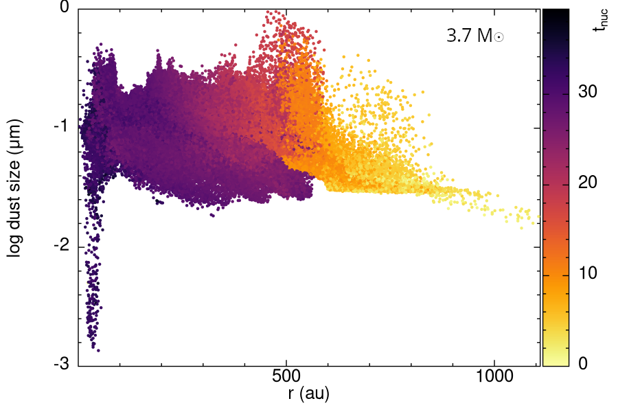
Figure 9: Average dust grains size versus distance from the centre of mass, for the 1.7 M_⊙ (top) and 3.7 M_⊙ (bottom) models, after 44.4 years of simulation. The color map indicates nucleation time in years. A movie of this figure can be found at the following URL: https://tinyurl.com/y455avdj

Figure 9 shows the average size of dust grains in each SPH particle as a function of radius, $\sim$44 years after the start of the simulations. The different colors indicate the time with respect to the start of the simulations at which dust formation happened, with younger dust as we move from lighter to darker colours (as per the colour bar in Figure 5). For the 1.7 M_⊙ model, this figure, and the associated movie, show that dust is forming in the inner regions of the envelope (10-20 au) with small grains ($10^{-3}$ $\mu$m) that rapidly increase in size to $\sim 1\mu$m. Depending on the time of formation, dust grows to different maximum sizes: early dust (yellow colour in Figure 9) forms grains in a narrow range of sizes (0.03 - 0.04 $\mu$m), while later dust, particularly that formed at $\sim$12 yrs, has a range in size between 0.03 and 1 $\mu$m.

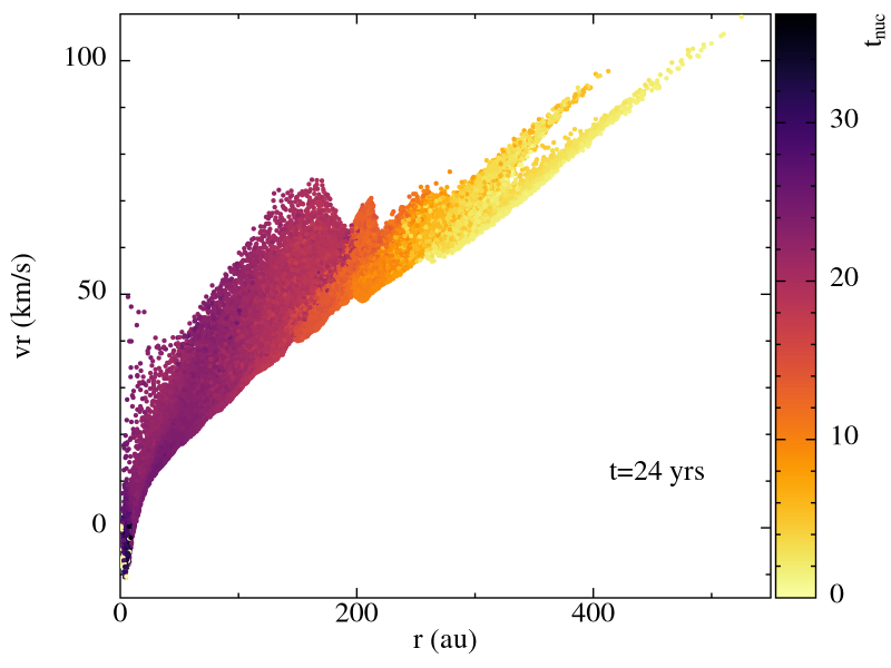
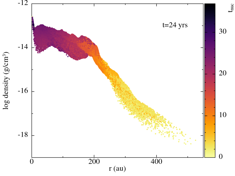
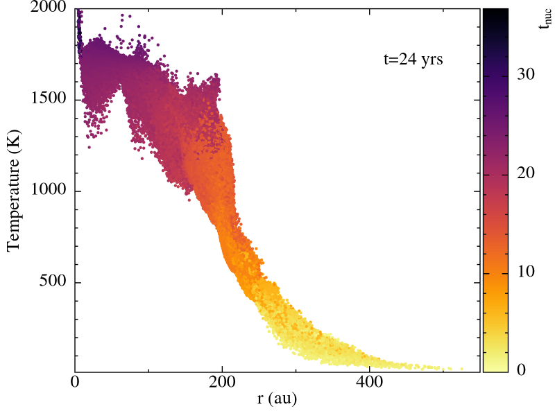
Figure 10: Velocity (top), density (middle) and temperature (bottom) versus distance from the centre of mass, for the 1.7 M_⊙ model after 24 years. Similar results are obtained with the 3.7 M_⊙ model. Movies of these figure panels can be found at the following URL: https://tinyurl.com/y455avdj.

The formation shell also varies in size and radius over time as clearly seen in the movies. For the 1.7 M_⊙ model, the initial shell is thin and very close to the centre ($\sim$10-20 au). At later times ($\sim$21 yrs) it is broader and farther out ($\sim$70-170 au). Later on, at $\sim$22 yrs, formation resumes in the innermost shell ($\sim$10-20 au), and at 24 years formation takes place in a wide shell ($\sim$10-200 au). Eventually ($\sim$30 yrs) formation slows down and remains localised in two thin shells (10-20 and 120-130 au), ceasing in the outer shell shortly thereafter, but persisting in the inner shell till about 38 years, after which formation stops altogether.

For the 3.7 M_⊙ model, dust formation starts at $\sim$1.5 yrs at a similar location (10-20 au) to the 1.7 M_⊙ model. Early dust has a narrow range in size around $\sim$0.6 $\mu$m. Later dust has a range in size between 0.6 and 1 $\mu$m, with the dust that achieves the largest range, again, formed at about 15 yrs. At $\sim$13 yrs the formation of dust decreases with production restricted to a thin shell ($\sim$80-100 au). By $\sim$22 yrs the dust-forming shell has broadened to between $\sim$100 and $\sim$200 au and by $\sim$26 years production starts in a second, inner shell ($\sim$10-20 au), while massive production continues in a shell between $\sim$100 and $\sim$150 au. By $\sim$28 years dust production is copious and in a shell between $\sim$10 and $\sim$180 au. By $\sim$31 years production retreats into a shell between $\sim$10 and $\sim$130 au, with this shell thinning out into a smaller range 30-50 au. Interestingly, at the very end of the simulation, ($\sim$43 years), dust formation resumes in the thin shell near the centre, but at a lower rate.

Our formalism does not include dust destruction but the average grain size in an SPH particle can decrease, if newly formed small grains are being produced. This explains why the average grain size distribution of Figure 9 is not increasing with time.

Early dust grows to a smaller size than late dust because, as shown in Figure 10 (a snapshot of dusty particles temperature, velocity and density at 24 years), the velocity of the flow is inversely proportional to the nucleation time, i.e., late dust forms in slower moving regions and has more time to grow. The dust reaches its maximum size after $\sim 12$ years and afterwards the growth slows down because the temperature profile becomes flatter. In other words, as the gas expands it does not cool as fast as earlier on, which hinders dust growth.

Figure 11 displays histograms of the average dust grain size in each SPH particle, at three different times for the 1.7 M_⊙ and 3.7 M_⊙ simulations. For the 1.7 M_⊙ model the range of dust sizes at 7 and 20 yrs remains approximately 0.002 - 0.6 $\mu$m, which, by 40 years, grows to 0.02 - 1 $\mu$m. The 3.7 M_⊙ model is quite different: the range of sizes at 7 yrs is narrower (0.002 - 0.15 $\mu$m) increasing to 0.004-0.7 $\mu$m. It then widens to 0.002-1 $\mu$m, indicating that between 7 and 44 years there was a decrease in the dust formation rate also seen in the movie. The peak of the dust distribution is very similar in the two models: 0.04 $\mu$m at 7 years, 0.05 - 0.07 $\mu$m at 20 years and 0.05 - 0.2 $\mu$m at 44 years.

At the end of the simulations, the largest average grain sizes are approximately 0.8-1.0 $\mu$m. The distributions are characterized by an initial positive slope, with the number of grains increasing with grain size from $\approx 0.001$ up to $\approx 0.05$ $\mu$m, then a plateau up to $\sim$0.1 and 0.15 $\mu$m for the 1.7 M_⊙ and 3.7 M_⊙  models, respectively, and finally a decrease in the number of SPH particles as a function of the average grain size. Fitting the distribution with

$$n(a_{\rm ave})=Ca_{\rm ave}^{-q}$$ (11)

where $a_{\rm ave}$ is the average grain size in each SPH particle in $\mu$m. We find $q=8.2$ for both models by fitting the slope by eye (red line in Figure 11) and $C=1.5\times 10^{36}$ for the 1.7 M_⊙ model, while $C=3.6\times 10^{36}$ for the 3.7 M_⊙ model. This result is comparable to that of Iaconi et al. (2020), who find their (carbon) grain size distribution to always have a negative, albeit changing, slope, where the largest grains have a slope of $q=6.6$, only slightly smaller than for our models. The difference is not substantial when we consider that (i) the structure of the donor star used by Iaconi et al. (2020) is an RGB star of 0.88 M_⊙ and 83 R_⊙, which changes the structure of the outflow and thus the growth of dust grains in it, (ii) the dust formation model was a non-steady-state process described by Nozawa & Kozasa (2013), contrary to our formation model described in Gail & Sedlmayr (2013), which assumes chemical equilibrium.

While the dust size distribution is only the distribution of the average grain size in each SPH particle, it is notable that the steepness of the slope is much larger than interstellar dust grains assuming an MRN distribution (Mathis et al., 1977).

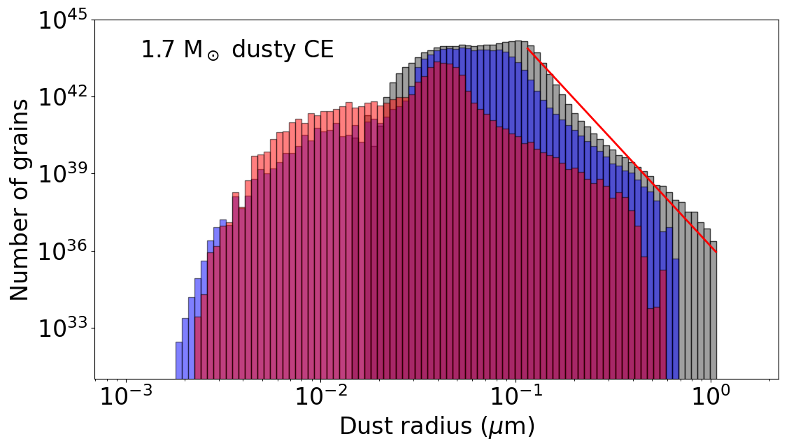
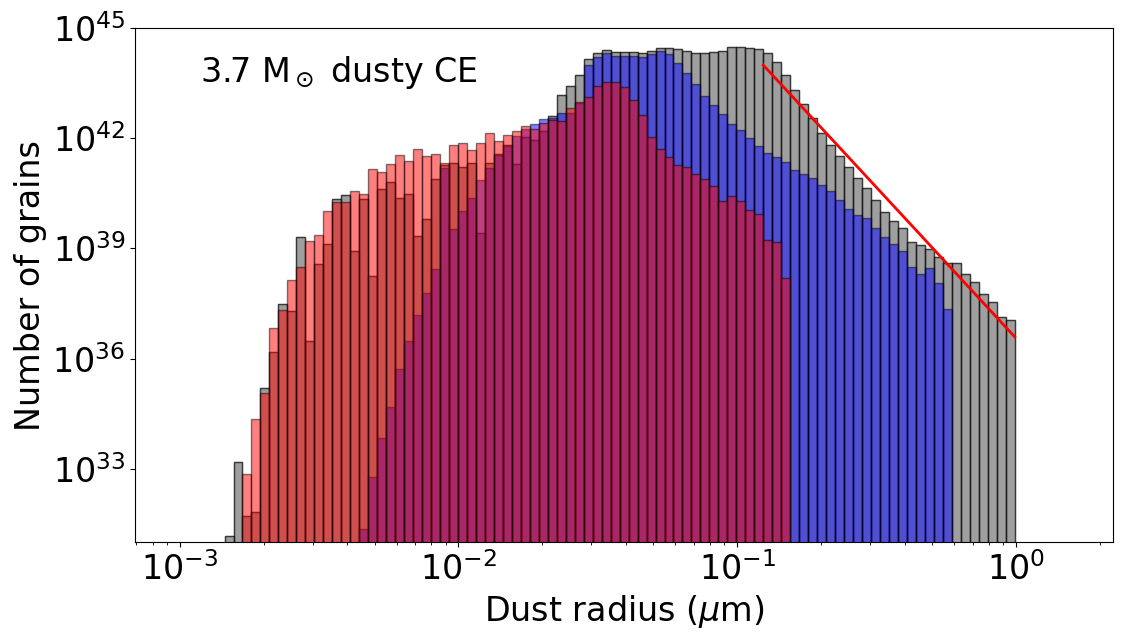
Figure 11: Histograms of the average dust grain size in each SPH particle, not the individual grain size. The pink, blue and gray histograms are at $t=7.0$ yr, $t=20$ yr and $t=44$ yr from the start of each simulation, respectively. We fit the gray histogram data using a power law, depicted here using a red line. We note that this may not correspond to the grain size distribution and cannot therefore be directly compared to, for example, MRN (Mathis et al., 1977).

3.1.3 Dust mass

Figure 12 shows the evolution of the total dust mass (Eq. 8) for the two simulations. The dust mass increases steadily until it reaches a plateau. For the 1.7 M_⊙ model this happens at $\sim$32 yrs and at a value of 0.008 M_⊙. For the 3.7 M_⊙ model it takes place at 38 yrs and with a value of 0.022 M_⊙. Thus, after 40 yr, the 1.7 M_⊙ (3.7 M_⊙) model has produced roughly four (ten) times more dust than during the first 20 years. This drastic increase is a consequence of a large fraction of the expanding envelope reaching temperatures below the condensation threshold (see Sect. 3.3). These features are related to the evolution of the grain size distribution mentioned before (Fig. 11). When nucleation is efficient (i.e., when there is a large number of small dust grains), a lot of monomers are available and contribute to dust growth producing the increase in the dust mass. With gas expansion, the nucleation rate decreases, fewer monomers are formed and dust production is consequently reduced. The dust mass produced by the models is not a function of resolution as we demonstrate in the resolution test presented in Appendix A.

Although it is difficult to establish a pattern using only our two models, we see that the more massive the donor star forms dust for longer, taking about $\sim$40 years instead of $\sim$30 years to stop making dust and making three times more dust overall.

Finally, comparing our result with those of Iaconi et al. (2020) for carbon grains, we see that the amount of dust formed in the 1.7 M_⊙ simulation is four times larger for a star twice as massive. In their simulation the total dust mass plateaus at $\sim 2.2\times 10^{-3}$ M_⊙ after $\sim$14 years for a 0.88 M_⊙ RGB star, which started off with a radius of 83 R_⊙.

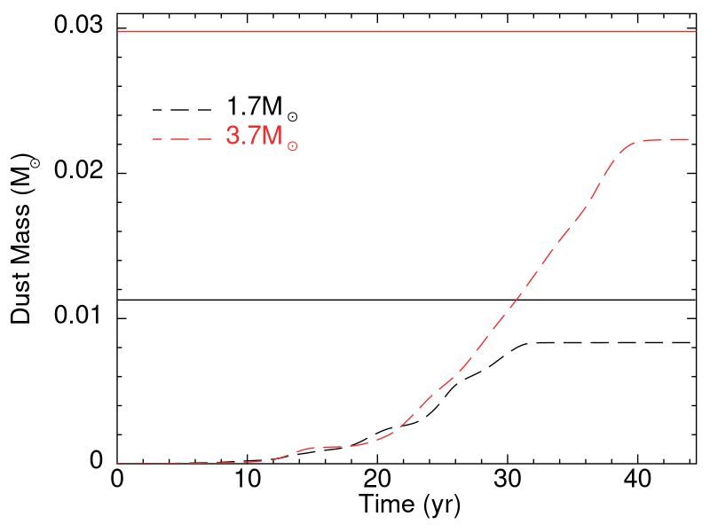
Figure 12: Total dust mass as a function of time for the 1.7 M_⊙ (black dashed line) and 3.7 M_⊙ (red dashed line) models. The horizontal lines indicate the maximum amount of carbon available in the envelope for the 1.7 M_⊙ (black solid) and 3.7 M_⊙ (red solid) models.

3.2 Orbital evolution, unbound mass and comparison with non-dusty simulations

For all simulations, the dynamic in-spiral phase ends after $\sim$7.5 yr (Figure 2, upper and lower left panels). Dusty simulations (with nucleation, or high Bowen maximum opacity) in-spiral somewhat faster than non-dusty simulations or those with low Bowen maximum opacity.

For the 1.7 M_⊙ models the final (plateau) separation is $\sim$30 per cent larger (40-42 R_⊙) when dust formation is explicitly calculated (of with high Bowen maximum opacity) compared to the non-dusty case and the Bowen low opacity simulation (33 R_⊙  and somewhat still decreasing). On the other hand, for the 3.7 M_⊙ models the final separations are very similar for all models ($10-12$ R_⊙). We note, however, that this value is very close to the core softening radius (8 R_⊙), which tends to prevent the binary cores from getting closer. As we are about to point out, the fact that the 3.7 M_⊙ models unbind the envelope points to the fact that even for this system, that has a relatively low $q=M_{2}/M_{1}=0.16$, the companion is unlikely to merge with the core of the primary.

In the lower right panels of Figure 2 we show the “mechanical" bound mass for which the sum of kinetic and gravitational potential energy is negative ($E_{\mathrm{tot}}=E_{\mathrm{kin}}+E_{\mathrm{gr}}<0$), and the thermal bound mass, for which the sum of kinetic, gravitational and thermal energies is less than zero ($E_{\mathrm{tot}}=E_{\mathrm{kin}}+E_{\mathrm{gr}}+E_{\mathrm{th}}<0$, where $E_{\mathrm{th}}$ only includes the thermal component, but excludes the recombination energy). The bound mass decreases more rapidly when there is explicit dust formation (blue lines) than in the absence of dust (yellow lines) or with a low maximum Bowen opacity (red lines); but if the maximum Bowen opacity is larger (green lines), then the evolution of the bound mass is similar to the nucleation models. Most of the dust is formed in regions of the envelope that are already unbound, so radiative force on dust grains can be ruled out as the cause of the increase in the unbound mass.

3.3 The photospheric size

In this Section we analyse the size of the photosphere, noting that after dust forms in the neutral regions of the expanding envelope, it provides sufficient opacity to effectively become optically thick. It is thus the expanding dust shell that is likely to be seen from the outside.

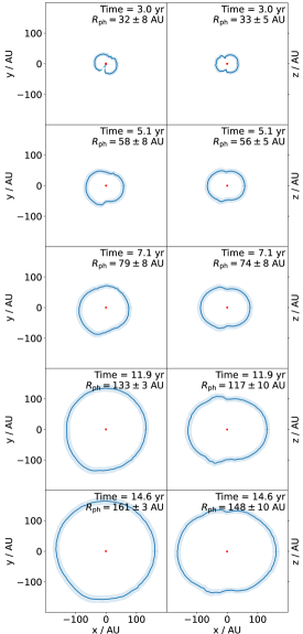
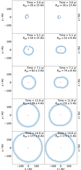
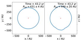
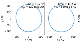
Figure 13: Photosphere cross section in the XY (1st and 3rd columns) and XZ plane (2nd and 4th columns) for 1.7 M_⊙ (left 2 columns) and 3.7 M_⊙ (right 2 columns) simulations. Blue lines mark the photosphere, the shaded area corresponds to the local smoothing length $h$, and the red dots are the point mass particles. The cross section is obtained by tracing 600 rays, coming out of the primary star and heading towards all directions in the observation plane, and locating the intersections (marked as blue dots) between these rays and the photosphere (i.e., where the optical depth $\tau$ reaches 1). The root mean square of the distance between these intersections and the primary star is marked as the photosphere radius, $R_{\rm ph}$. Note that the error on $R_{\rm ph}$ is the standard deviation of $R_{\rm ph}$ for each ray, and it is not the root mean square of $h$.

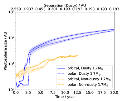
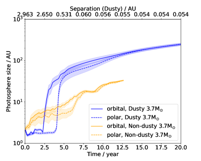
Figure 14: Photosphere size evolution in the orbital plane (solid line) and in the polar direction (dashed line) for the 1.7 M_⊙ (left panel) and the 3.7 M_⊙ (right panel) simulations with dust nucleation (blue lines) and without dust (orange lines). The orbital separation (for the simulations with dust) is marked on the top x-axis. The shaded area are the root mean square of the smoothing length interpolated at the intersection between the photosphere and the aforementioned directions, respectively.

Figure 13 shows the photospheric radius along the orbital and perpendicular planes for different moments in time. The radius is obtained by drawing 600 rays emanating from the AGB core point mass particle. The rays are evenly spaced from each other at equal angular intervals. The optical depth, $\tau$, is obtained at all locations on the rays, integrating inwards to give

$$\tau(\mathbf{r})=\int^{\infty}_{r}\kappa\rho\,d\mathbf{l},$$ (12)

where $\kappa$ is the opacity, $\rho$ is the density and the integration is over the ray of direction $d\mathbf{l}$. The density at a given position along the ray is computed using

$$\rho(\mathbf{r})=\sum_{j}m_{j}W(|\mathbf{r}-\mathbf{r}_{j}|,h_{j}),$$ (13)

where $m_{j}$ is the mass of particle $j$ and $W$ the smoothing kernel, which is a function of the position vector, $\mathbf{r}_{j}$, and of the particle’s smoothing length $h_{j}$. Thus

$$\tau=\sum_{j}\frac{\kappa_{j}m_{j}}{h_{j}^{2}}w_{\mathrm{col}}(q_{j}),$$ (14)

where, $\kappa_{j}$ is the particle’s opacity and $q_{j}$ is the dimensionless distance of the particle to the ray in units of $h_{j}$. The dimensionless column kernel, $w_{\mathrm{col}}(q_{j})$, is obtained by integrating the smoothing kernel $W(|\mathbf{r}-\mathbf{r}_{j}|,h_{j})$ along $d\mathbf{l}$

$$w_{\mathrm{col}}(q(x,y,z,h))=h^{2}\int W(\mathbf{r}(x,y,z),h)d\mathbf{l}.$$ (15)

The actual direction $d\mathbf{l}$ is not important since the smoothing kernel, $W$, is selected to be spherically symmetric. We use the cubic M₄ B-spline kernel from Schoenberg (1946) (see Monaghan 1992) as the smoothing kernel.

The particle’s opacity in the nucleation simulations is the sum of a constant gas opacity, $\kappa_{\mathrm{gas}}=2\times 10^{-4}\mathrm{cm}^{2}\mathrm{g}^{-1}$, and of the dust opacity, $\kappa_{\mathrm{d}}$, (as described by Eq. 7), giving

$$\kappa_{j}=\kappa_{\mathrm{gas}}+\kappa_{\mathrm{d},j}.$$ (16)

In the non-dusty simulations (Fig. 14), $\kappa_{j}=\kappa_{\mathrm{gas}}$ when the temperature $T<6000$ K, and $\kappa_{j}=0.2(1+X)=0.34\ \mathrm{cm}^{2}\mathrm{g}^{-1}$ otherwise (assuming a hydrogen mass fraction $X=0.7$). Hence, the optical depth contribution from particle $j$, $d\tau_{j}$, is

$$d\tau_{j}=\frac{\kappa_{j}m_{j}}{h_{j}^{2}}w_{\mathrm{col}}(q_{j}).$$ (17)

For each ray, particles that are within $2h_{j}$ from the ray where $w_{\mathrm{col}}(q_{j})$ is non-zero, are selected and arranged from closest to the observer to farthest, and the optical depth at any given particle’s projection on the ray (which is a line here) is then determined by summing the $d\tau$ from the observer to that particle $n$ via

$$\tau=\sum_{j=0}^{n}d\tau_{j}.$$ (18)

The photosphere is then found by interpolating the array of $\tau$ (at each particles’ projected location on the ray) to find the location where $\tau=1$. This is the location of the photosphere, marked as a blue line in Figures 13. At earlier time, the photosphere does not appear to enclose the central binary because dust formation has just started and the high opacity regions may only exist on one side of the binary. The absence of a dusty photosphere simply implies that at those times part of the photosphere is much closer to the binary, and the main source of opacity is the gas opacity at the boundary between ionised and recombined gas.

The smoothing length, $h$, at $\tau=1$ is represented as the light blue region in Figure 13 and gives an idea of the uncertainty on the photosphere’s location. It is calculated by finding the density using Eq. 13 at that location and calculating a corresponding value of $h$ using the relation

$$h=h_{\mathrm{fact}}\left(\frac{m}{\rho}\right)^{1/3},$$ (19)

(Price et al., 2018), where the dimensionless factor $h_{\mathrm{fact}}=1.2$, and the particle mass, $m$, is a constant for a given simulation.

This calculation clearly reveals the expansion of the photosphere over time and its morphological changes. As can be seen in the bottom panels in Figure 13, the photosphere grows from 130 to 160 to 430 au between 12, 15 and 43 years for the 1.7 M_⊙ model. The corresponding temperatures are 590 K, 490 K and 380 K, within about 10 per cent. For the 3.7 M_⊙ model the corresponding values are 140, 180, 530 au with temperatures of 1100 K, 500 K and 410 K. While the photosphere for both models starts with an equatorial enhancement, that of the 1.7 M_⊙ model remains so for longer while right at the end the prolate shape becomes mildly oblate. Not so for the 3.7 M_⊙ model which remains more spherical, likely because of the much smaller mass ratio. The radial velocity of the photosphere for the 1.7 M_⊙ model is 63, 62 and 57 km s^-1 at 12, 15 and 43 years, respectively, while for the 3.7 M_⊙ model it is 77, 80 and 72 km s^-1 at the same times.

Figure 14 shows the volume averaged radius of the photosphere in the orbital and polar direction, defined as the distance from the photosphere to the AGB core point mass particle. To calculate these values, four rays are averaged at each time step to measure the radius in the orbital plane ($\pm$x and $\pm$y) and two rays ($\pm$z) to measure the polar radius, where the radius along each ray is determined in the same way as in Figure 13. The average of the four or two measurements on the orbital plane is plotted as blue or orange lines in Figure 14, along with the average of the photospheric smoothing length, $h_{\mathrm{ph}}$, as an indication of the uncertainty (plotted as a light blue or orange shaded region). We note that in Figure 14 (left panel) the size of the photosphere at time zero for the 1.7 M_⊙ model is different between the dusty and non-dusty models. This is due to a slightly different initial model being used in the two simulations, where in the latter the star was relaxed in isolation for slightly longer and expanded to $\sim$2 au.

From Figure 14 we infer that, for the dusty models, the equatorial photosphere rapidly grows to a large size approximately one year before the polar photosphere, effectively indicating that there is a “hole" at the poles where an observer would see deeper into the object. However, this hole is filled rapidly and the size of the photosphere in the two orthogonal directions becomes very comparable, indicating an approximately spherical object as also seen in Figure 13. Interestingly, this is more so for the 3.7 M_⊙ models than for the 1.7 M_⊙ one. In the latter a slightly oblate shape is observed in the perpendicular cut until 14.6 yrs, but later in time, at 44 yrs, the shape has become clearly prolate. The effect of these relatively small departures from spherical symmetry on the light will be explored in a future work.

4 Discussion

4.1 Limitations of the current models

A major shortcoming of the current simulations is the absence of a proper treatment of radiative transfer which would allow to determine the dust temperature, localize the photosphere and have a better estimate of the radiative acceleration. Contrarily to our assumptions, the gas and dust temperatures are likely different and these differences will induce heat transfer from one component to the other, thereby introducing cooling/heating terms in the energy equations which are presently not accounted for. Since it has been shown (for details see Bowen 1988) that adiabatic simulations (that do not include cooling) of dust-driven AGB winds have a lower mass-loss rate than those simulations with radiative cooling (modelled using an isothermal equation of state), it is possible that including this physical mechanism leads to the gas reaching condensation temperatures in regions closer to the recombination of the ionized gas, and hence closer to the surface of the AGB star. This may have two effects: first, a larger dust nucleation rate (as dust seeds would form in denser regions), and consequently, a larger total dust mass growing at a faster rate. The second effect would be an increase in opacity in denser, slower regions of the envelope, with a greater radiation pressure on the dust, resulting in additional envelope expansion. In other words, radiative cooling could trigger a dust-driven outflow, similar to single AGB stars.

Our treatment of the radiative acceleration also assumes that the star keeps a constant luminosity and that photons are not absorbed until they reach the dust grains. Taking into account changes in the luminosity and photon absorption along the ray can impact the flow dynamics, the extent of which still needs to be assessed.

Another limitation is the lack of grain destruction mechanisms and the account of gas-to-dust velocity drift. In this regard, our simulations show that the densities in dust forming regions are sufficiently high for gas and dust to be dynamically coupled. On the other hand, our simulations showed that overdensities from spiral shocks provide sites for dust nucleation, but it remains to be confirmed that this effect persists when including dust destruction mechanisms.

We currently cannot calculate the nucleation and growth of oxygen-rich dust. As such we cannot consider the dust for low-mass AGB stars in stages prior to dredge-up episodes (i.e., with oxygen-rich envelopes), CE interactions with high mass giant stars undergoing hot bottom burning, which also have C/O $<1$, or massive red supergiants ($\gtrsim 10$ M_⊙). For this reason, we have only considered carbon dust with a C/O ratio that was chosen, somewhat arbitrarily, to be 2.5. Ventura et al. (2018) shows that stars with initial mass between 2 and 4 M_⊙, reach, by the end of the AGB, C/O values between 1.2 and 3.8. There is however quite a bit of disagreement between models, with “Monash” models (Karakas & Lugaro, 2016) showing that $\sim$4 M_⊙ stars (the exact mass depends on metallicity) do not end the AGB as carbon rich because hot bottom burning destroys carbon while producing nitrogen. On the other hand, 4 M_⊙ ATON models (Ventura et al., 2018) have, by the end of the AGB, large C/O ratios. In addition, many AGB stars would be caught into a CE before the end of the AGB evolution, so their C/O ratio would be lower. So in conclusion, it is difficult to say what C/O ratio should be used, or what is typical for the mass range investigated in this study. The value we have adopted is therefore reasonable. The effect of the exact C/O ratio on the results will be studied in future work.

4.2 Comparison with other models of dust production in CE interactions

In this paper we have presented the first self-consistent nucleation model for carbon dust in AGB stars involved in CE interactions. However, past work has already considered the possibility of dust in CEs and assessed its possible impact with a range of different methodologies.

Glanz & Perets (2018) determined the likely dust nucleation and dust driving properties of a CE between a 0.88 M_⊙, 90 R_⊙ RGB star and a companion. They used analytical models for dust nucleation in single stars, adopting the temperatures and densities from a non-dusty 3D hydrodynamic simulation. They concluded that the expanding common envelope should be able to form dust at 370 R_⊙, or 1.7 au and surmised that dust at this location may help boost the accelerations and aid in unbinding the envelope albeit over relatively long timescales ($\sim 10^{5}$ yr). We find on the contrary that dust forms at much farther radii, at 10-20 au (which is also the distance at which dust starts to form in the post-processed models of Iaconi et al. (2019), who, incidentally, use the same star as do Glanz & Perets (2018)). At the much shorter distance of 1.7 au from the core of the star, the temperature is always too high for dust formation. In fact when our models start dust formation, the companion is orbiting at approximately that distance ($\sim$2 au), which heats the gas and hence prevents dust from forming so close. We note that our stars are quite different from the one used by Glanz & Perets (2018), in that they have approximately twice and four times the mass and are on the AGB, instead of the RGB, and our star is 3-4 times larger. In addition, as we explained in Section 3, dust forms in already ejected gas, and does not contribute significantly to unbinding or additional acceleration.

MacLeod et al. (2022) appraised a number of observations of luminous red novae analysed and measured by Matsumoto & Metzger (2022) and surmised the radius of the dust photosphere at the time when the dust layer becomes opaque, as a function of the mass of the progenitor. To find the radius, they used the time it takes for the optical lightcurve to dim to 90 per cent of the maximum light, interpreted as the time span over which 90 per cent of the transient’s optical energy is radiated and known as $t_{90}$ in Matsumoto & Metzger (2022). To calculate the radius, MacLeod et al. (2022) multiplied $t_{90}$ by the velocity of the material obtained from Doppler-broadened emission lines. For their 2 and 4 M_⊙ cases, they find $r_{\rm 90}\sim 4$ and $\sim 10$ au, respectively. Our values, taken 5 yrs after the start of the simulation when the dust photosphere first appears, are 30-35 au and 15-20 au for the 1.7 and 3.7 M_⊙, respectively. Our estimates of $r_{\mathrm{90}}$ are somewhat larger for the 1.7 M_⊙ model, but quite similar for the 3.7 M_⊙ one. Our photospheric radius have an opposite dependence on the primary’s mass to what measured by MacLeod et al. (2022). This may be due to the mass ratio, which for the 3.7 M_⊙ model is much smaller (0.16) than for the 1.7 M_⊙ giant (0.35).

The amount of dust formed in our simulations ($0.8-2.2\times$10^-2 M_⊙) is similar to the most extreme case calculated by Lü et al. (2013). They calculated (oxygen) dust formation for common envelope interactions between stars with mass between 1 and 7 M_⊙ both at the base and at the top of the RGB, with a C/O number ratio equal to 0.4 (i.e., with mainly olivine- and pyroxene-type silicate dust grains) and with a 1 M_⊙ stellar companion. They used an a dust formation code and a 1D dynamical model of the expanding and cooling ejected CE. Only their RGB tip model with the steepest dependence between temperature and radius achieves a dust production similar to the dust mass produced by our models (which is close to the maximum possible).

4.3 Comparison between dust yields in CE interactions and in single AGB stars

Ventura et al. (2014) calculates that the amount of (carbon) dust formed in single AGB stars of 2 M_⊙ and Z=0.008 ranges between $10^{-4}$ and $10^{-3}$ M_⊙, depending on the mass-loss prescription, with masses as high as $10^{-2}$ M_⊙ for lower metallicities (Z=0.004). For a 2.5 M_⊙ star, they find a dust production ranging between $10^{-3}$ and $10^{-2}$ M_⊙. Their values are comparable but somewhat lower than ours ($0.8\times 10^{-2}$ and $2.2\times 10^{-2}$ M_⊙, for the 1.7 and 3.7 M_⊙ models, respectively), which can be explained by their different treatment of dust formation.

In our two simulations, carbon-rich AGB stars in a CE binary interaction deliver close to the maximum dust they can produce. This is somewhat contrary to the idea that the CE interrupts the AGB evolution, and incidentally its dust production. What our simulations show instead is that CE dramatically accelerates the production of dust, without altering significantly the amount of mass released.

4.4 Possible observational counterparts

Gruendl et al. (2008) detected a number of carbon stars in the Large Magellanic Cloud galaxy with very large infrared excesses, SiC in absorption, and an implied mass loss rate of 10^-4 M_⊙ yr^-1, about ten times larger than expected for single stars. These stars also point to low main sequence masses of 1.5-2.5 M_⊙. Galactic counterparts have similar properties, including similar mass-loss rates despite the higher metallicity of the Galaxy. CE ejections take place over a short time: the AGB envelopes of the 1.7 and 3.7 M_⊙ models have masses of $\sim$1.2 M_⊙ and $\sim$3.0 M_⊙, respectively and are ejected in approximately 20 yrs (Figure 2), giving mass loss rates of $\sim$10^-2–10^-1 M_⊙ yr^-1. Our simulations may not correctly mimic the immediate post-in-spiral timescale, and are unable to follow the system for the 2-3 centuries over which thermal relaxation may take place. During that time the mass-loss rate would decrease compared to the initial in-spiral values, but it is clear from the simulations that mass-loss rates would be substantially higher than for the inferred single star values. Taken together with the formation of $\sim$10^-2 M_⊙ of dust on very short timescale it makes the possibility that extreme carbon stars are caught in the aftermath of the CE in-spiral. Groenewegen & Sloan (2018) lists stars with L=5000-10 000 L_⊙ and effective temperatures of $\sim$300 K, which would imply photospheric radii between $\sim$100 and 200 au, not dissimilar to our inferred photospheric radii. It is not a stretch to consider these stars direct outcomes of CE interactions between low mass AGB stars and a companion.

In a similar way, water fountains have been proposed by Khouri et al. (2021) to be post-CE systems. Water fountain stars are oxygen-rich AGB stars, with H₂O maser emission related to fast polar outflows. They have optically thick, O-rich dusty envelopes, distributed in a torus shape, and are deduced to have extremely high mass-loss rates of $\sim 10^{-3}$ M_⊙ yr^-1, two orders of magnitude higher than the single star prediction. The water fountain phenomenon is estimated to last a few hundred years at most. These objects are compatible with the idea of a fast ejection of gas and dust, resulting in a transitional, but very optically thick dust shell. The seeming conflict between the equatorial dust tori in water fountain sources and the more spherical dust distribution in our simulations could be a result of the mass of the companion, where more massive companions likely result in more equatorially-enhanced dust distributions as seen in this study. The fast collimated outflows ensuing from the core are possibly magnetically collimated jets due to accretion of modest amounts of fall-back material onto the companion or core of the primary (assuming the binary has survived the common envelope). This type of fall-back and jet formation has been studied both observationally and theoretically by Tocknell et al. (2014) and Nordhaus & Blackman (2006) and the mechanisms are completely aligned with the idea that in water fountains we are observing the onset of the jets.

The expected high and fast dust production in CE evolution with AGB stars should leave some distinctive observational signatures in planetary nebulae, compared to nebulae deriving from single star and wider binary interactions. Planetary nebulae do not just form at the moment of the ejection of the AGB envelope (over tens of thousands of years as in single AGB stars or just decades as in common envelope interactions), but by the sweeping and ionising action of the stellar wind that follows the ejection. This may complicate the interpretation of the ejection history by studying the morphology, even in extreme cases, such as CE interactions.

Finally, there are many other possible CE ejections that are only now being discovered in the transient sky. An example are the “SPRITEs" (eSPecially Red Intermediate-luminosity Tansient Events; Kasliwal et al., 2017), that may be CE ejections involving more massive, red supergiants. These optically-invisible, mid-IR transients bear the hallmark of copious fast ejection of gas and dust. We leave it to future work to analyse these objects.

5 Conclusions

We have carried out two common envelope simulations with a 1.7 and a 3.7 M_⊙ AGB stars with a 0.6 M_⊙ companion, including a self consistent treatment of dust nucleation. We have used a C/O ratio of 2.5 (by number) to test not only the dust formation properties but also the wind-driving properties. Our main conclusions are:

1. In both simulations dust formation starts in a shell about 1 yr after the beginning of the simulation, well before the in-spiral phase takes place. At 5 years the dust forming shell is thin, has irregular thickness, and is located at $\approx 40$ au. For the 1.7 M_⊙ (3.7 M_⊙) simulation, this shells moves outward and by 20 years it reaches a distance of $\approx 160$ au (200 au) and is $\approx 40$ au (20 au) thick.

2. Dust formation starts in small grains to which monomers are added, increasing the dust grains size. As the dust grains move away from the seeds formation region, transported out by the expanding envelope, their size stops increasing. The dust that forms earlier ($\approx$2 years) remains smaller ($\approx$0.06 $\mu$m) than dust formed later (between 9 and 15 years; 0.4-0.6 $\mu$m).

3. The total dust mass is similar in the lower and higher mass simulations up to $\sim$22 years. At later times, the total dust mass is higher for the more massive envelope, eventually plateauing below the theoretical maximum, with total dust yields of $8.2\times 10^{-3}$ M_⊙ (1.7 M_⊙) and $2.2\times 10^{-2}$ M_⊙ (3.7 M_⊙). Therefore, the total mass of the dust formed depends to a greater extent on the metallicity and mass of the AGB envelope, other factors being of lesser relevance.

4. Dust formation does not lead to substantially more mass unbinding, although $\sim 10^{-2}$ M_⊙ of dust is produced. Dust forms too far in the wind to generate effective driving on a dynamical timescale required to aid with envelope ejection, because at those distances, the radiative flux is greatly diluted and gas is already unbound. It is possible — indeed likely — that given more time even small accelerations may build larger velocities.

5. Despite the lack of dust driving, the amount of dust that forms in the common envelope greatly impacts the optical appearance of the model. A simple calculation of the photospheric size of the models shows that at 12 years, where we compared the dusty and non-dusty models, the photosphere of the dusty model is $130$ and $140$ au, while for the non dusty model it is $20$ and $32$ au, for the 1.7 and 3.7 M_⊙ models, respectively, hence 4-7 times larger. At 15 years, the dusty simulations photospheres have grown to $160$ and $180$ au, and by 43 years they are $430$ and $530$ au, with an error of $\lesssim 10$ per cent. The corresponding mean temperatures at 12, 15 and 43 years are 590 K, 490 K and 380 K for the 1.7 M_⊙ model and 1100 K, 500 K and 410 K for the 3.7 M_⊙ model.

6. The morphology of the envelope in the presence of dust formation is nearly spherical. Initially the shape of the envelope is clearly elongated along the equatorial plane for both models. For the 1.7 M_⊙ model it remains somewhat elongated (oblate) to $\sim$15 yrs but by 44 yrs it becomes somewhat prolate. For the 3.7 M_⊙ model, which has a relatively lighter companion, the shape becomes nearly spherical by $\sim$15 years and remains so till the end of the simulation.

7. These simulations add further evidence to the suggestion that extreme carbon stars, water fountain stars, as well as some infrared transients might be objects caught in the immediate aftermath of a CE interaction on the AGB.

6 Data Availability

The data underlying this article will be shared on reasonable request to the corresponding author.

Appendix A Numerical consideration: the effects of resolution on dust formation and conservation properties of the simulations

The effect of resolution on parameters derived from phantom simulations of the common envelope interaction has been thoroughly investigated elsewhere (e.g., Iaconi et al., 2018; Reichardt et al., 2019, 2020; Lau et al., 2022; Gonzalez-Bolivar et al., 2022). The only quantities that have never been assessed are those connected to dust mass and dust growth.

Figure 15 displays the evolution of total dust mass with time for two CE simulations with a 3.7 M_⊙ AGB star, the simulation presented in this paper ($1.37\times 10^{6}$ SPH particles, black solid line) and one with identical stellar parameters but with only $2\times 10^{5}$ SPH particles (red dashed line in Figure 15). From Figure 15 it is evident that the amount of dust mass is very weakly dependent on resolution, and at the end of the simulations, the total amount of dust is the same. We therefore suggest that the simulated process of dust formation is nearly-independent of numerical resolution. While it would be appropriate to carry out a more canonical convergence test (at least three simulations differing in number of particles by a factor of at least 8, this is precluded by very long computation times).

At lower resolution the stellar structure used to carry out the simulation is not as stable as at high resolution. We have checked the stability and behaviour of the single stellar structure at low resolution by evolving it for 5 years in isolation, but with twice the softening length of the core (16 R_⊙). While we can confirm that the structure is not as stable, by 5 years only 3 per cent of the particles have expanded past the initial radius and the density profile is not overly distorted. Finally, no dust has formed in the isolated structure.

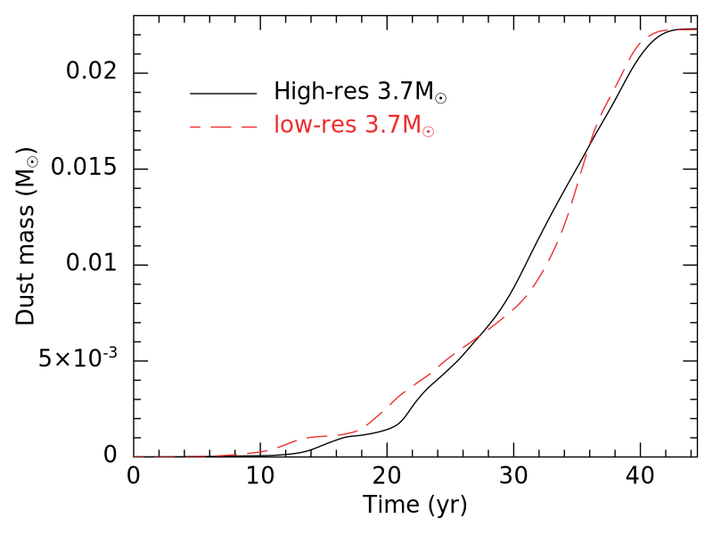
Figure 15: Dust mass as a function of time for the high-resolution production simulation presented in this paper ($1.37\times 10^{6}$ SPH particles, black solid line) and a low resolution ($2\times 10^{5}$ SPH particles, red dashed line) identical CE simulation with a 3.7 M_⊙ AGB star

In Figures 16 and 17 we evaluate the conservation and redistribution of energy and angular momentum in the dusty CE simulations. In the left panel the total energy (blue line) is conserved to within $1\%$. As the envelope expands the thermal energy decreases (red line), as does the potential energy of the cores that in-spiral towards one another (purple line). Every other energy (kinetic energy of the cores and gas (green line) potential energy of the envelope gas and cores (pink line) and potential energy of the gas (brown lines). (Note the orange line is the total potential energy, core-core, core-gas and gas-gas).

Energy conservation is achieved despite the fact that we inject energy in the form of radiative accelerations. The fact that the effect of the last term in Equation 10 is negligible is a result of the comparatively small accelerations that result from it, as explained in Section 3.2.

In the bottom panels of Figures 16 and 17 we plot the total angular momentum (blue line) that is conserved with an error of less than $1\%$. As the companion plunges into the primary’s envelope, the orbital angular momentum (red line) decreases and is transferred to the bound (yellow line) and unbound gas (green line). After 7 years, the inner gas region is almost in corotation, the gravitational drag force is considerably reduced, the separation stabilises and the orbital angular momentum becomes almost constant. From that moment there is no more angular momentum transfer from the point mass particles to the gas. The angular momentum of the bound material decreases as the amount of bound material is reduced due to thermal energy conversion into thermal energy and ultimately into work.

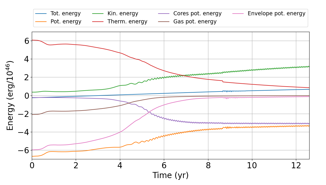
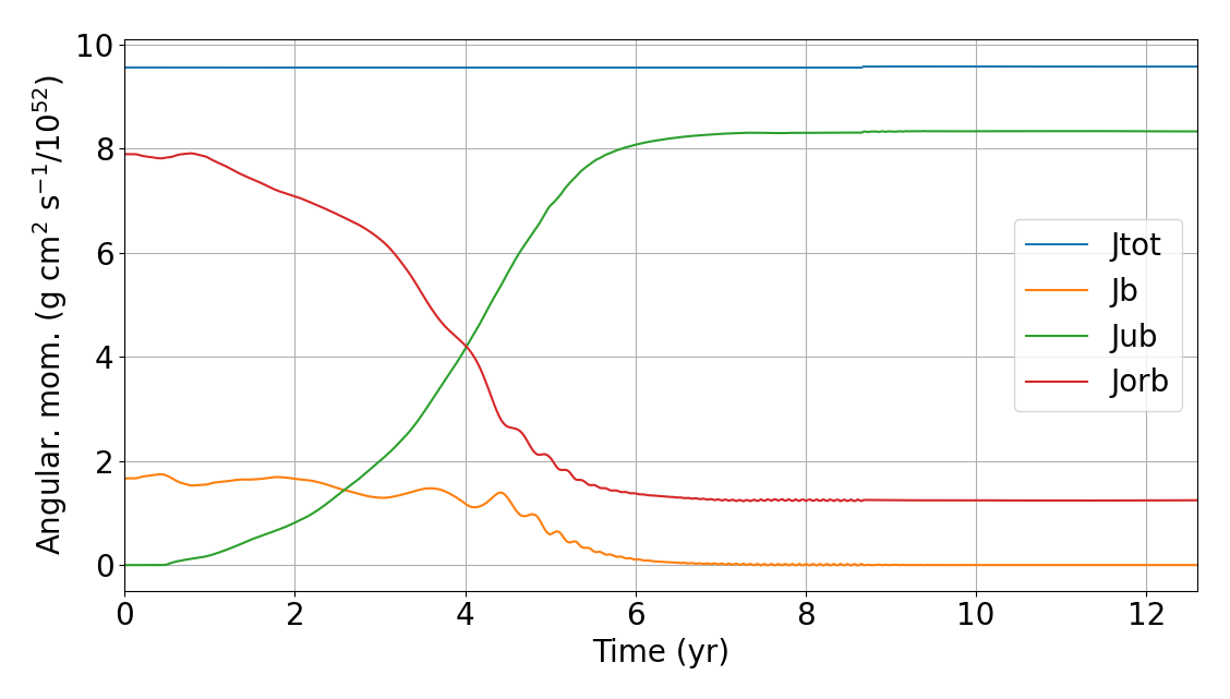
Figure 16: Energy (top panel) and angular momentum (bottom panel) evolution for the 1.7 M_⊙ simulation. Top panel: total energy (blue line), total potential energy (yellow line), kinetic energy (green line), thermal energy (red line), potential energy of the point mass particles (violet line), potential energy of the gas without point mass particles (brown line) and potential energy of the gas and point mass particles (pink line). Bottom panel: total angular momentum (blue line), orbital angular momentum (red line), angular momentum of the bound gas (yellow line) and of the unbound gas (green line).

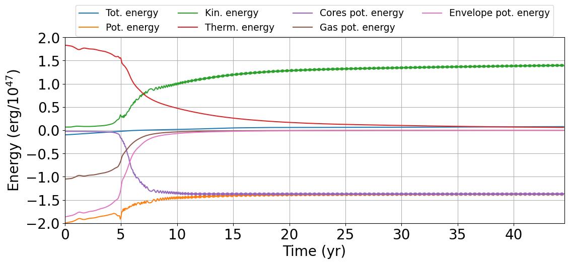
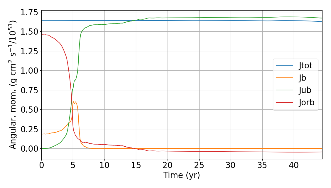
Figure 17: Energy (top panel) and angular momentum (bottom panel) evolution for the 3.7 M_⊙ simulation. Top panel: total energy (blue line), total potential energy (yellow line), kinetic energy (green line), thermal energy (red line), potential energy of the point mass particles (violet line), potential energy of the gas without point mass particles (brown line) and potential energy of the gas and point mass particles (pink line). Bottom panel: total angular momentum (blue line), orbital angular momentum (red line), angular momentum of the bound gas (yellow line) and of the unbound gas (green line).

References

- Bermúdez-Bustamante et al. (2020) Bermúdez-Bustamante L. C., García-Segura G., Steffen W., Sabin L., 2020, MNRAS, 493, 2606
- Blagorodnova et al. (2017) Blagorodnova N., et al., 2017, ApJ, 834, 107
- Bowen (1988) Bowen G., 1988, ApJ, 329, 299
- Chen et al. (2020) Chen Z., Ivanova N., Carroll-Nellenback J., 2020, ApJ, 892, 110
- De Marco & Izzard (2017) De Marco O., Izzard R. G., 2017, Publ. Astron. Soc. Australia, 34, e001
- Esseldeurs et al. (2023) Esseldeurs M., et al., 2023, arXiv e-prints, p. arXiv:2304.09786
- Gail & Sedlmayr (2013) Gail H.-P., Sedlmayr E., 2013, Physics and Chemistry of Circumstellar Dust Shells
- Gail et al. (1984) Gail H. P., Keller R., Sedlmayr E., 1984, A&A, 133, 320
- Glanz & Perets (2018) Glanz H., Perets H. B., 2018, MNRAS, 478, L12
- Gonzalez-Bolivar et al. (2022) Gonzalez-Bolivar M., De Marco O., Lau M. Y., Hirai R., Price D. J., 2022, arXiv preprint arXiv:2205.09749
- González-Bolívar et al. (2023) González-Bolívar M., Bermúdez-Bustamante L. C., De Marco O., Siess L., Price D. J., Kasliwal M., 2023, arXiv e-prints, p. arXiv:2306.16609
- Groenewegen & Sloan (2018) Groenewegen M. A. T., Sloan G. C., 2018, A&A, 609, A114
- Gruendl et al. (2008) Gruendl R. A., Chu Y. H., Seale J. P., Matsuura M., Speck A. K., Sloan G. C., Looney L. W., 2008, ApJ, 688, L9
- Iaconi et al. (2018) Iaconi R., De Marco O., Passy J.-C., Staff J., 2018, MNRAS, 477, 2349
- Iaconi et al. (2019) Iaconi R., Maeda K., De Marco O., Nozawa T., Reichardt T., 2019, MNRAS, 489, 3334
- Iaconi et al. (2020) Iaconi R., Maeda K., Nozawa T., De Marco O., Reichardt T., 2020, MNRAS, 497, 3166
- Ivanova et al. (2013) Ivanova N., et al., 2013, A&ARv, 21, 59
- Ivanova et al. (2015) Ivanova N., Justham S., Podsiadlowski P., 2015, MNRAS, 447, 2181
- Karakas & Lugaro (2016) Karakas A. I., Lugaro M., 2016, ApJ, 825, 26
- Kasliwal et al. (2011) Kasliwal M. M., Cenko S. B., Kulkarni S. R., Ofek E. O., Quimby R., Rau A., 2011, ApJ, 735, 94
- Kasliwal et al. (2017) Kasliwal M. M., et al., 2017, ApJ, 839, 88
- Khouri et al. (2021) Khouri T., Vlemmings W., Tafoya D., Pérez-Sánchez A. F., Sánchez Contreras C., Gómez J. F., Imai H., Sahai R., 2021, Nature Astronomy, p. arXiv:2112.09689
- Lau et al. (2022) Lau M. Y. M., Hirai R., González-Bolívar M., Price D. J., De Marco O., Mandel I., 2022, MNRAS, 512, 5462
- Lü et al. (2013) Lü G., Zhu C., Podsiadlowski P., 2013, ApJ, 768, 193
- MacLeod et al. (2022) MacLeod M., De K., Loeb A., 2022, ApJ, 937, 96
- Mathis et al. (1977) Mathis J. S., Rumpl W., Nordsieck K. H., 1977, ApJ, 217, 425
- Matsumoto & Metzger (2022) Matsumoto T., Metzger B. D., 2022, ApJ, 938, 5
- Monaghan (1992) Monaghan J. J., 1992, ARA&A, 30, 543
- Nicholls et al. (2013) Nicholls C. P., et al., 2013, MNRAS, 431, L33
- Nordhaus & Blackman (2006) Nordhaus J., Blackman E. G., 2006, MNRAS, 370, 2004
- Nozawa & Kozasa (2013) Nozawa T., Kozasa T., 2013, ApJ, 776, 24
- Paczyński (1971) Paczyński B., 1971, ARA&A, 9, 183
- Paxton et al. (2011) Paxton B., Bildsten L., Dotter A., Herwig F., Lesaffre P., Timmes F., 2011, ApJS, 192, 3
- Paxton et al. (2013) Paxton B., et al., 2013, The Astrophysical Journal Supplement Series, 208, 4
- Paxton et al. (2015) Paxton B., et al., 2015, ApJS, 220, 15
- Price et al. (2018) Price D. J., et al., 2018, Publ. Astron. Soc. Australia, 35, e031
- Reichardt et al. (2019) Reichardt T. A., De Marco O., Iaconi R., Tout C. A., Price D. J., 2019, MNRAS, 484, 631
- Reichardt et al. (2020) Reichardt T. A., De Marco O., Iaconi R., Chamandy L., Price D. J., 2020, MNRAS, 494, 5333
- Schoenberg (1946) Schoenberg I. J., 1946, Q. Appl. Math., 4, 45
- Siess et al. (2022) Siess L., Homan W., Toupin S., Price D. J., 2022, arXiv e-prints, p. arXiv:2208.13869
- Tocknell et al. (2014) Tocknell J., De Marco O., Wardle M., 2014, MNRAS, 439, 2014
- Tylenda et al. (2011) Tylenda R., et al., 2011, A&A, 528, A114
- Valsan et al. (2023) Valsan V., Borges S. V., Prust L., Chang P., 2023, MNRAS,
- Ventura et al. (2014) Ventura P., Dell’Agli F., Schneider R., Di Criscienzo M., Rossi C., La Franca F., Gallerani S., Valiante R., 2014, MNRAS, 439, 977
- Ventura et al. (2018) Ventura P., Karakas A., Dell’Agli F., García-Hernández D. A., Guzman-Ramirez L., 2018, MNRAS, 475, 2282