A Perturbed Value-Function-Based Interior-Point Method for Perturbed Pessimistic Bilevel Problems
Abstract
Bilevel optimizaiton serves as a powerful tool for many machine learning applications. Perturbed pessimistic bilevel problem PBP, with being an arbitrary positive number, is a variant of the bilevel problem to deal with the case where there are multiple solutions in the lower level problem. However, the provably convergent algorithms for PBP with a nonlinear lower level problem are lacking. To fill the gap, we consider in the paper the problem PBP with a nonlinear lower level problem. By introducing a log-barrier function to replace the inequality constraint associated with the value function of the lower level problem, and approximating this value function, an algorithm named Perturbed Value-Function-based Interior-point Method(PVFIM) is proposed. We present a stationary condition for PBP, which has not been given before, and we show that PVFIM can converge to a stationary point of PBP. Finally, experiments are presented to verify the theoretical results and to show the application of the algorithm to GAN.
keywords:
Bilevel optimization , perturbed pessimistic bilevel problem , Perturbed Value-Function-based Interior-point Method(PVFIM) , stationary point.[1]organization=School of Mathematical Sciences,addressline=Dalian University of Technology, city=Dalian, country=China \affiliation[2]organization=DUT-RU International School of Information Science and Engineering,addressline=Dalian University of Technology, city=Dalian, country=China
[3]organization=School of Mathematical Sciences,addressline=Dalian University of Technology, city=Dalian, country=China
1 Introduction
Bilevel optimization has received significant attention in many machine learning applications including hyperparameter optimization[6, 8, 19, 20, 23], meta learning[7], neural architecture search[14], and Generative Adversarial Networks(GAN)[9, 21]. Mathematically, bilevel optimization can be described as follows:
| (1) | ||||
where , is a set dependent on , , are the objective functions of the lower level(LL) problem and upper level(UL) problem, respectively, and for each , the feasible region of is , which consists of optimal solutions to the LL problem. Moreover, as the bilevel problem can be can be thought of as a two-player game, the LL problem and the UL problem also can be called the follower and the leader, respectively; see [10, 15].
However, the goal of the bilevel problem in (1) is ambiguous if set is not singleon for some , since the minimization in the UL problem is only with respect to(w.r.t.) . To resolve it, (1) is usually reformulated into the optimistic bilevel problem or the pessimistic bilevel problem depending on practical applications[15, 3, 27, 12]. To be concrete, if the LL and UL problems are cooperative[27], problem (1) is generally reformulated into the optimistic bilevel problem:
If, on the other hand, the LL and UL problems are uncooperative[27], problem (1) is generally reformulated into the pessimistic bilevel problem(PBP):
| (2) |
Since the optimistic bilevel problem is easier to address, optimality conditions and numerical algorithms have been extensively studied; e.g., [10, 3, 27, 26, 11, 25]. In contrast, there are few algorithms available for the pessimistic bilevel problem.
Recently, for pessimistic bilevel problems with optimal solutions, some algorithms have been developed. Specifically, a penalty method, a reducibility method, a Kth-Best algorithm, and a descent algorithm are proposed in [1], [30], [29], and [4], respectively, to compute global or local optimal solutions for linear pessimistic bilevel problems with optimal solutions. In addition, for the general pessimistic bilevel problems with optimal solutions, a maximum entropy approach, a Relaxation-and-Correction scheme, and an algorithm named BVFSM are proposed in [31], [28], and [17], respectively, to compute global optimal solutions.
However, as is known, the optimal solutions to pessimistic bilevel problems can not be guaranteed to exist generally due to the very strong assumptions for ensuring the existence of optimal solutions[12]. In this sense, it seems that problem (2) is not well defined. To address the problem, researchers have proposed to replace the PBP in (2) with another solvable approximation problem[12, 18]. As done in [12, 18], replacing the optimal point set in (2) with the set of -optimal points , where is an arbitrary positive number and , a perturbed pessimistic bilevel problem PBP:
| (3) |
can be obtained. It is proved in [12] that under certain mild assumptions, PBP is solvable for any , and that the minimum value of PBP can approximate the infimum of PBP in (2) arbitrarily well as long as we choose sufficiently small . Actually, problem PBP is itself a meaningful problem. For example, the leader may only want to execute a decision that performs best among all -optimal solutions. After all, it is generally difficult to obtain a globally optimal solution to the LL problem.
Therefore, in this paper, we reformulate problem (1) where the leader and the follower are uncooperative as the problem PBP in (3) following [12, 18], and consider problem PBP. As far as we know, the convergence of the existing algorithms for PBP can be guaranteed only when the lower level problem is linear. Recently, for problem PBP with the linear lower level problem, [12] showed the equivalence between PBP and a single-level mathematical program MPCC regarding global optimal solutions, and a mixed integer approach is proposed to solve MPCC to obtain the global optimal solution of PBP. [28] mentioned that the Relaxation-and-Correction scheme for solving PBP can be used to solve problem PBP to obtain global optimal solutions. However, the Relaxation-and-Correction scheme is only used to solve the linear pessimistic bilevel problem, and the algorithms for solving general pessimistic bilevel problems are not provided.
In the paper, our aim is to develop a provably convergent algorithm for PBP in (3) with nonlinear lower level problem. Firstly, we obtain the stationary condition of PBP by using the standard version of PBP proposed in [12], the value function approach, and the Fritz-John type necessary optimality condition, as usally done for optimistic bilevel problems. Then, motivated by the recent work in [17] for solving pessimistic bilevel problems, we propose an algorithm named Perturbed Value-Function-based Interior-point Method(PVFIM). To be specific, we first reformulate PBP as a problem containing an inequality constraint. Later, we introduce a log-barrier term into the UL function to remove the inequality constraint, and use an approximate function to replace the resultant objective function. As a result, by solving a sequence of approximate minimax problems, we can obtain the solution of PBP. Theoretically, we show that PVFIM can produce a sequence from which we can obtain a stationary point of PBP. Our main contributions are listed below:
-
(1)
We present a stationary condition of problem PBP, which has not been given before.
-
(2)
We develop an algorithm named PVFIM for problem PBP with nonlinear lower level problem, and we prove that PVFIM can converge to a stationary point of PBP; we are the first to provide the provably convergent algorithms for PBP with nonlinear lower level problem.
-
(3)
We perform experiments to validate our theoretical results and show the potential of our proposed algorithm for GAN applications.
For the rest of this paper, we first make some settings for problem PBP in (3), and review some materials on nonsmooth analysis in Section 2. Next, we propose a new algorithm named PVFIM for problem PBP in Section 3. Then, in Section 4, we show the convergence of our proposed algorithm. Finally, we present the experimental results in Section 5, and conclude and summarize the paper in Section 6.
Notations. We denote by the norm for vectors and spectral norm for matrices. We use to denote the open ball centered at with radius , and for a set , co denotes the convex hull of . For , denotes the gradient of taken w.r.t. , (resp. ) denotes the gradient of (resp. ) w.r.t. (resp. ), and and .
2 Preliminaries
In this section, we first make some settings for problem PBP in (3). Then we review some background materials on nonsmooth analysis.
2.1 Problem Setting
In this paper, for PBP in (3), we set to be a fixed set for , that is, for any given , we consider problem PBP below:
| (4) |
where , and
| (5) |
In the following, we first make some assumptions on the constraint sets.
Assumption 1.
We suppose that sets and are nonempty, convex, and closed. Furthermore, there exist positive numbers and such that
for all and .
Next, we make some assumptions on the objective functions.
Assumption 2.
We suppose that is a set containing , open, and convex; functions , are twice continuously differentiable. Furthermore, for each , is -strongly concave on ; is convex on .
Based on Assumption 1 and Assumption 2, the differentiability of in (5) can be ensured, as shown below.
Proposition 1.
For the proof of Proposition 1, you can refer to Proposition 1 in [11]. In the following, some Lipschitz conditions are imposed on the objective functions.
Assumption 3.
Let , .
-
(1)
and are - and -Lipschitz, respectively, that is, for any , , , ,
-
(2)
and are - and -Lipschitz, respectively, that is, for any , , , ,
-
(3)
and are - and -Lipschitz, respectively, that is, for any , , , ,
To facilitate our further discussion, we provide the definitions of local optimal solutions and interior points below.
Definition 1.
A point is called a local optimal solution for problem PBP in (4), if there exists a neighbourhood of such that
Definition 2.
Given a set , a point is called an interior point of , if there exists a such that .
Furthermore, to obtain a stationary condition of PBP, the following assumption is made.
Assumption 4.
All the local optimal solutions for problem PBP in (4) are in the interior of .
We remark that Assumption 4 is mild. In the following, an example which satisfies Assumption 4 is shown.
Example 1.
For problem PBP in (4), let and . It is obvious that the local optimal solutions of on are , and , and all of them are the interior points of .
2.2 Basic Tools
For the nonsmooth function , and denote the limiting subgradient and the Clarke generalized gradient of at , respectively.
In the following proposition, we borrow the conclusions on the Clarke normal cone and the Clarke generalized gradient which are given in [24] and (2.5), (2.6) of [5].
Proposition 2.
-
(1)
If is a nonempty, closed, and convex set, then the Clarke normal cone to at , i.e., , can be expressed as follows:
-
(2)
If function is Lipschitz continuous near , then . Furthermore, .
Next, following Corollary 2.4.2 in [22], we show the following calculation rule for the Clarke generalized gradient which is useful in the paper.
Proposition 3.
Suppose is Lipschitz continuous near , and is continuously differentiable near . Then
Then, we consider the following optimization problem:
| (6) | ||||
where
| (7) |
Notice that in (7) is generally nonsmooth even if functions and are smooth. Therefore, problem (2.2) is generally a nonsmooth optimization problem. Recently, [26] showed that if all the functions involved for a nonsmooth optimization problem are local Lipschitz continuous, the generalized lagrange multiplier rule of Clarke can be used to obtain the necessary optimality condition of the nonsmooth optimization problem.
To go further, the following assumption for problem (2.2) is made.
Assumption 5.
Let and be nonempty, convex, and compact. For any , suppose is Lipschitz continuous near , and , , are continuously differentiable functions.
It is obvious that Assumption 5 can imply that , , and are local Lipschitz continuous on . In the following, a sufficient condition for the local Lipschitz continuity of in (7) is provided.
As preparation, for each , we define
| (8) |
Furthermore, given , for satisfying and , we define
| (9) |
where , and the definition of is given in Proposition 2.
Proposition 4.
Suppose Assumption 5 holds. Let be an interior point of . Define
where the definitions of and are given in (8) and (2.2) with and , respectively. If , then in (7) is Lipschitz continuous near , and the limiting subgradient of at satisfies
where the definitions of and are given in (8) and (2.2) with and , respectively.
3 Algorithm
The structure of problem PBP in (4) is intricate. It involves three intricated optimization problems. To obtain a problem easier to tackle, the existing studies [12, 28] for problem PBP focus on reformulating PBP into a single level mathematical program MPCC based on the KKT condition. However, problem PBP and MPCC are only equivalent in the sense of global optimal solutions. Thus, they need to solve MPCC to global optimum to obtain a solution of PBP. Unfortunately, MPCC is still hard to solve, and the solution procedure for MPCC to obtain the global optimal solutions is not practical for machine learning applications since there are many constraints for the MPCC.
In the paper, we propose a new approach for PBP, i.e., reformulating PBP into a two level approximate minimax problem, and solving a sequence of approximate minimax problem to obtain the solution of PBP.
3.1 Approximate Minimax Problem
Given , recall that in (4) is the value function of the following optimization problem:
| (10) |
where , and is defined in (5).
By using the definition of , problem (10) can be written as
Then, motivated by the recent work in [17] for solving problem PBP, a log-barrier term is introduced into the objective function to remove the inequality constraint, and the following problem
| (11) |
where , is obtained.
It is obvious that in (11) is an implicitly defined function. To obtain the value of , we need to solve problem
| (12) |
to global optimality, which is impractical. In order to deal with the problem, we replace in (11) with
| (13) |
where , an approximate solution to problem (12), is obtained by running steps of projected gradient descent starting from initial value in the form of
| (14) |
with , where is the stepsize.
As a result, we approximate PBP in (4) by the minimax problem
| (15) |
where , is a positive integer,
| (16) |
and the definition of is given in (13).
To go further, the following assumption is made on the projected gradient descent steps for solving problem (12).
Assumption 6.
We remark that Assumption 6 is mild. In the following, an example which satisfies Assumption 6 is shown.
Example 2.
Under Assumptions 2 and 6, in (13) can be ensured to be differentiable(see Lemma 4 in the appendices). Then, for the minimax problem in (15), we define the first order Nash equilibrium point as follows.
Definition 3.
We say that a point , which satisfies , , and , is a -first order Nash equilibrium(-FNE) point of problem (15) if satisfies
Furthermore, recall that for each , in (15) is the value function of maximization problem:
| (18) |
where is given in (16). In the following, an assumption on the maximization problem in (18) is made.
Assumption 7.
Remark 1.
Under Assumptions 1, 2, and 7, for any positive integer , the set defined in (19) is nonempty, compact, and convex. To be specific, let be any given positive integer. From Assumption 7, we know that is nonempty since for any , , at least a global optimal solution to problem (18) with , , is in the set ; from Assumption 1, we know that is bounded; from Assumption 2, we know that is continuous and convex w.r.t. , and therefore, is closed and convex. Therefore, is nonempty, compact, and convex.
In the following, an example which satisfies Assumption 7 is shown.
Example 3.
For problem PBP in (4), we let , , , , where . Following the above discussion, PBP can be approximated by the minimax problem in (15), and the corresponding maximization problem is in (18). Setting . It is easy to know that for any , positive integer , we have , which can be obtained by using the definition of in Proposition 1 and the definition of in (13). As a result, for any positive integer , we have
where is defined in (19) with . Furthermore, by simple calculations, it is easy to know that , and for any , positive integer , , the global optimal solution to problem (18) is , which belongs to the set , and thus belongs to the set . Therefore, Assumption 7 is satisfied by setting .
Next, for any , positive integer , , we consider the following optimization problem
| (20) |
where
| (21) |
, and is a sufficient small number. Notice that if Assumption 7 holds, and we set ( in Assumption 7), the optimal solution to problem (20) must be an optimal solution to problem (18) since for the defined in (19), we have . Thus, we can obtain an approximate solution to problem (18) by solving problem (20). To facilicate our theoretical analysis, in the following, instead of solving problem (18) directly, we solve problem (20) to obtain an approximate solution to problem (18).
3.2 A New Algorithm Named PVFIM for Problem PBP in (4)
Based on the above discussion, a new algorithm named PVFIM is proposed for problem PBP in (4), as shown in Algorithm 1. For the minimax problem in (15), by setting , , a -FNE point can be obtained(see line 2 in Algorithm 1). By varying the values of , , , it produces a sequence of approximate first order Nash equilibrium points , from which we can obtain a stationary point of problem PBP.
We next illustrate how to obtain a -FNE point for problem (15) with , . As shown in Algorithm 2, for each , it first runs steps of projected gradient descent starting from initial value in the form of (14) to obtain an approximate solution to problem (12) with (see line 4 in Algorithm 2), and thus obtain the value of (see line 6 in Algorithm 2). Then by setting the projected region to be (see line 7 in Algorithm 2), it runs steps of projected gradient ascent to obtain an approximate solution to problem (20), and thus obtain an approximate solution to the maximization problem of problem (15) with (see line 10 in Algorithm 2). Based on the output in line 4 of Algorithm 2 and the output in line 10 of Algorithm 2, it constructs
| (22) |
with as an estimate of the gradient .
4 Theoretical Results
In the section, we first present the stationary condition for problem PBP in (4). Then, we prove that PVFIM can converge to the stationary point of problem PBP. Detailed theoretical analysis can be found in the appendices.
4.1 Stationary Condition for Problem PBP in (4)
Recently, the necessary optimality conditions[5] for PBP are derived. It is naturally to think of utilizing the necessary optimality conditions of PBP to obtain the stationary condition of PBP since PBP is a variant of PBP. However, the necessary optimality conditions for PBP are obtained under additional Lipschitz conditions, which are very strong and would limit the application scope of the algorithm. To deal with the problem, we use the standard version of PBP, the value function approach, and the Fritz-John type necessary optimality condition to obtain the stationary condition of PBP.
| (23) |
where
| (24) |
The relation between local optimal points of PBP and SPBP can be established as follows; see Proposition 4.2 in [12].
Proposition 5 ([12]).
Proposition 5 shows that problem PBP in (4) and problem SPBP in (23) are equivalent in terms of local optimal solutions if is a single point set for any . Notice that by using the value function approach [3, 27, 26], SPBP in (23) can be written as the following single level mathematical programming problem, denoted as SPBP still,
| (25) | ||||
with the help of function
| (26) |
and the definition of .
Proposition 6.
Proposition 6 can be easily obtained following Remark 3.1 in [10]. By combining Proposition 5 and Proposition 6, we know that, if is a local optimal solution to problem PBP in (4), then is a local optimal solution to problem SPBP in (4.1) for any . Thus, the stationary condition for problem PBP can be obtained by using the necessary optimality condition of problem SPBP in (4.1).
In the following, a Fritz-John type necessary optimality(FJ) condition for problem SPBP in (4.1) is shown, which is obtained based on the nonsmooth analytical material introduced in Section 2.
Theorem 2 (FJ condition).
Suppose Assumptions 1 and 2 hold. Let be a local optimal solution to problem SPBP in (4.1), with being an interior point of . Then there exist , , and not all zero, inteters , , satisfying , , , where , , and the definition of is given in (24), such that
and for each , ,
where for , , can be computed through Proposition 1, and the definition of is given in Proposition 2.
In the following, we show that for any feasible point of problem SPBP in (4.1), with being an interior point of , the above FJ condition with can be satisfied.
Proposition 7.
Nevertheless, the FJ condition for problem SPBP is a weaker optimality condition. However, the assumption for the KKT condition(i.e., the FJ condition in Theorem 2 with ) in [26] is very strong, which would limit the application of the algorithms. Therefore, we still use the FJ condition in the paper. In fact, our proposed algorithm can converge to a point which satisfies the FJ condition in Theorem 2 with .
4.2 Convergence of PVFIM in Algorithm 1
In this subsection, we show the convergence of PVFIM in Algorithm 1. Firstly, we show that for any given , Algorithm 2 can find a -FNE point for problem (15) in which is an arbitrary positive integer, and satisfies the inequality in (27) if we choose , to be the numbers that satisfy the inequalities in (28).
Theorem 3.
Suppose Assumptions 1, 2, 3, 4, 6, and 7 hold. Let in Algorithm 1 be the number equal to in Assumption 7. Assume that for any , positive integer , ,
is an interior point of , where is given in (16), and is given in (21) with . Let . Given , for problem (15), let be an arbitrary positive integer, and be a positive number satisfying
| (27) |
where
, , and , , , and are given in Assumptions 1, 3, 3, and 7, respectively, and , , are given in Lemmas 5, 6, and 7 in the appendices, respectively. Choose stepsizes , , in Algorithm 2 to be , , and , where is given in Assumption 3. Then if
| (28) |
where is given in Lemma 8 in the appendices, and and are given in Assumptions 1 and 2, respectively, Algorithm 2 can find a -FNE point for problem (15), that is, there exists such that is a -FNE point of problem (15).
Theorem 4.
Under the same conditions of Theorem 3. Let , , in Algorithm 1 be the sequences such that , , and for each positive integer , , is the number satisfying (27) with , , , are the numbers satisfying the inequalities in (28) with and , stepsizes , , are chosen according to Theorem 3 with , and be the -FNE point generated by Algorithm 2 for solving problem (15) with , . Then if is an accumulation point of the sequence with being an interior point of , is a stationary point of problem PBP in (4).
We remark that there must exist accumulation points for the sequence by the compactness of sets and , and the -component of the accumulation points can be guaranteed to be in the interior of if is a sufficient large region. Furthermore, let be a positive integer, for each positive integer , let , , , , and , where
with and , and , , , , , , are the numbers same to that given in Theorem 3. By simple calculations, it is easy to know the sequences , , , , satisfy the condition in Theorem 4 by choosing appropriate .
5 Experimental Results
We first validate the theoretical results on a synthetic perturbed pessimistic bilevel problem. Then we evaluate the performance of our proposed algorithm PVFIM on the applications to GAN.
5.1 Synthetic Perturbed Pessimistic Bilevel Problems
In this subsection, we perform experiments on the perturbed pessimistic bilevel problem PBP in (4) whose constraint sets and objective functions are given in Example 3. The experimental details are in the appendices.
By simple calculations, it is easy to know that this perturbed pessimistic bilevel problem PBP satisfies all the conditions in Theorem 4.
Following the discussion in Section 4, PBP can be reformulated as the problem SPBP in (4.1). By simple calculations, for each , ( is given in (24)), which is a single point set, and thus problem PBP and problem SPBP in (4.1) are equivalent in terms of local optimal solutions(see Propositions 5, 6). Furthermore, the feasible points to problem SPBP in (4.1) are with , , and the local optimal points to problem SPBP in (4.1) are with , , , and with , , , which are also global optimal points.
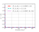
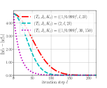
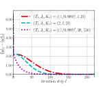
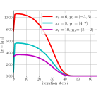
In Figure 1, we set the initial point to be , , and evaluate the performance of PVFIM with different choices of for each positive . It shows that, for all the cases, PVFIM can converge to the optimal point of problem SPBP in (4.1), which naturally implies that PVFIM can converge to the optimal point of problem PBP. Notice that and do not follow the condition in Theorem 4, and under the case that , PVFIM converges fastest among all the cases. Therefore, Figure 1 shows that in practice, does not have to follow the condition in Theorem 4, and choosing the appropriate can accelerate the convergence of PVFIM.
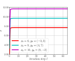
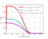
In Figure 2, we choose different initial points to evaluate the performance of PVFIM. It shows that PVFIM always can converge to a feasible point, whose -component is an interior point of , of problem SPBP in (4.1), and thus PVFIM always can converge to a stationary point of problem PBP(see Proposition 7).
5.2 Generative Adversarial Networks
In this subsection, we perform experiments on GAN to illustrate the applications of PVFIM for solving perturbed pessimistic bilevel problems. GAN generates samples from a data distribution by gaming, in which two models, i.e., a generator generating data, and a discriminator classifying the data as real or generated, are involved[9]. The training objective for the discriminator is to correctly classify samples, while the training objective for the generator is to make the discriminator misclassify samples. The training objective of GAN can be expressed as the bilevel problem in (1)[16] in which
and
where denotes the parameters of the generator , denotes the parameters of the discriminator , is the real data distribution, is the model generator distribution to be learned, is the data generated by the generator, is the coefficient of the regular term introduced to ensure the strong concavity of w.r.t. , and is introduced to ensure the fully convexity of w.r.t. . Notice that for the discriminator, only the parameters of the last linear layer are updated.
At present, there are mainly two methods to train GAN. The first method to train GAN is to perform gradient descent on and ascent on from the perspective of minimax optimization, which is done in the original GAN[9]. While the second method to train GAN, done in unrolled GAN[21], is based on the unrolled optimizaiton to update from the perspective of bilevel optimization. However, the convergence of the unrolled optimization methods for bilevel problems can be guaranteed only in the case where the solution to the LL problem is unique.
If considering GAN from the perspective of bilevel optimizaiton, we think that it would be suitable to reformulate the bilevel problem corresponding to GAN as the perturbed pessimistic bilevel problem in (4) to deal with the case where there are multiple solutions in the LL problem, since the objectives of the generator and the discriminator are adversary. Therefore, PVFIM provides a method to train GAN.
In the following, we compare GAN, unrolled GAN, with our proposed method on different datasets. The experimental details are in the appendices.
Please note that in practie, the parameters and are located in bounded sets. Thus, the fesible regions of and can be considered to be large regions, and the projected operations in lines 4, 12 of Algorithm 2 can be ignored automatically. Furthermore, the projected operations in line 10 of Algorithm 2 can be ignored automatically if we choose in Algorithm 1 to be a sufficiently small number.
5.2.1 Synthetic Data
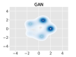
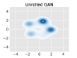
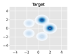
We first evaluate the performance of our method PVFIM on a synthesized 2D dataset following [21]. The real data distribution is a mixture of 5 Gaussians with standard deviation 0.02, and the probability of sampling points from each of the modes is 0.35, 0.35, 0.1, 0.1, and 0.1, respectively. The target samples are drawn from the real data distribution and the number of target samples is 512.
| GAN | Unrolled GAN | PVFIM | |
| Wasserstein distance | 0.452 | 0.346 | 0.299 |
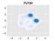
From Figure 3 and Table 1, we observe that PVFIM can generate samples which has the smallest Wasserstein distance to the target samples, which shows the validality of PVFIM on the application to GAN with synthetic data. Furthermore, since PVFIM can be used to solve the bilevel problem with multiple solutions in the lower level problem, it obtains better performance than unrolled GAN in the experiments.
5.2.2 Real-World Data
We then perform experiments on two real-world datasets: MNIST[13] and CIFAR10, to evaluate the performance of PVFIM. The MNIST dataset consists of labeled images of grayscale digits, and the CIFAR10 dataset is a natural scene dataset of . Inception Score(IS) is employed to evaluate the quality and diversity of the generated images, and the Frechet Inception Distance score(FID) is used for measuring the Frechet distance between the real and generated data distributions.
| Method | MNIST | CIFAR10 | ||
|---|---|---|---|---|
| IS | FID | IS | FID | |
| GAN | 6.05 | 189 | 2.89 | 241 |
| Unrolled GAN | 4.60 | 250 | 2.88 | 264 |
| PVFIM | 6.32 | 181 | 2.90 | 223 |
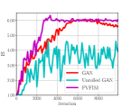
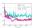
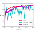
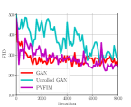
Figure 4 and Table 2 show that PVFIM can obtain the lowest FID and highest IS on both MNIST and CIFAR10 datasets, which shows the validality of PVFIM on the application to GAN with real-world data. Furthermore, since PVFIM can be used to solve the bilevel problem with multiple solutions in the lower level problem, it obtains better performance than unrolled GAN in the experiments.
6 Conclusion
In the paper, we provide the first provably convergent algorithm for the perturbed pessimistic bilevel problem PBP with nonlinear lower level problem, and we provide a stationary condition for problem PBP, which has not been given before. Moreover, the experiments are presented to validate the theoretical results and show the potential of our proposed algorithm in the applications to GAN.
Acknowledgments
The work is partially supported by the National Key R&D Program of China (2018AAA0100300 and 2020YFB1313503), National Natural Science Foundation of China(Nos. 61922019, 61733002, 61672125, and 61976041), and LiaoNing Revitalization Talents Program(XLYC1807088).
Appendix A Proof of Theorem 2 and Proposition 7
In this section, we first obtain a Fritz-John type necessary optimality condition for problem SPBP in (4.1).
It needs to remark that although , , and are differentiable under Assumptions 1 and 2, where the differentiability of can be obtained from Proposition 1, defined in (26) is generally nonsmooth. As a result, problem SPBP in (4.1) is a nonsmooth problem in general. Recall that if is local Lipschitz continuous, a Fritz-John type necessary optimality condition for SPBP in (4.1) can be obtained following from Theorem 1. For more details, see the nonsmooth analysis material given in the main text.
In the following, we first investigate the local Lipschitz continuity of . Notice that by using the definition of in (10), in (26) can be equivalently converted into
| (29) |
Similar to the discussion in the nonsmooth analysis material of the main text, given , for satisfying , , we define
| (30) |
where , and the definition of is given in Proposition 2. Then a sufficient condition for the local Lipschitz continuity of is shown below.
Lemma 1.
Suppose Assumptions 1 and 2 hold. For problem SPBP in (4.1), if is an interior point of , then in (26) is Lipschitz continuous near , and the Clarke generalized gradient of at satisfies
where
with the definitions of and given in (24) and (A) with and , respectively, and can be computed through Proposition 1.
Proof 1.
We first prove the Lipschitz continuity of near , which further implies the Lipschitz continuity of near . To start with, we define
| (31) |
Notice that is an interior point of . From Proposition 4, we know that the Lipschitz continuity of near can be guaranteed if for all , where the definition of is given in (A) with and .
Then, in the following, we prove that for all . Recall that for any ,
Assume that there exists such that
Then, we must have
| (32) |
and
| (33) |
From (32) and the definition of in Proposition 2, we know that , , which further implies that since is convex on (see Assumption 2). Therefore, we have by the definition of in (5). However, it contradicts with the formula in (33), since is a positive number. Therefore, for all . As a result, both and are Lipschitz continuous near .
Next, we consider the Clarke generalized gradient of at , i.e., .
Recall that . From Proposition 2, we know that
| (34) |
Since is an interior point of , and for all , from Proposition 4, satisfies
where the definitions of and are given in (A) and (31) with and , respectively, and can be computed via Proposition 1.
Furthermore, by the definition of and the fact that , we know that . Combined with (34), that can be obtained. Then, the proof is complete.
A.1 Proof of Theorem 2
In the following, the proof of Theorem 2 is shown.
Proof 2.
Firstly, since is an interior point of , from Lemma 1, we know that in (26) is Lipschitz continuous near , and the Clarke generalized gradient satisfies , i.e., there exist positive integers , , satisfying , , with given in (A) with , , where , , such that
| (35) |
where we use the definition of given in Lemma 1 and the definition of convex hull.
Then, since is a local optimal solution to problem SPBP in (4.1), from Theorem 1, we know that there exist , , not all zero such that
| (36) | ||||
where is given in (35), can be computed through Proposition 1, the definition of is given in Proposition 2, and we use the fact that since is an interior point of .
A.2 Proof of Proposition 7
In the following, the proof of Proposition 7 is shown.
Proof 3.
Since is a feasible point of problem SPBP in (4.1), we know that satisfies the following constraints:
| (37) |
Moreover, by the definition of in (26), it is easy to know that for any , satisfying , we always have
| (38) |
Combining (37) with (38), we know that , i.e., . Therefore, is the global optimal solution of the following problem
Notice that following the discussion in the proof of Theorem 2, we know that is Lipschitz continuous near , and thus from Theorem 1 in the main text, there exist , not all zero such that
| (39) | ||||
where is given in (35), can be computed via Proposition 1, the definition of is given in Proposition 2, and we use the fact that since is an interior point of .
Appendix B Proof of Theorem 3 and Theorem 4
B.1 Proof of Supporting Lemmas
In the following, we first present some results that will be used in the proof.
For the optimization problem
| (40) |
where is a nonempty compact convex set, we have the following results, which can be found in Theorem 10.21 and Theorem 10.29 of [2].
Lemma 2.
Lemma 3.
In the following, some results on functions and are shown.
Lemma 4.
Suppose Assumptions 1, 2, 3, and 6 hold. Let be an arbitrary positive integer. For each , apply steps of projected gradient descent in (14) to solve problem (12), and obtain the values . Define
| (41) |
where , . Then for any , and are differentiable on , and for any , , we have
where , . Furthermore, is smooth on , where
with , , , given in Assumption 3.
Proof 4.
We first prove the differentiability of and . From Assumption 6, we know that for any , ,
| (42) |
Then, when , we know that
| (43) |
where we use the fact that . From Assumption 2, the differentiability of on can be obtained. By using induction, assume that is differentiable on . It is easy to know that in (42) is differentiable on . Therefore, is differentiable on for any . Furthermore, by the definition of in (41), the differentiability of on also can be obtained by using Assumption 2 and the differentiability of on , with .
Next, we prove the boundness of and .
In the following, we first prove that for any , , we have . From (43), it is easy to know that for any by using Assumption 3. By using induction, we suppose that for any , with . Then from (42), we have
and thus for any ,
where can be obtained by using Assumptions 2 and 3. Therefore, it is proved, and as a result for any , , we have , where we use the fact that .
In the following, we prove the boundness of on for any . For any , , by the definition of in (41), we have
Then,
where can be obtained by using the definition of , Assumption 3, and the fact that with .
Based on the above discussion, the boundness of and are proved. In the following, we prove the Lipschitz smoothness of on . By the definition of in (41), we have
On one hand, for any , , we have
| (45) | ||||
where follows from Assumption 3, holds since for any .
On the other hand, it can be proved that for any ,
| (46) |
where denotes the Hessian matrix of function w.r.t. . To be specific, from (43), we know that , and therefore,
| (47) |
which can be obtained by using Assumption 3. Furthermore, from (42), by simple calculation, it is easy to know that for any , ,
As a result,
and
where follows from Assumptions 2 and 3. Therefore,
where follows from the inequality in (47). Then it is proved.
In the following, the Lipschitz continuity of the gradient of function defined in (16) is shown.
Lemma 5.
Proof 5.
By the definition of in (16), we have
Then for , , , we have
where uses the triangle inequality.
On one hand,
| (49) | ||||
where uses the triangle inequality, follows from Lemma 4 and the fact that , and follows from Assumption 3, Lemma 4, and the fact that , .
Let in (21) be the number that equals to in Assumption 7. Recall that for any , positive integer , , an approximate solution to problem (20) can be obtained by running steps of projected gradient ascent starting from initial value in the form of
| (52) |
with , being the stepsize, and given in (21) with .
In the following, some properties on function , and some convergence results on the above projected gradient ascent steps are shown.
Lemma 6.
Suppose Assumptions 1, 2, 3, 6, and 7 hold. Then, for any given , positive integer , , defined in (16) is smooth, -strongly concave w.r.t. on the set , where , is given in Assumption 2, , , are given in Assumption 3, is given in Assumption 7, and is defined in (21) with ; let stepsize in (52) be , then for any , we have
where is the initial value, is the output of the -th iteration in (52), and is the optimal solution to problem (20), i.e.,
| (53) |
Proof 6.
Given any , positive integer , . Firstly, we prove that is smooth w.r.t. on the set . From (51), it is easy to know that for any , , ,
where follows from Assumption 3 and the triangle inequality, follows from Assumption 3 and the fact that , follows from Assumption 3, the fact that , , and the fact that .
Therefore, is smooth w.r.t. on the set . Furthermore, from Assumption 2, it is easy to know that is -strongly concave w.r.t. on the set , and following the same discussion in Remark 1, it is easy to know that is a nonempty compact convex set. Then, from Lemma 3, for any , we have
Then the proof is complete.
In the following, we show that function defined in (15) is differentiable and Lipschitz smooth on .
Lemma 7.
Suppose Assumptions 1, 2, 3, 6, and 7 hold. Then for any , positive integer , the function defined in (15) is differentiable on , and for each ,
where function is given in (16), and is defined in (53) with given in (21) with ( given in Assumption 7); furthermore, function is smooth on , i.e., for any , , we have
where , and are given in Lemma 5, and is given in Assumption 2.
Proof 7.
Given any , positive integer . Let be the set defined in (19). we first prove the first conclusion. By the definition of in (15) and Assumption 7, we know that for any , in (15) can be written as
| (54) |
where is given in (16), and is nonempty, compact, and convex(see Remark 1).
From Assumption 2, it is easy to know that function is continuously differentiable on , and for any , is -strongly concave w.r.t. on . Furthermore, for any , defined in (53) is a maximal solution of function on the set , i.e.,
| (55) |
In fact, given any . By using Assumption 7 and the fact that (see the definition of in (19) and the definition of in (21)), it is easy to know that
which is equal to the optimal value of problem (18), and
Since is nonempty(see Assumption 7) and there exists an unique maximal solution for function on the set due to the strong concavity of on the set (see Lemma 6), it is easy to know that the formula in (55) holds.
Then following from the Danskin’s theorem in [27], and using the equivalence form of function in (54), we know that is differentiable on , and
| (56) |
with given in (53).
In the following, the Lipschitz continuity of on is proved. For any , , from (56), we know that
| (57) |
where and are given in (53) with and , respectively.
Since , (see (55)), and is -strongly convex w.r.t. on for each , we have
and
From the above two inequalities, we have
| (58) |
where we use the fact that since is strongly concave w.r.t. on and . Furthermore, since is strongly concave w.r.t. on , and , we have
| (59) |
Combining (58) with (59), we have
where follows from Lemma 5 and the Cauchy-Schwartz inequality. Then we have
| (60) |
In the following, we show that is bounded w.r.t. , , and .
Lemma 8.
Proof 8.
Given any , positive integer , . Recall that
where is given in (19)(see the discussion in Lemma 7). By the definition of in (16), we know that for any ,
Furthermore, since , and (see Assumption 7), we know that
and thus for any , positive integer , , we have . The proof is complete.
Lemma 9.
Proof 9.
Given any , positive integer , . Based on the discussion in Lemma 7, we know that (see (55)), and thus we have
| (61) |
which is obtained by the definition of in (19). Since is continuous w.r.t. on , we know that there exists a such that for any , we have
| (62) |
B.2 Proof of Theorem 3
Then, the proof of Theorem 3 is shown below.
Proof 10.
Notice that for any , positive integer , for the given in (27), we have , which can be obtained by using the definition of in Assumption 7, and the definition of in Theorem 3. Firstly, we prove that for any , , where and is the output of the -th iteration in line 10 of Algorithm 2 to solve problem (20) with , we have
| (64) |
where is defined in (16). In fact, for any , , we have
where uses the fact that , which can be obtained by using the definition of in Theorem 3 and the conclusions in Lemma 9, and uses the conclusion in Lemma 6, uses the conclusion in Lemma 6, follows from Assumption 1, follows from the choice of in the condition of Theorem 3, the fact that which can be obtained by using the definition of in Lemma 6, and the definition of in Theorem 3.
In the following, we prove that during the iterations in Algorithm 2, there exists , such that
For any , , with , by the definition of in (16) and the definition of in (22), we have
| (65) |
where
| (66) |
Then for any , we have
| (67) | ||||
where uses the formula in (65).
In the following, we first bound the three terms , , and in (67).
By the definition of in (22), we have
| (69) | ||||
where uses the fact that , follows from Assumption 3, follows from the fact that .
For in (66), we have
| (70) |
where uses the definition of in (13), follows from Assumption 3 and Lemma 4, uses the definition of in Lemma 4 and the choice of in the condition of Theorem 3, uses the definition of in Theorem 3 and the fact that .
Since is smooth(see Lemma 7), we have
where uses the inequality in (68), follows from Assumption 1. Then, we have
| (74) |
In the following, we consider two cases:
-
(i)
If there exists such that , by setting , we have
which can be obtained by using the definition of in (72), and it is proved.
-
(ii)
If for any , then for any , by combining (73) with (74), we have
and thus
(75) where uses the choice of and the definition of in Theorem 3.
Moreover, by the definition of in Lemma 7 and the formula in (65), we have
(76) where follows from Lemma 5, the fact that , and the definition of in (13), follows from Lemma 6, Assumption 3, and Lemma 4, follows from Assumption 1, follows from the choice of and and the definiction of in Theorem 3.
Combining (75) with ((ii)), we have
and thus
where follows from the choice of in Theorem 3 and the fact that for any (see Lemma 8).
Therefore, there exists such that
and as a result
which can be obtained by using the definition of in (72).
B.3 Proof of Theorem 4
In the following, we prove Theorem 4.
Proof 11.
Since is the -FNE point of problem (15) with , , from Definition 3, we know that for any ,
That is to say, for any , we have
| (77) | ||||
where we use the definition of in (16).
In the following, we first show that the following two terms
converge to zero as tends to infinity.
In fact, On one hand,
where uses the fact that , the definition of and the definition of in (13), follows from Assumption 3 and Lemma 4, follows from Assumption 1 and the definition of in Lemma 4, follows from the choice of and in Assumption 7. Then, we have
| (78) |
as since .
On the other hand,
where follows from the fact that , and Assumption 3, follows from the choice of in Theorem 4 and the fact that (see Assumption 7). Therefore, we have
| (79) |
as since .
Let be the accumulation point of sequence with being the interior point of . Without loss of generality, we let , as tends to infinity. In the following, we prove that is a stationary point of problem PBP.
Firstly, combining (77), (78), with (79), for any , we have
| (80) |
and
| (81) |
which can be obtained by letting in (77) tends to infinity. Since is an interior point of , from (80), we have
| (82) |
Then, we prove that . From (81), we know that since is strongly concave w.r.t. on (see Assumption 2). Thus, to prove that , we only need to prove that (see the definition of in (24)).
Moreover, it can be proved that
| (84) |
as . In fact, for each , let , we have
where follows from Lemma 2, (ii) follows from Assumption 1. On one hand, for any , there exists positive integer such that for any , we have , which can be obtained by noticing that is continuous on (see Proposition 1), and using the fact that . On the other hand, for any , there exists positive integer such that for any , we have , which can be obtained by noticing that . In conclusion, for any , there existis such that for any , we have , and thus as tends to infinity.
Appendix C Experimental Details of Synthetic Perturbed Pessimistic Bilevel Problems
In the experiment, is set to be 0.5, in Assumption 7 is set to be 0.25. For Algorithms 1 and 2, for each positive integer , , , , and are set to be , , and , respectively, and stepsizes , , are set to be 0.1 and 1e-4, and , respectively.
Appendix D Experimental Details of Generative Adversarial Networks
D.1 Synthetic Data
For the experiments on the synthetic data, the noise samples are vectors of 256 independent and identically distributed Gaussian variables with mean zero and standard deviation of 1, and the number of noise samples is 512. Furthermore, the samples are fixed during the iterations. The generator network consists of a fully connected network with 2 hidden layers of size 128 with tanh activations followed by a linear projection to 2 dimensions. The discriminator network consists of a fully connected network with 2 hidden layers of size 128 with tanh activations followed by a output layer of size 1.
For GAN, unrolled GAN, and PVFIM, we use Adam optimizers with learning rates 1e-3 and 1e-4 to optimize the parameter of the generator and the parameter of the discriminator, respectively. For both GAN and unrolled GAN, the parameter of the discriminator is updated 6 times for each given parameter of the generator. For PVFIM, we set =1e-5. Furthermore, for each positive integer , we set , , , and in Algorithms 1 and 2 to be , , , and , respectively.
D.2 Real-World Data
For the MNIST dataset, the noise samples are vectors of 100 independent and identically distributed Gaussian variables with mean zero and standard deviation of 1. We sample 4000 images from MNIST dataset for training, and the number of noise samples is 4000. Furthermore, the samples are fixed during the iterations. The generator network consists of a fully connected network with hidden layer sizes to be 128, 256, 512, 1024. The discriminator network consists of a fully connected network with hidden layer sizes to be 512, 256.
For the CIFAR10 dataset, we sample 4000 images from CIFAR10 for training, and the number of noise samples is 4000. Furthermore, the samples are fixed during the iterations. The generator network is a 4 layer deconvolutional neural network, and the discriminator network is a 4 layer convolutional neural network. The number of units for the generator is , and the number of units for the discriminator is .
For GAN, unrolled GAN, and PVFIM, we use Adam optimizers with learning rates 2e-4 and 2e-4 to optimize the parameter of the generator and the parameter of the discriminator, respectively. For both GAN and unrolled GAN, the parameter of the discriminator is iterated 2 times for each given parameter of the generator. For PVFIM, we set =1e-5. Furthermore, for each positive integer , we set , , , and in Algorithms 1 and 2 to be , , , and , respectively.
References
- Aboussoror and Mansouri [2005] Aboussoror, A., Mansouri, A., 2005. Weak linear bilevel programming problems: existence of solutions via a penalty method. J. Math. Anal. and Appl. 304, 399–408.
- Beck [2017] Beck, A., 2017. First-Order Methods in Optimization. Soc. Ind. Appl. Math.
- Dempe et al. [2007] Dempe, S., Dutta, J., Mordukhovich, B.S., 2007. New necessary optimality conditions in optimistic bilevel programming. Optim. 56, 577–604.
- Dempe et al. [2018] Dempe, S., Luo, G., Franke, S., 2018. Pessimistic bilevel linear optimization. J. Nepal Math. Soc. .
- Dempe et al. [2014] Dempe, S., Mordukhovich, B., Zemkoho, A., 2014. Necessary optimality conditions in pessimistic bilevel programming. Optim. 63, 505–533.
- Domke [2012] Domke, J., 2012. Generic methods for optimization-based modeling, in: Proc. 15th Int. Conf. Artif. Intell. Statist. (AISTATS), pp. 318–326.
- Finn et al. [2017] Finn, C., Abbeel, P., Levine, S., 2017. Model-agnostic meta-learning for fast adaptation of deep networks, in: Proc. 34th Int. Conf. Mach. Learn. (ICML), pp. 1126–1135.
- Franceschi et al. [2018] Franceschi, L., Frasconi, P., Salzo, S., Grazzi, R., Pontil, M., 2018. Bilevel programming for hyperparameter optimization and meta-learning, in: Proc. 35th Int. Conf. Mach. Learn. (ICML), pp. 1568–1577.
- Goodfellow et al. [2014] Goodfellow, L., Pouget-Abadie, J., Mirza, M., Xu, B., Warde-Farley, D., Ozair, S., Courville, A., Bengio, Y., 2014. Generative adversarial nets, in: Proc. 27th Int. Conf. Neural Inf. Process. Syst. (NeurIPS), p. 2672–2680.
- Kohli [2012] Kohli, B., 2012. Optimality conditions for optimistic bilevel programming problem using convexifactors. J. Optim. Theory. Appl. 152, 632–651.
- Lampariello and Sagratella [2020] Lampariello, L., Sagratella, S., 2020. Numerically tractable optimistic bilevel problems. Comput. Optim. Appl. 76, 277–303.
- Lampariello et al. [2019] Lampariello, L., Sagratella, S., Stein, O., 2019. The standard pessimistic bilevel problem. SIAM J. Optim. 29, 1634–1656.
- Lecun et al. [1998] Lecun, Y., Bottou, L., Bengio, Y., Haffner, P., 1998. Gradient-based learning applied to document recognition. Proc. IEEE 86, 2278–2324.
- Liu et al. [2019] Liu, H., Simonyan, K., Yang, Y., 2019. DARTS: Differentiable architecture search, in: Int. Conf. Learn. Represent. (ICLR).
- Liu et al. [2018] Liu, J., Fan, Y., Chen, Z., Zheng, Y., 2018. Pessimistic bilevel optimization: A survey. Int. J. Comput. Intell. Syst. 11, 725–736.
- Liu et al. [2022] Liu, R., Gao, J., Zhang, J., Meng, D., Lin, Z., 2022. Investigating bi-level optimization for learning and vision from a unified perspective: A survey and beyond. IEEE Trans. Pattern Anal. Mach. Intell. 44, 10045–10067.
- Liu et al. [2021] Liu, R., Liu, X., Zeng, S., Zhang, J., Zhang, Y., 2021. Value-function-based sequential minimization for bi-level optimization. URL: https://arxiv.org/abs/2110.04974. arXiv: 2110.04974.
- Loridan and Morgan [1989] Loridan, P., Morgan, J., 1989. -regularized two-level optimization problems: Approximation and existence results. Optim. , 99–113.
- Lorraine et al. [2020] Lorraine, J., Vicol, P., Duvenaud, D., 2020. Optimizing millions of hyperparameters by implicit differentiation, in: Proc. 23th Int. Conf. Artif. Intell. Statist. (AISTATS), pp. 1540–1552.
- Maclaurin et al. [2015] Maclaurin, D., Duvenaud, D., Adams, R.P., 2015. Gradient-based hyperparameter optimization through reversible learning, in: Int. Conf. Mach. Learn. (ICML).
- Metz et al. [2017] Metz, L., Poole, B., Pfau, D., Sohl-Dickstein, J., 2017. Unrolled generative adversarial networks, in: Int. Conf. Learn. Represent. (ICLR).
- Rockafellar [1985] Rockafellar, R., 1985. Extensions of subgradient calculus with applications to optimization. Nonlinear Anal. : Theor. 9, 665–698.
- Shaban et al. [2019] Shaban, A., Cheng, C.A., Hatch, N., Boots, B., 2019. Truncated back-propagation for bilevel optimization, in: Proc. 22th Int. Conf. Artif. Intell. Statist. (AISTATS), pp. 1723–1732.
- Son et al. [2021] Son, N.K., Thieu, N.N., Yen, N.D., 2021. On the solution existence for prox-regular perturbed sweeping processes. J. Nonlinear Var. Anal 5, 851–863.
- Xu and Ye [2014] Xu, M., Ye, J.J., 2014. A smoothing augmented lagrangian method for solving simple bilevel programs. Comput. Optim. Appl. 59, 353–377.
- Ye and Zhu [1995] Ye, J.J., Zhu, D.L., 1995. Optimality conditions for bilevel programming problems. Optim. 33, 9–27.
- Ye and Zhu [2010] Ye, J.J., Zhu, D.L., 2010. New necessary optimality conditions for bilevel programs by combining the mpec and value function approaches. SIAM J. Optim. 20, 1885–1905.
- Zeng [2020] Zeng, B., 2020. A practical scheme to compute the pessimistic bilevel optimization problem. INFORMS J. Comput. 32, 1128–1142.
- Zheng et al. [2016] Zheng, Y., Fang, D., Wan, Z., 2016. A solution approach to the weak linear bilevel programming problems. Optim. 65, 1437–1449.
- Zheng et al. [2018] Zheng, Y., Zhang, G., Zhang, Z., Lu, J., 2018. A reducibility method for the weak linear bilevel programming problems and a case study in principal-agent. Inf. Sci. 454-455, 46–58.
- Zheng et al. [2017] Zheng, Y., Zhuo, X., Chen, J., 2017. Maximum entropy approach for solving pessimistic bilevel programming problems. Wuhan Univ. J. Nat. Sci. 22, 63–67.