A Spatial-statistical model to analyse historical rutting data

Abstract

Pavement rutting poses a significant challenge in flexible pavements, necessitating costly asphalt resurfacing. To address this issue comprehensively, we propose an advanced Bayesian hierarchical framework of latent Gaussian models with spatial components. Our model provides a thorough diagnostic analysis, pinpointing areas exhibiting unexpectedly high rutting rates. Incorporating spatial and random components, and important explanatory variables like annual average daily traffic (traffic intensity), pavement type, rut depth and lane width, our proposed models account for and estimate the influence of these variables on rutting. This approach not only quantifies uncertainties and discerns locations at the highest risk of requiring maintenance, but also uncover spatial dependencies in rutting (millimetre/year). We apply our models to a data set spanning eleven years (2010-2020). Our findings emphasize the systematic unexplained spatial rutting effect, where some of the rutting variability is accounted for by spatial components. Pavement type, in conjunction with traffic intensity, is also found to be the primary driver of rutting. Furthermore, the spatial dependencies uncovered reveal road sections experiencing more than 1 millimeter of rutting beyond annual expectations. This leads to a halving of the expected pavement lifespan in these areas. Our study offers valuable insights, presenting maps indicating expected rutting, and identifying locations with accelerated rutting rates, resulting in a reduction in pavement life expectancy of at least 10 years.

1 Introduction

Pavement maintenance is essential to ensure road safety and prevent excessive depreciation of roads. Rutting is a major problem in flexible pavement structures and it is one of the major causes why pavements need asphalt resurfacing. Rutting is a distress mechanism that causes longitudinal surface depressions within the wheel path of the asphalt concrete layer. It can substantially affect traffic safety (Hao et al. 2009) due to impaired steerability and friction reduction due to standing water in the ruts. Ruts occur under the combined actions of traffic loads (Zhang et al. 2017) and is affected by environmental conditions, e.g., climate, seepage, temperature, weather (Ranadive and Tapase 2016, Gudipudi et al. 2017, Zhang et al. 2023), and the inherent viscoelastic properties of the construction (e.g., thickness in surface layers or voids in the mixture Gu et al. 2017, Cheng et al. 2023). Rutting may occur at the various layers (Lea and Harvey 2015, Alhasan et al. 2018) or various stages (e.g., primary, secondary or tertiary) (Korkiala-Tanttu and Dawson 2007, Al-Khateeb and Basheer 2009, Gupta et al. 2014) of a constructed pavement. In cold climates, rutting often determines the longevity of the top layer of flexible pavements (Lundy et al. 1992), and the dominating mechanism is wear from studded tires (Snilsberg 2008), as opposed to permanent deformations in the mastic.

The rut depth can be effectively measured by laser profilometry (Thodesen et al. 2012). Many road agencies or road maintenance contractors map their road network regularly as input for their Pavement Management System (PMS). In Norway, all state roads are scanned every year, and this measurement program have been providing pavement condition data into a single database (ROSITA) since 2010. The Norwegian PMS system can provide automatically generated reports, for example which sections exceed the maximum allowed rut depth defined in the maintenance standards. However, deeper diagnostic analysis to identify areas that exhibit unexpectedly high rutting rates still requires manual labor. Such type of data analysis is typically only initiated based on suspicion and are very time consuming.

Acknowledging that the value of long time series of pavement condition data has not been fully utilized, the Norwegian Public Roads Administration initiated a research project that aims for more automated pavement diagnostics. Our working hypothesis is that advanced statistical analysis of the available data can provide a better understanding of how the pavement condition of a whole network develops and allow automated identification of segments that perform better or worse than expected. Moving from “manual, suspicion-based” diagnostics towards automated identification of problem areas enables pavement managers to concentrate their diagnostic resources on finding the correct countermeasures, rather than finding the problem areas. Identifying sections with unexpectedly high rutting levels requires that one compares with the ‘expected performance’ in terms of rutting.

Several empirical models have been proposed in the past to predict the performance of pavements (Hu et al. 2022, Yao et al. 2023, Yu et al. 2023) and these models typically include rutting. Empirical models usually relate the accumulation of distresses (e.g., rut, roughness, cracks) in the pavement layers to the load repetitions (annual average daily traffic) and other affecting factors (e.g., pavement or asphalt type, weather, width of the road, layer thickness). Empirical models are known to suffer from limited applicability (Gupta et al. 2014), so when the conditions (for example road construction, weather conditions or damage mechanisms) during the data collection differs from the conditions where the model is applied, one cannot expect to get reasonable results. Empirical models developed for pavement wear in cold climates exists (Jacobson and Wågberg 2005), but the challenge of limited predictability remains present. Calculating the expected rutting for sections based on an empirical model is therefore likely to give large uncertainty.

Another modelling framework for predicting pavement performance from local historical data has been based on foundation layers and stages of deterioration and models of transition probability matrices (TPMs) (Chou et al. 2008, Pérez-Acebo et al. 2019, Yamany and Abraham 2020). This has some weaknesses, including its usability for the prediction of conditions based on a limited number of discrete classes (Vermunt et al. 1999, Pulugurta et al. 2009, Standfield et al. 2014) increasing imprecision and inaccuracy when assigning TPMs to the various deterioration stages; limitation in their generalizability to other flexible pavement data; and their lack of potential to account for spatial heterogeneity in the data (Saba et al. 2006, Chen and Mastin 2016)

Spatial models can provide additional explanation by accounting for trends in location, i.e., along the road. In the case of pavements, it is likely that sections close to each other behave more similar than sections that are far apart. These location components cannot explain the cause of the behaviour but they do have explanatory value and can be utilized to identify ‘hotspots’, predict future rut depths and quantify uncertainties.

Spatial models have been proposed for understanding pavement behaviour earlier (Lea and Harvey 2015, Alhasan et al. 2018, Ebrahimi et al. 2019). Lea and Harvey (2015) considered the applicability of spatial variability models on a test pavement containing a modified binder constructed for heavy vehicle simulator testing and found that the implementation of the spatial statistical techniques gave good insights concerning pavement variability following the complexity of pavement construction. (Alhasan et al. 2018), on the other hand, extended the more traditional mechanistic-empirical pavement prediction modelling framework by incorporating spatial variability and uncertainty in pavement foundation layers. (Ebrahimi et al. 2019) estimated asphalt surfacing lifetime for open road infrastructure on Norway road network (excluding bridges and tunnels) in Troms, Sør-Trøndelag and Vest-Agder. Their analysis showed that narrower road width was noted to result in shorter pavement lifetimes, particularly in Troms, where studded tires are used one month earlier than other locations, e.g., Vestland or Trøndelag in Norway.

Our primary goal is to develop spatial-statistical models that can pinpoint pavement locations exhibiting unexpected and pronounced spatial rutting effects. To achieve this, we employ a hierarchical Bayesian framework comprising latent Gaussian models (LGMs) that encompass both random and spatial components (Jourdain and Klein-Paste 2024). Latent Gaussian models have been used in various statistical analyses, as demonstrated by their applications in a multitude of fields (e.g., Dey et al. 2000, Chu et al. 2005, Banerjee et al. 2008, Rue et al. 2009b). These models offer a high degree of flexibility and explicitly account for model dependence. They can approximate entire processes defined over continuous domains and provide probabilistic predictions (Lindgren and Rue 2015). In our specific case, the rutting phenomenon on road surfaces persists regardless of whether it is directly observed, with the latent fields serving as the authentic representation of this rutting. A crucial premise underlying spatial models is that observations situated in close proximity to one another in the spatial domain exhibit greater similarity than those positioned further apart. For a broad class of LGMs, the Integrated Nested Laplace Approximation approach (INLA, Rue et al. 2009a) proves to be an apt tool for performing Bayesian inference.

The proposed models are based on historical rutting observations and a selection of explanatory variables known to influence pavement rutting that is available for the Norwegian stretch of the road. These variables are pavement type, Average Annual Daily Traffic (AADT), rut depth from the previous year and lane width. The inclusion of these variables is grounded in existing knowledge of factors that significantly influence rutting in road surfaces (Chan et al. 2010, Lang 2012, Thodesen et al. 2012, Ebrahimi et al. 2019, Yan et al. 2020, Zhao et al. 2020, Pan et al. 2021, Li et al. 2023). A critical element in our model is the role of Average Annual Daily Traffic (AADT) on the pavement. Rutting, as we argue, is contingent on the presence of AADT or the load imposed by traffic. Without traffic loading, certain forms of pavement deterioration, such as cracks and roughness, may occur, but rutting is improbable. This hypothesis aligns with prior research on the prediction of pavement variability and deterioration, as illustrated in the work of Hao et al. (2009) and Vedvik (2021). Rutting is a complex phenomenon, and the depth of rutting observed in the previous year is a key factor in predicting future rutting (Archilla and Madanat 2000). Deeper rut depths from the previous year are expected to correlate with increased rutting in the current year, and this relationship is incorporated into the model. Additionally, lane width is considered as a contributing factor to rutting rates. It is logical to assume that narrower roads are more prone to higher rutting rates due to the limited space for motorists to maneuver. However, it’s important to note that the effect of lane width on rutting is contingent on the intensity of traffic. Pavement type also plays a crucial role, particularly in colder climates where it can significantly influence rutting resistance. During winter, rising temperatures lead to shorter periods of frozen ground and snow cover on road surfaces, altering the frequency of freeze-thaw cycles. Consequently, this poses challenges for lower-grade binder types like asphalt gravel concrete (Agc), which are more susceptible to rutting under such conditions

As proof of concept, our proposed models are applied to eleven years (2010-2020) of pavement rutting data for one road stretch; the European highway route E14, stretching $67.1$ kilometres from Stjørdal, Norway to Storlien on the Swedish border. We identify areas with unexplained or accelerated rutting and determine which explanatory variables are most important to rutting development. A detailed description of the data used and data cleaning process is given in Section 2. Model notation, formulation and evaluation criteria are given in Section 3. Results and discussion are given in Section 4. Section 5 explains how road authorities can use the model, based on the results.

2 Materials

2.1 Data source

The data material used in this research is obtained from the Norwegian Road Database (NVDB) and the Rosita database. The NVDB is primarily developed by the Norwegian Public Roads Administration (NPRA), the road authority for national roads, including managing, researching, planning, building, and operating. In 2022, NVDB consisted of 93 500 kilometres of public roads, including national roads (state-owned, 10,500 kilometres), county roads (44 000 kilometres) and municipal roads (39 000 kilometres) (Stephansen 2022). The Rosita database, which stores extensive and calculated data from measuring systems (see Section 2.3), was made available for use in this study.

2.2 Area of study

The area of our case study is the highway road in the county of Trøndelag in Norway; the European route E14 — Stjørdal, Norway to Storlien on the Norwegian-Swedish border. The road is considered as a major highway consisting of flexible bituminous mixtures, and is located at latitude $63^{\circ}\ 19^{\prime}\ 1.80^{{}^{\prime\prime}}\ \mathrm{N}$ and longitude $14^{\circ}\ 11^{\prime}\ 24.00^{{}^{\prime\prime}}\ \mathrm{E}$. It is constructed and maintained by the Norwegian Public Roads Administration, where routine and periodical maintenance systems are applicable. The road is $67.1$ kilometres long, and most of it consists of two lanes divided with safeguards. From Stjørdal and up to ($\sim$) $2.5$ kilometres, it is four lanes; two lanes in each driving direction. Road stretches with ordinary two-lanes are approximately $6$ metres wide, and up to $13$ metres wide where there are four lanes. According to the Norwegian Public Roads Administration, the expected lifetime of the road is $20-30$ years after construction. The normal annual rut depths of the road ranged from $0-41$ millimetres, and are measured at 20-metre sections along the road. The climate along European highway route E14 is influenced by its northern location and can be classified as a subarctic or cold-temperate climate. The specific climate zone along this route can vary depending on the time of year and the exact location with maximum temperatures, on average, ranging from $-2^{\circ}\mathrm{C}$ to $2^{\circ}\mathrm{C}$ in the winter; $5^{\circ}C$ to $12^{\circ}C$ in the spring; $15^{\circ}\mathrm{C}$ to $22^{\circ}\mathrm{C}$ in the summer; and $10^{\circ}\mathrm{C}$ to $15^{\circ}\mathrm{C}$ in the autumn (Sygna and O’Brien 2001, Institutt 2010). For analysis purposes, one lane in the driving direction of Stjørdal to Storlien on the Swedish border (lane 1) is used. Also, the measured rut depth values at 20-metre sections (hereafter refer to as road segments) are used. Following Vedvik (2021) all variables that explain the expected annual rut depth are related to the 20-metre road segments at geographical locations taken in the year 2020. There are 3355 road segments measured for annual rut depth.

2.3 Data

The available explanatory variables for expected rut depth includes, traffic load in terms of annual average daily traffic (AADT), pavement or asphalt type (three categories), rut depth from the previous year and the lane width. A summary of the data used can be found in Table 1 and Figure 1 and Supplementary Material LABEL:supplementary:datasummary.

Table 1: Nomenclature and variables

Terms and Variables Description/Value Rut depth ($d_{i,t}$, millimetre) Measurement for year $t$ for all $20$-metre stretch ($i$); mean $=12.11$ millimetres and sd $=6.78$ millimetres Lane width (${w_{i}}$, metre) Half (or quarter) of width of 2-lane (or $2-2$ lane) used; mean $=6.02$ millimetres and sd $=0.69$ millimetres Pavement type Asphalt concrete (Ac), asphalt gravel concrete (Agc) and stone mastic asphalt (Sma) AADT (vehicles/year) $568-18500$ vehicles, with half (or quarter) of AADT for 2-lane (or $2-2$ lane) road used $r_{i,t}$ (millimetre/year) Change in rut depth between year $t$ and $t-1$ (for $t=1,...,T$).

2.3.1 Rut depth and rutting

The rut depth is measured annually using a laser scanner device ViaPPS (Pavement Profile Scanner) — a measurement system developed by ViaTech in cooperation with NPRA (Peraka and Biligiri 2020). The annual rut depth measurement is used to calculate rutting (mm/year), the indicator variable used for assessing pavement performance. We denote the rut depth variable at road segment $i=1,...,n$ in year $t$ as $d_{i,t}$, and $r_{i,t}$ as rutting (mm/year). Rutting for year $t$ at segment $i$ is defined as

$$r_{i,t}=d_{i,t}-d_{i,t-1}.$$ (1)

In the case of repavement, rut depth is smaller in the proceeding year resulting in large negative values of $r_{i,t}$. Therefore, following Vedvik (2021), large negative rutting values are removed;

$$r_{i,t}=\begin{cases}r_{i,t},&\text{if }r_{i,t}\geq-d_{i,t}/2\\ \text{NaN }&\text{otherwise, }\end{cases}$$ (2)

i.e., $r_{i,t}$ is kept if it is at least half the rut depth, or assigned NaN (not a number) otherwise. Some missing rutting data may occur due to uncertainty arising from the actual rut depth measurements or the data collection process (Figure 1, graph (c) shows large variability in rutting).

2.3.2 Annual Average Daily Traffic (AADT)

The annual average number of daily traffic (AADT) f is available for each road segment for each year. AADT ranges from 568-18500 between the years $2010-2020$, with more traffic close to Stjørdal and less towards Sweden. NPRA states that high-traffic roads have an AADT of more than 5000 vehicles and recommends maintenance at rut depth values exceeding $20$ millimetres, while low-traffic roads with AADT lower than 5000 require pavement treatment when rut depth exceeds $25$ millimetres. Up to $2.5$ kilometres along the road, a quarter of the AADT is used in the analysis or half of the AADT otherwise. In all analyses, AADT in ten thousands are used.

2.3.3 Pavement type

In Norway, asphalt concrete is used on all types of roads and in all traffic classes. The asphalt mixtures used on the European route E14 are; asphalt concrete mixtures (Ac) and asphalt gravel concrete (Agc), and a stone mastic asphalt mixture (Sma). These include stone mastic asphalt Sma is the stronger and densely graded asphalt mass with unmodified binders and is mainly used on high-traffic roads; and asphalt concrete (Ac) and asphalt gravel concrete (Agc), which are mainly used on low-traffic roads of up to 5000 vehicles, courtyards, sidewalks and bicycle paths. These are softer, dynamic pavement mixtures, with less stringent requirements for the nature and grading of the stone material compared with that of stone mastic asphalt. Asphalt concrete, is however, more stringent that Asphalt gravel concrete; it is a dense-graded asphalt used as a protective layer over the road surface, or laid over a layer of asphalt gravel concrete (d’Angelo et al. 2008, vegvesen Vegdirektoratet 2009, Taddesse 2013, Zhang et al. 2022).

2.3.4 Lane width

The road width is quite variable and depends on the number of lanes. Since one lane is considered for the purposes of analysis, a quarter of the measured width up to 2.5 kilometres from Stjørdal or half of the measured width for the rest of the road stretch is used.

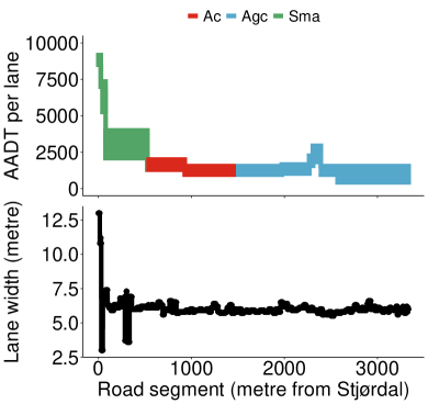
(a) AADT/Pavement type, and lane width

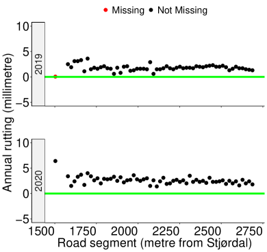
(b) Rutting

Figure 1: AADT together with pavement type, and lane width (a), and rutting (for years 2019-2020, mm/year — missing in red) (b).

2.4 Exploratory analysis of rutting

On average, over all stretches and years, rutting is $1.62$ mm/year; see Figure  2 (a). The density plots,  2 graph (b), show rutting for all segments for each year. Some years having higher rutting levels and are more widely distributed than others. The lines in graphs (c) and (d) give the correlation of rutting values with respect to distance (mean across all years, and two randomly selected years; 2011 and 2012, respectively) (Bachmaier and Backes 2011). It is computed from the observed rutting and shows how the rutting values are correlated with respect to distance between the corresponding segments. The distance (metre) is shown on the x-axis, and the calculated correlation between rutting values is on the y-axis. The graph shows some spatial dependencies of pavement rutting along the road. These exist for short distances of up to ($\sim$) $300$ metres (3 kilometres).

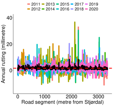
(a) Observed rutting

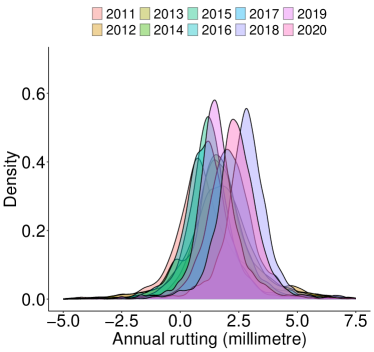
(b) Density

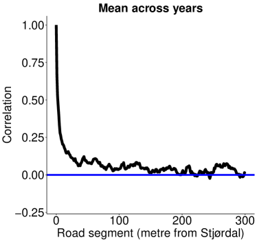
(c) Autocorrelation across years

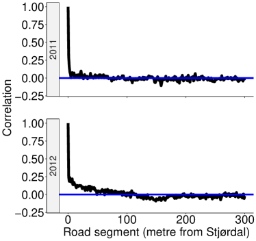
(d) Autocorrelation for years 2011-2012

Figure 2: Graph (a): Observed rutting for each year (2011-2020), observed mean rutting $1.62$ mm/year (     ), and the observed mean rutting across segments ( ). Graph (b): Rutting density plots, graph. Graphs (c) and (d) show how rutting values are correlated with distance. Spatial dependencies in rutting exist up to 3 kilometres.

3 Latent Gaussian models for Rutting

A Bayesian latent Gaussian model is a three-stage hierarchical model consisting of a likelihood, a latent Gaussian field, and hyperparameters. In this paper, the true rutting at location $s_{i}$ in year $t$ is denoted by $\eta_{t}(s_{i})$ and it is modelled as a latent Gaussian field that includes explanatory variables and spatial effects. We specify six (6) models with different explanatory variables included and with and without spatial and random effects.

3.1 Likelihood: observed rutting given true rutting

We denote the observed rutting for segment $i$ in year $t$ as $r_{i,t}$. The likelihood of the rutting, $r_{i,t}$, at road segment $i=1,...,n$ in year $t=1,...,T$ is expressed as

$$r_{i,t}\ |\ \eta_{t}(s_{i})\sim\mathrm{N}\left(\eta_{t}(s_{i}),\sigma^{2}_{\varepsilon}\right).$$ (3)

Here, $\sigma^{2}_{\varepsilon}$ is the uncertainty of the Gaussian observations. The unstructured error terms $\varepsilon_{i,t}\stackrel{{\scriptstyle i.i.d}}{{\sim}}\mathrm{Normal}(0,\sigma^{2}_{\varepsilon})$ are independent and identically distributed (i.i.d).

3.2 Latent field: model for true rutting

We model the observed rutting as Gaussian with expected value $\eta_{t}(s_{i})$ and variance $\sigma^{2}_{\varepsilon}$. Further, $r_{i,t}$ is conditionally independent, given the latent field $\eta_{t}(s_{i})$. We only consider models that have an interaction with AADT, and include a random yearly effect. It is known that more traffic gives more rutting, so we include traffic (AADT) in the model as an interaction with each of the explanatory variables. This means that for pavement type, we assume that the rutting is linear for all pavement types (double traffic means double rutting), but that the different pavement types can have different rates of deterioration. From the explanatory analysis (Figure 2), we found that the rutting seems to be on different levels for different years, and this might be explained by different weather conditions. To account for this, we include a random yearly effect in the model.

3.2.1 Non-spatial rutting model: based on explanatory variables and year effect

The model without spatial effects (non-spatial) has the linear predictor

$$\centering\begin{split}\eta_{t}(s)&=\beta_{\mathrm{Ac}}z_{\mathrm{Ac}(s,t)}+\beta_{\mathrm{Agc}}z_{\mathrm{Agc}(s,t)}+\beta_{\mathrm{Sma}}z_{\mathrm{Sma}(s,t)}+\beta_{\mathrm{d-1}}z_{\mathrm{d-1}(s,t)}+\beta_{\mathrm{w}}z_{\mathrm{w}(s,t)}+\gamma_{t}.\end{split}\@add@centering$$ (4)

The model assumes that the level of expected rutting (mm/year) is influenced by an interaction effect of the annual average daily traffic (AADT) and some explanatory variables, including the level of rut depth from the previous year ($z_{\mathrm{d-1}}$), the lane width ($z_{\mathrm{w}}$) and pavement type. Technically, $z_{Ac}(s,t)$ is

$$\begin{cases}\text{AADT (in ten thousands) if pavement at ($s,t$) is Ac,}\\ 0\ \text{if not Ac;}\\ \end{cases}$$

similarly, for pavement types Agc and Sma, representing asphalt gravel concrete and stone mastic asphalt, respectively. The effect of lane width, say, on rutting is dependent on the traffic intensity. The random yearly effect is assumed to be distributed as $\displaystyle\boldsymbol{\gamma}=(\gamma_{1},\gamma_{2},...,\gamma_{T}){\sim}\mathrm{Normal}(\boldsymbol{0}_{T},\ \tau_{\gamma}^{-1})$.

3.2.2 Models including spatial effects

There are several variables not included in our model (Equation (4)) that are known to influence rutting. Examples are variables related to weather, bearing capacity and proportion of heavy traffic load. Most of these variables are spatially dependent, and segments close in space are likely to be more similar than segments further a part. This can be accounted for and utilised by including spatial random effects. The spatial random effect is a Gaussian process (GP) along the road and can be interpreted as the part of the model not explained by the explanatory variables; lane width, rut depth from the previous year and pavement type that is spatially dependent. Further, it is reasonable that some of the spatial random effect is consistent over years (e.g., bearing capacity, side slope height, surface and base curvature and proportion of heavy traffic) while others vary between years (e.g., heavy rain events or more heavy traffic due to construction work). Therefore, we include both an annually varying spatial process $\xi_{t}(\boldsymbol{s})$ for year $t=1,...,T$, and a common spatial process $\omega(\boldsymbol{s})$, which we refer to as the spatial rutting component. The spatial rutting component is the spatial contribution to the total rutting that is not explained by the other variables e.g., variables in the non-spatial model in Equation (4). This contribution can either be positive or negative. The linear predictor for the model including spatial effects is described as

$$\eta_{t}(s) =\beta_{\mathrm{Ac}}z_{\mathrm{Ac}(s,t)}+\beta_{\mathrm{Agc}}z_{\mathrm{Agc}(s,t)}+\beta_{\mathrm{Sma}}z_{\mathrm{Sma}(s,t)}+\beta_{\mathrm{d-1}}z_{\mathrm{d-1}(s,t)}+\beta_{\mathrm{w}}z_{\mathrm{w}(s,t)}+$$ (5)

$$\gamma_{t}+\xi_{t}(s)+\omega(s),$$

where the remaining model parameters are defined as that in Equation 4.

The common spatial process $\omega(\boldsymbol{s})$ in Equations (5) is the time constant variable that can give rutting not explained by known variables (or unexplained rutting). It is a Gaussian random process $\left\{\omega(\boldsymbol{s}):\boldsymbol{s}\in\mathcal{D}\subseteq\mathbb{R}^{d}\right\}$ such that for any $n\geq 1$ and for each set of spatial locations $\left(s_{1},...,s_{n}\right)$ satisfies

$$\omega(\boldsymbol{s})=\left\{{\omega}(s_{1}),...,{\omega}(s_{n})\right\}=\left({\omega}_{1},...,{\omega}_{n}\right)\sim\mathrm{Normal}\left(\boldsymbol{\mu}^{\omega},\Sigma^{\omega}\right),$$ (6)

where $\boldsymbol{\mu}^{\omega}=\left\{\mu^{\omega}(s_{1}),...,\mu^{\omega}(s_{n})\right\}$ is the mean vector and $\Sigma^{\omega}_{ij}=\mathrm{Cov}\left\{\omega(s_{i}),\omega(s_{j})\right\}=C^{\omega}\left\{\omega(s_{i}),\omega(s_{j})\right\}$ are the elements of the covariance matrix defined by the Matérn stationary isotropic covariance function. Simply, this covariance is expressed as $C^{\omega}\left(d;\sigma^{2}_{\omega},\rho_{\omega}\right)$, where $d=||s_{i}-s_{j}||$ is the distance between two road segments; $\sigma^{2}_{\omega(s)}$ is the marginal variance of the spatial rutting component and $\rho_{\omega}$ is the spatial range for the spatial rutting component. These are the parameters to be estimated.

Similarly for the annually varying spatial field $\xi_{t}(\boldsymbol{s})$, the parameters to be estimated are $\sigma^{2}_{\xi_{t}}$ and $\rho_{t}$. Detail description of the Matérn covariance structure is found in (e.g., Blangiardo and Cameletti 2015, Krainski et al. 2018) and the Supplementary Material LABEL:supplementary:modelformula_SUPPLEMENTARY.

3.2.3 Other models for comparison

We consider simpler non-spatial and spatial models for comparison. These models include some of the known explanatory variables and are presented in Table 2. The most complex spatial model (in Equation 5) we refer to as Model 1, and it’s non-spatial version, Equation (4), as Model 4. These models include all three explanatory variables.

Table 2: Statistical models fitted

NAME		MODEL DESCRIPTION
		SPATIAL
Model 1		$\eta_{t}(s)=\beta_{\mathrm{Ac}}z_{\mathrm{Ac}(s,t)}+\beta_{\mathrm{Agc}}z_{\mathrm{Agc}(s,t)}+\beta_{\mathrm{Sma}}z_{\mathrm{Sma}(s,t)}+\beta_{\mathrm{d-1}}z_{\mathrm{d-1}(s,t)}+\beta_{\mathrm{w}}z_{\mathrm{w}(s,t)}+\gamma_{t}+\xi_{t}(s)+\omega(s)$
Model 2		$\eta_{t}(s)=\beta_{\mathrm{Ac}}z_{\mathrm{Ac}(s,t)}+\beta_{\mathrm{Agc}}z_{\mathrm{Agc}(s,t)}+\beta_{\mathrm{Sma}}z_{\mathrm{Sma}(s,t)}+\beta_{\mathrm{d-1}}z_{\mathrm{d-1}(s,t)}+\gamma_{t}+\xi_{t}(s)+\omega(s)$
Model 3		$\eta_{t}(s)=\beta_{\mathrm{Ac}}z_{\mathrm{Ac}(s,t)}+\beta_{\mathrm{Agc}}z_{\mathrm{Agc}(s,t)}+\beta_{\mathrm{Sma}}z_{\mathrm{Sma}(s,t)}+\gamma_{t}+\xi_{t}(s)+\omega(s)$
		NON-SPATIAL
Model 4		$\eta_{t}(s)=\beta_{\mathrm{Ac}}z_{\mathrm{Ac}(s,t)}+\beta_{\mathrm{Agc}}z_{\mathrm{Agc}(s,t)}+\beta_{\mathrm{Sma}}z_{\mathrm{Sma}(s,t)}+\beta_{\mathrm{d-1}}z_{\mathrm{d-1}(s,t)}+\beta_{\mathrm{w}}z_{\mathrm{w}(s,t)}+\gamma_{t}$
Model 5		$\eta_{t}(s)=\beta_{\mathrm{Ac}}z_{\mathrm{Ac}(s,t)}+\beta_{\mathrm{Agc}}z_{\mathrm{Agc}(s,t)}+\beta_{\mathrm{Sma}}z_{\mathrm{Sma}(s,t)}+\beta_{\mathrm{d-1}}z_{\mathrm{d-1}(s,t)}+\gamma_{t}$
Model 6		$\eta_{t}(s)=\beta_{\mathrm{Ac}}z_{\mathrm{Ac}(s,t)}+\beta_{\mathrm{Agc}}z_{\mathrm{Agc}(s,t)}+\beta_{\mathrm{Sma}}z_{\mathrm{Sma}(s,t)}+\gamma_{t}$

3.3 Prior models

The priors on the explanatory variables $\boldsymbol{\beta}=(\beta_{\mathrm{Ac}},\beta_{\mathrm{Agc}},\beta_{\mathrm{Sma}},\beta_{\mathrm{d-1}},\beta_{\mathrm{w}})$; and the hyperparameters for the random yearly effect $\gamma$ are assumed as follows

$$\begin{cases}\boldsymbol{\beta}\stackrel{{\scriptstyle i.i.d}}{{\sim}}\mathrm{Normal}(0,0.001^{-1})\\ \tau_{\gamma}\sim\mathrm{Gamma(0,\ 5.10^{-5})}\\ \sigma_{\varepsilon}\sim\mathrm{Gamma}(0,\ 5.10^{-5}).\end{cases}$$

Vague priors are used, and we let the data inform about the parameters to be estimated. The random yearly effect is evident in density plots in Figure 2 (c), which shows the varying yearly effect of rutting. For easier interpretations, the priors for the spatial components $\xi_{t}(s)$ and $\omega(s)$ are set through the spatial range $\rho$ and marginal standard deviation $\sigma_{\omega}(s)$ of the GRFs with Matérn covariance function in Equation (LABEL:eqn:randge_sigma_2). These are acquired jointly following the penalized complexity (PC) framework (Simpson et al. 2017, Fuglstad et al. 2019). The prior for the range is set through the probability $\mathrm{Pr}(\rho<250)=0.15$, indicating that there is a 15 percent probability that the spatial range is less than 250 metres. For the marginal standard deviation, the prior is set through the probability Pr$(\sigma_{\omega(s)}>2.5)=0.05$, indicating that there is a 5 percent probability that the marginal standard deviation for the rutting is over 2.5 millimetres. These priors are the same for all the spatial fields.

3.4 Inference and implementation

In Bayesian statistics, inference is done by computing posterior distributions for the parameters of interest based on prior models (Section 3.3), the likelihood model in Equation (3) and the data. Our goal is to estimate the marginal posteriors of the spatial rutting component, the regression coefficients, the hyperparameters and the expected rutting (marginal likelihood), given the known explanatory variables. We use INLA (integrated nested Laplace approximation) (Rue et al. 2009a, 2017, Martino and Riebler 2019), which is implemented in the R package R-INLA to approximate these marginal distributions.

3.5 Model evaluation

Three model fit measures are available; the deviance Information Criterion (DIC) (Spiegelhalter et al. 2002), the Watanabe-Akaike Information criterion (WAIC) (Watanabe and Opper 2010, Gelman et al. 2014) and the log-likelihood (Hubin and Storvik 2016) can be obtained for each of them in order to select the best one. The DIC and WAIC are based on hierarchical modeling generalizations of the Akaike Information Criterion (Akaike 1974), and are widely used in Bayesian statistics to perform model comparison. The values are determined by the model fit and its complexity, and by a penalty applied for overfitting. Models should balance complexity and goodness-of-fit, and models with the lowest DIC and WAIC should be chosen.

4 Results and discussion

We fit the models in Section 3.2.3 to the data in Section 2.3. For interpretability, the explanatory variables are standardized by subtracting the mean and dividing by the standard deviation. The results from the spatial Model 1 and the non-spatial version Model 4 are used to demonstrate the models’ performance. Based on Model evaluation criteria (Table 5), and for easy comparison of the models, the spatial and non-spatial models with more explanatory variables are selected. The results for the remaining models are given in Appendix A.

4.1 Estimated spatial rutting component and yearly effect

We analyze estimates from Model 1, identifying areas with high rutting rates not explained by AADT, pavement type, and lane width. The spatial rutting component ()$\hat{\omega}(s)$) plotted in Figure 3(a), varies significantly along the road. Some locations exhibit up to $3.15$ mm/year extra rutting beyond what is accounted for by known factors, while others show rutting exceeding $2$ mm/year. Conversely, the minimum unexplained rutting is $-2.45$ mm/year, indicating better performance than expected.

Figure 3(b) presents estimates of the random yearly $\hat{\gamma}_{t}$. Rutting varies notably between years for spatial and non-spatial models, with minimum estimates in 2016 and maximum in 2018. A systematic shift between spatial and non-spatial models is evident, particularly in pavement type coefficients (see Table 3 in Section 4.2).

Including spatial components in the model enhances rutting variability explanation and identifies areas with unexplained high rutting rates. This is confirmed in Figure 3 (b), where the rutting explained by the random yearly effect from the spatial model is at least $0.5$ mm/year less compared with the non-spatial model. Further discussion on estimated regression coefficients is in Section 4.2.

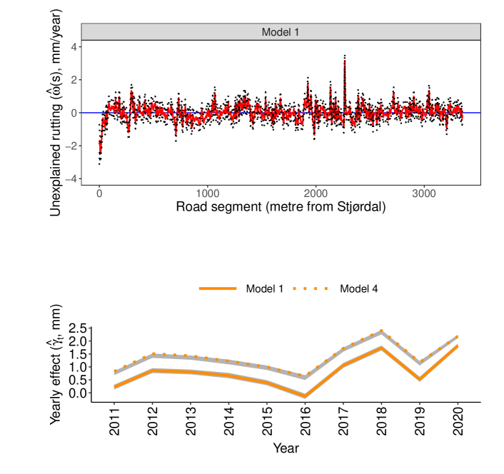
Figure 3: Upper panel: Spatial rutting component (unexplained rutting, $\hat{{\omega}}(s)$), with 95% credible interval. Lower panel: Rutting from the random yearly effect ($\hat{{\gamma}_{t}}$) from Model 1 ( ) and Model 4 (       ), with 95 % credible interval.

4.2 Estimated model parameters

The estimated parameters and 95% credible intervals (CI) for spatial (Model 1) and non-spatial (Model 4) are shown in Table 3. Spatial models exhibit notably higher estimates for pavement type coefficients compared with non-spatial models (see also Table A.2 in Appendix A). Moreover, models lacking the spatial rutting component display larger variance in the ‘noise’ term ($\hat{\sigma}{\varepsilon}$), suggesting that the spatial rutting component captures unobservable spatially varying factors such as weather and traffic.

Additionally, the spatial model better explains expected rutting, as indicated by smaller ‘noise’ terms ($\hat{\sigma}{\varepsilon}$) and uncertainty in random year effects ($\hat{\sigma}_{\gamma}$) compared with non-spatial models (refer to Table 3 and Table 4 in Appendix A). Further results are provided in Supplementary Materials LABEL:supplementary:addional_results.

Table 3: Estimated model parameters with $95\%$ credible intervals

	Spatial Model		Non-spatial Model
	Model 1		Model 4
	Mean/Median	95% CI	Mean/Median	95% CI
$\hat{\beta}_{\mathrm{Ac}}$	7.09	[6.56, 7.61]	3.27	[2.84, 3.71]
$\hat{\beta}_{\mathrm{Agc}}$	7.31	[6.08, 7.73]	3.24	[2.78, 3.70]
$\hat{\beta}_{\mathrm{Sma}}$	3.53	[3.26, 3.80]	2.03	[1.84, 2.22]
$\hat{\beta}_{\mathrm{d-1}}$	0.76	[0.68, 0.84]	1.07	[0.98, 1.17]
$\hat{\beta}_{\mathrm{w}}$	0.07	[0.01, 0.13]	0.05	[-0.02, 0.11]
$\hat{\sigma}_{\omega(s)}$	0.48	[0.45, 0.52]	-	-
$\hat{\sigma}_{\gamma}$	0.92	[0.63, 1.42]	1.37	[0.94, 2.10]
$\hat{\sigma}_{\varepsilon}$	1.38	[1.38, 1.39]	1.54	[1.53, 1.56]

4.2.1 Effects of the explanatory variables

Pavement types, particularly those with weaker binder concentrations like asphalt gravel concrete ($\hat{\beta}_{\mathrm{Agc}}$) and asphalt concrete ($\hat{\beta}_{\mathrm{Ac}}$), experience more rutting (Table 3). Qian et al. (2019) and Mascarenhas et al. (2020) shed light on how temperature and heavy traffic ($>$ 3.5 tonnes) impact rutting resistance on pavement types such as Agc and Ac. Notably, asphalt gravel concrete is predominantly situated approximately 30 kilometers from the Swedish border, where a sub-arctic climate, underdeveloped networks, and heavy traffic converge to adversely affect pavement performance Peel et al. (2007), Ketzler et al. (2021), Jenelius (2010), Hovi et al. (2018), Pinchasik et al. (2020). There is also greater uncertainty in asphalt concrete ($\hat{\beta}_{\mathrm{Ac}}$) and asphalt gravel concrete ($\hat{\beta}_{\mathrm{Agc}}$) compared with stone mastic asphalt ($\hat{\beta}_{\mathrm{Sma}}$), although considering spatial dependencies helps to explain more of the variability. Non-spatial models appear to explain variability between years rather than by pavement type, suggesting a nuanced relationship between these factors in understanding rutting susceptibility.

Rut depth from the previous year ($\hat{\beta}_{\mathrm{d-1}}$) becomes more crucial without accounting for spatial variability (Model 4, Table 3). The estimated effect of lane width ($\hat{\beta}_{\mathrm{w}}$) is minimal and positive, suggesting negligible impact on expected rutting.

These findings indicate that changes in coefficients are significant when spatial dependencies of unmodeled factors (e.g., weather) are considered. Furthermore, the spatial model captures more uncertainty (smaller $\hat{\sigma}_{\varepsilon}$).

4.3 Estimated rutting from the explanatory variables, random yearly effect and spatial rutting component

We employ Model 1 to identify maintenance ‘hot spots’ where intervention is most critical. This model combines rutting inference from explanatory variable coefficients ${\hat{\beta}_{(\cdot)}}$, the mean of the yearly random effects ($\hat{\gamma}$), and the spatial rutting component ${\hat{\omega}(s)}$. Since the yearly random effects ($\gamma_{t}$) vary annually, we use an estimate of their mean, denoted as $\hat{\gamma}$. The yearly variation in ($\hat{\sigma}_{\xi_{t}}$) is small annually (Supplementary Materials LABEL:supplementary:addional_results), so it is not considered in our analysis. We account for both explained and unexplained rutting.

Initially, rutting estimation relies on explanatory variables and the yearly random effect ($\hat{\eta}^{*}=\hat{\beta}_{{(1)}}z_{(1)(\mathrm{s,t})}+\hat{\gamma}$), with each asphalt type highlighted as Sma ( ), Ac ( ), and Agc ( ) (see Figure 4, graph (a)). Incorporating spatial rutting components yields a more comprehensive estimation ${\hat{\eta}=\hat{\beta}_{(1)}z_{(1)(\mathrm{s,t})}+\hat{\gamma}+\hat{\omega}(s)}$. A comparison of these estimates highlights the influence of spatial components.

The results indicate less variability in rutting estimates without spatial components (ranging from $0.97$ to $3.64$ mm/year) compared to estimates including spatial factors (ranging from $-0.44$ to $4.67$ mm/year). This suggests that explanatory variables and the random yearly effect alone do not fully capture or represent the true rutting variability. Including spatial and yearly effects provides a more comprehensive understanding of rutting variability. Tables 3 and 4 in Appendix A demonstrate this, with the remaining uncertainty ($\hat{\sigma}_{\varepsilon}$) lower in the spatial model ($1.38$ mm/year) compared to the non-spatial model ($1.54$ mm/year).

The findings indicate that high rutting estimates could arise from explanatory variables, while moderate estimates, coupled with large spatial rutting components, suggest the influence of other factors.

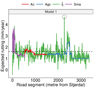
(a) $\hat{\eta}^{*}$, $\hat{\eta}$ and mean rutting $1.62$ mm/year (       ).

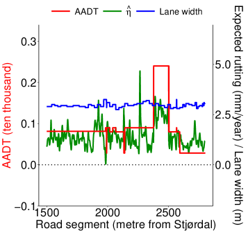
(b) $\hat{\eta}$, AADT and lane width

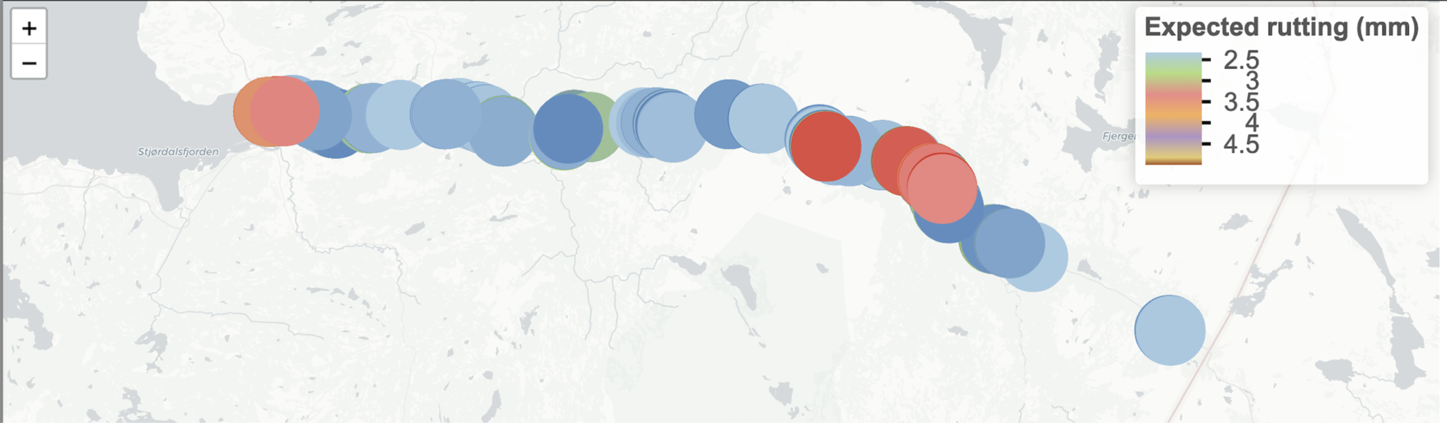
(c) $\hat{\eta}>2$ mm

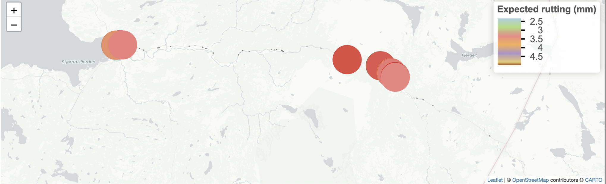
(d) $\hat{\eta}>3$ mm.

Figure 4: Graph (a): Expected rutting from: i) $\hat{\eta}$ and ii) from $\hat{\eta}{{}^{*}}$, with each asphalt type highlighted. The effects are inferred for the year 2020. Graph (b): Expected rutting plotted against AADT and lane width for a short stretch. Graphs (c) and (d) give the locations where rutting exceeds $2$ mm/year and $3$ mm/year, respectively.

4.3.1 Comparing expected rutting with observed data

The observed mean rutting (Figure 2 (a) in Section 2.4) stands at $1.62$ mm/year. In Figure 4, graph (a), 361 road segments have an expected rutting exceeding this mean, with 49 segments showing estimated rutting exceeding $3$ mm/year (graphs (c) and (d), respectively). These 49 locations signify potential hot spots for accelerated rutting, necessitating urgent maintenance, as their expected lifetime could be as short as 8 years, depending on traffic. Additionally, the observed mean rutting across segments ranges from -0.14 to 8.33 mm/year (Figure 2, graph (a)), while the maximum expected rutting from the model is 4.67 mm/year (Figure 4, graph (a)), approximately half the maximum observed mean rutting.

In Figure 4, graph (b), we plot the expected rutting $\hat{\eta}$, lane width, and AADT (per ten thousand) for a short road section spanning segments $1500-2700$ (or $30-54$ km from Stjørdal), characterized by weaker pavement type Agc. This section exhibits spikes of accelerated rutting, particularly evident with increasing traffic. Possible factors contributing to this variability include changes in asphalt type, traffic composition, suboptimal road design, or inadequate pavement maintenance.

4.4 Investigating an area with high rutting rates

The significant spike in Figure (4) (a), indicating high rutting rates, prompts further investigation. We examine road segments spanning 2100 to 2700 meters surrounding this spike, located in the municipality of Meråker, just 20 kilometers west of the Swedish border at Storlien. This stretch, depicted in Figure 4 (a), exhibits notably high rutting, peaking at $4.67$ mm, with an estimated lifespan of only $5$ years (in a low-traffic area requiring maintenance at 25 mm rut depth). Possible contributors to this accelerated rutting include clogged drainage, flooding, absence of side ditches (see Figure 5), heavy traffic, or road designs featuring railguards installed close to the lane edge, which encourages traffic to remain within the same wheel tracks (refer to Figure A.4 in Appendix A.4). Meråker’s industrial and agricultural activities result in increased traffic from heavy vehicles, including farm equipment such as tractors (industrial, wheel drive, row crop).

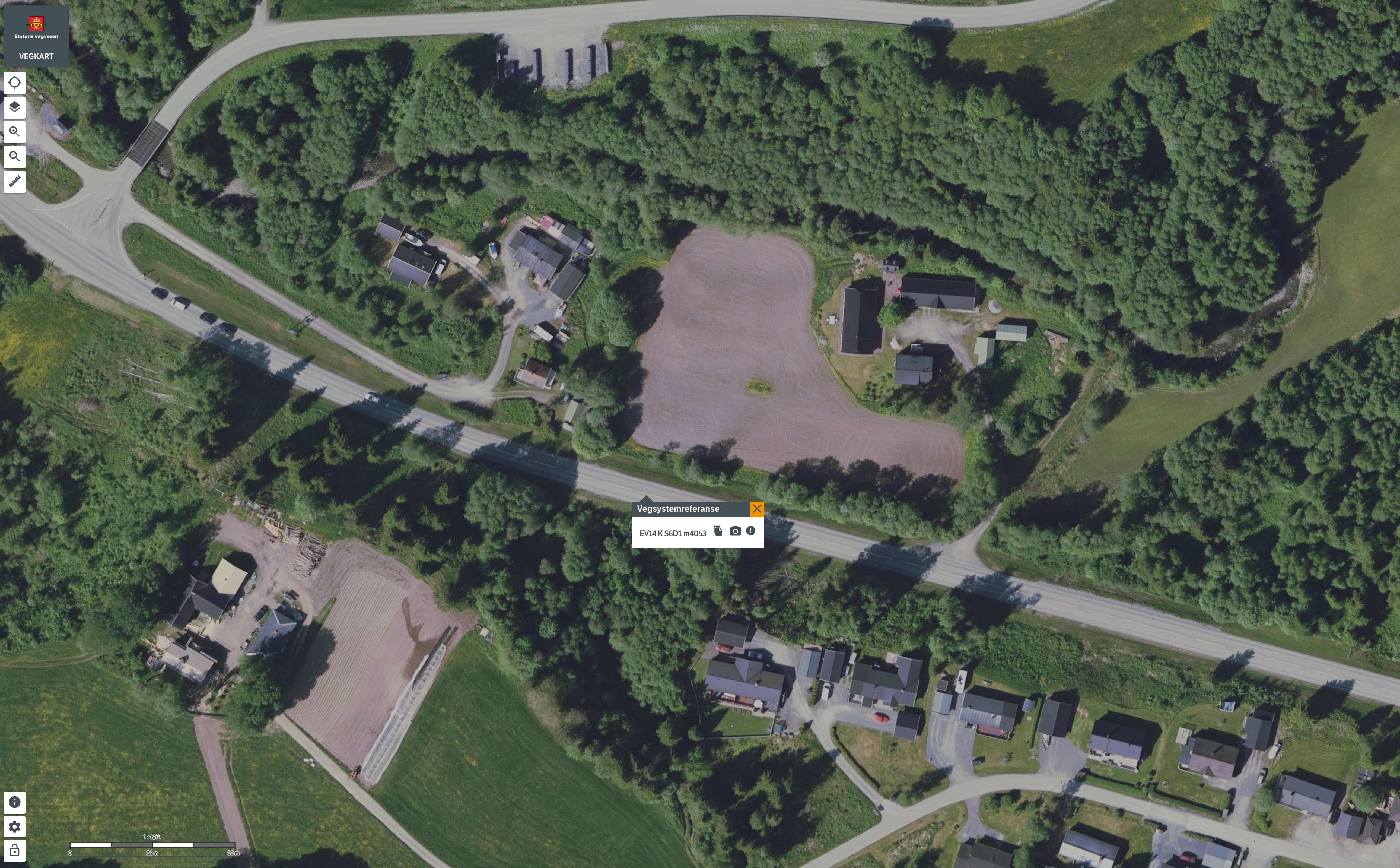
(a) Short section between EV14 S6D1 m3841-m4285 F1 with high rutting.

(b) Location EV14 S6D1 m4068 F1 in year 2020

(c) Location EV14 S6D1 m4059 F1 in year 2021

(d) Location EV14 S6D1 m4065 F1 in year 2022

Figure 5: Graph (a): Location with high rutting rates (road segments $2100-2700$ towards Sweden). Graphs (b), (c) and (d) show the location, in years 2020-2022 (see Statens vegvesen or url: https://vegkart.atlas.vegvesen.no/#kartlag:nib/@335074,7038866,15/vegsystemreferanse:335035.067:7038844.352

4.4.1 Exploring the spatial model with various values of the explanatory variables

To further investigate high rutting values in a road section, we analyze the impact of explanatory variables, yearly variation, and spatial rutting component ($\hat{\eta}$). We explore spatial Model 1 using different values for variables to estimate rutting. First, we use actual measurements like asphalt type, lane width, and rut depth ($\hat{\eta}_{\mathrm{True}}$). Second, we consider alternative asphalt types - asphalt concrete (Ac) or stone mastic asphalt (Sma) ($\hat{\eta}_{\mathrm{Ac}}$ or $\hat{\eta}_{\mathrm{Sma}}$). Third, we examine extreme values such as the strongest pavement (Sma), minimal rut depth (0.01 mm), or wider lanes (6 meters) ($\hat{\eta}_{\mathrm{Best}}$). Conversely, accelerated rutting scenarios involve deeper rut depth (25 mm), narrower lanes (2.75 meters), and asphalt gravel concrete (Agc) ($\hat{\eta}_{\mathrm{Worse}}$) from the E14 dataset. These scenarios are depicted in Figure 6 (a).

With worse values ( ), rutting is projected to be at least 1.5 mm/year ($1.76-8.20$), indicating accelerated deterioration and the need for maintenance within 3 to 14 years. Locations with unexpectedly high rutting, exceeding 4 mm/year, are observed, possibly due to increased AADT compared to other areas (Figure 4, graph b).

Using the best covariate values ( ), rutting is projected to be at most 4.30 mm/year, with maintenance required approximately 6 years after construction or maintenance. Additionally, using the stronger asphalt binder Sma yields similar rutting estimates but generally lower than those using the best values, indicating asphalt type as a primary factor. Asphalt gravel concrete (Agc,  ) and asphalt concrete (Ac,  ) show similar rutting estimates due to similar binder concentrations.

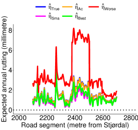
(a) Expected rutting at road segments $2100-2500$ (metres) towards Sweden.

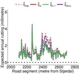
(b) Expected rutting from adding each explanatory variable added sequentially.

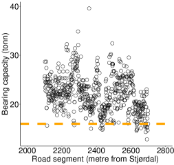
(c) Bearing capacity (tonn).

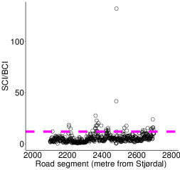
(d) SCI/BCI.

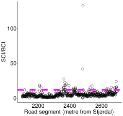
(e) SCI/BCI for the whole E14.

Figure 6: Graph (a) displays expected rutting using spatial rutting component $\hat{\omega}(s)$ for road segments $2100-2700$, along with the ’best’ or ’worst’ explanatory values. $\hat{\eta}_{\mathrm{Agc}}$ represents pavement type Agc, random yearly effect $\hat{\gamma}$, and $\hat{\omega}(s)$. Graph (b) illustrates expected rutting inferred from $\hat{\omega}(s)$, $\hat{\gamma}$, and sequentially added explanatory variables. Graph (c) shows 2021 bearing capacity in tons; values $\geq$ 16 indicate good parameters. Graphs (d) and (e) depict SCI to BCI ratios for a short stretch or the entire E14; values $<$ 12 indicate good curvature index.

We examine the impact of pavement type on rutting (Figure 6, graph (b)). Changing from asphalt type Agc (asphalt gravel concrete) to the stronger Sma (stone mastic asphalt) while keeping all other variables constant, we sequentially add additional explanatory variables to the model, starting with pavement type. Initially, pavement type (Agc or Sma) is included with the random yearly effect $\hat{\gamma}$ and the spatial rutting component $\hat{\omega}(s)$ as follows: $\hat{\tilde{\eta}}_{\mathrm{Agc}}=\hat{\beta}_{\mathrm{Agc}}z_{\mathrm{Agc(s,t)}}+\hat{\gamma}+\hat{\omega}(s)$ or $\hat{\tilde{\eta}}_{\mathrm{Sma}}=\hat{\beta}_{\mathrm{Sma}}z_{\mathrm{Agc(s,t)}}+\hat{\gamma}+\hat{\omega}(s)$. Subsequently, the previous year’s rut depth is incorporated, represented as $\hat{\tilde{\eta}}_{\mathrm{d-1}}=\hat{\beta}_{\mathrm{Agc}}z_{\mathrm{Agc(s,t)}}+\hat{\beta}_{\mathrm{d-1}}z_{\mathrm{d-1(s,t)}}+\hat{\gamma}+\hat{\omega}(s)$ or $\hat{\tilde{\eta}}_{\mathrm{d-1}}=\hat{\beta}_{\mathrm{Sma}}z_{\mathrm{Sma(s,t)}}+\hat{\beta}_{\mathrm{d-1}}z_{\mathrm{d-1(s,t)}}+\hat{\gamma}+\hat{\omega}(s)$. Similarly, the model with added lane width ${\hat{\beta}_{w}z_{\mathrm{w(s,t)}}}$ is denoted as $\hat{\tilde{\eta}}_{\mathrm{w}}$. Results from using stone mastic asphalt (Sma) are depicted by solid lines, and asphalt gravel concrete (Agc) results are shown with dotted lines.

The findings affirm that pavement type significantly influences rutting. Implementing the stronger binder type Sma instead of the actual pavement type Agc would decrease expected rutting, reaching a maximum of $4.35$ mm/year (compared to 4.68 mm/year), approximately reducing rutting by 0.33 mm/year annually. Over a projected lifetime of 6 years, this equates to an additional year of serviceability.

4.4.2 Evaluating pavement subgrade support on expected rutting

We examine bearing capacity, surface curvature index (SCI), and base curvature index (BCI) for road segments 2100-2700 using 2021 data, indicative of construction quality and soil pressure sustainability over the past decade (Figure 6, graph (c)). Bearing capacity values exceeding 16 tons (       ) suggest a robust foundation design. The SCI to BCI ratio (Figure 6, graphs (d) and (e)) reveals deflection location within the pavement layers. High rutting may result from factors like side slope height (data unavailable), inadequate drainage, or sub-base layer deformation during thawing periods. Bearing capacity data, sampled and temperature-corrected during summer, may inflate measurements compared to thawing periods. Varying construction material quality along the road stretch (segments 1500-3355) warrants investigation into surface and subsoil layer deflections. An SCI/BCI ratio below 12 (       ) indicates robust construction. Inconsistent ratios suggest layer deformation, with data indicating uneven construction on E14, featuring deeper base layer deflections.

In conclusion, pavement type significantly influences rutting, recommending stronger binder types for extended lifespan.

5 How road authorities can make use of this model

The spatial-statistical model serves as a potent tool for road authorities, offering a data-driven approach to enhance maintenance strategies, identify critical areas for intervention, and optimize road infrastructure durability. This approach facilitates a more precise diagnosis of rutting, enabling authorities to make informed decisions for sustainable road infrastructure.

Our analyses reveal that rutting exceeding 2 mm/year is expected at several locations along E14. Given the expected lifetime of the pavement and recommended treatment levels, this level of rutting is concerning. Maintenance carried out at rut depths of 20-25 mm, depending on traffic, and pavement designs expected to last between 20-30 years indicate that some sections of the road may only survive for at most 12.5 years (10 years in high-traffic areas). It’s imperative to consider spatial rutting components; models fitted with variables known to influence rutting and random yearly effects alone underestimate rutting variability, thus inflating pavement lifetime estimates. Including the spatial rutting component reduces estimated pavement lifetimes to at most 6 years, compared to 5 years without it. This information is crucial for road authorities’ long-term planning and resource allocation.

We’ve demonstrated the spatial-statistical model’s ability to identify areas with unexpectedly high rutting, pinpointing hot spots where rutting is accelerating and indicating urgent maintenance needs. By analyzing factors influencing rutting, random effects, and spatial components, authorities can prioritize resources for targeted interventions. Additionally, the model provides a comprehensive understanding of rutting, enhancing authorities’ ability to make informed decisions about maintenance priorities and pavement materials during construction or rehabilitation.

The model can investigate contributing factors to rutting beyond pavement type, such as drainage issues, heavy traffic, and road design flaws. Comparisons with non-spatial models emphasize the importance of spatial factors in explaining rutting variations, reinforcing the need for spatial models for accurate inference and predictions. The estimated model parameters and credible intervals provide a robust foundation for data-driven decision-making, enabling road authorities to make informed choices regarding maintenance priorities and infrastructure improvements.

6 Conclusion

This research offers valuable insights into the rutting phenomenon by elucidating both well-established factors and those that remain unexplained. It shows the importance of incorporating spatial information to accurately estimate rutting variability, showing that observations in close proximity exhibit higher similarity than those at a distance. To achieve a comprehensive understanding, it is imperative to consider both observable elements like traffic and temperature, as well as unobservable factors like weather, and integrate spatial rutting components.

Moreover, the study confirms the significant impact of asphalt type selection on rutting performance, with rut-resistant mixtures proving more effective in mitigating rutting. Lane width also influences pavement rutting, with narrower roads experiencing more concentrated traffic loads and, consequently, increased rutting. Conversely, wider roads distribute traffic loads over a larger area, reducing rut formation.

The analysis reveals that wider road sections tend to experience higher rut depths compared to narrower road stretches. This result can be attributed to the increased traffic volumes and higher wheel loads present on wider roads, which contribute to more pronounced rutting. To address this issue and minimize rutting problems over time, it is advisable to integrate a life-cycle cost-benefit perspective into road design and planning processes.

Further research is encouraged to explore additional factors influencing rutting, such as bearing capacity, ditch depth for water outflow, and lane width. This would enhance the credibility of research results and the applicability of models to other road networks. Additionally, evaluating the long-term performance of rut-resistant asphalt mixtures under various traffic and environmental conditions would be worthwhile.

Disclosure Statement

The authors report no declarations of interest.

Funding

This work was supported by the Norwegian University of Science and Technology in collaboration with Statens Vegvesen Project [grant number 9056608 – Smarter Maintenance (2019-2023)].

7 Appendices

Appendix A Inference from model parameters

Table 4 compares estimates from the proposed spatial and non-spatial models. The results show that the spatial models account for uncertainty in factors that vary in space, e.g., weather and other explanatory variables such as bearing capacity and roadside ditches not included in the model. Including more explanatory variables reduces the ‘noise‘ term ($\hat{\sigma}_{\varepsilon}$) and random yearly effect ($\hat{\sigma}_{\gamma}$).

Table 4: Estimated model parameters with $95\%$ credible intervals

SPATIAL MODELS Model 1 Model 2 Model 3 Mean/Median 95% CI Mean/Median 95% CI Mean/Median 95% CI $\hat{\beta}_{\mathrm{Ac}}$ 7.09 [6.56, 7.61] 7.08 [6.55, 7.61] 6.89 [6.34, 7.44] $\hat{\beta}_{\mathrm{Agc}}$ 7.31 [6.88, 7.73] 7.29 [6.86, 7.71] 7.07 [6.64, 7.50] $\hat{\beta}_{\mathrm{Sma}}$ 3.53 [3.26, 3.80] 3.55 [3.28 3.82] 3.31 [3.03, 3.59] $\hat{\beta}_{\mathrm{d-1}}$ 0.76 [0.68, 0.84] 0.76 [0.68, 0.84] - - $\hat{\beta}_{\mathrm{w}}$ 0.07 [0.01, 0.13] - - - $\hat{\sigma}_{\omega(s)}$ 0.48 [0.45, 0.52] 0.48 [0.45, 0.52] 0.52 [0.48, 0.57] $\hat{\sigma}_{\gamma}$ 0.92 [0.63, 1.42] 0.93 [0.63, 1.40] 0.93 [0.63, 1.42] $\hat{\sigma}_{\varepsilon}$ 1.38 [1.38, 1.39] 1.38 [1.38, 1.39] 1.39 [1.38, 1.40] NON-SPATIAL MODELS Model 4 Model 5 Model 6 Mean/Median 95% CI Mean/Median 95% CI Mean/Median 95% CI $\hat{\beta}_{\mathrm{Ac}}$ 3.27 [2.84, 3.71] 3.28 [2.85, 3.72] 2.72 [2.29, 3.16] $\hat{\beta}_{\mathrm{Agc}}$ 3.24 [2.78, 3.70] 3.23 [2.77, 3.70] 2.71 [2.25, 3.17] $\hat{\beta}_{\mathrm{Sma}}$ 2.03 [1.84, 2.22] 2.05 [1.86, 2.24] 1.55 [1.36, 1.73] $\hat{\beta}_{\mathrm{d-1}}$ 1.07 [0.98, 1.17] 1.08 [0.98, 1.18] - - $\hat{\beta}_{\mathrm{w}}$ 0.05 [ -0.02, 0.11] - - - - $\hat{\sigma}_{\gamma}$ 1.37 [0.94, 2.10] 1.37 [0.94, 2.10] 1.41 [0.96, 2.17] $\hat{\sigma}_{\varepsilon}$ 1.54 [1.53, 1.56] 1.56 [1.54, 1.57] 1.56 [1.54, 1.57]

A.1 Model Comparison

Model comparison criteria (Table 5) select the models with more explanatory variables most often as the best model, with the highest goodness-of-fit (lowest DIC and WAIC). As shown in the results above (e.g., Table 4), the more complex spatial models (Model 1) and non-spatial models (Model 4 or 5) capture the random and spatial variability of pavement rutting and explains more of the unstructured error terms with the addition of explanatory variable lane width.

Table 5: Model comparison

Model	Estimates from spatial models			Model	Estimates from non-spatial models
	DIC	WAIC	(-) loglikelihood		DIC	WAIC	(-) loglikelihood
1	195067.76	195660.91	-101464.72	4	104290.61	100996.40	-52229.53
2	195154.12	195669.17	-101460.32	5	104290.62	100996.45	-52223.62
3	195242.58	195959.89	-101624.69	6	104763.10	101556.00	-52453.66

A.2 Marginal Posterior Distributions of Explanatory Variables

Figure A.2 gives the marginal posterior distributions of asphalt type, rut depth from the previous year and lane width. Narrow bands of the distributions indicate that the uncertainty is smaller. Graph (a) shows a clear shift in asphalt type’s contribution to rutting from the spatial and non-spatial models. This is because asphalt type is spatially varying. Stone mastic asphalt (Sma) gave lower rutting values because it has a stronger binder.

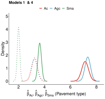
(a) Pavement type

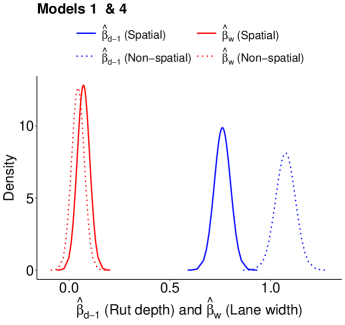
(b) Rut depth

Figure A.2: Marginal posterior distributions of pavement type (solid lines are the spatial models, and the dotted lines are the non-spatial models), rut depth from the previous year and lane width.

A.3 Marginal Posterior Distributions of Random Effects

Figure A.3 gives the marginal posterior distributions of the standard deviation of the Gaussian observations ($\hat{\sigma}_{\varepsilon}$), the standard deviation of the random yearly effect ($\hat{\sigma}_{\gamma}$), the range of the common spatial field $\hat{\rho}$, and the standard deviation of the common spatial field $\hat{\sigma}_{\omega(s)}$. The solid lines represent the spatial models and the dotted lines represent the non-spatial models. Narrower densities suggest smaller estimated uncertainty. We find that some of the uncertainty of the Gaussian observations $(\hat{\sigma}_{\varepsilon})$ and random yearly effect $(\hat{\sigma}_{\gamma})$ go into the spatial effect $\{\hat{\sigma}_{\omega(s)}\}$, and this can be interpreted as some of the unobserved variability (e.g., weather, temperature) being explained by the spatial rutting component; see Table 3 and Figure A.3 (a) and (b). This is confirmed by the smaller estimates of the ‘noise’ term $(\hat{\sigma}_{\varepsilon})$ compared with the non-spatial model (Table 4).

We examine the effects of the range of the common spatial field ($\hat{\rho}$), and the standard deviation of the common spatial field $\{\hat{\sigma}_{\omega(s)}\}$. As more explanatory variables are added to model (e.g., rut depth), the variability of the common spatial field $\{\hat{\sigma}_{\omega(s)}\}$ decreases; see Table 4 and Figure A.3, graph (d).

In Model 2, rut depth from the previous year is included, and this effect is large with the credible interval not covering zero. This indicates that deeper rut depths from the previous year would result in increased rutting; Figure A.2, graph (b). In addition, the spatial range for the common spatial field is, generally, larger for Model 2 compared with Model 3 (the simpler model), where rut depth is included (see Table LABEL:tab:range_for_each_year_appendix in Supplementary Material LABEL:supplementary:addional_results) for estimated $\hat{\rho}_{t}$ for each year). This is so, presumably, because of influenced factors such as varying weather patterns. But including lane width reduces the effect of rut depth on expected rutting.

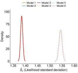
(a) Marginal posterior distributions of the standard deviation of the Gaussian observations $\hat{\sigma}_{\varepsilon}$.

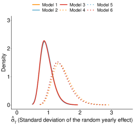
(b) Marginal posterior distributions of the standard deviation of the random yearly effect $\hat{\sigma}_{\gamma}$.

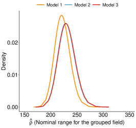
(c) Marginal posterior distributions of the nominal range of the common spatial field $\hat{\rho}$ .

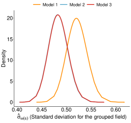
(d) Marginal posterior distributions of the standard deviation of the common spatial field $\hat{\sigma}_{\omega(s)}$.

Figure A.3: Estimates of marginal posterior distributions of the spatial models (solid lines) and non-spatial models (dotted lines).

A.4 Area with high rutting rates

Figure A.4 shows the location where rutting exceeds $7$ mm when the worse values of the explanatory variables are used to explore Model 1 (see Section 4.4)

(a) Short section between EV14 S6D1 m6802-m6882 F1 with high rutting.

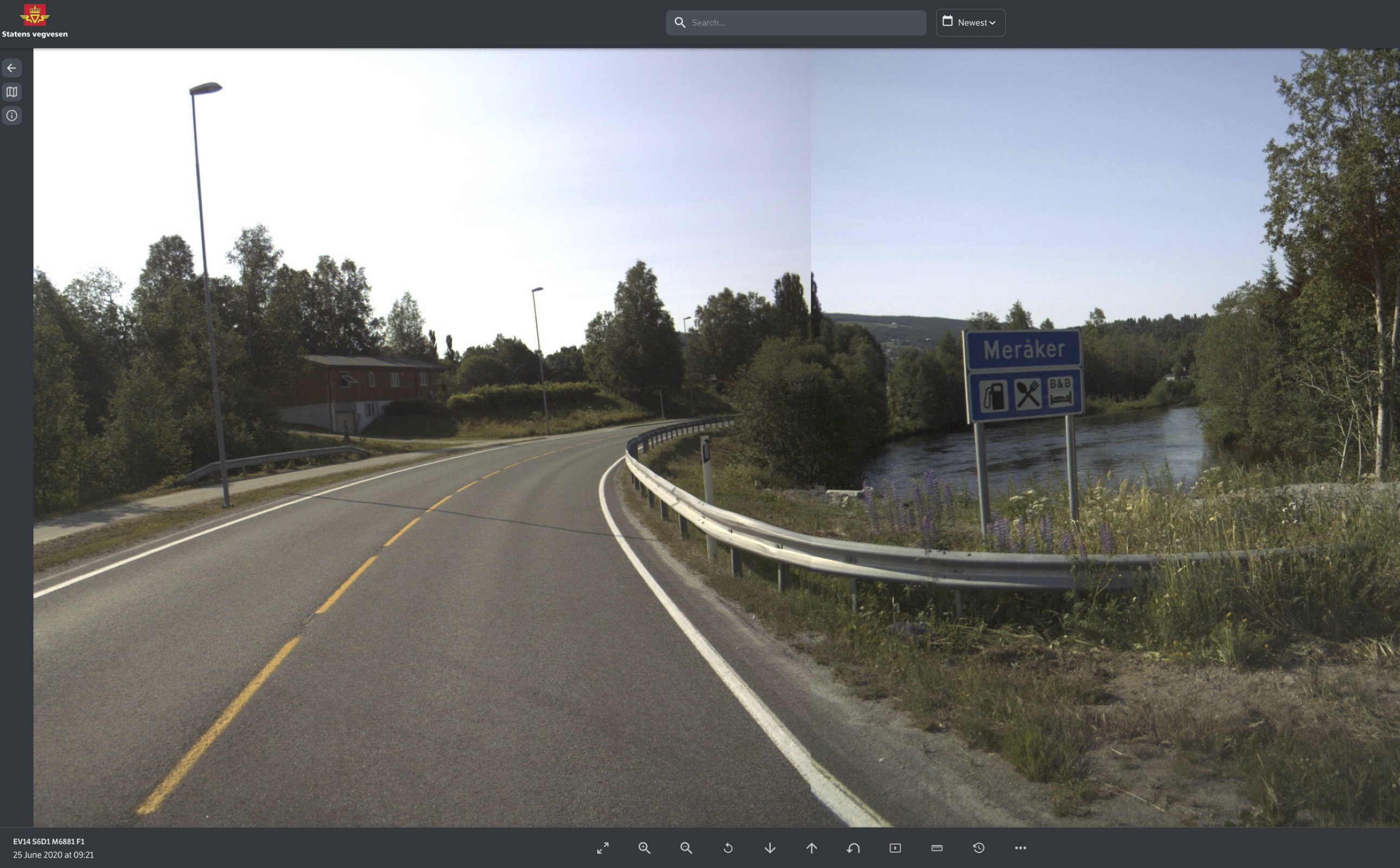
(b) Location EV14 S6D1 m6881 F1 in year 2020

(c) Location EV14 S6D1 m6808 F1 in year 2021

(d) Location EV14 S6D1 m6807 F1 in year 2022

Figure A.4: Graph (a): Location with high rutting rates (road segments $2100-2700$ towards Sweden). Graphs (b), (c) and (d) show the location, in years 2020-2022 (see Statens vegvesen or go to the next url: https://vegkart.atlas.vegvesen.no/#kartlag:nib/@337039,7037105,18/vegsystemreferanse:337039.29:7037149.25

References

- Akaike (1974) Akaike, H., 1974. A new look at the statistical model identification. IEEE transactions on automatic control, 19 (6), 716–723.
- Al-Khateeb and Basheer (2009) Al-Khateeb, G. and Basheer, I., 2009. A three-stage rutting model utilising rutting performance data from the Hamburg Wheel-Tracking Device (WTD). Road & Transport Research: A Journal of Australian and New Zealand Research and Practice, 18 (3), 12–25.
- Alhasan et al. (2018) Alhasan, A., et al., 2018. Incorporating spatial variability of pavement foundation layers stiffness in reliability-based mechanistic-empirical pavement performance prediction. Transportation Geotechnics, 17, 1–13.
- Archilla and Madanat (2000) Archilla, A.R. and Madanat, S., 2000. Development of a pavement rutting model from experimental data. Journal of transportation engineering, 126 (4), 291–299.
- Bachmaier and Backes (2011) Bachmaier, M. and Backes, M., 2011. Variogram or semivariogram? Variance or semivariance? Allan variance or introducing a new term? Mathematical Geosciences, 43 (6), 735–740.
- Banerjee et al. (2008) Banerjee, S., et al., 2008. Gaussian predictive process models for large spatial data sets. Journal of the Royal Statistical Society: Series B (Statistical Methodology), 70 (4), 825–848.
- Blangiardo and Cameletti (2015) Blangiardo, M. and Cameletti, M., 2015. Spatial and spatio-temporal Bayesian models with R-INLA. John Wiley & Sons.
- Chan et al. (2010) Chan, C.Y., et al., 2010. Investigating effects of asphalt pavement conditions on traffic accidents in Tennessee based on the pavement management system (PMS). Journal of advanced transportation, 44 (3), 150–161.
- Chen and Mastin (2016) Chen, D. and Mastin, N., 2016. Sigmoidal models for predicting pavement performance conditions. Journal of Performance of Constructed Facilities, 30 (4), 04015078.
- Cheng et al. (2023) Cheng, C., et al., 2023. Predicting Rutting Development of Pavement with Flexible Overlay Using Artificial Neural Network. Applied Sciences, 13 (12), 7064.
- Chou et al. (2008) Chou, E., et al., 2008. Pavement forecasting models. Ohio. Dept. of Transportation.
- Chu et al. (2005) Chu, W., Ghahramani, Z., and Williams, C.K., 2005. Gaussian processes for ordinal regression. Journal of machine learning research, 6 (7).
- Dey et al. (2000) Dey, D.K., Ghosh, S.K., and Mallick, B.K., 2000. Generalized linear models: A Bayesian perspective. CRC Press.
- d’Angelo et al. (2008) d’Angelo, J., et al., 2008. Warm-mix asphalt: European practice. United States. Federal Highway Administration. Office of International Programs.
- Ebrahimi et al. (2019) Ebrahimi, B., et al., 2019. Estimation of Norwegian asphalt surfacing lifetimes using survival analysis coupled with road spatial data. Journal of Transportation Engineering, Part B: Pavements, 145 (3), 04019017.
- Fuglstad et al. (2019) Fuglstad, G.A., et al., 2019. Constructing priors that penalize the complexity of Gaussian random fields. Journal of the American Statistical Association, 114 (525), 445–452.
- Gelman et al. (2014) Gelman, A., Hwang, J., and Vehtari, A., 2014. Understanding predictive information criteria for Bayesian models. Statistics and computing, 24 (6), 997–1016.
- Gu et al. (2017) Gu, F., et al., 2017. Characterization and prediction of permanent deformation properties of unbound granular materials for pavement ME design. Construction and Building Materials, 155, 584–592.
- Gudipudi et al. (2017) Gudipudi, P.P., Underwood, B.S., and Zalghout, A., 2017. Impact of climate change on pavement structural performance in the United States. Transportation Research Part D: Transport and Environment, 57, 172–184.
- Gupta et al. (2014) Gupta, A., Kumar, P., and Rastogi, R., 2014. Critical review of flexible pavement performance models. KSCE Journal of Civil Engineering, 18 (1), 142–148.
- Hao et al. (2009) Hao, W., Jian-Zhong, P., and ZHANG, J.p., 2009. Rutting law and its influence factors for asphalt pavement in long and steep longitudinal slope section. Journal of Chang’an University: Natural Science Edition, 29 (6), 28–31.
- Hovi et al. (2018) Hovi, I.B., et al., 2018. Measures for reduced CO2-emissions from freight transport in the Nordic countries. In: Proceedings from the Annual Transport Conference at Aalborg University. vol. 25.
- Hu et al. (2022) Hu, A., et al., 2022. A review on empirical methods of pavement performance modeling. Construction and Building Materials, 342, 127968.
- Hubin and Storvik (2016) Hubin, A. and Storvik, G., 2016. Estimating the marginal likelihood with Integrated nested Laplace approximation (INLA). arXiv preprint arXiv:1611.01450.
- Institutt (2010) Institutt, M., 2010. Ekstremvarsel. Meteorologisk Institutt, 12.
- Jacobson and Wågberg (2005) Jacobson, T. and Wågberg, L.G., 2005. Prediction models for pavement wear and associated costs. VTI., VTI särtryck 366A.
- Jenelius (2010) Jenelius, E., 2010. Large-scale road network vulnerability analysis. Thesis (PhD). KTH.
- Jourdain and Klein-Paste (2024) Jourdain, Natoya OAS, S.I.B.S.M.G.S.D. and Klein-Paste, A., 2024. A spatial-statistical model to analyse historical rutting data, [https://doi.org/10.48550/arXiv.2401.03633]. arXiv.
- Ketzler et al. (2021) Ketzler, G., Römer, W., and Beylich, A.A., 2021. The Climate of Norway. In: Landscapes and landforms of norway. Springer, 7–29.
- Korkiala-Tanttu and Dawson (2007) Korkiala-Tanttu, L. and Dawson, A., 2007. Relating full-scale pavement rutting to laboratory permanent deformation testing. International Journal of Pavement Engineering, 8 (1), 19–28.
- Krainski et al. (2018) Krainski, E., et al., 2018. Advanced spatial modeling with stochastic partial differential equations using R and INLA. Chapman and Hall/CRC.
- Lang (2012) Lang, J., 2012. Comparison of pavement management in the nordic countries: Paper prepared for 4th EPAM CONFERENCE.
- Lea and Harvey (2015) Lea, J.D. and Harvey, J.T., 2015. A spatial analysis of pavement variability. International Journal of Pavement Engineering, 16 (3), 256–267.
- Li et al. (2023) Li, L., et al., 2023. A Design Method on Durable Asphalt Pavement of Flexible Base on Anti-Rutting Performance and Its Application. Materials, 16 (22), 7122.
- Lindgren and Rue (2015) Lindgren, F. and Rue, H., 2015. Bayesian spatial modelling with R-INLA. Journal of statistical software, 63, 1–25.
- Lundy et al. (1992) Lundy, J.R., et al., 1992. Wheel track rutting due to studded tires. Transportation Research Record, 18–18.
- Martino and Riebler (2019) Martino, S. and Riebler, A., 2019. Integrated nested laplace approximations (inla). arXiv preprint arXiv:1907.01248.
- Mascarenhas et al. (2020) Mascarenhas, Z.M., et al., 2020. Case study of a composite layer with large-stone asphalt mixture for heavy-traffic highways. Journal of Transportation Engineering, Part B: Pavements, 146 (1), 04019040.
- Pan et al. (2021) Pan, Y., et al., 2021. A rutting-based optimum maintenance decision strategy of hot in-place recycling in semi-rigid base asphalt pavement. Journal of Cleaner Production, 297, 126663.
- Peel et al. (2007) Peel, M.C., Finlayson, B.L., and McMahon, T.A., 2007. Updated world map of the Köppen-geiger climate classification. Hydrology and Earth System Sciences, 11 (5), 1633–1644. Available from: https://hess.copernicus.org/articles/11/1633/2007/.
- Peraka and Biligiri (2020) Peraka, N.S.P. and Biligiri, K.P., 2020. Pavement asset management systems and technologies: A review. Automation in Construction, 119, 103336.
- Pérez-Acebo et al. (2019) Pérez-Acebo, H., et al., 2019. Rigid pavement performance models by means of Markov Chains with half-year step time. International Journal of Pavement Engineering, 20 (7), 830–843.
- Pinchasik et al. (2020) Pinchasik, D.R., et al., 2020. Crossing borders and expanding modal shift measures: Effects on mode choice and emissions from freight transport in the Nordics. Sustainability, 12 (3), 894.
- Pulugurta et al. (2009) Pulugurta, H., Shao, Q., and Chou, Y., 2009. Pavement condition prediction using Markov process. Journal of Statistics and Management Systems, 12 (5), 853–871.
- Qian et al. (2019) Qian, G., et al., 2019. Performance evaluation and field application of hard asphalt concrete under heavy traffic conditions. Construction and Building Materials, 228, 116729.
- Ranadive and Tapase (2016) Ranadive, M. and Tapase, A., 2016. Pavement performance evaluation for different combinations of temperature conditions and bituminous mixes. Innovative Infrastructure Solutions, 1 (1), 1–5.
- Rue et al. (2009a) Rue, H., Martino, S., and Chopin, N., 2009a. Approximate Bayesian inference for latent Gaussian models by using integrated nested Laplace approximations. Journal of the royal statistical society: Series b (statistical methodology), 71 (2), 319–392.
- Rue et al. (2017) Rue, H., et al., 2017. Bayesian computing with INLA: a review. Annual Review of Statistics and Its Application, 4, 395–421.
- Rue et al. (2009b) Rue, H., Martino, S., and Chopin, N., 2009b. Approximate Bayesian Inference for Latent Gaussian Models by Using Integrated Nested laplace approximations. Journal of the Royal Statistical Society Series B, 71, 319–392.
- Saba et al. (2006) Saba, R.G., et al., 2006. Performance prediction models for flexible pavements: A state-of-the-art report.
- Simpson et al. (2017) Simpson, D., et al., 2017. Penalising model component complexity: A principled, practical approach to constructing priors. Statistical science, 32 (1), 1–28.
- Snilsberg (2008) Snilsberg, B., 2008. Pavement wear and airborne dust pollution in Norway.
- Spiegelhalter et al. (2002) Spiegelhalter, D.J., et al., 2002. Bayesian measures of model complexity and fit. Journal of the royal statistical society: Series b (statistical methodology), 64 (4), 583–639.
- Standfield et al. (2014) Standfield, L., Comans, T., and Scuffham, P., 2014. Markov modeling and discrete event simulation in health care: a systematic comparison. International journal of technology assessment in health care, 30 (2), 165–172.
- Stephansen (2022) Stephansen, S., 2022. “Norwegian Public Roads Administration”, [https://www.regjeringen.no/en/dep/sd/organisation/subordinate-agencies-and-enterprises/norwegian-public-roads-administration/id443412/]. [Online; accessed 19-January-2023].
- Sygna and O’Brien (2001) Sygna, L. and O’Brien, K., 2001. Virkninger av klimaendringer i Norge. CICERO Report. Available from: http://hdl.handle.net/11250/192050.
- Taddesse (2013) Taddesse, E., 2013. Intelligent pavement rutting prediction models: the case of Norwegian main road network. In: Proceedings of the international conferences on the bearing capacity of roads, railways and airfields. 1051–1060.
- Thodesen et al. (2012) Thodesen, C.C., et al., 2012. Review of asphalt pavement evaluation methods and current applications in Norway. The Baltic Journal of Road and Bridge Engineering, 7 (4), 246–252.
- Vedvik (2021) Vedvik, E., 2021. Spatial non-stationary models for pavement deterioration and traffic accidents. Thesis (Masters). NTNU.
- vegvesen Vegdirektoratet (2009) vegvesen Vegdirektoratet, S., 2009. General specifications 2: standard specification texts for bridges and quays: principal specification 8:[handbook 026e].
- Vermunt et al. (1999) Vermunt, J.K., Langeheine, R., and Bockenholt, U., 1999. Discrete-time discrete-state latent Markov models with time-constant and time-varying covariates. Journal of Educational and Behavioral Statistics, 24 (2), 179–207.
- Watanabe and Opper (2010) Watanabe, S. and Opper, M., 2010. Asymptotic equivalence of Bayes cross validation and widely applicable information criterion in singular learning theory. Journal of machine learning research, 11 (12).
- Yamany and Abraham (2020) Yamany, M.S. and Abraham, D.M., 2020. Prediction of pavement performance using non-homogeneous Markov models: Incorporating the impact of preventive maintenance. In: Transportation Research Board 99th Annual Meeting, Washington DC.
- Yan et al. (2020) Yan, J., Zhang, H., and Hui, B., 2020. Analysis of the lateral slope’s impact on the calculation of water-filled rut depth. Plos one, 15 (12), e0243952.
- Yao et al. (2023) Yao, L., et al., 2023. Effects of traffic load amplitude sequence on the cracking performance of asphalt pavement with a semi-rigid base. International Journal of Pavement Engineering, 24 (1), 2152027.
- Yu et al. (2023) Yu, M., et al., 2023. A prediction model of the friction coefficient of asphalt pavement considering traffic volume and road surface characteristics. International Journal of Pavement Engineering, 24 (1), 2160451.
- Zhang et al. (2017) Zhang, J., et al., 2017. Characterizing the three-stage rutting behavior of asphalt pavement with semi-rigid base by using UMAT in ABAQUS. Construction and Building Materials, 140, 496–507.
- Zhang et al. (2023) Zhang, Q., Yang, S., and Chen, G., 2023. Regional variations of climate change impacts on asphalt pavement rutting distress. Transportation Research Part D: Transport and Environment, 103968.
- Zhang et al. (2022) Zhang, X., et al., 2022. The classification and reutilisation of recycled asphalt pavement binder: Norwegian case study. Case Studies in Construction Materials, 17, e01491.
- Zhao et al. (2020) Zhao, Z., et al., 2020. Factors affecting the rutting resistance of asphalt pavement based on the field cores using multi-sequenced repeated loading test. Construction and Building Materials, 253, 118902.