DDM-Lag : A Diffusion-based Decision-making Model for Autonomous Vehicles with Lagrangian Safety Enhancement

Abstract

Decision-making stands as a pivotal component in the realm of autonomous vehicles (AVs), playing a crucial role in navigating the intricacies of autonomous driving. Amidst the evolving landscape of data-driven methodologies, enhancing decision-making performance in complex scenarios has emerged as a prominent research focus. Despite considerable advancements, current learning-based decision-making approaches exhibit potential for refinement, particularly in aspects of policy articulation and safety assurance. To address these challenges, we introduce DDM-Lag, a Diffusion Decision Model, augmented with Lagrangian-based safety enhancements. In our approach, the autonomous driving decision-making conundrum is conceptualized as a Constrained Markov Decision Process (CMDP). We have crafted an Actor-Critic framework, wherein the diffusion model is employed as the actor, facilitating policy exploration and learning. The integration of safety constraints in the CMDP and the adoption of a Lagrangian relaxation-based policy optimization technique ensure enhanced decision safety. A PID controller is employed for the stable updating of model parameters. The effectiveness of DDM-Lag is evaluated through different driving tasks, showcasing improvements in decision-making safety and overall performance compared to baselines.

I Introduction

The advent of autonomous driving technology is poised to transform the global transportation system fundamentally[1, 2]. Decision-making, a pivotal element within autonomous driving systems, plays an essential role in ensuring the safety, stability, and efficiency of autonomous vehicles (AVs)[3]. Despite significant advancements, the decision-making capabilities of AVs in complex scenarios are yet to reach their full potential. Concurrently, the evolution of deep learning has propelled learning-based methodologies to the forefront, with reinforcement learning (RL) being a particularly notable method. RL approaches sequential decision-making by optimizing the cumulative rewards of a trained agent. This method has demonstrated superior performance over human capabilities in various complex decision scenarios. However, RL still faces challenges in decision safety, sampling efficiency, policy articulation, and training stability[4].

In a different vein, diffusion models, a class of advanced generative models, have recently achieved remarkable success, especially in image generation[5]. Functioning as probabilistic models, they incorporate noise into data in a forward process and then iteratively remove the noise to recover the original data, following a Markov chain framework. Compared to other generative models, diffusion models excel in sampling efficiency, data fidelity, training consistency, and controllability[5, 6]. Moreover, these models have been validated as effective tools for enhancing decision-making in reinforcement learning strategies[7]. While diffusion models have seen applications in game strategy and robotic motion planning[8, 9], their potential in autonomous driving decision-making is still largely untapped. This exploration is imperative, especially considering the black-box nature of neural networks, which complicates the direct assurance of decision-making safety—a critical requirement for highly safety-conscious autonomous vehicles.

To address these challenges, we introduce DDM-Lag, a novel Diffusion Decision Model augmented with Lagrangian-based safety enhancements, specifically tailored for improving decision-making in autonomous driving. Our approach frames the autonomous driving decision issue within a Constrained Markov Decision Process (CMDP) and employs an Actor-Critic architecture. Within this structure, the diffusion model operates as the Actor, facilitating policy exploration and learning. To assure the safety of the action exploration, safety constraints integrate into the CMDP framework. Additionally, we adopt a Lagrangian relaxation-based policy optimization technique to guide the learning process. The model update phase incorporates a Proportional-Integral-Derivative (PID) controller for the adjustment of $\lambda$, ensuring a stable update trajectory. Fig.1 delineates the entire workflow of our initiative, including the development of an offline expert data collection module. This module is pivotal for training multiple reinforcement learning agents and amassing data from diverse scenarios.

Finally, the efficacy of the DDM-Lag approach undergoes evaluation in various driving tasks, each differing in complexity and environmental context. When juxtaposed with established baseline methods, our model exhibits superior performance, particularly in aspects of decision-making safety and comprehensive performance.

Our contributions can be summarized as follows:

• We conceptualize the autonomous driving decision process within a Constrained Markov Decision Process framework and develop an Actor-Critic architecture, integrating diffusion models as the Actor for robust exploration and learning.

• A Lagrangian relaxation-based policy optimization approach is adopted, enhancing the safety of the decision-making process.

• The proposed method is subjected to testing in a variety of driving scenarios, demonstrating advantages in safety and comprehensive performance.

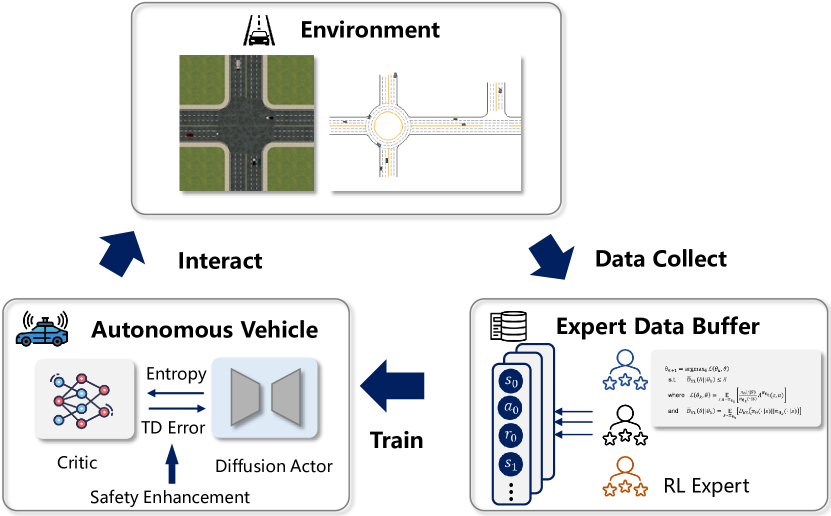
Figure 1: The overall procedure of our work.

II Related Works

II-A Decision-Making of Autonomous Vehicles

The decision-making process is a cornerstone in the functionality of autonomous vehicles (AVs). Traditional approaches in this realm encompass rule-based, game theory-based, and learning-based methodologies. Significantly, with the advent and rapid progression of deep learning and artificial intelligence, learning-based approaches have garnered increasing interest. These methods, particularly reinforcement learning (RL) [10, 11] and large language models (LLM) [12, 13], exhibit formidable and extraordinary learning capacities. They adeptly handle intricate and dynamic environments where conventional rule-based decision-making systems may falter or respond sluggishly [14].

Saxena et al. [10] introduced a pioneering model-free RL strategy, enabling the derivation of a continuous control policy across the AVs’ action spectrum, thus significantly enhancing safety in dense traffic situations. Liu et al. [15] developed a transformer-based model addressing the multi-task decision-making challenges at unregulated intersections. Concurrently, LLMs have also emerged as a focal point in AV decision-making. The Dilu framework [12], integrating a Reasoning and Reflection module, facilitates decision-making grounded in common-sense knowledge and allows for continuous system evolution.

II-B Reinforcement Learning in Safe Decision-Making

In contemporary research, reinforcement learning is recognized as an efficacious learning-based method for sequential decision-making. By optimizing the cumulative reward, RL identifies the optimal action strategy for agents [16], finding applications in domains such as robotic control, gaming, and autonomous vehicles [17]. However, the ’black box’ nature of RL makes the safety of its policy outputs challenging to guarantee.

To augment the safety aspect in RL decision-making, various methodologies have been proposed to incorporate safety layers or regulate the agents’ exploratory processes during training [18, 19]. Safe RL is often conceptualized as a Constrained Markov Decision Process (CMDP) [20], incorporating constraints to mitigate unsafe exploration by the agent. Borkar [21] proposed an actor-critic RL approach for CMDP, employing the envelope theorem from mathematical economics and analyzing primal-dual optimization through a three-time scale process. Berkenkamp et al. [22] developed a safe model-based RL algorithm using Lyapunov functions, ensuring stability under the assumption of a Gaussian process prior.

II-C Applications of the Diffusion Model

The diffusion model has emerged as a potent generative deep-learning tool, utilizing a denoising framework for data generation, with notable success in image generation and data synthesis [5]. Recent studies have applied the diffusion model to sequential decision-making challenges, functioning as a planner [23, 24], policy network [7, 9], and data synthesizer [8, 9].

Diffuser [23] employs the diffusion model for trajectory generation, leveraging offline dataset learning and guided sampling for future trajectory planning. Wang et al. [7] demonstrated the superior performance of a diffusion-model-based policy over traditional Gaussian policies in Q-learning, particularly for offline reinforcement learning. Additionally, to enhance dataset robustness, Lu et al. [8] utilized the diffusion model for data synthesis, learning from both offline and online datasets.

In our study, we posit the diffusion model as a central actor in the decision-making process of autonomous agents, aiming to augment the flexibility and diversity in AV decision-making strategies.

III Preliminaries

III-A Constrained Markov Decision Process (CMDP)

A CMDP is characterized by the tuple $(S,A,R,C,\gamma,\mu)$, where $S$ represents the state space, $A$ denotes the action space, $R:S\times A\rightarrow\mathbb{R}$ is the reward function, and $C:S\times A\rightarrow\mathbb{R}$ signifies the corresponding single-stage cost function. The discount factor is denoted by $\gamma$, and $\mu$ indicates the initial state distribution. We define a policy $\pi$ as a map to from states to a probability distribution over actions, and $\pi(a|s)$ represents the probability of action $a$ based on state $s$.

Our study focuses on a class of stationary policies $\pi_{\theta}$, parameterized by $\theta$. The objective function is framed in terms of the infinite horizon discounted reward criterion: $\mathbb{E}\left[\sum_{t=0}^{\infty}\gamma^{t}R(s_{t},a_{t})\mid s_{0}\sim\mu,a_{t}\sim\pi_{\theta},\forall t\right]$. Similarly, the constraint function is expressed via the infinite horizon discounted cost: $\mathbb{E}\left[\sum_{t=0}^{\infty}\gamma^{t}C(s_{t},a_{t})\mid s_{0}\sim\mu,a_{t}\sim\pi_{\theta},\forall t\right]$. The optimization problem with constraints can be formulated as follows:

$$\max_{\theta}\mathbb{E}\left[\sum_{t=0}^{\infty}\gamma^{t}R(s_{t},a_{t})\mid s_{0}\sim\mu,a_{t}\sim\pi_{\theta},\forall t\right].$$ (1)

$$\ \mbox{s.t.}\ \mathbb{E}\left[\sum_{t=0}^{\infty}\gamma^{t}C(s_{t},a_{t})\mid s_{0}\sim\mu,a_{t}\sim\pi_{\theta},\forall t\right]\leq d.$$

III-B Diffusion Model

Diffusion-based generative model utilizes a parameterized diffusion process to mode the process that how the pure noise is denoised into real data. The process is denoted as $p_{\theta}(x_{0})=\int p(x_{T}){\textstyle\prod_{t=1}^{T}}p_{\theta}(x_{t-1}|x_{t})\,dx_{1:T}$, where $x_{1},\ldots,x_{T}$ serve as latent variables with dimensionality matching that of the data $x_{0}\sim p(x_{0})$. A forward diffusion process incrementally introduces noise to the data $x_{0}\sim q(x_{0})$ across $T$ steps, following a predetermined variance schedule $\beta_{i}$, formalized as

$$q(x_{1:T}\,|\,x_{0})=\prod_{t=1}^{T}q(x_{t}\,|\,x_{t-1})$$ (2)

$$\quad q(x_{t}\,|\,x_{t-1})=\mathcal{N}(x_{t};\sqrt{1-\beta_{t}}x_{t-1},\beta_{t}\mathbf{I}).$$ (3)

The reverse diffusion process is articulated as $p_{\theta}(x_{0:T})=\mathcal{N}(x_{T};\mathbf{0},\mathbf{I})\prod_{t=1}^{T}p_{\theta}(x_{t-1}\,|\,x_{t}),$ and is optimized through the maximization of the evidence lower bound, defined as $\mathbb{E}_{q}[\ln\frac{p_{\theta}(x_{0:T})}{q(x_{1:T}\,|\,x_{0})}]$. Upon completion of training, the sampling from the diffusion model entails initiating from $x_{T}\sim p(x_{T})$ and employing the reverse diffusion chain to transition from $t=T$ to $t=0$.

III-C Lagrangian Methods

In the context of the constrained optimization problem as delineated in Eq.1, the associated Lagrangian can be articulated as:

$$L(\theta,\lambda)=O^{R}(\pi_{\theta})-\lambda(O^{C}(\pi_{\theta})-d)$$ (4)

where $\lambda\in\mathbb{R}^{+}$ denotes the Lagrange multiplier, $O^{R}(\pi_{\theta})=\mathbb{E}\left[\sum_{t=0}^{\infty}\gamma^{t}R(s_{t},a_{t},s_{t+1})\mid s_{0}\sim\mu,a_{t}\sim\pi_{\theta},\forall t\right]$, $O^{C}(\pi_{\theta})=\mathbb{E}\left[\sum_{t=0}^{\infty}\gamma^{t}C(s_{t},a_{t},s_{t+1})\mid s_{0}\sim\mu,a_{t}\sim\pi_{\theta},\forall t\right]$. The objective is to identify a tuple $(\theta^{*},\lambda^{*})$ that represents both the policy and the Lagrange parameter, fulfilling the condition:

$$L(\theta^{*},\lambda^{*})=\max_{\theta}\min_{\lambda}L(\theta,\lambda).$$ (5)

Resolving the max-min problem is tantamount to locating a global optimal saddle point $(\theta^{*},\lambda^{*})$ such that for all $(\theta,\lambda)$, the following inequality is maintained:

$$L(\theta^{*},\lambda)\geq L(\theta^{*},\lambda^{*})\geq L(\theta,\lambda^{*}).$$ (6)

Given that $\theta$ is associated with the parameters of a Deep Neural Network, identifying such a globally optimal saddle point is computationally challenging. Thus, our objective shifts to finding a locally optimal saddle point, satisfying Eq.6 within a defined local neighbourhood $H_{\epsilon_{1},\epsilon_{2}}$:

$$H_{\epsilon_{1},\epsilon_{2}}\stackrel{{\scriptstyle\triangle}}{{=}}\{(\theta,\lambda)|\ \|\theta-\theta^{*}\|\leq\epsilon_{1},\|\lambda-\lambda^{*}\|\leq\epsilon_{2}\}$$ (7)

for some $\epsilon_{1},\epsilon_{2}>0$. Assuming $L(\theta,\lambda)$ is determinable for every $(\theta,\lambda)$ tuple, the gradient search algorithm will be used as to identify a local $(\theta^{*},\lambda^{*})$ pair[25].

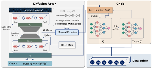
Figure 2: The framework of DDM-Lag algorithm.

IV Methodology

IV-A Framework Overview

In this study, we conceptualize the decision-making process of autonomous vehicles through the lens of a Constrained Markov Decision Process. As shown in Fig.2, our framework introduces an Actor-Critic architecture, pivotal for the exploration and learning of agent policies. The policy network $\pi_{\theta}$, coupled with the Q-network $Q_{\phi}$ and $Q_{\psi}$ are set in this framework. Given the demonstrated efficacy of diffusion models in dataset integration and training robustness, our approach is anchored in a diffusion model-based actor, signified by the policy network $\pi_{\theta}$, and MLP-based Critic networks. Within the realms of the CMDP, our primary objective is the maximization of cumulative rewards, tempered by the imperative of incorporating safety losses as critical constraints in our optimization framework. We tackle the intricate optimization challenges via the Lagrangian relaxation method, employing a PID controller for the dynamic adjustment of Lagrange multipliers.

IV-B Diffusion-based Actor

At any given moment, an autonomous vehicle must make decisions a based on its current state s, expressed as $\pi_{\theta}(a\,|\,s)$. We model the actor’s policy using the reverse process of conditional diffusion models: $\textstyle\pi_{\theta}(a\,|\,s)=p_{\theta}(a^{0:N}\,|\,s)={\mathcal{N}}(a^{N};\mathbf{0},{\bm{I}})\prod_{i=1}^{N}p_{\theta}(a^{i-1}\,|\,a^{i},s)$ where $a^{0}$, the end sample of the reverse chain, represents the action executed and evaluated. This work distinguishes between two types of timesteps: diffusion timesteps denoted by superscripts $i\in\{1,\dots,N\}$ and trajectory timesteps denoted by subscripts $t\in\{1,\dots,T\}$. In this context, autonomous vehicles and agents are synonymous and not distinctly defined. The conditional distribution $p_{\theta}(a^{i-1}\,|\,a^{i},s)$ can be modeled as a Gaussian distribution ${\mathcal{N}}(a^{i-1};\mu_{\theta}(a^{i},s,i),{\bm{\Sigma}}_{\theta}(a^{i},s,i))$. Following  [26], we parameterize $p_{\theta}(a^{i-1}\,|\,a^{i},s)$ as a noise prediction model, fixing the covariance matrix as ${\bm{\Sigma}}_{\theta}(a^{i},s,i)=\beta_{i}{\bm{I}}$, and constructing the mean as:

$$\mu_{\theta}(a^{i},s,i)=\frac{1}{\sqrt{\alpha_{i}}}\big{(}a^{i}-\frac{\beta_{i}}{\sqrt{1-\bar{\alpha}_{i}}}{\bm{\epsilon}}_{\theta}(a^{i},s,i)\big{)}$$

. The reverse diffusion chain, parameterized by $\theta$, is sampled as:

$$\textstyle a^{i-1}\,|\,a^{i}=\frac{a^{i}}{\sqrt{\alpha_{i}}}-\frac{\beta_{i}}{\sqrt{\alpha_{i}(1-\bar{\alpha}_{i})}}{\bm{\epsilon}}_{\theta}(a^{i},s,i)+\sqrt{\beta_{i}}{\bm{\epsilon}},$$ (8)

$$~{}~{}{\bm{\epsilon}}\sim\mathcal{N}(\mathbf{0},{\bm{I}}),~{}~{}\text{for }i=N,\ldots,1.$$

When $i=1$, ${\bm{\epsilon}}$ is set to 0 to enhance sampling quality. We adopt the simplified objective proposed by  [26] to train our conditional ${\bm{\epsilon}}$-model via:

$$\mathcal{L}_{d}(\theta)=\mathbb{E}_{i\sim\mathcal{U},{\bm{\epsilon}}\sim\mathcal{N}(\mathbf{0},{\bm{I}}),(s,a)\sim\mathcal{D}}$$ (9)

$$\left[||{\bm{\epsilon}}-{\bm{\epsilon}}_{\theta}(\sqrt{\bar{\alpha}_{i}}a+\sqrt{1-\bar{\alpha}_{i}}{\bm{\epsilon}},s,i)||^{2}\right]$$

where $\mathcal{U}$ is a uniform distribution over the discrete set $\{1,\dots,N\}$ and $\mathcal{D}$ denotes the offline dataset.

IV-C Policy Learning from Exploration

During training, the Actor-Critic framework alternates between policy evaluation and policy improvement in each iteration, dynamically updating the Critic $Q_{\phi}$ and the Actor $\pi_{\theta}$. In the policy evaluation phase, we update the estimated Q-function by minimizing the L2 norm of the entropy-regularized TD error:

$$y(r_{t},s_{t+1})=r_{t}+\gamma\mathbb{E}_{a_{t+1}\sim\pi_{\theta}(\cdot|s_{t+1})}\ [Q_{\phi^{\prime}}(s_{t+1},a_{t+1})]$$ (10)

$$-\alpha\log\pi_{\theta}(a_{t+1}|s_{t+1})]$$

$$L_{Q}(\phi)=\cfrac{1}{2}\mathbb{E}_{(s_{t},a_{t},r_{t},s_{t+1})\sim\mathcal{D}}[y(r_{t},s_{t+1})-Q_{{\phi}}(s_{t},a_{t})]^{2}.$$ (11)

where $\phi^{\prime}$ is the parameter of the target network $Q_{\phi^{\prime}}$, and $\alpha$ is the temperature parameter.

In the policy improvement phase, for the diffusion-based actor $\pi_{\theta}$, our update target function comprises two parts: the policy regularization loss term $\mathcal{L}_{d}(\theta)$ and the policy improvement objective term $\mathcal{L}_{q}(\theta)$. The policy regularization loss term $\mathcal{L}_{d}(\theta)$, equivalent to behavior cloning loss, is utilized for learning expert prior knowledge from human expert demonstration data. However, as it is challenging to surpass expert performance solely with this, we introduce a Q-function-based policy improvement objective term $\mathcal{L}_{q}(\theta)$ during training, guiding the diffusion model to prioritize sampling high-value actions. Consequently, our policy learning objective function is expressed as:

$$\pi=\operatorname*{arg\,min}_{\pi_{\theta}}\mathcal{L}(\theta)=\mathcal{L}_{d}(\theta)+\mathcal{L}_{q}(\theta)$$ (12)

$$=\mathcal{L}_{d}(\theta)-\alpha\cdot\mathbb{E}_{s\sim\mathcal{D},a^{0}\sim\pi_{\theta}}\left[Q_{\phi}(s,a^{0})\right].$$

$a^{0}$ is reparameterized by Eq. 8, allowing the Q-value function gradient with respect to the action to propagate backward through the entire diffusion chain.

IV-D Safety Enhancement with Constrained Optimization

Due to the inherent randomness in the Actor’s exploratory process, ensuring the safety of its actions is a significant challenge, particularly in autonomous vehicle decision-making. To enhance safety in the learning and policy updating processes, we incorporate safety constraints into the policy update process, treating the original problem as a constrained optimization issue. The safety cost function is defined as follows:

$$C=\omega_{1}c_{1}+\omega_{2}c_{2}+\omega_{3}c_{3}$$ (13)

where $c_{1}$, $c_{2}$ and $c_{3}$ are the penalty for the condition: out of road, crashing with other vehicles, crashing with other objects, respectively.

Then we apply the Lagrangian method to this optimization process. The entire optimization problem becomes:

$$\theta^{*}=\mathop{\arg\max}_{\theta}\ \mathop{\min}_{\lambda\geq 0}\mathbb{E}\{(\sum_{t=0}\gamma^{t}R_{t})-\lambda[(\sum_{t=0}\gamma^{t}\hat{C}_{t})-C]\}$$ (14)

Here, $\theta$ and $\lambda$ are updated through policy gradient ascent and stochastic gradient descent (SGD)[27]. We then introduce a safety-assessing Critic $Q_{\psi}^{C}$ to estimate the cumulative safety constraint value $\sum_{t^{\prime}=t}\gamma^{(t-t^{\prime})}C_{t}$. With the reward replaced by the safety constrain, the safety-critic network can be optimized by Eq.11. For the actor $\pi_{\theta}$, the safety constraint violation minimization objective can be written as:

$$L_{q}^{\lambda}(\theta)=\mathbb{E}_{s_{t}\sim\mathcal{D},a_{t}\sim\pi_{\theta}(\cdot|s_{t})}[Q^{C}_{\psi}(s_{t},a_{t})-C]$$ (15)

Now, by combining the original policy improvement objective Eq.12 and the safety constraint minimization optimization objective Eq.15, we derive our final policy update objective:

$$\pi=\operatorname*{arg\,min}_{\pi_{\theta}}\mathcal{L}(\theta)=\mathcal{L}_{d}(\theta)+\mathcal{L}_{q}(\theta)+\lambda\mathcal{L}_{q}^{\lambda}(\theta)$$ (16)

However, directly optimizing the Lagrangian dual during policy updates can lead to oscillation and overshooting, thus affecting the stability of policy updates. From a control theory perspective, the multiplier update represents an integral control. Therefore, following [28], we introduce proportional and derivative control to update the Lagrangian multiplier, which can reduce oscillation and lower the degree of action violation. Specifically, we use a PID controller to update $\lambda$, as follows:

$$\lambda\leftarrow K_{p}\delta+K_{i}\int_{i=1}^{k}\delta di+K_{d}\cfrac{\delta}{di},$$ (17)

$$\delta=\mathbb{E}_{\tau}[\sum_{t=0}\hat{c}_{t}]-C$$

where we denote the training iteration as $i$, and $K_{p}$, $K_{i}$, $K_{d}$ are the hyper-parameters. Optimizing $\lambda$ with Eq. 14 reduces to the proportional term in Eq. 17, while the integral and derivative terms compensate for the accumulated error and overshoot in the intervention occurrence. The whole training procedure of DDM-Lag is summarized in Algorithm 1.

Inputs : Transition mini-batch $\mathcal{B}$, Offline Dataset $\mathcal{D}$

Outputs : Updated policy and critics: $\theta^{\prime}$,$\phi^{\prime}$,$\psi^{\prime}$

1   Initialize policy network $\pi_{\theta}$; critic networks $Q_{\phi}$;cost critic networks $Q^{C}_{\psi}$; and their target networks $\pi_{\theta^{\prime}}$, $Q_{\phi^{\prime}}$, $Q^{C}_{\psi^{\prime}}$;

2 for $Epoch=1$ to $M$ do

3       Sample transition mini-batch $\mathcal{B}=\{(s_{t},a_{t},r_{t},s_{t+1})\}\sim\mathcal{D}$;

4       Sample $a_{t+1}^{0}\sim\pi_{\theta^{\prime}}(a_{t+1}|s_{t+1})$ by Eq. 8;

5       Update $Q_{\phi}$ and $Q_{\psi}$ by Eq.11;

6      

7      Policy learning:

8       Sample $a_{t}^{0}\sim\pi_{\theta}(a_{t}|s_{t})$ by Eq.8;

9       Update policy by minimizing Eq.16;

10       Update target networks:

11       $\theta^{\prime}=\rho\theta^{\prime}+(1-\rho)\theta$,

12       $\phi^{\prime}=\rho\phi^{\prime}+(1-\rho)\phi$,

13       $\psi^{\prime}=\rho\psi^{\prime}+(1-\rho)\psi$,

14       Update lagrange multiplier $\lambda$ by Eq.17

15 end for

Algorithm 1 Diffusion Decision Model with Safe Enhancement

V Experiment and Evaluation

In this section, the detailed information of the simulation environment and our models will be introduced. Sequently, the experiments results are analyzed.

V-A Experiments and Baselines

Environments. We conducted our experiments, including data collection, model training, and testing, in the MetaDrive Simulator [29], which is based on OpenAI Gym Environment and allows for the creation of various traffic scenarios. Our study involves two types of combined traffic scenarios. The first scenario comprises a straight road and a curved road, designed to test the fundamental decision-making skills required for autonomous driving. The second scenario features a mix of unsignalized intersections and roundabouts, introducing more complex interactions and decision-making challenges for autonomous vehicles. Fig.3 illustrates these scenarios. Additionally, we varied the traffic flow density in each scenario, setting it at 0.1 for low-density traffic and 0.2 for high-density traffic, to modulate the complexity of the scenes.

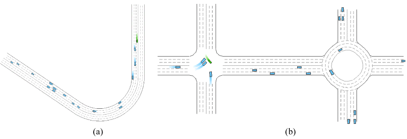
Figure 3: The two kinds of mixed scenario used for traning and testing our method, (a) scenario 1, (b) scenario 2.

Dataset Collection. An offline dataset of expert-level data is crucial for training our diffusion model. As depicted in Fig.1, we used a Soft Actor-Critic (SAC) with Lagrangian[30] as the expert agent for environment exploration and data collection. This expert agent gathered data, including trajectories and reward feedback from diverse environments. This data was stored in a buffer to create the offline dataset. For each scenario, with varying difficulty levels and traffic densities, we collected $10K$ trajectories using the expert agent.

Baselines. Our study compares three baseline methods, each known for their effectiveness in different tasks. These methods include classic behavior cloning (BC), Batch-Constrained deep Q-learning (BCQL)  [31], and Deep Q-learning with a diffusion policy (Diffusion Q-learning).

V-B Implementation Details

For each model,the training timesteps is $20K$ , batch size is 512 and the cost uplimit $C$ for the cost function Eq. 13 is set as 10. Our diffusion model is built based on a 3-layer MLP with 256 hidden units for all networks. As for BCQ and Diffusion Q-learning baseline, the policy network is set as same as our diffusion actor. For the diffusion model, the number of diffusion steps $N$ is set as 5. The $K_{p}$, $K_{i}$ and $K_{d}$ for the PID controller are set as 0.1,0.003,0.001, respectively. In the safety cost function, $c_{1}=1.0$, $c_{2}=5.0$ and $c_{3}=5.0$. The coefficient of each cost function term is set as 1. Other parameters are shown in Tab.I. All experiments are conducted in a computation platform with Intel Xeon Silver 4214R CPU and NVIDIA GeForce RTX 3090 GPU.

TABLE I: The hyperparameter setting of our work

Symbol	Definition	Value
$B_{s}$	Batch Size	256
$l_{a}$	actor learning rate	0.001
$l_{c}$	critic learning rate	0.99
$\lambda$	Weight of the Lagrangian term	0.75
$\gamma$	Discount factor for the reward	0.99
$\tau$	Soft update coefficient of the target network	0.005

V-C Results Analysis

V-C1 Model Training

During the training of our model, the reward and running length curves for the diffusion actor are illustrated in Fig. 4(a) and (b), respectively. These figures demonstrate that our model can learn and converge steadily.

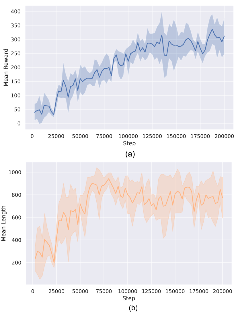
Figure 4: The model performance during training, (a)the reward curve,(b) the running length curve.

V-C2 Performance Evaluation

We assessed the performance of our method alongside several baseline algorithms in two scenarios with different traffic densities. Our evaluation criteria included security violation cost, security decision-making time, and an overall performance score. The latter is a comprehensive metric we developed, normalizing security violation cost and efficiency. Animations demonstrating cases from DDM-Lag can be accessed at the site.

Safety Analysis. In autonomous driving, safety is paramount. Tab.II details the safety performance of different models. Lower safety costs indicate fewer risky decisions and higher algorithmic safety. On average, BC and Diffusion QL algorithm recorded the highest safety costs at 21.319 and 23.247, respectively. BCQL algorithm showed improved safety, averaging a cost of 18.346, thanks to its safety constraints. Our proposed DDM-Lag algorithm excelled in safety, with an average cost of just 0.841, significantly outperforming other algorithms.

Running Length Analysis. As shown in Tab.III, we also examined the running length of various algorithms. Shorter runs, halted by collisions or other failures, indicate less durable and safe decision-making. The DDM-Lag method, benefiting from its safety advantages, achieved an impressive average explored timestep of 636.806. In contrast, BC and Diffusion QL algorithm had similar performances at 344.481 and 340.779, respectively, while BCQL algorithm lagged at 225.576.

Comprehensive Performance. To further analyze the safety and efficiency of various algorithms, we employed two metrics: Time to Collision (TTC) and Post Encroachment Time (PET) to evaluate the performance of AV in Scenarios 1 and 2. We calculated the minimum TTC and average PET, along with the average speed of the AVs, with results presented in Tab.IV. In Scenario 1, the Diffusion QL algorithm exhibited the smallest TTC and highest average speed, leading to poorer safety performance. The BC and BCQL algorithms performed marginally better; however, the BC algorithm showed a lower average speed. In contrast, our DDM-Lag method maintained a significantly higher speed than the BC algorithm while ensuring a larger TTC, demonstrating its advantage in driving efficiency. In Scenario 2, the BCQL algorithm had the smallest PET and highest average speed, resulting in the highest driving risk and poorest safety performance. The BC algorithm showed the largest PET but at the lowest average speed, indicative of overly conservative driving behavior. Meanwhile, both the Diffusion QL and our DDM-Lag algorithm exhibited a better balance between safety and efficiency.

Furthermore, based on the comprehensive performance in terms of safety and efficiency, we calculated comprehensive scores for the different algorithms, as shown in Table V. The BC and Diffusion QL algorithms were closely matched with scores of 32.316 and 31.753, respectively. The BCQL algorithm scored 20.723. Notably, our DDM-Lag method achieved the highest score of 63.597, highlighting the effectiveness of our approach.

Overall, compared to other algorithms, DDM-Lag demonstrates superior ability to balance safety and efficiency across various scenarios, thereby yielding better decision-making performance.

TABLE II: The Average Safety Cost of Different Algorithms in Testing.

Task	BC	BCQL	Diffusion QL	DDM-Lag
Sce.1-Den.1	13.654	11.293	8.919	0.720
Sce.1-Den.2	30.283	26.721	31.146	0.874
Sce.2-Den.1	18.625	9.26	22.825	0.789
Sce.2-Den.2	22.712	26.109	30.096	0.980
Average	21.319	18.346	23.247	0.841

TABLE III: The Average Running Length of Different Algorithms in Testing.

Task	BC	BCQL	Diffusion QL	DDM-Lag
Sce.1-Den.1	313.658	323.409	370.836	643.603
Sce.1-Den.2	288.653	107.381	153.725	522.458
Sce.2-Den.1	412.955	398.6	437.034	712.253
Sce.2-Den.2	362.658	72.913	401.521	668.911
Average	344.481	225.576	340.779	638.806

TABLE IV: Performance Evaluation Results of Different Algorithms.

	BC	BCQL	Diffusion QL	DDM-Lag
TTC-Sce.1	2.71	1.89	0.48	2.4
Ave Speed(m/s)-Sce.1	6.32	13.6	22.98	12.26
PET-Sce.2	5.04	7.97	4.29	3.34
Ave Speed(m/s)-Sce.2	5.22	30.79	9.05	8.2

TABLE V: The Comprehensive Scores of Different Algorithms in Testing.

Task	BC	BCQL	Diffusion QL	DDM-Lag
Sce.1-Den.1	30.000	31.212	36.192	64.288
Sce.1-Den.2	25.837	8.066	12.258	52.158
Sce.2-Den.1	39.433	38.934	41.421	71.146
Sce.2-Den.2	33.995	4.680	37.143	66.793
Average	32.316	20.723	31.753	63.597

VI Conclusion

Decision-making processes are fundamental to the operational integrity and safety of autonomous vehicles (AVs). Contemporary data-driven decision-making algorithms in this domain exhibit a discernible potential for enhancements.

In this study, we introduce DDM-Lag, a diffusion-based decision-making model for AVs, distinctively augmented with a safety optimization constraint. A key point in our approach involves the integration of safety constraints within CMDP to ensure a secure action exploration framework. Furthermore, we employ a policy optimization method based on Lagrangian relaxation to facilitate comprehensive updates of the policy learning process. The efficacy of the DDM-Lag model is evaluated in different driving tasks. Comparative analysis with baseline methods reveals that our model demonstrates enhanced performance, particularly in the aspects of safety and comprehensive operational effectiveness.

Looking ahead, we aim to further refine the inference efficiency of the DDM-Lag model by fine-tuning its hyperparameters. We also plan to explore and integrate additional safety enhancement methodologies to elevate the safety performance of our model. Moreover, the adaptability and robustness of our model will be subjected to further scrutiny through its application in an expanded array of scenarios and tasks.

APPENDIX

The state space, action space, and reward function in our experiment are described in detail in the appendix.

VI-A State Space

In our study, the state input of the autonomous vehicle comprises four main components. The first component is the ego vehicle’s own state, including its position $[x_{\text{ego}},y_{\text{ego}}]$, velocity $[v_{x_{\text{ego}}},v_{y_{\text{ego}}}]$, steering angle [heading], and distance from the road boundary [$dis_{bound}$]. The second component is navigation information, for which we calculate a route from the origin to the destination and generate a set of checkpoints along the route at predetermined intervals, providing the relative distance and direction to the next checkpoint as navigation data. The third component consists of a 240-dimensional vector, characterizing the vehicle’s surrounding environment in a manner akin to LiDAR point clouds. The LiDAR sensor scans the environment in a 360-degree horizontal field of view using 240 lasers, with a maximum detection radius of 50 meters and a horizontal resolution of 1.5 degrees. The final component includes the state of surrounding vehicles, such as their position and velocity information, acquired through V2X communication.

VI-B Action Space

We utilize two normalized actions to control the lateral and longitudinal motion of the target vehicle, denoted as $\mathbf{a}=[a_{1},a_{2}]^{T}\in(0,1)$. These normalized actions are subsequently translated into low-level continuous control commands: steering $u_{s}$, acceleration $u_{a}$, and brake signal $u_{b}$ as follows:

$$u_{s}=S_{\text{max}}\cdot a_{1}$$ (18)

$$u_{a}=F_{\text{max}}\cdot\max\{0,a_{2}\}$$

$$u_{b}=-B_{\text{max}}\cdot\min\{0,a_{2}\}$$

where $S_{\text{max}}$ represents the maximum steering angle, $F_{\text{max}}$ the maximum engine force, and $B_{\text{max}}$ the maximum braking force.

VI-C Reward Function

The reward function plays a crucial role in optimizing the agent’s performance. In our study, we define the reward function as:

$$R=\omega^{\prime}_{1}r_{dis}+\omega^{\prime}_{2}r_{v}+\omega^{\prime}_{3}r_{s}-\omega^{\prime}_{4}r_{c}$$ (19)

The components include $r_{dis}$ for the reward based on distance covered, $r_{v}$ for the speed reward, $r_{s}$ for the terminal reward, and $r_{c}$ as a penalty for any dangerous actions taken by the agent, which is equivalent to the cost penalty function Eq.13.

In our experiment, we set the following values for the reward function: $r_{dis}=1$, $r_{v}=0.1$, $r_{s}=10$, $r_{c1}=5.0$, $r_{c2}=5.0$ and $r_{c3}=5.0$. The coefficient of each reward term is set as 1.

References

- [1] Z. Wang, C. Lv, and F.-Y. Wang, “A new era of intelligent vehicles and intelligent transportation systems: Digital twins and parallel intelligence,” IEEE Transactions on Intelligent Vehicles, 2023.
- [2] P. Hang, Y. Zhang, N. de Boer, and C. Lv, “Conflict resolution for connected automated vehicles at unsignalized roundabouts considering personalized driving behaviours,” Green Energy and Intelligent Transportation, vol. 1, no. 1, p. 100003, 2022.
- [3] J. Liu, D. Zhou, P. Hang, Y. Ni, and J. Sun, “Towards socially responsive autonomous vehicles: A reinforcement learning framework with driving priors and coordination awareness,” IEEE Transactions on Intelligent Vehicles, 2023.
- [4] B. R. Kiran, I. Sobh, V. Talpaert, P. Mannion, A. A. Al Sallab, S. Yogamani, and P. Pérez, “Deep reinforcement learning for autonomous driving: A survey,” IEEE Transactions on Intelligent Transportation Systems, vol. 23, no. 6, pp. 4909–4926, 2021.
- [5] F.-A. Croitoru, V. Hondru, R. T. Ionescu, and M. Shah, “Diffusion models in vision: A survey,” IEEE Transactions on Pattern Analysis and Machine Intelligence, 2023.
- [6] L. Yang, Z. Zhang, Y. Song, S. Hong, R. Xu, Y. Zhao, W. Zhang, B. Cui, and M.-H. Yang, “Diffusion models: A comprehensive survey of methods and applications,” ACM Computing Surveys, vol. 56, no. 4, pp. 1–39, 2023.
- [7] Z. Wang, J. J. Hunt, and M. Zhou, “Diffusion policies as an expressive policy class for offline reinforcement learning,” arXiv preprint arXiv:2208.06193, 2022.
- [8] C. Lu, P. J. Ball, and J. Parker-Holder, “Synthetic experience replay,” arXiv preprint arXiv:2303.06614, 2023.
- [9] H. He, C. Bai, K. Xu, Z. Yang, W. Zhang, D. Wang, B. Zhao, and X. Li, “Diffusion model is an effective planner and data synthesizer for multi-task reinforcement learning,” arXiv preprint arXiv:2305.18459, 2023.
- [10] D. M. Saxena, S. Bae, A. Nakhaei, K. Fujimura, and M. Likhachev, “Driving in dense traffic with model-free reinforcement learning,” in 2020 IEEE International Conference on Robotics and Automation (ICRA). IEEE, 2020, pp. 5385–5392.
- [11] G. Li, S. Li, S. Li, Y. Qin, D. Cao, X. Qu, and B. Cheng, “Deep reinforcement learning enabled decision-making for autonomous driving at intersections,” Automotive Innovation, vol. 3, pp. 374–385, 2020.
- [12] L. Wen, D. Fu, X. Li, X. Cai, T. Ma, P. Cai, M. Dou, B. Shi, L. He, and Y. Qiao, “Dilu: A knowledge-driven approach to autonomous driving with large language models,” arXiv preprint arXiv:2309.16292, 2023.
- [13] L. Chen, O. Sinavski, J. Hünermann, A. Karnsund, A. J. Willmott, D. Birch, D. Maund, and J. Shotton, “Driving with llms: Fusing object-level vector modality for explainable autonomous driving,” arXiv preprint arXiv:2310.01957, 2023.
- [14] W. Schwarting, J. Alonso-Mora, and D. Rus, “Planning and decision-making for autonomous vehicles,” Annual Review of Control, Robotics, and Autonomous Systems, vol. 1, pp. 187–210, 2018.
- [15] J. Liu, P. Hang, J. Wang, J. Sun et al., “Mtd-gpt: A multi-task decision-making gpt model for autonomous driving at unsignalized intersections,” arXiv preprint arXiv:2307.16118, 2023.
- [16] B. B. Elallid, N. Benamar, A. S. Hafid, T. Rachidi, and N. Mrani, “A comprehensive survey on the application of deep and reinforcement learning approaches in autonomous driving,” Journal of King Saud University-Computer and Information Sciences, vol. 34, no. 9, pp. 7366–7390, 2022.
- [17] H.-n. Wang, N. Liu, Y.-y. Zhang, D.-w. Feng, F. Huang, D.-s. Li, and Y.-m. Zhang, “Deep reinforcement learning: a survey,” Frontiers of Information Technology & Electronic Engineering, vol. 21, no. 12, pp. 1726–1744, 2020.
- [18] S. Gu, L. Yang, Y. Du, G. Chen, F. Walter, J. Wang, Y. Yang, and A. Knoll, “A review of safe reinforcement learning: Methods, theory and applications,” arXiv preprint arXiv:2205.10330, 2022.
- [19] J. Garcıa and F. Fernández, “A comprehensive survey on safe reinforcement learning,” Journal of Machine Learning Research, vol. 16, no. 1, pp. 1437–1480, 2015.
- [20] E. Altman, Constrained Markov decision processes. Routledge, 2021.
- [21] V. S. Borkar, “An actor-critic algorithm for constrained markov decision processes,” Systems & control letters, vol. 54, no. 3, pp. 207–213, 2005.
- [22] F. Berkenkamp, M. Turchetta, A. Schoellig, and A. Krause, “Safe model-based reinforcement learning with stability guarantees,” Advances in neural information processing systems, vol. 30, 2017.
- [23] M. Janner, Y. Du, J. B. Tenenbaum, and S. Levine, “Planning with diffusion for flexible behavior synthesis,” arXiv preprint arXiv:2205.09991, 2022.
- [24] A. Ajay, Y. Du, A. Gupta, J. Tenenbaum, T. Jaakkola, and P. Agrawal, “Is conditional generative modeling all you need for decision-making?” arXiv preprint arXiv:2211.15657, 2022.
- [25] M. Andrychowicz, M. Denil, S. Gomez, M. W. Hoffman, D. Pfau, T. Schaul, B. Shillingford, and N. De Freitas, “Learning to learn by gradient descent by gradient descent,” Advances in neural information processing systems, vol. 29, 2016.
- [26] J. Ho, A. Jain, and P. Abbeel, “Denoising diffusion probabilistic models,” Advances in neural information processing systems, vol. 33, pp. 6840–6851, 2020.
- [27] S.-i. Amari, “Backpropagation and stochastic gradient descent method,” Neurocomputing, vol. 5, no. 4-5, pp. 185–196, 1993.
- [28] A. Stooke, J. Achiam, and P. Abbeel, “Responsive safety in reinforcement learning by pid lagrangian methods,” in International Conference on Machine Learning. PMLR, 2020, pp. 9133–9143.
- [29] Q. Li, Z. Peng, L. Feng, Q. Zhang, Z. Xue, and B. Zhou, “Metadrive: Composing diverse driving scenarios for generalizable reinforcement learning,” IEEE transactions on pattern analysis and machine intelligence, vol. 45, no. 3, pp. 3461–3475, 2022.
- [30] S. Ha, P. Xu, Z. Tan, S. Levine, and J. Tan, “Learning to walk in the real world with minimal human effort,” arXiv preprint arXiv:2002.08550, 2020.
- [31] S. Fujimoto, D. Meger, and D. Precup, “Off-policy deep reinforcement learning without exploration,” in International conference on machine learning. PMLR, 2019, pp. 2052–2062.