False Discovery Rate and Localizing Power

Abstract

False discovery rate (FDR) is commonly used for correction for multiple testing in neuroimaging studies. However, when using two-tailed tests, making directional inferences about the results can lead to vastly inflated error rate, even approaching 100% in some cases. This happens because FDR only provides weak control over the error rate, meaning that the proportion of error is guaranteed only globally over all tests, not within subsets, such as among those in only one or another direction. Here we consider and evaluate different strategies for FDR control with two-tailed tests, using both synthetic and real imaging data. Approaches that separate the tests by direction of the hypothesis test, or by the direction of the resulting test statistic, more properly control the directional error rate and preserve FDR benefits, albeit with a doubled risk of errors under complete absence of signal. Strategies that combine tests in both directions, or that use simple two-tailed p-values, can lead to invalid directional conclusions, even if these tests remain globally valid. To enable valid thresholding for directional inference, we suggest that imaging software should allow the possibility that the user sets asymmetrical thresholds for the two sides of the statistical map. While FDR continues to be a valid, powerful procedure for multiple testing correction, care is needed when making directional inferences for two-tailed tests, or more broadly, when making any localized inference.

1 Introduction

In the context of the multiple testing problem, control over the false discovery rate (fdr) provides an alternative to the control over the familywise error rate (fwer): while fwer refers to the chance of even one type i (false positive) error is committed in a set (family) of statistical tests, fdr refers to the proportion of such errors among tests for which the null hypothesis has been rejected, that is, the proportion of false discoveries among all discoveries. These topics have been extensively covered in the literature; for an early review of the multiple testing problem in brain imaging, see Nichols and Hayasaka (2003); for an overview of the development of fdr, see Benjamini and Hochberg (2000); for its introduction to neuroimaging, see Genovese et al. (2002); for a critique, see Chumbley and Friston (2009); for a discussion of various fdr approaches, see Korthauer et al. (2019). Methods for fwer correction in brain imaging are typically based on the random field theory (rft – Worsley et al., 1996, 2004), permutation tests (Holmes et al., 1996; Nichols and Holmes, 2002; Winkler et al., 2014), Monte Carlo simulations (Poline and Mazoyer, 1993; Forman et al., 1995; Cox, 1996) and occasionally, the method by Bonferroni (1936).

Two hallmarks of most neuroimaging studies are that they can involve thousands of statistical tests, and that one can reasonably expect effects to be observed on both directions for many of these. Controlling the fdr aims to provide more power than fwer when many tests are expected to show true effects. This benefit has seen fdr widely adopted in neuroimaging. However, the behavior of fdr when signal manifests in positive direction for some tests, and negative for others, has received little attention. We demonstrate that merely applying fdr does not provide optimal sensitivity when the researcher wishes to make inferences about the direction after using two-tailed tests, and can lead to invalid conclusions in cases of effects asymmetrically distributed throughout the tests.

In this note we revisit the use of fdr in brain imaging, discuss interpretation for two-tailed tests in the light of statistical properties of fdr-controlling procedures, and propose methods that can be considered to address issues that emerge when fdr is used with two-tailed tests. We also bring attention to the fdr approach proposed by Benjamini et al. (2006), which is more powerful than the one originally proposed by Benjamini and Hochberg (1995), and which has seldom been used in brain imaging. We also offer a method for p-value adjustment using this more powerful procedure.

2 Theory

Consider a number $V$ of voxels (or vertices, or edges, or faces) of an image representation of the brain. For each, a null hypotheses $\mathcal{H}_{1}$, $\ldots$, $\mathcal{H}_{V}$ is tested, and a corresponding p-value $p_{1}$, $\ldots$, $p_{V}$ is computed. Each p-value can be considered “significant” if equal or below some pre-defined test level $\alpha$ (typically, $\alpha$ $=$ $0.05$). Simply comparing each p-value to $\alpha$ leads to many of them to be spuriously considered significant, even if all null hypotheses are true; for example, if $\alpha$ $=$ $0.05$, 5% of the tests will are expected to be found as significant even if no effect is present in any of them.

One could address this multiple testing problem by choosing a more stringent test level. For example, $\alpha$ could be chosen such that it refers not to errors in each individual test, but to any error in the whole set of tests performed. If all tests are independent, this more stringent level could be computed using the Šidák correction: $\alpha^{\text{\v{S}id\'{a}k}}=1-(1-\alpha)^{1/V}$. Before the computer era, finding the arbitrary root of a number was time-consuming and impractical, particularly for high-degree roots. A simpler method for choosing the test level that does not require complex computations, even if slightly more conservative than that of Šidák, was given by Bonferroni (1936) (apud Heyde and Seneta, 2001): $\alpha^{\text{Bonf.}}=\alpha/V$. Bonferroni and Šidák methods control the chance that any test will be found as significant among a set of tests, i.e., they control the fwer. Both assume that the tests are independent one from another; if not independent (as typically in brain imaging), both methods are remarkably conservative.

Regardless of the degree of dependency among tests, it may be the case that, faced with the task of screening many such tests, a researcher may be willing to tolerate a small amount of them to be incorrectly declared significant (false discoveries), as long as a great majority of tests are correctly declared as such (true discoveries), and the errors are limited. In other words, the researcher may be willing to accept some false discoveries as long as their proportion over all discoveries does not spill over some pre-defined threshold $q$ (often $q$ $=$ $0.05$). Controlling this proportion is the essence of fdr approaches.

2.1 The basic fdr procedure: bh

Control over the fdr can be achieved with the procedure introduced by Benjamini and Hochberg (1995) (bh): let $p_{(1)}\leqslant\ldots\leqslant p_{(V)}$ be their ordered p-values. Find the largest index $i$ for which:

$$p_{(i)}\leqslant\frac{iq}{V}$$ (1)

where $q$ is the upper limit on the proportion of false discoveries that the researcher is willing to tolerate. Then reject all null hypotheses that have p-values smaller than or equal to that critical $p_{(i)}$. Graphically, one would lay the ordered p-values in a Cartesian plane that has as horizontal axis the index $i$; draw a line with slope $q/V$ passing through the origin, then reject all tests whose ordered p-values lie to the left of the highest p-value at or below that line (Figure 1, upper-left panel).

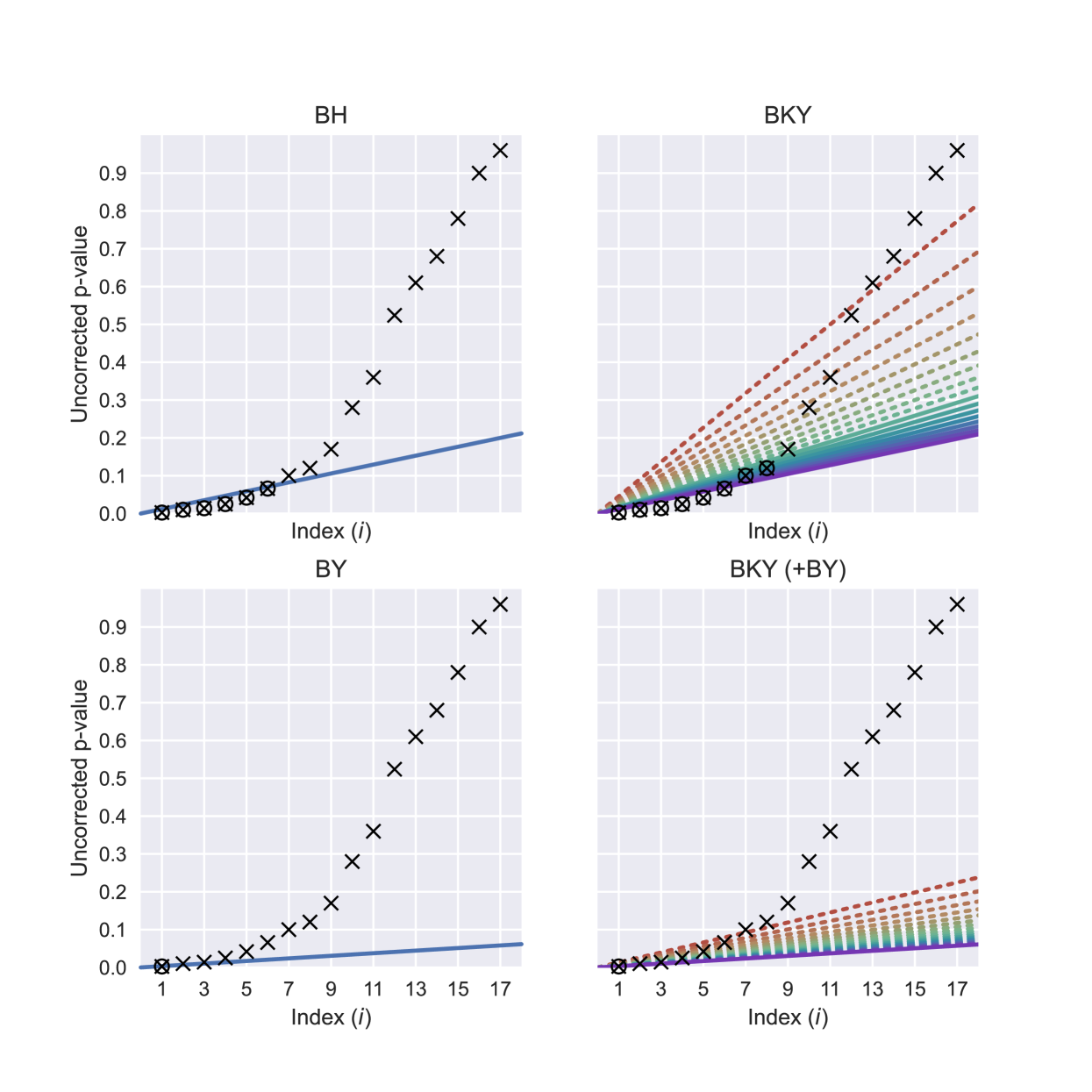
Figure 1: Comparison of fdr correction methods, for $q=0.20$. Each symbol $\boldsymbol{\times}$ represents an uncorrected p-value; these are placed in ascending order ($i$); the p-values considered significant according to the respective method are surrounded by a circle $\boldsymbol{\otimes}$. In bh, p-values smaller than or equal to the highest p-value below a single inclined threshold (blue line) are declared significant. In bky, the thresholds themselves are adaptive: their inclination increases for larger p-values (colored lines), making it easier to detect significant p-values, provided that smaller ones are also found significant (for clarity, we show in dashed lines the thresholds for tests considered not significant). In by, the bh threshold line is scaled down by a constant factor, becoming less inclined (more conservative); the same principle used in by can be applied to bky.
The p-values used in this example are: {0.0026, 0.01, 0.014, 0.025, 0.042, 0.066, 0.1, 0.12, 0.17, 0.28, 0.36, 0.524, 0.61, 0.68, 0.78, 0.9, 0.96}.

When the tests are independent, the bh procedure controls the fdr at the level $qV_{0}/V$, where $V_{0}$ is the (unknown) number of true null hypotheses. However, complete independence is not strictly necessary: it is sufficient for tests to exhibit a form of dependence that has been termed positive regression dependency on subsets (prds). prds means that, for a set of tests that are positively dependent, the dependence is the same or stronger within arbitrarily defined subsets where the null hypothesis is true. Under this condition, the bh procedure still controls the fdr (Benjamini and Yekutieli, 2001). Typical imaging analyses in which the value of a test does not depend on whether another test is included or not in the analysis satisfy the prds condition.

2.2 A more robust fdr procedure: by

A procedure that controls the fdr more generally, for any arbitrary dependence between tests (as opposed to only under independence or prds) was proposed by Benjamini and Yekutieli (2001) (by). The procedure is similar to bh, except from a small modification in Equation 1, which becomes $p_{(i)}\leqslant iq/V/c(V)$, where $c(V)=\sum^{V}_{i=1}1/i$. Graphically, this results in a less inclined threshold line, and thus, a smaller cutoff $p_{(i)}$ (more conservative) than with the original bh procedure (Figure 1, lower-left panel).

2.3 A more powerful fdr procedure: bky

Unfortunately, the above procedures are both conservative in the sense that the fdr is, on average, below $qV_{0}/V$, which is always less than or equal to the desired level $q$. To mitigate this conservativeness, Benjamini et al. (2006) proposed to estimate $V_{0}$ after a first pass using bh with $q^{\prime}=q/(1+q)$, then repeat with $q^{*}=q^{\prime}V/\hat{V}_{0}$ if at least one hypothesis was rejected in the first pass; this two-pass procedure has been proposed for use in brain imaging (Chen et al., 2009), albeit it remains rarely used. In their original paper, Benjamini et al. (2006) recognised that there is no reason to stop after the second pass; in fact, the procedure can be repeated iteratively until there are no more rejections. Doing so leads to following procedure (bky), which we adopt here: starting from the lowest p-value, keep rejecting hypotheses for the successive $p_{(i)}$ as long as at least one $p_{(j)}$, $j\geqslant i$, satisfies:

$$p_{(j)}\leqslant\frac{jq}{V+1-i(1-q)}$$ (2)

stopping at the first $i$ for which the inequality is no longer satisfied for any $j\geqslant i$; all subsequent nulls, inclusive, are retained (Benjamini et al., 2006, Definition 7).

The bky procedure was developed as an improvement over bh, and thus the same considerations hold regarding dependencies between tests. The procedure can also be formulated taking by as starting point; the result is that the bky threshold is scaled by $1/c(V)$.

As with bh and by, bky can also be interpreted graphically (Figure 1, upper-right panel): for each ordered p-value $p_{(i)}$, trace a threshold line with slope $q/(V+1-i(1-q))$ passing through the origin, and check if any p-value from that position (inclusive) onward is at or below that line; if so, reject the corresponding null hypothesis, and move to the next p-value, now with a new threshold line that has a steeper (more liberal) threshold than the previous. The bky procedure differs from bh, however, not only on the use of an adaptive threshold line, whose slope varies according to the position $i$, but also on the stopping criterion: whereas bh uses as cutoff the largest $p_{(i)}$ that satisfies its inequality, bky stops at the first $p_{(i)}$ that no longer satisfies it. This has importance when computing adjusted p-values, discussed next.

2.4 Adjustment of p-values

It is convenient to inspect a map of p-values that incorporates correction for multiple testing: thresholding such map at the desired test level immediately reveals significant results and is straightforward to examine in most imaging software via, e.g., a slider, or by varying the upper or lower limits of the color scale, or by changing image contrast window center and width. In contradistinction, maps of uncorrected p-values need be thresholded at some corrected $\alpha$ or $q$ levels. Corrected p-values for the bh procedure can be found by solving Equation 1 for $q$ at every position $i$:

$$q_{(i)}^{\textsc{bh}}\geqslant\frac{p_{(i)}V}{i}=\left[p_{(i)}^{\textsc{bh}}\right]_{\text{corr}}$$ (3)

where the inequality becomes equality at the lowest (strictest) value of $q_{(i)}$ for which the respective $p_{(i)}$ is significant. Likewise, for bky, corrected p-values can be found by solving Equation 2 for $q$ at $i$:

$$q_{(i)}^{\textsc{bky}}\geqslant\min_{j\geqslant i}\left\{\frac{p_{(i)}(V+1-i)}{j-ip_{(i)}}\right\}=\left[p_{(i)}^{\textsc{bky}}\right]_{\text{corr}}$$ (4)

Unfortunately, corrected p-values for bh and bky are not guaranteed to be monotonically related to their corresponding uncorrected p-values. This can be visualized as occurring due to the fact that they correspond, graphically, to the slope of the line that connects each point to the center of the Cartesian grid, and that slope can be higher than $q$ even for p-values considered significant. Such lack of monotonicity is problematic because thresholding a map of such corrected p-values at some desired level $q$ will not produce the same result as thresholding the map of original p-values at the critical $p_{(i)}$ identified with the respective fdr-controlling method. Following Yekutieli and Benjamini (1999, Definition 2.4), adjusted p-values, which replace corrected p-values without having this issue, can be computed for the bh procedure as:

$$\left[p_{(i)}^{\textsc{bh}}\right]_{\text{adj}}=\min_{j\geqslant i}\left\{\left[p_{(j)}^{\textsc{bh}}\right]_{\text{corr}}\right\}$$ (5)

which can be read as the cumulative minimum of the corrected p-values, starting from the largest. Because bky uses a different stopping criterion than bh, the adjustment is also different: rather than using the smallest corrected p-value from the current position $i$ onward, bky requires the largest corrected p-value up to the current position $i$, that is, the cumulative maximum:

$$\left[p_{(i)}^{\textsc{bky}}\right]_{\text{adj}}=\max_{j\leqslant i}\left\{\left[p_{(j)}^{\textsc{bky}}\right]_{\text{corr}}\right\}$$ (6)

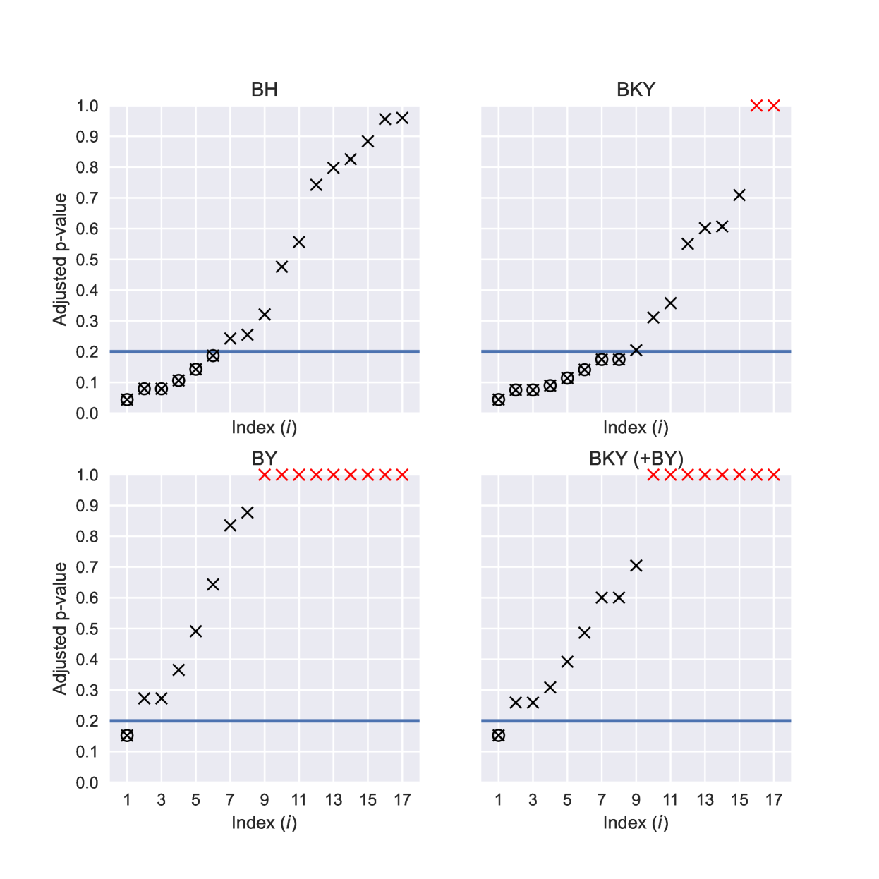
Figure 2: Comparison of fdr-adjusted p-values produced with different methods, for the same data shown in Figure 1. Each symbol $\boldsymbol{\times}$ represents a uncorrected p-value; these are placed in ascending order ($i$); the p-values considered significant are surrounded by a circle $\boldsymbol{\otimes}$. The adjustment ensures that a single, fixed threshold can be applied to all tests (blue line; $q=0.20$); values below that threshold are considered significant. Note that adjusted p-values can sometimes be greater than 1; these can be replaced by 1 (markers $\boldsymbol{\times}$ in red).

With adjusted p-values, significance thresholds no longer depend on the position $i$ for bky: maps of adjusted p-values can be arbitrarily thresholded at any $q$ in the interval between 0 and 1 (Figure 2). Using Equation 6 for bky, as opposed to a formulation equivalent to Equation 5, solves the issue with the paradoxical results observed by Reiss et al. (2012), whereby adjusted p-values would seem smaller than their unadjusted counterparts.

For Šidák, Bonferroni, and permutation methods, fwer-corrected p-values are monotonically related to their underlying p-values, such that no distinction between correction or adjustment needs to be made. Šidák-adjusted p-values can be computed as $\left[p_{i}^{\text{\v{S}id\'{a}k}}\right]_{\text{adj}}=1-(1-p_{i})^{V}$, whereas Bonferroni-adjusted p-values can be computed as $\left[p_{i}^{\text{Bonf.}}\right]_{\text{adj}}=p_{i}V$. For permutation methods, adjusted p-values are computed by referring to the distribution of the maximum statistic across tests (Westfall and Young, 1993).

Note that adjusted p-values computed for various fdr procedures or for Bonferroni can be greater than 1; this can be treated by replacing adjusted p-values greater than 1 by 1 (i.e., by Winsorization of adjusted p-values at 1; in Figure 2 these Winsorized, adjusted p-values are marked in red).

2.5 Strong and weak control

Methods for controlling fwer and fdr differ not only on the measurement of error that is controlled, but on at least another aspect: the methods used for fwer in imaging provide strong control over the error rate, whereas those for fdr provide weak control. Strong control means that the error rate is controlled for any configuration of true and false null hypotheses; in contrast, weak control pertains to controlling the error rate under certain conditions, such as the complete null (Hochberg and Tamhane, 1987; Nichols and Hayasaka, 2003; Proschan and Brittain, 2020). With fdr, weak control ensures that the average proportion of erroneous rejections, given that any rejections occur, is limited to a pre-specified level. While strong control guarantees a bound on errors irrespective of the underlying truth, weak control emphasizes average performance, which can be more lenient but also adaptive to the amount of effects present in the data. In the case of fdr, this has important yet little appreciated consequences on how statistical maps are visualized and interpreted, particularly when using two-tailed tests, as discussed below.

2.6 Discrete p-values

Permutation and other resampling-based methods for inference produce p-values that are discrete. In a permutation test, for example, if a number $J$ of permutations is performed, the smallest possible p-value is $1/J$; all other p-values are multiples $1/J$. Further, if multiple tests are performed, a large number of ties (identical p-values) are expected to occur. The fdr-controlling procedures discussed here make use of the rank $(i)$ of p-values. Even though in many rank-based statistical tests, ties are replaced by their average rank (Hollander et al., 2014), this is not necessary with these procedures: tied p-values can be sorted randomly within their rank; if any p-value is rejected, regardless of its rank, all others tied up with it will also be rejected. While ties are not of concern, the discreteness causes these procedures to become conservative; the degree of conservativeness depends on the granularity of p-values: the less resolved p-values, the more conservative the correction becomes. The reason is that is may be impossible for some p-values reach the threshold at position $i$ simply because they cannot be small enough. This problem can be solved by running more permutations if the data and experimental design permits. Addressing the fdr conservativeness when the number of permutations is very small and cannot be increased remains an unsolved problem. Of note, fdr-controlling procedures for cases in which the different tests may have p-values with varying degrees of resolution have been proposed (for a review, see Döhler et al., 2018); these do not typically apply to imaging, since under the null, the resolution of the permutation distribution of p-values is the same for all tests (a notable exception is if inference uses the negative binomial approximation; see Winkler et al., 2016).

2.7 Two-tailed tests

If the distribution of the test statistic is symmetric and continuous, two-tailed p-values can be obtained from one-tailed as $p^{\text{two}}=1-\left|2p^{\text{one}}-1\right|$. More generally, if the distribution is either continuous or discrete, two-tailed p-values can be obtained as $p^{\text{two}}=2\cdot\min\left\{p^{\text{one}},1-p^{\text{one}}+C\right\}$, where $C=0$ for continuous (often parametric) p-values, or $C=1/J$ for discrete, permutation-based (non-parametric) p-values, and $J$ is the number of permutations. If the distribution of the test statistics is asymmetric, two-tailed p-values must be obtained from that distribution, even if one-tailed p-values are available.

In principle, using fdr with two-tailed tests is straightforward: the two-tailed p-values are obtained, then an fdr-controlling procedure is applied. For visualization, a number of options can be considered: for example, a map of uncorrected p-values can be thresholded at the fdr-controlling level, or a map of adjusted p-values can be thresholded at the desired level. Alternatively, if the distribution of the test statistic is known, the threshold p-value can be converted to a threshold statistic (using the cumulative distribution function), which can be applied to the partition statistical map into significant and non-significant regions. A thresholded map (of statistics or of p-values) can be binarized and used as a mask to display or select regions for further analyses. As long as inference remains focused equally on all tests, using fdr on two-tailed p-values has nothing special compared to using one-tailed p-values. In some circumstances, however, two-tailed tests can become problematic, as discussed below.

2.8 Direction and localization errors

As noted above, fdr does not provide strong control over the error rate, which means that the amount of errors in any subset of tests is not guaranteed to be within the desired level. For two-tailed tests, this becomes problematic if the researcher wishes to draw conclusions pertaining to the direction of effects — that is, inferring about each tail separately. Likewise, this becomes problematic if the researcher wishes to draw conclusions about the amount of errors within specific regions after fdr has been applied globally. To illustrate that, consider these two examples:

Example 1: Direction error

An investigation into the association between cortical thickness (measured at every vertex of a surface representation of the brain) and a behavioral measure involves a sample of hundreds of individuals. Acknowledging that effects could be manifest in either direction, and pursuing statistical rigor, the researcher employs two-tailed p-values, with adjustments for multiple testing using an fdr. The map of test statistics is then masked at the significant level $q=0.01$, thus retaining for visualization only the significant vertices. The analysis uncovers large areas in the frontal and parietal lobes with a positive relationship to the behavioral measure, as hypothesized. However, it also reveals a negative association spanning broad portions of the fusiform gyrus, as well as vertices showing positive or negative associations scattered across the cortex. The researcher conducting the analysis writes a report detailing the novel negative findings, emphasizing the stringent methodologies that incorporated two-tailed tests and a strict fdr significance threshold, well below the conventional level $q=0.05$, and concludes (erroneously) that only about 1% of the negative associations are expected to be false positives.

Example 2: Localization error

In a study of a compound for reducing the severity of relapses in multiple sclerosis (ms), white matter hyperintensities (wmh) are analyzed voxelwise. Subjects are randomly allocated into active compound and placebo groups. Based on prior knowledge and on random population sampling, normality is assumed and a two-sided group comparison is conducted using a two-sample $t$-test. This produces two-tailed p-values, calculated from the Student’s $t$-distribution. Control for multiple testing across voxels is achieved using fdr at $q=0.05$. After determining the fdr threshold, the inverse cumulative distribution function of the Student’s $t$-distribution is used to derive the critical threshold $t_{\textsc{fdr}}$. Given the two-tailed nature of the test, symmetrical thresholds $+t_{\textsc{fdr}}$ and $-t_{\textsc{fdr}}$ are set in an image visualization tool. The results show a notable reduction in the periventricular wmh load in the group that used the active compound, as expected (and hoped), as well as mixed results in various juxtacortical regions, albeit with mostly increases in wmh load in these areas. In the report, the investigator concludes (erroneously) that the drug may amplify the wmh load in juxtacortical areas given that, as fdr was used, no more than 5% of the observed changes are false positives.

At first, it may seem that the researchers in both examples did everything correctly, going as far as using two-tailed tests and ensuring that the multiplicity of tests would be addressed rigorously. A casual reader of the respective study reports may find no issue. Yet, where it comes to statements about the direction or localization of effects, the interpretation is not that, among the findings in the negative direction (Example 1) or in a particular region (Example 2), the proportion of false positives is within $q$, but only that the proportion of false positives among all tests that were subjected to fdr is within $q$. The actual, realized (but unknown) fdr is not guaranteed to be within 1% for the negative (or positive) direction in Example 1, nor or 5% within the juxtacortical white matter (or any other region) in Example 2, and can in both cases be anywhere between 0 and 100% in the reported direction or region.

These issues are not inherent to fdr, although they are a consequence of how fdr operates on data and its properties; the cause of the problem is the attempt to make inferences on subsets of the data over which fdr was applied. Localization errors can be avoided by refraining from making statements or from taking actions that could refer to the amount of errors in specific regions when fdr is controlled only globally, or by doing separate fdr analyses within each subset (Efron, 2008). The same holds to avoid direction errors. Direction errors can also be avoided by partitioning the statistical map into two disjoint sets: one with the positive test statistics, another with the negative test statistics, then proceeding to fdr correction in each subset using their two-tailed p-values. This is expected to work because under the null hypothesis, the partitioning using the sign of the test statistic is independent of the two-tailed p-values; the latter are distributed uniformly between 0 and 1 and, in either side of the map, more extreme test statistics (stronger effects) imply lower p-values. Thus, the requirements for fdr, using either bh or bky, are satisfied. The fdr can then be controlled at the desired level $q$ for the positive and for the negative sides of the map. We verify this novel proposition in the next section, along with other methods.

3 Evaluation

3.1 Synthetic data

To assess the realized (empirical) fdr across procedures we used synthetic data formed by 2000 tests, which could represent voxels in a group-level result image. For each, a test statistic $z$ was simulated following a normal distribution with zero mean and unit variance. Five different scenarios were considered for independent test statistics: (i) complete null, with no synthetic effects added; (ii) positive effects only, in which 25% of the tests had their $z$ statistic increased by 3; (iii) negative effects only, in which 25% of the tests had their $z$ statistic decreased by 3; (iv) both positive and negative effects, balanced, in which 25% of the tests had their $z$ statistic increased by 3, another 25% had their $z$ statistic decreased by 3; and (v) both positive and negative effects, unbalanced, in which 10% of the tests had their $z$ statistic increased by 3, another 40% had their $z$ statistic decreased by 3. Another five scenarios (vi–x) were considered; these were identical to the first five except that instead of independent tests, the 2000 test statistics were made non-independent, with a correlation of 0.25. In each scenario, p-values were computed by referring to the normal cumulative distribution function. A summary of the scenarios is shown in Table 1.

Table 1: Scenarios used to evaluate the different fdr approaches with synthetic data. In each scenario, 2000 test statistics were simulated and subjected to fdr procedures. The process was repeated 2000 times.

Simulation scenario	Tests with positive effects	Tests with negative effects	Correlation among tests
i	0%	0%	0
ii	25%	0%	0
iii	0%	25%	0
iv	25%	25%	0
v	10%	40%	0
vi	0%	0%	0.25
vii	25%	0%	0.25
viii	0%	25%	0.25
ix	25%	25%	0.25
x	10%	40%	0.25

Simulations for these 10 scenarios were repeated 2000 times. Each was assessed with both bh and bky. For this simulated data evaluation, we use $q=0.05$. Four different strategies were considered:

• Canonical, in which adjustment is applied to one-tailed p-values in one direction, and to one-tailed p-values in the opposite direction, that is, applied separately to $p$ and to $1-p$. This procedure produces two maps of adjusted p-values, one for each direction; alternatively, it produces two thresholds, one for each direction.

• Combined, in which adjustment is applied simultaneously to one-tailed p-values in the two directions, i.e., on the set formed by $p$ and $1-p$. This procedure produces two maps of adjusted p-values, one for each direction; alternatively, it produces one threshold, to be applied to both directions.

• Two-tailed, in which two-tailed p-values are subjected to adjustment. This procedure produces one map of adjusted p-values; alternatively, it produces one threshold.

• Split-tails, in which the tests are separated into two disjoint subsets, one with positive ($z>0$) and another with negative ($z<0$) statistics; then the two-tailed p-values within each subset are subjected to adjustment. For the cases in which the test statistic is zero ($z=0$), the uncorrected two-tailed p-value is 1, and so is the adjusted p-value. This procedure produces one map of adjusted p-values; alternatively, it produces two thresholds, one for positive test statistics, one for negative test statistics.

For each of the ten scenarios, and for each of the four adjustment methods, which were run with each of bh and bky (80 total sets), the empirical (observed) fdr was calculated. Confidence intervals (95%) were calculated with the Wald method.

3.2 Real data

To assess these four different strategies for two-tailed fdr with real data, as well as to provide an empirical comparison between bh and bky, we use a statistical map originally produced as part of the Neuroimaging Analysis Replication and Prediction Study (narps — Botvinik-Nezer et al., 2020). The narps was an effort to assess the variability of results among different analysis teams analyzing the same imaging dataset. In the study, the teams were provided with the same raw functional magnetic resonance imaging (fmri) data, collected during a gambling task. Each team analyzed the data to investigate predefined hypotheses about brain activation related to gains and losses, and employed diverse analysis workflows, with no two teams choosing identical pipelines. We use (for no particular reason) the maps produced by team 9U7M for narps hypothesis 1. Note that the specifics of the hypothesis are not relevant for the present analysis; consult Botvinik-Nezer et al. (2020) for details about data acquisition, the predefined hypotheses, and the overall narps methodology and its data provenance. For this real data evaluation, we use $q=0.05$.

4 Results

4.1 Synthetic data

Table 2 summarizes the results for the analyses using synthetic data across the 10 different scenarios that involved varying proportions of true positive and negative effects, as well as dependencies among tests. For a given test, the ideal result is that the confidence interval includes the chosen $q=0.05$ value (represented in percentage, i.e., 5%).

Table 2: Comparison of the false discovery proportions (%) among different fdr methods and correction strategies, when false positives are counted considering one side (positive or negative) or both sides of the statistical map. These results are based on synthetic data. The expected proportion of false discoveries is $q\cdot 100\%=5\%$. Confidence intervals (95%) are shown between parentheses.

	Benjamini–Hochberg				Benjamini–Krieger–Yekutieli
Scenario	Canonical	Combined	Two-tailed	Split-tails	Canonical	Combined	Two-tailed	Split-tails
Both sides:
i	10.2 (8.9–11.6)	5.6 (4.6–6.6)	5.6 (4.6–6.6)	10.1 (8.7–11.4)	10.2 (8.9–11.5)	5.5 (4.5–6.6)	5.5 (4.5–6.6)	10.2 (8.9–11.6)
ii	3.8 (3.7–3.8)	3.8 (3.7–3.8)	3.8 (3.7–3.8)	3.0 (3.0–3.1)	4.7 (4.6–4.7)	4.1 (4.0–4.1)	4.5 (4.4–4.5)	4.3 (4.3–4.4)
iii	4.0 (3.9–4.0)	3.9 (3.9–4.0)	3.9 (3.9–4.0)	3.2 (3.2–3.3)	4.8 (4.8–4.9)	4.2 (4.2–4.3)	4.7 (4.6–4.7)	4.5 (4.5–4.6)
iv	2.6 (2.6–2.6)	2.6 (2.6–2.6)	2.6 (2.6–2.6)	2.6 (2.6–2.6)	3.2 (3.2–3.2)	3.2 (3.2–3.2)	4.3 (4.3–4.3)	4.3 (4.3–4.3)
v	2.6 (2.6–2.6)	2.6 (2.6–2.6)	2.6 (2.6–2.6)	2.3 (2.3–2.4)	3.7 (3.7–3.7)	3.2 (3.1–3.2)	4.3 (4.3–4.3)	4.2 (4.2–4.3)
vi	7.8 (6.7–9.0)	4.5 (3.5–5.4)	4.5 (3.5–5.4)	5.3 (4.4–6.3)	7.1 (6.0–8.2)	3.9 (3.0–4.7)	3.9 (3.0–4.7)	4.9 (3.9–5.8)
vii	4.3 (3.9–4.7)	4.1 (3.7–4.4)	4.1 (3.7–4.4)	2.7 (2.5–3.0)	5.6 (5.1–6.0)	4.3 (4.0–4.6)	4.7 (4.4–5.0)	3.7 (3.4–4.0)
viii	4.3 (4.0–4.7)	3.9 (3.7–4.2)	3.9 (3.7–4.2)	2.8 (2.6–3.1)	5.7 (5.2–6.1)	4.3 (4.0–4.6)	4.7 (4.4–5.1)	3.8 (3.5–4.1)
ix	3.7 (3.5–3.9)	2.7 (2.5–2.8)	2.7 (2.5–2.8)	2.9 (2.7–3.1)	4.7 (4.4–4.9)	3.2 (3.0–3.3)	4.3 (4.1–4.4)	4.5 (4.3–4.7)
x	3.4 (3.2–3.6)	2.6 (2.5–2.7)	2.6 (2.5–2.7)	2.5 (2.4–2.7)	5.0 (4.7–5.3)	3.3 (3.1–3.4)	4.3 (4.1–4.5)	4.4 (4.2–4.6)
Positive side:
i	5.1 (4.1–6.0)	2.8 (2.0–3.5)	2.8 (2.0–3.5)	5.0 (4.0–5.9)	5.2 (4.2–6.2)	3.0 (2.3–3.7)	3.0 (2.3–3.7)	5.2 (4.2–6.2)
ii	3.8 (3.7–3.8)	1.9 (1.9–2.0)	1.9 (1.9–2.0)	3.0 (3.0–3.1)	4.7 (4.6–4.7)	2.1 (2.0–2.1)	2.3 (2.3–2.3)	4.3 (4.3–4.4)
iii	3.8 (3.0–4.6)	99.9 (99.7–100.0)	99.9 (99.7–100.0)	5.2 (4.2–6.2)	4.3 (3.5–5.2)	99.8 (99.5–100.0)	99.9 (99.8–100.0)	5.5 (4.5–6.4)
iv	2.5 (2.5–2.5)	2.5 (2.5–2.5)	2.5 (2.5–2.5)	2.5 (2.5–2.5)	3.1 (3.0–3.1)	3.1 (3.0–3.1)	4.2 (4.2–4.2)	4.2 (4.2–4.2)
v	2.5 (2.4–2.6)	6.0 (5.9–6.0)	6.0 (5.9–6.0)	3.6 (3.5–3.6)	2.6 (2.6–2.7)	7.3 (7.2–7.4)	9.8 (9.7–9.9)	4.4 (4.4–4.5)
vi	4.0 (3.2–4.9)	2.2 (1.6–2.9)	2.2 (1.6–2.9)	2.8 (2.0–3.5)	3.9 (3.1–4.7)	1.9 (1.3–2.6)	1.9 (1.3–2.6)	2.7 (2.0–3.4)
vii	3.6 (3.3–3.9)	1.8 (1.6–2.0)	1.8 (1.6–2.0)	2.3 (2.1–2.5)	5.1 (4.7–5.5)	2.2 (2.0–2.4)	2.5 (2.3–2.7)	3.5 (3.3–3.8)
viii	3.0 (2.3–3.7)	70.1 (68.1–72.1)	70.1 (68.1–72.1)	2.5 (1.8–3.1)	3.4 (2.6–4.2)	73.4 (71.4–75.3)	77.2 (75.4–79.0)	2.9 (2.2–3.7)
ix	2.5 (2.3–2.7)	2.0 (1.8–2.1)	2.0 (1.8–2.1)	2.1 (1.9–2.2)	3.0 (2.8–3.2)	2.3 (2.2–2.5)	3.2 (3.0–3.4)	3.3 (3.1–3.5)
x	2.3 (2.1–2.6)	3.7 (3.5–3.9)	3.7 (3.5–3.9)	2.5 (2.3–2.7)	2.9 (2.6–3.2)	4.9 (4.6–5.1)	6.5 (6.2–6.8)	3.6 (3.3–3.8)
Negative side:
i	5.4 (4.4–6.4)	3.0 (2.3–3.8)	3.0 (2.3–3.8)	5.3 (4.3–6.3)	5.2 (4.3–6.2)	2.8 (2.1–3.5)	2.8 (2.1–3.5)	5.3 (4.3–6.3)
ii	2.8 (2.1–3.5)	99.8 (99.6–100.0)	99.8 (99.6–100.0)	4.0 (3.1–4.9)	3.1 (2.4–3.9)	100.0 (100.0–100.0)	100.0 (100.0–100.0)	4.3 (3.5–5.2)
iii	3.9 (3.9–4.0)	2.1 (2.1–2.1)	2.1 (2.1–2.1)	3.2 (3.2–3.2)	4.8 (4.8–4.9)	2.3 (2.2–2.3)	2.5 (2.5–2.5)	4.5 (4.5–4.6)
iv	2.7 (2.7–2.7)	2.7 (2.7–2.7)	2.7 (2.7–2.7)	2.7 (2.7–2.7)	3.3 (3.3–3.3)	3.3 (3.3–3.3)	4.4 (4.4–4.5)	4.4 (4.4–4.5)
v	2.6 (2.6–2.7)	1.7 (1.7–1.7)	1.7 (1.7–1.7)	2.1 (2.0–2.1)	3.9 (3.9–3.9)	2.1 (2.0–2.1)	2.8 (2.8–2.8)	4.2 (4.2–4.2)
vi	3.9 (3.0–4.7)	2.2 (1.6–2.9)	2.2 (1.6–2.9)	2.6 (1.9–3.4)	3.2 (2.4–4.0)	1.9 (1.3–2.5)	1.9 (1.3–2.5)	2.1 (1.5–2.8)
vii	3.5 (2.7–4.3)	69.3 (67.3–71.3)	69.3 (67.3–71.3)	3.0 (2.3–3.8)	3.1 (2.3–3.9)	72.7 (70.7–74.7)	76.6 (74.7–78.5)	2.9 (2.2–3.6)
viii	3.9 (3.6–4.2)	2.1 (1.9–2.3)	2.1 (1.9–2.3)	2.6 (2.4–2.8)	4.9 (4.6–5.3)	2.2 (2.0–2.3)	2.5 (2.3–2.7)	3.5 (3.3–3.7)
ix	2.7 (2.5–2.8)	2.2 (2.0–2.3)	2.2 (2.0–2.3)	2.2 (2.1–2.4)	3.5 (3.3–3.8)	2.7 (2.6–2.9)	3.7 (3.5–3.9)	3.8 (3.6–4.0)
x	2.6 (2.4–2.7)	1.5 (1.4–1.6)	1.5 (1.4–1.6)	1.8 (1.6–1.9)	4.0 (3.8–4.3)	1.8 (1.7–2.0)	2.6 (2.4–2.8)	3.5 (3.3–3.7)

4.1.1 Correction strategies

In the absence of signal, that is, under the complete null hypothesis, and with independent test statistics, the canonical method worked well when false positives were counted among observed positive test statistics only, or among observed negative test statistics only. In these cases, the empirical false discovery proportion was within the confidence intervals, being neither conservative nor anti-conservative. When false positives were counted among all test statistics (both sides, positive and negative), the observed error rate was twice as large as for each side separately, and thus, twice as large as the nominal test level. Similar behavior was observed for the split-tails method. Combined and two-tailed methods controlled the error rate at the nominal level, albeit became conservative when only one or the other direction was considered.

With only positive or only negative true signal, all four correction strategies produced error rates that were within the expected level for test statistics with the same sign as the signal, even if leaning heavily towards conservativeness. However, for test statistics with the opposite sign as the signal, the observed proportion of false discoveries was not controlled by a large margin, approaching 100% error rate. When both sides were considered to count false positives (that is, all tests considered), the error rate was controlled within the nominal level, leaning again towards conservativeness, albeit less heavily.

With both positive and negative true signal in a balanced scenario, the error rate was controlled regardless of how the error rate was counted (positive test statistics only, negative only, or both). That control, however, leaned towards conservativeness. With unbalanced amounts of signal, which more typically represents real experiments, the error rate was not controlled in the side opposite to the one with a preponderance of true signal, with the nominal error rate lying outside the confidence interval.

4.1.2 fdr methods

While the same patterns above were observed for both bh and bky methods, bky had the advantage of leading to observed false discovery rates that were closer to the nominal level in the presence of signal with the same direction as the observed test statistic, as opposed to leaning towards conservatism as bh. In other words, whenever there was signal, bky was more powerful than bh. However, this also meant that the problems with excess false discoveries observed in the side opposite from where there was more signal was also exacerbated.

4.1.3 Dependencies among tests

The same patterns above were observed for dependent tests. Introduced dependencies did not substantially alter the results when comparing the correction strategies or the different fdr methods.

4.2 Real data

Figure 3 shows maps thresholded at positive and negative sides using the different fdr methods and correction strategies, as well as with uncorrected p-values; the thresholds in each case are also shown.

Figure 3: Thresholded statistical maps using different fdr methods and correction strategies for directional inference, as well as uncorrected, for the narps data. Canonical and split-tails strategies produce generally similar results; likewise, combined and two-tailed methods produce broadly similar maps. Inferences using combined or two-tailed maps should not make directional statements about the results; these are only possible in the canonical and split-tails methods. The figure also shows slight but consistent gains in power with the bky procedure when compared to the usual bh procedure. Only visualization software that allow asymmetrical thresholds can be used to display fdr-corrected results that enable directional inferences.

The uncorrected map is thresholded, at the positive side, at $t_{\text{pos}}=1-t_{\text{cdf}}^{-1}(\alpha/2,\nu)=+1.982$, where $t_{\text{cdf}}^{-1}$ is the inverse cumulative distribution function of the Student’s $t$-distribution, $\nu=107$ are the degrees of freedom for this analysis, and $\alpha=0.05$ is the test level; it is thresholded similarly at the negative side at $t_{\text{neg}}=t_{\text{cdf}}^{-1}(\alpha/2,\nu)=-1.982$. The uncorrected thresholded maps suggests the presence of signal in both positive and negative directions, with a preponderance of effects in the negative side, involving more brain regions, particularly around the cortex.

Similar computations were done for each of the correction methods in Figure 3, which shows the thresholds. The canonical strategy produced no significant results in the positive side of the map; the same for the split-tails strategy. The combined strategy resulted in tests considered significant with both positive and negative test statistics. Since all p-values (for tests investigating positive and negative effects) are pooled in the correction, the thresholds are symmetrical. Here, fewer and smaller regions are identified as significant on the negative side (where there is a preponderance of signal) and some results on the positive side that were not seen with the canonical strategy appear significant. The two-tailed strategy produced broadly similar results as with the combined method. Finally, the split-tails strategy produced results that were visually generally similar as the canonical fdr. While the differences were minute in relation to bh, bky consistently produced slightly lower thresholds, leading to a slight increase in power.

5 Discussion

5.1 Two-tailed tests

Two-tailed tests trace their roots to the first decades of statistics as a scientific discipline. Fisher (1925, p. 47) noted that “in some cases we wish to know the probability that the deviation, known to be positive, shall exceed an observed value, whereas in other cases the probability required is that a deviation, which is equally frequently positive and negative, shall exceed an observed value”. This allows assessment of extreme outcomes in any direction, not restricting hypotheses to a specific one. Similarly, in brain imaging, there are cases in which interest lies on only one of the tails, whereas in others, the interest lies on both tails of the distribution of test statistics. Consider, for example, an fmri study where the same information is presented via visual or auditory cues: some brain areas may be selectively modulated by vision and others by hearing; interesting comparisons involve both directions, i.e., higher involvement of some regions during visual than auditory, and vice-versa. Alternatively, consider a voxel-based morphometry study that compares gray matter volume between professional singers and professional pianists: again one might expect brain regions show differences in one group while other regions show the reverse pattern.

In effect, using two-tailed tests as default has at times been recommended for neuroimaging studies: Chen et al. (2019) argued that “it is difficult to imagine a scenario where this researcher would test all voxels simultaneously for just one directional change”. However, the researcher must be aware that the amount of errors is not guaranteed within a given direction if fdr is applied across all tests. Merely applying fdr methods as integrated into neuroimaging packages such as afni, fsl, FreeSurfer, or spm — each referenced in more than 1000 peer-reviewed publications annually (Poldrack et al., 2019) — then proceeding to directional inferences, does not control the error rate, as illustrated by the synthetic and real data.

5.2 Control of the error rate

The analyses using synthetic data indicate that, while fdr-based adjustment (with either bh or bky) controls the error rate in the set of tests to which the procedure is applied, should the researcher decide to make inferences about direction of effects, extra care is necessary, otherwise such inferences can be affected by excess error rate, which can well amount to up to 100% of the tests about which inference is made if true signal is present in only one side. Simple strategies such as using a two-tailed test, or combining the two sets of results with the directional hypotheses into one single fdr correction, do not guarantee control over the error rate for either direction, even though these control the error rate globally, i.e., when all tests are considered. Such global test, however, provides no information on the direction of effects.

Alternative approaches can be considered. For example, running fdr separately for the two set of p-values with each of the directional hypotheses (the canonical strategy), or running fdr separately for the positive and negative test statistics (the split-tails strategy). The analyses demonstrate that these approaches are able to control the error rate in each direction. However, they come with a penalty: should the null hypothesis be true everywhere, the error rate, which should be at the level $q$ under the complete null, is doubled, approaching $2q$.

While the simulations using synthetic data allow quantification of the observed proportion of false discoveries and how it diverges from the nominal, expected rate, real data allows for the visualization of the different patterns that may be observed in typical studies, depending on the fdr method and correction strategy adopted. With real data, the canonical and split-tails lead to broadly similar statistically significant spatial maps; likewise, the combined and two-tailed strategies were broadly similar one to another. Two-tailed tests can be seen as a particular case of multiple testing correction, since they consider both directions of an effect. Hence, it is not surprising that the the two-tailed strategy produces nearly identical results as the combined strategy, which is similar to correction across contrasts (Alberton et al., 2020).

It should be understood, however, that areas of positive signal that appeared as significant with the two-tailed and combined strategies in the narps dataset example may have emerged simply because there is a preponderance of signal in the negative side of the map. This is because procedures that control fdr are adaptive, that is, they start with a stringent control for the smallest p-value, and proceed in steps, each contingent on the findings of the previous one, progressively loosening stringency and continuing as long as each subsequent test continue to be declared significant (Benjamini and Hochberg, 2000; Nichols, 2007). With two-tailed and combined strategies, the large amount of tests with strong signal in one side of the map (negative in our example) allows more opportunities for tests in the opposite side (positive) to be declared significant. The canonical and split-tails strategies break the opportunities for eventual strong or widespread signals present in one side impact the other.

5.3 Localizing power

Even though the above issues are a direct consequence of fdr not providing strong control over the error rate, routine strategies for data analysis and visualization may obscure this property. For example, the use of symmetrical thresholds is common in imaging visualization software, whereby the user loads a statistical map, and applies a threshold $t$; values above $+t$ are shown in a hot color scheme (e.g., red to yellow), while values below $-t$ are shown in a cool color scheme (e.g., blue to cyan); for two-tailed tests, this seems appropriate and rigorous. Yet, the amount of errors in any direction is not controlled with fdr, only the global amount of errors, something not apparent to the user of such tools. Another situation is when drawing conclusions about the amount of errors within a region after controlling globally; it might seem that controlling the error rate for the whole brain is the most rigorous, such that inferences within sub-regions would be conservative, given that a larger number of tests is taken into account. Yet, the amount of errors within any particular region is not controlled, only the global amount of errors. Any attempt to isolate a particular direction or a particular subset of tests will fail to guarantee the same proportion $q$ of false discoveries within that subset. This example also makes it clear that fdr does not provide localizing power; the proportion of errors is guaranteed only globally.

As mentioned in Section 2.8, such localization and direction errors can be avoided by refraining from making localized or directional statements encompassing subsets of the tests, making only such statements when they refer to the whole set of tests that were subjected to the fdr procedure. Direction errors can also be avoided by using strategies such as those that we named canonical or split-tails. These approaches, however, require that the user is able to display the statistical maps in software that enables non-symmetric thresholds to be used. That is, the ideal imaging tool should accommodate separate thresholds for positive and for the negative side of the map, such that these can be set individually after running fdr with one of these strategies. Currently, very few software packages allow the user to easily set asymmetric thresholds for positive and negative sides of the map. Having this feature available across different imaging software would more easily allow for directional investigations with fdr and visualization of results, even using two-tailed tests.

5.4 More power with bky

An important yet little appreciated fact is that the bh procedure — the most commonly adopted — does not control the amount of false discoveries at the exact level $q$ desired by the researcher, but at a lower level $qV_{0}/V$ that is determined by the (unknown) proportion of tests in which the null hypothesis is true among the total number of tests (Section 2.1). Hence, the procedure is, in fact, conservative in relation to the level desired by the researcher. Despite this, it remains more powerful than procedures that control fwer such as Šidák or Bonferroni; typically, unless $V_{0}=V$ (complete null), $\textsc{fwer}=1$ for any fdr-controlling procedure. Whereas bh is adaptive in the sense that the threshold that determines whether a p-value is significant varies according to the sorted p-value position $i$, with fixed slope given by $q/V$, fwer-controlling procedures as Bonferroni use the same constant, horizontal threshold for all p-values. The bky procedure, allows one to eke out more power by being even more adaptive than bh in that the slope itself, rather than fixed, varies according to the sorted p-value position $i$ as $q/(V+1-i(1-q))$. Thus, as far as power considerations are concerned, the bky procedure is preferable over the bh procedure.

This extra power comes with a computational price: bh runs in $\mathcal{O}(V)$ time, whereas bky runs in $\mathcal{O}(V^{2})$ time. This means that, while the time it takes to run fdr grows linearly with the number of tests to be corrected, for bky it grows quadratically. Another point worth mentioning is that bky-adjusted p-values can easily be above 1 (Figure 2. This is not a unique feature of bky: other multiple testing procedures can also lead to adjusted p-values being higher than 1, the simplest being Bonferroni, that leads to adjusted p-values that are equal to the uncorrected p-values multiplied by the number of tests $V$. This fact does not have substantial implications for hypotheses testing, and can be solved via Winsorization at 1.

5.5 Dependencies among tests

While we only considered one case of dependencies among tests, and observed adequate control over the error rate, existing results in the literature (Genovese et al., 2002; Logan and Rowe, 2004; Reiner-Benaim, 2007) demonstrate that, for typical cases, the modification proposed by Benjamini and Yekutieli (2001) for a more robust control over the false discovery proportion (the by procedure) is not necessary, and that even in the presence of negative correlations, bh, being more substantially more powerful, is preferable over by. That extends to bky as well.

6 Conclusion

While fdr procedures provide more power than fwer methods if many tests are expected to be significant and the user is willing to accept some false positives, caution is warranted when making directional inferences after using two-tailed tests. Strategies like running fdr separately on positive and negative test statistics, or on one-tailed p-values partitioned by hypothesis direction, avoid direction errors and control the false discovery proportion in each tail. However, these strategies lose fdr benefits under the complete null, such as controlling the fwer in these cases. Researchers should refrain from making directional inferences about fdr-corrected maps after two-tailed tests particularly when signals are not symmetrically distributed, since weak control means the proportion of false discoveries is only guaranteed globally; for the same reason, localization of effects within subsets is not possible. The bky procedure allows for additional power, albeit it does not eliminate issues with asymmetric signals. Allowing asymmetric thresholds in neuroimaging software would enable appropriate visualization after partitioned fdr.

Source code

Code related to this paper is available at https://github.com/andersonwinkler/fdrfun.

Author contributions

All authors contributed to all aspects of this research.

Competing interests

None.

References

- Alberton et al. (2020) Alberton, B.A., Nichols, T.E., Gamba, H.R., Winkler, A.M., 2020. Multiple testing correction over contrasts for brain imaging. NeuroImage 216, 116760. doi:10.1016/j.neuroimage.2020.116760.
- Benjamini and Hochberg (1995) Benjamini, Y., Hochberg, Y., 1995. Controlling the false discovery rate: a practical and powerful approach to multiple testing. Journal of the Royal Statistical Society. Series B (Methodological) 57, 289–300. doi:10.1111/j.2517-6161.1995.tb02031.x.
- Benjamini and Hochberg (2000) Benjamini, Y., Hochberg, Y., 2000. On the Adaptive Control of the False Discovery Rate in Multiple Testing with Independent Statistics. Journal of Educational and Behavioral Statistics 25, 60–83. doi:10.3102/107699860250010.
- Benjamini et al. (2006) Benjamini, Y., Krieger, A.M., Yekutieli, D., 2006. Adaptive linear step-up procedures that control the false discovery rate. Biometrika 93, 491–507. doi:10.1093/biomet/93.3.491.
- Benjamini and Yekutieli (2001) Benjamini, Y., Yekutieli, D., 2001. The control of the false discovery rate in multiple testing under dependency. The Annals of Statistics 29, 1165–1188. doi:10.1214/aos/1013699998.
- Bonferroni (1936) Bonferroni, C., 1936. Teoria statistica delle classi e calcolo delle probabilità. Pubblicazioni del R. Istituto Superiore di Scienze Economiche e Commericiali di Firenze 8, 3–62.
- Botvinik-Nezer et al. (2020) Botvinik-Nezer, R., Holzmeister, F., Camerer, C.F., Dreber, A., Huber, J., Johannesson, M., Kirchler, M., Iwanir, R., Mumford, J.A., Adcock, R.A., Avesani, P., Baczkowski, B.M., Bajracharya, A., Bakst, L., Ball, S., Barilari, M., Bault, N., Beaton, D., Beitner, J., Benoit, R.G., Berkers, R.M.W.J., Bhanji, J.P., Biswal, B.B., Bobadilla-Suarez, S., Bortolini, T., Bottenhorn, K.L., Bowring, A., Braem, S., Brooks, H.R., Brudner, E.G., Calderon, C.B., Camilleri, J.A., Castrellon, J.J., Cecchetti, L., Cieslik, E.C., Cole, Z.J., Collignon, O., Cox, R.W., Cunningham, W.A., Czoschke, S., Dadi, K., Davis, C.P., Luca, A.D., Delgado, M.R., Demetriou, L., Dennison, J.B., Di, X., Dickie, E.W., Dobryakova, E., Donnat, C.L., Dukart, J., Duncan, N.W., Durnez, J., Eed, A., Eickhoff, S.B., Erhart, A., Fontanesi, L., Fricke, G.M., Fu, S., Galván, A., Gau, R., Genon, S., Glatard, T., Glerean, E., Goeman, J.J., Golowin, S.A.E., González-García, C., Gorgolewski, K.J., Grady, C.L., Green, M.A., Guassi Moreira, J.F., Guest, O., Hakimi, S., Hamilton, J.P., Hancock, R., Handjaras, G., Harry, B.B., Hawco, C., Herholz, P., Herman, G., Heunis, S., Hoffstaedter, F., Hogeveen, J., Holmes, S., Hu, C.P., Huettel, S.A., Hughes, M.E., Iacovella, V., Iordan, A.D., Isager, P.M., Isik, A.I., Jahn, A., Johnson, M.R., Johnstone, T., Joseph, M.J.E., Juliano, A.C., Kable, J.W., Kassinopoulos, M., Koba, C., Kong, X.Z., Koscik, T.R., Kucukboyaci, N.E., Kuhl, B.A., Kupek, S., Laird, A.R., Lamm, C., Langner, R., Lauharatanahirun, N., Lee, H., Lee, S., Leemans, A., Leo, A., Lesage, E., Li, F., Li, M.Y.C., Lim, P.C., Lintz, E.N., Liphardt, S.W., Losecaat Vermeer, A.B., Love, B.C., Mack, M.L., Malpica, N., Marins, T., Maumet, C., McDonald, K., McGuire, J.T., Melero, H., Méndez Leal, A.S., Meyer, B., Meyer, K.N., Mihai, G., Mitsis, G.D., Moll, J., Nielson, D.M., Nilsonne, G., Notter, M.P., Olivetti, E., Onicas, A.I., Papale, P., Patil, K.R., Peelle, J.E., Pérez, A., Pischedda, D., Poline, J.B., Prystauka, Y., Ray, S., Reuter-Lorenz, P.A., Reynolds, R.C., Ricciardi, E., Rieck, J.R., Rodriguez-Thompson, A.M., Romyn, A., Salo, T., Samanez-Larkin, G.R., Sanz-Morales, E., Schlichting, M.L., Schultz, D.H., Shen, Q., Sheridan, M.A., Silvers, J.A., Skagerlund, K., Smith, A., Smith, D.V., Sokol-Hessner, P., Steinkamp, S.R., Tashjian, S.M., Thirion, B., Thorp, J.N., Tinghög, G., Tisdall, L., Tompson, S.H., Toro-Serey, C., Torre Tresols, J.J., Tozzi, L., Truong, V., Turella, L., van ’t Veer, A.E., Verguts, T., Vettel, J.M., Vijayarajah, S., Vo, K., Wall, M.B., Weeda, W.D., Weis, S., White, D.J., Wisniewski, D., Xifra-Porxas, A., Yearling, E.A., Yoon, S., Yuan, R., Yuen, K.S.L., Zhang, L., Zhang, X., Zosky, J.E., Nichols, T.E., Poldrack, R.A., Schonberg, T., 2020. Variability in the analysis of a single neuroimaging dataset by many teams. Nature 582, 84–88. doi:10.1038/s41586-020-2314-9.
- Chen et al. (2019) Chen, G., Cox, R.W., Glen, D.R., Rajendra, J.K., Reynolds, R.C., Taylor, P.A., 2019. A tail of two sides: Artificially doubled false positive rates in neuroimaging due to the sidedness choice with t-tests. Human Brain Mapping 40, 1037–1043. doi:10.1002/hbm.24399.
- Chen et al. (2009) Chen, S., Wang, C., Eberly, L.E., Caffo, B.S., Schwartz, B.S., 2009. Adaptive control of the false discovery rate in voxel-based morphometry. Human Brain Mapping 30, 2304–2311. doi:10.1002/hbm.20669.
- Chumbley and Friston (2009) Chumbley, J.R., Friston, K.J., 2009. False discovery rate revisited: FDR and topological inference using Gaussian random fields. NeuroImage 44, 62–70. doi:10.1016/j.neuroimage.2008.05.021.
- Cox (1996) Cox, R.W., 1996. AFNI: Software for analysis and visualization of functional magnetic resonance neuroimages. Computers and Biomedical Research, an International Journal 29, 162–173. doi:10.1006/cbmr.1996.0014.
- Dunn (1961) Dunn, O.J., 1961. Multiple comparisons among means. Journal of the American Statistical Association 56, 52–64. doi:10.2307/2282330.
- Döhler et al. (2018) Döhler, S., Durand, G., Roquain, E., 2018. New FDR bounds for discrete and heterogeneous tests. Electronic Journal of Statistics 12. doi:10.1214/18-EJS1441.
- Efron (2008) Efron, B., 2008. Simultaneous inference: When should hypothesis testing problems be combined? Annals of Applied Statistics 2, 197–223. doi:10.1214/07-AOAS141.
- Fisher (1925) Fisher, R.A., 1925. Statistical Methods for Research Workers. Oliver & Boyd, Edinburgh.
- Forman et al. (1995) Forman, S.D., Cohen, J.D., Fitzgerald, M., Eddy, W.F., Mintun, M.a., Noll, D.C., 1995. Improved assessment of significant activation in functional magnetic resonance imaging (fMRI): use of a cluster-size threshold. Magnetic Resonance in Medicine 33, 636–47. URL: http://www.ncbi.nlm.nih.gov/pubmed/7596267, doi:10.1002/mrm.1910330508.
- Genovese et al. (2002) Genovese, C.R., Lazar, N.A., Nichols, T., 2002. Thresholding of statistical maps in functional neuroimaging using the false discovery rate. NeuroImage 15, 870–8. doi:10.1006/nimg.2001.1037.
- Heyde and Seneta (2001) Heyde, C.C., Seneta, E. (Eds.), 2001. Statisticians of the centuries. Springer, New York, NY.
- Hochberg and Tamhane (1987) Hochberg, Y., Tamhane, A.C., 1987. Multiple Comparison Procedures. 1st ed., John Wiley & Sons, Inc.
- Hollander et al. (2014) Hollander, M., Wolfe, D.A., Chicken, E., 2014. Nonparametric Statistical Methods. 3 ed., John Wiley and Sons, New York.
- Holmes et al. (1996) Holmes, A.P., Blair, R.C., Watson, J.D., Ford, I., 1996. Nonparametric analysis of statistic images from functional mapping experiments. Journal of Cerebral Blood Flow and Metabolism 16, 7–22. doi:10.1097/00004647-199601000-00002.
- Kimeldorf and Sampson (1989) Kimeldorf, G., Sampson, A.R., 1989. A framework for positive dependence. Annals of the Institute of Statistical Mathematics 41, 31–45. doi:10.1007/BF00049108.
- Korthauer et al. (2019) Korthauer, K., Kimes, P.K., Duvallet, C., Reyes, A., Subramanian, A., Teng, M., Shukla, C., Alm, E.J., Hicks, S.C., 2019. A practical guide to methods controlling false discoveries in computational biology. Genome Biology 20, 118. doi:10.1186/s13059-019-1716-1.
- Logan and Rowe (2004) Logan, B.R., Rowe, D.B., 2004. An evaluation of thresholding techniques in fMRI analysis. NeuroImage 22, 95–108. doi:10.1016/j.neuroimage.2003.12.047.
- Nichols (2007) Nichols, T., 2007. False discovery rate procedures, in: Friston, K., Ashburner, J., Kiebel, S., Nichols, T., Penny, W. (Eds.), Statistical Parametric Mapping. Academic Press, London, pp. 246–252. doi:https://doi.org/10.1016/B978-012372560-8/50020-6.
- Nichols and Hayasaka (2003) Nichols, T., Hayasaka, S., 2003. Controlling the familywise error rate in functional neuroimaging: a comparative review. Statistical methods in medical research 12, 419–46. doi:10.1191/0962280203sm341ra.
- Nichols and Holmes (2002) Nichols, T.E., Holmes, A.P., 2002. Nonparametric permutation tests for functional neuroimaging: a primer with examples. Human Brain Mapping 15, 1–25. doi:10.1002/hbm.1058.
- Poldrack et al. (2019) Poldrack, R.A., Gorgolewski, K.J., Varoquaux, G., 2019. Computational and informatic advances for reproducible data analysis in neuroimaging. Annual Review of Biomedical Data Science 2, 119–138. doi:10.1146/annurev-biodatasci-072018-021237.
- Poline and Mazoyer (1993) Poline, J.B., Mazoyer, B.M., 1993. Analysis of Individual Positron Emission Tomography Activation Maps by Detection of High Signal-to-Noise-Ratio Pixel Clusters. Journal of Cerebral Blood Flow & Metabolism 13, 425–437. doi:10.1038/jcbfm.1993.57.
- Proschan and Brittain (2020) Proschan, M.A., Brittain, E.H., 2020. A primer on strong vs weak control of familywise error rate. Statistics in Medicine 39, 1407–1413. doi:10.1002/sim.8463.
- Reiner-Benaim (2007) Reiner-Benaim, A., 2007. FDR control by the BH procedure for two-sided correlated tests with implications to gene expression data analysis. Biometrical Journal 49, 107–126. doi:10.1002/bimj.200510313.
- Reiss et al. (2012) Reiss, P.T., Schwartzman, A., Lu, F., Huang, L., Proal, E., 2012. Paradoxical results of adaptive false discovery rate procedures in neuroimaging studies. NeuroImage 63, 1833–1840. doi:10.1016/j.neuroimage.2012.07.040.
- Sarkar (1969) Sarkar, T.K., 1969. Some lower bounds of reliability. Technical Report 124. Stanford University.
- Westfall and Young (1993) Westfall, P.H., Young, S.S., 1993. Resampling-Based Multiple Testing: Examples And Methods for p-Value Adjustment. John Wiley and Sons, New York.
- Winkler et al. (2016) Winkler, A.M., Ridgway, G.R., Douaud, G., Nichols, T.E., Smith, S.M., 2016. Faster permutation inference in brain imaging. NeuroImage 141, 502–516. doi:10.1016/j.neuroimage.2016.05.068.
- Winkler et al. (2014) Winkler, A.M., Ridgway, G.R., Webster, M.A., Smith, S.M., Nichols, T.E., 2014. Permutation inference for the general linear model. NeuroImage 92, 381–97. doi:10.1016/j.neuroimage.2014.01.060.
- Worsley et al. (1996) Worsley, K.J., Marrett, S., Neelin, P., Vandal, A.C., Friston, K.J., Evans, A.C., 1996. A unified statistical approach for determining significant signals in images of cerebral activation. Human Brain Mapping 4, 58–73. doi:10.1002/(SICI)1097-0193(1996)4:1<58::AID-HBM4>3.0.CO;2-O.
- Worsley et al. (2004) Worsley, K.J., Taylor, J.E., Tomaiuolo, F., Lerch, J., 2004. Unified univariate and multivariate random field theory. NeuroImage 23 Suppl 1, S189–95. doi:10.1016/j.neuroimage.2004.07.026.
- Yekutieli and Benjamini (1999) Yekutieli, D., Benjamini, Y., 1999. Resampling-based false discovery rate controlling multiple test procedures for correlated test statistics. Journal of Statistical Planning and Inference 82, 171–196. doi:10.1016/S0378-3758(99)00041-5.