Mpemba meets Newton: Exploring the Mpemba and Kovacs effects in the time-delayed cooling law

Abstract

Despite extensive research, the fundamental physical mechanisms underlying the Mpemba effect, a phenomenon where a substance cools faster after initially being heated, remain elusive. Although historically linked with water, the Mpemba effect manifests across diverse systems, sparking heightened interest in Mpemba-like phenomena. Concurrently, the Kovacs effect, a memory phenomenon observed in materials like polymers, involves rapid quenching and subsequent temperature changes, resulting in nonmonotonic relaxation behavior. This paper probes the intricacies of the Mpemba and Kovacs effects within the framework of the time-delayed Newton’s law of cooling, recognized as a simplistic yet effective phenomenological model accommodating memory phenomena. This law allows for a nuanced comprehension of temperature variations, introducing a time delay ($\tau$) and incorporating specific protocols for the thermal bath temperature, contingent on a defined waiting time ($t_{\text{w}}$). Remarkably, the relevant parameter space is two-dimensional ($\tau$ and $t_{\text{w}}$), with bath temperatures exerting no influence on the presence or absence of the Mpemba effect or the relative strength of the Kovacs effect. The findings enhance our understanding of these memory phenomena, providing valuable insights applicable to researchers across diverse fields, ranging from physics to materials science.

I Introduction

As a teenager, Erasto Bartholomeo Mpemba (1950–2023) accidentally discovered the paradoxical effect that now bears his name. In the first part of his renowned paper [1] with Denis Gordon Osborne (1932–2014), the 19-year-old Mpemba candidly recounted the story. In the second part of the paper, Osborne wrote “The headmaster of Mkwawa High School invited me to speak to the students on ‘Physics and national development’. […] One student raised a laugh from his colleagues with a question I remember as ‘If you take two beakers with equal volumes of water, one at $35^{\circ}$C and the other at $100^{\circ}$C, and put them into a refrigerator, the one that started at $100^{\circ}$C freezes first. Why?’. It seemed an unlikely happening, but the student insisted that he was sure of the facts. I confess that I thought he was mistaken but fortunately remembered the need to encourage students to develop questioning and critical attitudes. No question should be ridiculed. In this case there was an added reason for caution, for everyday events are seldom as simple as they seem and it is dangerous to pass a superficial judgment on what can and cannot be. I said that the facts as they were given surprised me because they appeared to contradict the physics I knew. But I added that it was possible that the rate of cooling might be affected by some factor I had not considered. I promised I would put the claim to the test of experiment and encouraged my questioner to repeat the experiment himself.” In that second part of Ref. [1], Osborne reported some experimental results confirming the effect, although he conceded that “The experiments attempted were relatively crude and several factors could influence cooling rates. More sophisticated experiments are needed to provide a more certain answer to the question.”

The above paragraph succinctly states what the Mpemba effect is about—the possibility that hot water freezes faster than cold water. But, more importantly, Osborne emphasizes the importance of fostering a spirit of curiosity and open-mindedness in scientific inquiry. When confronted with a seemingly counterintuitive claim by a student, Osborne resisted the temptation to dismiss or ridicule the idea outright. Instead, he acknowledged the potential limitations of his own understanding and expressed a willingness to explore the claim through experimentation. This approach reflects a commitment to the principle that scientific inquiry should be driven by evidence and an openness to reevaluate established beliefs in the face of new and unexpected observations. Osborne’s response underscores the idea that questioning assumptions and testing unconventional ideas can lead to a deeper understanding of the complexities inherent in scientific phenomena.

After 1969, attention to the Mpemba effect was mainly confined to popular science and education journals [2, 3, 4, 5, 6, 7, 8, 9, 10, 11, 12, 13, 14, 15, 16, 17, 18, 19, 20, 21, 22, 23]. It was also revealed that the phenomenon had already been noted by classical philosophers and scholars, including Aristotle[24], Roger Bacon [25], Francis Bacon [26], and René Descartes [27]. Interestingly, in the same year that Mpemba and Osborne published their paper, Kell independently published a brief note that began with the statement: “It is widely believed, at least in Canada, that hot water will freeze more quickly than cold water.”

A unanimous agreement remains elusive regarding the fundamental physical mechanisms responsible for the Mpemba effect. Various factors, including water evaporation [2, 3, 7, 28], natural convection [4, 29, 23], disparities in the gas composition of water [9, 30, 16], the effects of supercooling, either independently [12, 31, 32] or in combination with other factors [33, 34, 35, 36], lack of energy equipartition [37], or the influence of rough walls in creating nucleation sites [38], have been proposed as potential contributors to the Mpemba effect. Conversely, doubts have been raised about the very existence of the Mpemba effect in water [39, 38, 40].

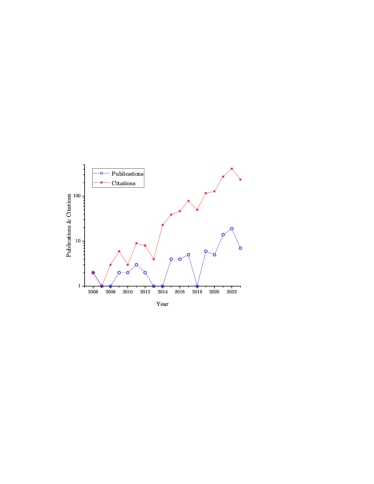
Figure 1: Number of publications and citations in the period 2006–2023 obtained from the Web of Science with the search query “topic=(Mpemba effect).” Note that the data for the year 2023 are not final.

In addition to its historical association with water, the Mpemba effect exhibits similar phenomena reported across a diverse range of systems, including carbon nanotube resonators [41], clathrate hydrates [42], Markovian models [43, 44, 45, 46, 47, 48], granular gases [49, 50, 51, 52, 53, 54, 55, 56, 57, 58], spin glasses [59], molecular gases under drag [60, 61, 62], non-Markovian mean-field systems [63, 64], inertial suspensions [65, 66], colloidal systems [67, 68, 45, 69, 70] quantum systems [71, 72, 73], Ising-like models [74, 75, 76, 48, 77], ideal gases [78], phase transitions [79], active matter [80], the autonomous information engine [81], ionic liquids [82], polymers [83, 84], or Langevin systems [85] The escalating interest in Mpemba-like effects is depicted in Fig. 1.

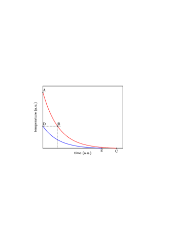
Figure 2: Sketch of supposed cooling curves for two similar systems in same environment. Adapted from Ref. [8].

To elucidate the counterintuitive nature of the Mpemba effect, consider the following excerpt from Osborne [8]:

“Why is the effect unexpected? We suppose the rate of heat transfer to depend on the temperature difference between the cooling system and its environment, and not to depend on its previous history. This is represented in Fig. 2, a sketch of supposed cooling curves showing temperature against time for two similar systems placed in the same environment at the same time but at different initial temperatures. The hot water takes a finite time to cool down to the starting temperature of the cooler water. We expect this system then to be identical to the cooler system when it was first placed in the freezer, that is for the hot starter and the cooler system to be identical at the points represented by B and D on the sketch. Subsequent cooling should also be identical, so that the cooling curve BC should be similar to the cooling curve DE.

But the subsequent cooling is not identical (the overtaking effect would be represented by the curve BC cutting the curve DE). Hence the states of the two systems when represented by the points B and D are not identical. Any explanation for the overtaking effect should enable us to describe the difference between the two systems as represented by the points B and D in such a way that we would expect the system starting hotter to cool faster even below this temperature. What differences might there be?”

Osborne’s depiction in his first “common-sense” paragraph is aptly illustrated by Newton’s law of cooling [86, 87, 88],

$$\dot{T}(t)=-\lambda\left[T(t)-T_{\text{b}}\right],$$ (1)

where $T_{\text{b}}$ is the temperature of the thermal bath (or environment) and $\lambda$ is the coefficient of heat transfer, here assumed to be a (positive) constant. The general solution is simply

$$T(t)=T_{\text{b}}+\left(T_{0}-T_{\text{b}}\right)e^{-\lambda t},$$ (2)

with $T_{0}=T(0)$ being the initial temperature. On the other hand, if the Mpemba effect exists in a certain material, memory dynamics must be taken into account, so that “the overtaking effect should enable us to describe the difference between the two systems as represented by the points B and D [see Fig. 2] in such a way that we would expect the system starting hotter to cool faster even below this temperature.” The simplest way of incorporating those memory phenomena into Newton’s law involves postulating that the temperature’s rate of change at time $t$ depends on the temperature at a preceding time $t-\tau$ [89], i.e.,

$$\dot{T}(t)=-\lambda\left[T(t-\tau)-T_{\text{b}}(t)\right],$$ (3)

where $\tau>0$ is the time delay and we have considered the possibility that the bath temperature, $T_{\text{b}}(t)$, changes with time. Equation (3) can be considered as the simplest phenomenological equation incorporating memory effects.

Additionally to the Mpemba effect, another fascinating memory phenomenon is the Kovacs effect, originally reported in polymer materials [90, 91] and also observed in other complex systems [92, 93, 94, 95, 96, 97, 98, 99, 57]. In the Kovacs effect, a sample, initially in equilibrium at a high temperature $T_{\text{b}}^{-}$, undergoes rapid quenching to a lower temperature $T_{\text{b}}^{+}$. The sample evolves for a specified waiting time $t_{\text{w}}$, but subsequently the bath temperature is abruptly raised to $T(t_{\text{w}})$. Beyond $t=t_{\text{w}}$, the sample temperature exhibits a dynamic behavior: it initially increases, reaches a maximum, and then returns to equilibrium for a longer period. The effect thus highlights the nontrivial impact of the material’s thermal past on its present and future behavior.

The aim of this paper is to analyze the Mpemba and Kovacs effects as described by the time-delayed cooling law, Eq. (3). Its general solution is studied in Sec. II, with special attention to single and double quenches. It is seen that, in the former case, the solution has a form similar to Eq. (2), except that the role of the exponential $e^{-\lambda t}$ is played by a function $\mathcal{E}(t)$, here called the $\tau$-exp function. This function is positive definite only if the time delay is smaller than a threshold value $\tau_{\max}=\lambda^{-1}e^{-1}$. Next, in Sec. III, the solution is applied to the study of the Mpemba effect under simple protocols involving a hot bath at temperature $T_{\text{b}}^{\text{h}}$ and a cold bath at temperature $T_{\text{b}}^{\text{c}}$. Sample A is thermalized at temperature $T_{\text{b}}^{\text{h}}$ and then quenched to temperature $T_{\text{b}}^{\text{c}}$. Conversely, sample B is thermalized at $T_{\text{b}}^{\text{c}}$, quenched to $T_{\text{b}}^{\text{h}}$, and, after a waiting time $t_{\text{w}}$, quenched again to the cold temperature $T_{\text{b}}^{\text{c}}$. For simplicity, the quench of sample A and the first quench of sample B occur at the same time. After this preparation protocol, both samples are in the same environment (bath $T_{\text{b}}^{\text{c}}$) but start with different temperatures. It is proved in Sec. III that (i) the existence or absence of the Mpemba effect is independent of the values of $T_{\text{b}}^{\text{h}}$ and $T_{\text{b}}^{\text{c}}$, (ii) the Mpemba effect exists if and only if the two control parameters ($\tau$ and $t_{\text{w}}$) lie inside a certain narrow region, and (iii) the direct (cooling process) and the inverse (heating process) effects are fully equivalent. Section IV is devoted to the Kovacs effect and the function characterizing the strength of the Kovacs hump is identified. Interestingly, this hump points downward in the cooling process, thus signaling the presence of an anomalous Kovacs effect [94, 99], which becomes relatively stronger as both the time delay $\tau$ and the waiting time $t_{\text{w}}$ increase. Finally, the paper is closed in Sec. V with a summary and conclusion.

II Time-delayed Newton’s cooling law

II.1 General solution in Laplace space

The general solution of Eq. (3) depends not only on the initial temperature $T_{0}$ but it is actually a functional of the previous history $T(t)$ for $-\tau<t<0$. Given the linear character of Eq. (3), it is convenient to define the Laplace transforms

$$\widetilde{T}(s)=\int_{0}^{\infty}dt\,e^{-st}T(t),\quad\widetilde{T}_{\text{b}}(s)=\int_{0}^{\infty}dt\,e^{-st}T_{\text{b}}(t).$$ (4)

Thus, Eq. (3) becomes

$$s\widetilde{T}(s)-T_{0}=\widetilde{T}_{\text{b}}(s)-e^{-s\tau}\widetilde{T}(s)-\widetilde{H}(s),$$ (5)

where

$$\widetilde{H}(s)=\int_{-\tau}^{0}dt\,e^{-s(t+\tau)}T(t),$$ (6)

and, for simplicity, we have taken $\lambda^{-1}=1$ as unit of time. Thus, the general solution in Laplace space is

$$\widetilde{T}(s)=\frac{1}{s+e^{-s\tau}}\left[T_{0}+\widetilde{T}_{\text{b}}(s)-\widetilde{H}(s)\right].$$ (7)

II.2 Basic solution. Single quench

Let us first consider the simple bath temperature history

$$T_{\text{b}}(t)=\begin{cases}T_{\text{b}}^{-},&t<0,\\ T_{\text{b}}^{+},&t>0.\end{cases}$$ (8)

The system is assumed to have equilibrated at $T_{\text{b}}^{-}$ for $t<0$, that is, $T(t<0)=T_{\text{b}}^{-}$. Then, at $t=0$, the system is quenched to the bath temperature $T_{\text{b}}^{+}$, so that $\lim_{t\to\infty}T(t)=T_{\text{b}}^{+}$.

Our aim is to describe the transient stage from $T(t\leq 0)=T_{\text{b}}^{-}$ to $T(\infty)=T_{\text{b}}^{+}$. In Laplace space, this is described by Eq. (7) with $T_{0}=T_{\text{b}}^{-}$, $\widetilde{T}_{\text{b}}(s)=T_{\text{b}}^{+}s^{-1}$, and

$$\widetilde{H}(s)=T_{\text{b}}^{-}s^{-1}\left(1-e^{-s\tau}\right).$$ (9)

Thus, Eq. (7) reduces to

$$\widetilde{T}(s)=T_{\text{b}}^{+}s^{-1}+\left(T_{\text{b}}^{-}-T_{\text{b}}^{+}\right)\widetilde{\mathcal{E}}(s),$$ (10)

where

$$\widetilde{\mathcal{E}}(s)=s^{-1}-\frac{s^{-2}}{1+s^{-1}e^{-s\tau}}.$$ (11)

Note that $\widetilde{\mathcal{E}}(s)$ is independent of both $T_{\text{b}}^{-}$ and $T_{\text{b}}^{+}$. In real time, one has

$$T(t)=\begin{cases}T_{\text{b}}^{-},&t<0,\\ T_{\text{b}}^{+}+\left(T_{\text{b}}^{-}-T_{\text{b}}^{+}\right)\mathcal{E}(t),&t>0,\end{cases}$$ (12)

$\mathcal{E}(t)$ being the inverse Laplace transform of $\widetilde{\mathcal{E}}(s)$. In the limit of no delay ($\tau\to 0$), $\widetilde{\mathcal{E}}(s)\to(1+s)^{-1}$, so that $\mathcal{E}(t)\to e^{-t}$ and Eq. (2) is recovered. Because of that, henceforth the function $\mathcal{E}(t)$ will be referred to as the $\tau$-exp function .

In general, if $\tau>0$, the function $\mathcal{E}(t)$ characterizes the transient of temperature from $T_{\text{b}}^{-}$ to $T_{\text{b}}^{+}$. To obtain $\mathcal{E}(t)$, let us expand $(1+s^{-1}e^{-s\tau})^{-1}=\sum_{n=0}^{\infty}(-s)^{-n}e^{-ns\tau}$ and rewrite Eq. (11) as

$$\widetilde{\mathcal{E}}(s)=s^{-1}-\sum_{n=0}^{\infty}(-s)^{-(n+2)}e^{-ns\tau}.$$ (13)

Therefore,

$$\mathcal{E}(t)= 1+\sum_{n=0}^{\infty}\frac{(n\tau-t)^{n+1}}{(n+1)!}\Theta(t-n\tau)$$

$$= 1+\sum_{n=0}^{\lfloor{t/\tau}\rfloor}\frac{(n\tau-t)^{n+1}}{(n+1)!},\quad t>0,$$ (14)

where $\Theta(\cdot)$ is the Heaviside step function and $\lfloor\cdot\rfloor$ denotes the floor function. More explicitly,

$$\mathcal{E}(t)=\begin{cases}1-t,&0<t<\tau,\\ 1-t+\frac{(\tau-t)^{2}}{2},&\tau<t<2\tau,\\ 1-t+\frac{(\tau-t)^{2}}{2}+\frac{(2\tau-t)^{3}}{3!},&2\tau<t<3\tau,\\ \cdots,&\cdots\end{cases}$$ (15)

Note that

$$\dot{\mathcal{E}}(t)=-\mathcal{E}(t-\tau).$$ (16)

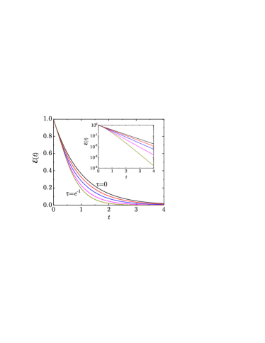
Figure 3: Plot of the $\tau$-exp function $\mathcal{E}(t)$ with, from top to bottom, $\tau=0$, $0.1$, $0.2$, $0.3$, and $e^{-1}\simeq 0.368$. The inset shows the graph in semilogarithmic scale.

Figure 3 shows the $\tau$-exp function $\mathcal{E}(t)$ for several values of $\tau$ in normal (main panel) and semilogarithmic (inset) scales. As we can see, the larger the time delay $\tau$, the faster the decay of $\mathcal{E}(t)$.

The long-time behavior of $\mathcal{E}(t)$ is governed by the dominant pole of $\widetilde{\mathcal{E}}(s)$, that is, the root of the transcendental equation $s+e^{-s\tau}=0$ with the least negative real part. It can be shown that such a root is real ($s=-\kappa$ with $\kappa<\tau^{-1}$) provided that $\tau<\tau_{\max}=e^{-1}\simeq 0.368$ (at which case $\kappa=e\simeq 2.718$). In that domain, $\kappa$ is the real root of $\kappa=e^{\kappa\tau}$, i.e., $\kappa=-\tau^{-1}W_{0}(-\tau)$, where $W_{0}(z)$ is the principal branch of the Lambert function. If, on the other hand, $\tau>\tau_{\max}$, then the dominant root is a pair of complex conjugates, implying an oscillatory behavior with a negative minimum $\mathcal{E}_{\min}=\mathcal{E}(t_{\min})<0$ at a certain time $t=t_{\min}$. The existence of this minimum compromises the positive-definiteness of the solution, Eq. (12). Suppose that $\tau>\tau_{\max}=e^{-1}$ and $T_{\text{b}}^{-}/T_{\text{b}}^{+}>1+|\mathcal{E}_{\min}|^{-1}$. Then, $T(t_{\min})/T_{\text{b}}^{+}=1-(T_{\text{b}}^{-}/T_{\text{b}}^{+}-1)|\mathcal{E}_{\min}|<0$. Therefore, the time-delayed Newton’s cooling law is physically meaningful only if $\tau<\tau_{\max}=e^{-1}$. This is the maximum value of $\tau$ considered in Fig. 3.

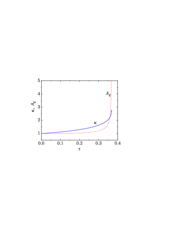
Figure 4: Plot of the damping coefficient $\kappa$ and the amplitude $A_{\mathcal{E}}$ as functions of $\tau$. The circle represents the damping coefficient $\kappa=e\simeq 2.718$ at the maximum time delay $\tau_{\max}=e^{-1}\simeq 0.368$.

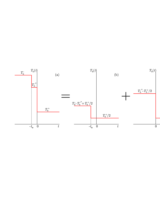
Figure 5: Schematic representation of the decomposition of the double-quench protocol (a) into the sum of the single-quench protocols (b) and (c).

The amplitude $A_{\mathcal{E}}$ of the asymptotic decay of $\mathcal{E}(t)$ is given by the residue of $\widetilde{\mathcal{E}}(s)$ at the pole $s=-\kappa$. Thus,

$$\mathcal{E}(t\gg 1)\approx A_{\mathcal{E}}e^{-\kappa t},\quad A_{\mathcal{E}}=\frac{\kappa^{-1}}{1-\tau\kappa}.$$ (17)

The damping coefficient $\kappa$ and the amplitude $A_{\mathcal{E}}$ are displayed as functions of the time delay $\tau$ in Fig. 4. The damping coefficient increases from $\kappa=1$ at $\tau=0$ to $\kappa=e\simeq 2.718$ at the maximum time delay $\tau_{\max}=e^{-1}\simeq 0.368$. As for the amplitude, it is practically $A_{\mathcal{E}}\simeq 1$ until $\tau\simeq 0.3$, but then it diverges as $\tau$ approaches its maximum value.

Suppose two samples (A and B) subjected to the quench described by Eq. (8), except that the prior bath temperatures are different, say $T_{\text{b,A}}^{-}>T_{\text{b,B}}^{-}$. In that case, according to Eq. (12),

$$T_{\text{A}}(t)-T_{\text{B}}(t)=\begin{cases}T_{\text{b,A}}^{-}-T_{\text{b,B}}^{-},&t<0,\\ (T_{\text{b,A}}^{-}-T_{\text{b,B}}^{-})\mathcal{E}(t),&t>0.\end{cases}$$ (18)

This proves that no Mpemba effect is possible with the one-quench protocol.

II.3 A more complex solution. Double quench

Now, instead of taking the single-quench protocol, Eq. (8), we us assume that the material is kept at a prior temperature $T_{\text{b}}^{-}$ for times $t<-t_{\text{w}}$, next it is quenched to a middle bath temperature $T_{\text{b}}^{-*}$ for $-t_{w}<t<0$, and then (after a waiting time $t_{\text{w}}$) it is quenched again to a final bath temperature $T_{\text{b}}^{+}$. This double-quench protocol is

$$T_{\text{b}}(t)=\begin{cases}T_{\text{b}}^{-},&t<-t_{\text{w}},\\ T_{\text{b}}^{-*},&-t_{\text{w}}<t<0.\\ T_{\text{b}}^{+},&t>0.\end{cases}$$ (19)

A sketch of this protocol is shown in Fig. 5(a). It can be expressed as the sum of the two single-quench protocols represented in Figs. 5(b) and 5(c), respectively. Of course, the decomposition is still valid if an arbitrary constant is added and subtracted to each single-quench protocol, respectively. In general, an $n$fold-quench protocol is equivalent to the sum of $n$ single-quench protocols.

Taking into account the linear character of Eq. (3), the solution associated with the bath protocol given by Eq. (19) can be obtained as the superposition of the solutions associated with the protocols in Figs. 5(b) and 5(c). Therefore,

$$T(t)=T_{1}(t)+T_{2}(t),$$ (20)

where, by application of Eq. (12),

$$T_{1}(t)=\begin{cases}T_{\text{b}}^{-}-T_{\text{b}}^{-*}+T_{\text{b}}^{+}/2,&t<-t_{\text{w}},\\ T_{\text{b}}^{+}/2+(T_{\text{b}}^{-}-T_{\text{b}}^{-*})\mathcal{E}(t+t_{\text{w}}),&t>-t_{\text{w}},\end{cases}$$ (21a)

$$T_{2}(t)=\begin{cases}T_{\text{b}}^{-*}-T_{\text{b}}^{+}/2,&t<0,\\ T_{\text{b}}^{+}/2+(T_{\text{b}}^{-*}-T_{\text{b}}^{+})\mathcal{E}(t),&t>0.\end{cases}$$ (21b)

As a consequence, the solution corresponding to the double quench is

$$T(t)=\begin{cases}T_{\text{b}}^{-},&t<-t_{\text{w}},\\ T_{\text{b}}^{-*}+(T_{\text{b}}^{-}-T_{\text{b}}^{-*})\mathcal{E}(t+t_{\text{w}}),&-t_{\text{w}}<t<0,\\ T_{\text{b}}^{+}+(T_{\text{b}}^{-*}-T_{\text{b}}^{+})\mathcal{E}(t)\\ +(T_{\text{b}}^{-}-T_{\text{b}}^{-*})\mathcal{E}(t+t_{\text{w}}),&t>0.\end{cases}$$ (22)

In particular, at $t=0$,

$$T_{0}=T_{\text{b}}^{-*}+(T_{\text{b}}^{-}-T_{\text{b}}^{-*})\mathcal{E}(t_{\text{w}}).$$ (23)

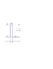
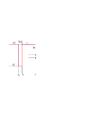
Figure 6: Schematic representation of the protocols A and B for (a) the direct Mpemba effect and (b) the inverse Mpemba effect.

III Mpemba effect

To explore whether the Mpemba effect can be observed from the solutions of the time-delayed Newton’s cooling equation, Eq. (3), we consider two thermal reservoirs, a hot one (at temperature $T_{\text{b}}^{\text{h}}$) and a cold one (at temperature $T_{\text{b}}^{\text{c}}$). Two simple protocols (A and B) are proposed for the Mpemba effect, both direct and inverse, as illustrated in Fig. 6. Let us first describe the protocols for the direct effect, Fig. 6(a). According to protocol A, one sample (A) is first equilibrated at the hot bath temperature $T_{\text{b}}^{\text{h}}$ and then it is suddenly quenched to the cold bath temperature $T_{\text{b}}^{\text{c}}$ at time $t=-t_{\text{w}}$. The other sample (B) is first equilibrated at the cold bath temperature $T_{\text{b}}^{\text{c}}$, then quenched to the hot bath temperature $T_{\text{b}}^{\text{h}}$ at $t=-t_{\text{w}}$, and finally quenched to the cold bath at $t=0$. Thus, sample A experiences a single quench ($T_{\text{b}}^{\text{h}}\to T_{\text{b}}^{\text{c}}$), while sample B is subject to a double quench ($T_{\text{b}}^{\text{c}}\to T_{\text{b}}^{\text{h}}\to T_{\text{b}}^{\text{c}}$). As seen from Fig. 6(b), protocols A and B for the inverse Mpemba effect are the same, except for the exchange $T_{\text{b}}^{\text{h}}\leftrightarrow T_{\text{b}}^{\text{c}}$ (i.e., A: $T_{\text{b}}^{\text{c}}\to T_{\text{b}}^{\text{h}}$; B: $T_{\text{b}}^{\text{h}}\to T_{\text{b}}^{\text{c}}\to T_{\text{b}}^{\text{h}}$).

For the protocols depicted in Fig. 6(a), the temporal evolution of sample A is given by Eq. (22) with $T_{\text{b}}^{-}=T_{\text{b}}^{-*}=T_{\text{b}}^{\text{h}}$ and $T_{\text{b}}^{+}=T_{\text{b}}^{\text{c}}$. Analogously, in the case of sample B, $T_{\text{b}}^{-}=T_{\text{b}}^{+}=T_{\text{b}}^{\text{c}}$ and $T_{\text{b}}^{-*}=T_{\text{b}}^{\text{h}}$. Therefore,

$$T_{\text{A}}(t)=\begin{cases}T_{\text{b}}^{\text{h}},&t<-t_{\text{w}},\\ T_{\text{b}}^{\text{c}}+(T_{\text{b}}^{\text{h}}-T_{\text{b}}^{\text{c}})\mathcal{E}(t+t_{\text{w}}),&t>-t_{\text{w}},\end{cases}$$ (24a)

$$T_{\text{B}}(t)=\begin{cases}T_{\text{b}}^{\text{c}},&t<-t_{\text{w}},\\ T_{\text{b}}^{\text{h}}-(T_{\text{b}}^{\text{h}}-T_{\text{b}}^{\text{c}})\mathcal{E}(t+t_{\text{w}}),&-t_{\text{w}}<t<0,\\ T_{\text{b}}^{\text{c}}+(T_{\text{b}}^{\text{h}}-T_{\text{b}}^{\text{c}})\left[\mathcal{E}(t)-\mathcal{E}(t+t_{\text{w}})\right],&t>0.\end{cases}$$ (24b)

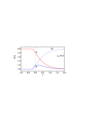
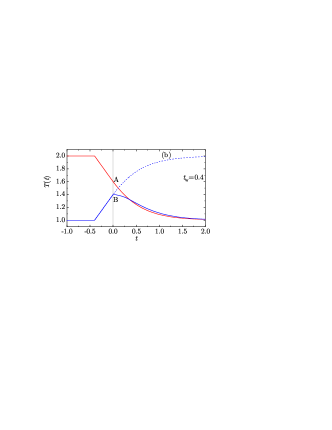
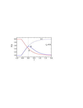
Figure 7: Plot of $T_{\text{A}}(t)$ and $T_{\text{B}}(t)$, including their past history for $t<0$. Here, $T_{\text{b}}^{\text{h}}=2$, $T_{\text{b}}^{\text{c}}=1$, and $\tau=0.36$, with (a) $t_{\text{w}}=0.2$, (b) $t_{\text{w}}=0.4$, and (c) $t_{\text{w}}=0.6$. In each panel, the dashed line represents $T_{\text{B}}(t)$ were not the sample be quenched to $T_{\text{b}}^{\text{c}}$ at $t=0$. Note that a Mpemba effect exists in the case of panel (b) ($t_{\text{w}}=0.4$).

As an example, Fig. 7 shows the time evolution of $T_{\text{A}}(t)$ and $T_{\text{B}}(t)$ for a hot bath at $T_{\text{b}}^{\text{h}}=2$, a cold bath at $T_{\text{b}}^{\text{c}}=1$, a time delay $\tau=0.36$, and three waiting times ($t_{\text{w}}=0.2,0.4,0.6$). As we can see, if the waiting time is too short (for instance, $t_{\text{w}}=0.2$), $T_{\text{B}}(0)$ is so far below $T_{\text{A}}(0)$ that no Mpemba crossing is possible. On the other hand, if the waiting time is too long (for instance, $t_{\text{w}}=0.6$), a crossing takes place during the preparation stage, that is, before sample B is quenched to $T_{\text{b}}^{\text{c}}$ at $t=0$, so that $T_{\text{B}}(0)>T_{\text{A}}(0)$ and again no Mpemba effect occurs. However, if the waiting time is within the right range (for instance, $t_{\text{w}}=0.4$), one has $T_{\text{A}}(0)>T_{\text{B}}(0)$ but sample A cools down sufficiently faster than sample B as to eventually overtake it at a certain crossover time $t_{\times}$ (direct Mpemba effect).

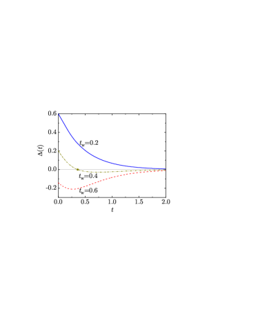
Figure 8: Plot of the difference function $\Delta(t)$ for $\tau=0.36$ and $t_{\text{w}}=0.2$ (—), $0.4$ (–$\cdot$–$\cdot$–), and $0.6$ (– – –). The circle in the curve corresponding to $t_{\text{w}}=0.4$ denotes the corresponding crossover time $t_{\times}$.

Let us now investigate the necessary and sufficient conditions for the existence of the Mpemba effect. From Eqs. (24), we have, for $t\geq 0$,

$$T_{\text{A}}(t)-T_{\text{B}}(t)=(T_{\text{b}}^{\text{h}}-T_{\text{b}}^{\text{c}})\Delta(t),\quad t\geq 0,$$ (25)

where the difference function is

$$\Delta(t)=2\mathcal{E}(t+t_{\text{w}})-\mathcal{E}(t).$$ (26)

For the protocols shown in Fig. 6(b) one would have $T_{\text{A}}(t)-T_{\text{B}}(t)=-(T_{\text{b}}^{\text{h}}-T_{\text{b}}^{\text{c}})\Delta(t)$. Thus, our first observation is that the existence or absence of the Mpemba effect (both direct and inverse) is independent of the bath temperatures $T_{\text{b}}^{\text{h}}$ and $T_{\text{b}}^{\text{c}}$, depending only on the delay time $\tau$ and the waiting time $t_{\text{w}}$ through the difference function $\Delta(t)$. Figure 8 shows the function $\Delta(t)$ for the same values of $\tau$ and $t_{\text{w}}$ as in Fig. 7.

To prevent a situation similar to that illustrated in Fig. 7(c), one must ensure that $\Delta(0)>0$, so that $T_{\text{A}}(0)-T_{\text{B}}(0)>0$ in the direct effect and $T_{\text{A}}(0)-T_{\text{B}}(0)<0$ in the inverse effect. This implies that, for a given delay time $\tau$, the maximum value $t_{\text{w}}^{\max}$ of the waiting time $t_{\text{w}}$ is the solution of $\mathcal{E}(t_{\text{w}})=1/2$. This maximum value ranges from $t_{\text{w}}^{\max}=\ln 2\simeq 0.693$ for $\tau=0$ to $t_{\text{w}}^{\max}\simeq 0.510$ for $\tau=e^{-1}$.

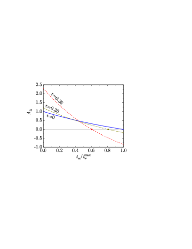
Figure 9: Plot of the amplitude $A_{\Delta}$ as a function of $t_{\text{w}}/t_{\text{w}}^{\max}$ for $\tau=0$ (—), $0.30$ (–$\cdot$–$\cdot$–), and $0.36$ (– – –). The circles in the curves corresponding to $\tau=0.30$ and $0.36$ denote the respective values of $t_{\text{w}}^{\min}/t_{\text{w}}^{\max}$.

Next, once $t_{\text{w}}<t_{\text{w}}^{\max}$ and, therefore, $\Delta(t)>0$, the occurrence of a Mpemba effect requires that $\Delta(t_{\times})=0$ at a certain crossover time $t_{\times}$, so that it asymptotically relaxes to $\Delta(t)\to 0$ from below, as exemplified by the curve with $t_{\text{w}}=0.4$ in Fig. 8. After the crossover time $t_{\times}$, $-\Delta(t)$ presents a maximum at a time $t_{\text{M}}$ given by the solution to $\dot{\Delta}(t)=0$; according to Eqs. (16) and (26), $\dot{\Delta}(t)=-\Delta(t-\tau)$, implying that $t_{\text{M}}=t_{\times}+\tau$.

From Eq. (17), se see that the asymptotic long-time behavior of $\Delta(t)$ is

$$\Delta(t\gg 1)\approx A_{\Delta}e^{-\kappa t},\quad A_{\Delta}=\frac{\kappa^{-1}}{1-\tau\kappa}\left(2e^{-\kappa t_{\text{w}}}-1\right).$$ (27)

The amplitude $A_{\Delta}$ is plotted in Fig. 9 as a function of $t_{\text{w}}/t_{\text{w}}^{\text{max}}$ for $\tau=0$, $0.3$, and $0.36$. Except in the undelayed case ($\tau=0$), we can see that $A_{\Delta}$ becomes negative if $t_{\text{w}}$ is larger than a threshold value $t_{\text{w}}^{\min}$. Therefore, given a time delay $\tau$, the minimum waiting time $t_{\text{w}}^{\min}$ is determined by the condition $A_{\Delta}=0$, that is, $t_{\text{w}}^{\min}=\kappa^{-1}\ln 2$.

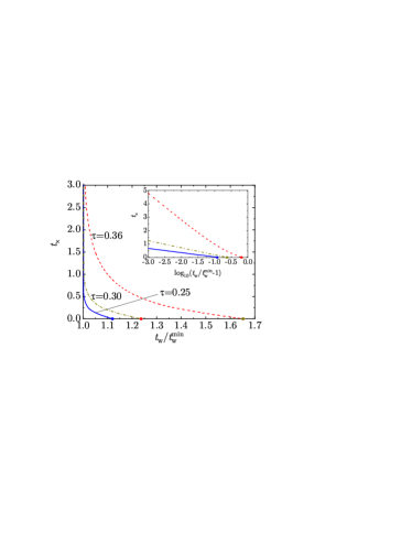
Figure 10: Plot of the crossover time $t_{\times}$ as a function of $t_{\text{w}}/t_{\text{w}}^{\min}$ for $\tau=0.25$ (—), $0.30$ (–$\cdot$–$\cdot$–), and $0.36$ (– – –). The circles denote the respective values of $t_{\text{w}}^{\max}/t_{\text{w}}^{\min}$. The inset shows $t_{\times}$ versus $\log_{10}(t_{\text{w}}/t_{\text{w}}^{\min}-1)$.

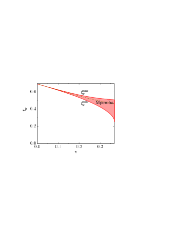
Figure 11: Phase space for the Mpemba effect. The lower and upper curves represent $t_{\text{w}}^{\min}$ and $t_{\text{w}}^{\max}$, respectively, as functions of the delay time $\tau$. If $t_{\text{w}}<t_{\text{w}}^{\min}$, then $\Delta(t)>0$ for $t\geq 0$. If, on the other hand, $t_{\text{w}}>t_{\text{w}}^{\max}$, then $\Delta(t)<0$ for $t\geq 0$. Therefore, the Mpemba effect occurs if and only if $t_{\text{w}}^{\min}<t_{\text{w}}<t_{\text{w}}^{\max}$ (shaded region). The dashed line represents the locus $\Delta(0)=|\Delta(t_{\text{M}})|$.

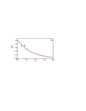
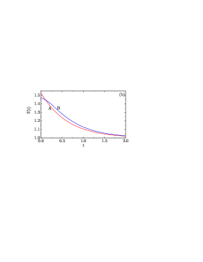
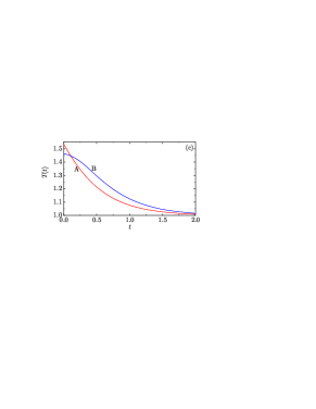
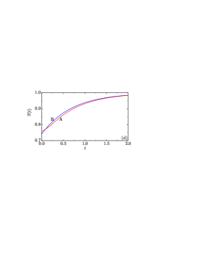
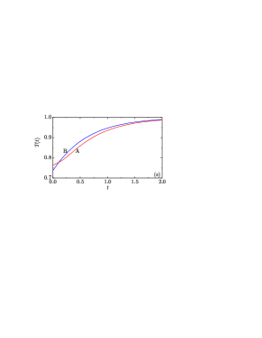
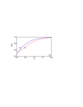
Figure 12: Plot of $T_{\text{A}}(t)$ and $T_{\text{B}}(t)$ for $t>0$. Panels (a, d), (b, e), and (c, f) correspond to $(\tau,t_{\text{w}})=(0.25,0.52)$, $(\tau,t_{\text{w}})=(0.30,0.49)$, and $(\tau,t_{\text{w}})=(0.36,0.47)$, respectively. Panels (a–c) illustrate the direct Mpemba effect (with $T_{\text{b}}^{\text{c}}=1$ and $T_{\text{b}}^{\text{h}}=2$), whereas panels (d–f) illustrate the inverse Mpemba effect (with $T_{\text{b}}^{\text{c}}=0.5$ and $T_{\text{b}}^{\text{h}}=1$).

If $t_{\text{w}}^{\min}<t_{\text{w}}<t_{\text{w}}^{\text{max}}$, the crossover time $t_{\times}$ is characterized by the condition $\Delta(t_{\times})=0$. It is plotted in Fig. 10 as a function of $t_{\text{w}}/t_{\text{w}}^{\min}$ for $\tau=0.25$, $0.3$, and $0.36$. As $t_{\text{w}}$ increases from $t_{\text{w}}^{\min}$ to $t_{\text{w}}^{\max}$, the crossover time $t_{\times}$ decreases monotonically, vanishing at $t_{\text{w}}=t_{\text{w}}^{\max}$. Near $t_{\text{w}}=t_{\text{w}}^{\min}$, $t_{\times}$ diverges logarithmically as $t_{\times}\sim-\ln(t_{\text{w}}/t_{\text{w}}^{\min}-1)$ (see inset of Fig. 10).

In summary, the time-delayed Newton’s cooling equation exhibits a Mpemba effect (either direct or inverse) under the protocols depicted in Fig. 6 if and only if the two only control parameters ($\tau$ and $t_{\text{w}}$) are such that the difference function $\Delta(t)$ fulfills two conditions: (i) $\Delta(0)>0$ (implying $t_{\text{w}}<t_{\text{w}}^{\max}$) and (ii) $\Delta(t)<0$ in the long-time regime (implying $t_{\text{w}}>t_{\text{w}}^{\min}$). The phase space for the occurrence of the Mpemba effect on the plane $t_{\text{w}}$ vs $\tau$ is shown in Fig. 11. Within the shaded Mpemba region, one can say that, for a given time delay $\tau$, the magnitude of the effect is maximal if the waiting time $t_{\text{w}}$ is such that the maximum positive value and the minimum negative value of $\Delta(t)$ are the same (except for the sign), i.e., $\Delta(0)=|\Delta(t_{\text{M}})|$. That line of maximal Mpemba effect is also included in Fig. 11.

Some illustrations of the Mpemba effect (both direct and inverse) are displayed in Fig. 12. The chosen values of $\tau$ and $t_{\text{w}}$ are close to the locus of maximal effect. We observe that, as expected, the Mpemba effect tends to become more pronounced as the time delay $\tau$ increases.

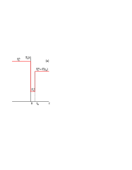
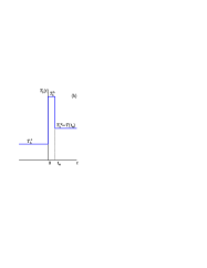
Figure 13: Schematic representation of the protocols for (a) the direct Kovacs effect and (b) the inverse Kovacs effect.

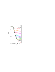
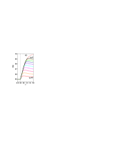
Figure 14: Kovacs effect for $\tau=0.36$ and $t_{\text{w}}=0.1$, $0.2$, …, $1$. Panel (a) corresponds to the direct effect (with $T_{\text{b}}^{\text{h}}=2$ and $T_{\text{b}}^{\text{c}}=1$), whereas panel (b) corresponds to the inverse effect (with $T_{\text{b}}^{\text{c}}=0.5$ and $T_{\text{b}}^{\text{h}}=1$). In each panel, the dashed line represents $T(t)$ were not the sample be quenched to $T(t_{\text{w}})$ at $t=t_{\text{w}}$.

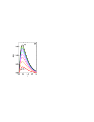
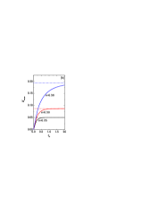
Figure 15: (a) Plot of the Kovacs hump function $K(t)$ for $\tau=0.36$ and $t_{\text{w}}=0.1$, $0.2$, …, $1$. (b) Plot of the maximum value $K_{\max}$ of $K(t)$ as a function of $t_{\text{w}}$ for, from bottom to top, $\tau=0.25$, $0.3$, and $0.36$. The dashed lines represent the asymptotic values $1-\tau-\kappa^{-1}$.

IV Kovacs effect

In the Kovacs effect, the protocol is similar to that of sample B in the Mpemba effect (see Fig. 6), except for a couple of points, as summarized in Fig. 13. First, it is convenient to shift time an amount $t_{\text{w}}$, so that the first quench occurs at $t=0$ and the second one at the waiting time $t=t_{\text{w}}$. Second, the final bath temperature is made to coincide with the instantaneous system’s temperature at $t=t_{\text{w}}$, i.e., $T_{\text{b}}^{+}=T(t_{\text{w}})\equiv T_{\text{b}}^{\text{w}}$. Thus, according to Eq. (22), the temperature in the direct Kovacs effect is

$$T(t)=\begin{cases}T_{\text{b}}^{\text{h}},&t<0,\\ T_{\text{b}}^{\text{c}}+(T_{\text{b}}^{\text{h}}-T_{\text{b}}^{\text{c}})\mathcal{E}(t),&0<t<t_{\text{w}},\\ T_{\text{b}}^{\text{w}}+(T_{\text{b}}^{\text{c}}-T_{\text{b}}^{\text{w}})\mathcal{E}(t-t_{\text{w}})\\ +(T_{\text{b}}^{\text{h}}-T_{\text{b}}^{\text{c}})\mathcal{E}(t),&t>t_{\text{w}},\end{cases}$$ (28)

with

$$T_{\text{b}}^{\text{w}}=T_{\text{b}}^{\text{c}}+(T_{\text{b}}^{\text{h}}-T_{\text{b}}^{\text{c}})\mathcal{E}(t_{\text{w}}).$$ (29)

In the inverse effect, one must set $T_{\text{b}}^{\text{h}}\leftrightarrow T_{\text{b}}^{\text{c}}$.

Figure 14 illustrates the direct and inverse effects for $\tau=0.36$. As can be seen, after the quench at $t=t_{\text{w}}$, the temperature presents a local minimum (maximum) in the direct or cooling (inverse or heating) case. In the direct Kovacs effect, the temperature slope experiences a discontinuity from $\dot{T}(t_{\text{w}}^{-})=-\left[T(t_{\text{w}}-\tau)-T_{\text{b}}^{\text{c}}\right]$ to $\dot{T}(t_{\text{w}}^{+})=-\left[T(t_{\text{w}}-\tau)-T_{\text{b}}^{\text{w}}\right]$ but the sign is negative at both sides of $t=t_{\text{w}}$. Consequently, the Kovacs hump appears below $T=T_{\text{b}}^{\text{w}}$, thus qualifying as an anomalous Kovacs effect [94, 99]. An analogous conclusion holds in the inverse effect, where $\dot{T}(t_{\text{w}}^{-})=T_{\text{b}}^{\text{h}}-T(t_{\text{w}}-\tau)>\dot{T}(t_{\text{w}}^{+})=T_{\text{b}}^{\text{w}}-T(t_{\text{w}}-\tau)>0$ and the hump appears above $T=T_{\text{b}}^{\text{w}}$.

Let us characterize the Kovacs hump in more detail. From Eqs. (28) and (29), one finds that the temperature in the domain $t>t_{\text{w}}$ is

$$T(t)-T_{\text{b}}^{\text{w}}=-(T_{\text{b}}^{\text{w}}-T_{\text{b}}^{\text{c}})K(t-t_{\text{w}}),\quad\text{(direct effect)},$$ (30a)

$$T(t)-T_{\text{b}}^{\text{w}}=(T_{\text{b}}^{\text{h}}-T_{\text{b}}^{\text{w}})K(t-t_{\text{w}}),\quad\text{(inverse effect)},$$ (30b)

where

$$K(t)=\mathcal{E}(t)-\frac{\mathcal{E}(t+t_{\text{w}})}{\mathcal{E}(t_{\text{w}})}$$ (31)

is a semi-definite positive function, henceforth named the Kovacs hump function, which characterizes the relative strength of the Kovacs effect. It vanishes both at $t=0$ and in the limit $t\to\infty$. Note that $\dot{K}(t)=-\mathcal{E}(t-\tau)+\mathcal{E}(t-\tau+t_{\text{w}})/\mathcal{E}(t_{\text{w}})$, so that $\dot{K}(\tau)=0$, implying that $K(t)$ has a maximum value $K_{\max}=1-\tau-\mathcal{E}(\tau+t_{\text{w}})/\mathcal{E}(t_{\text{w}})$ at a time $t_{\text{K}}=\tau$. At a given time delay $\tau$, $K_{\max}$ increases monotonically with increasing waiting time $t_{\text{w}}$, reaching a finite value in the limit $t_{\text{w}}\to\infty$. From Eq. (17), we have $\lim_{t_{\text{w}}\to\infty}K_{\max}=1-\tau-e^{-\kappa\tau}=1-\tau-\kappa^{-1}$.

Figure 15(a) shows the Kovacs hump function $K(t)$ for a time delay $\tau=0.36$ and several values of the waiting time. The maximum value $K_{\max}$ is plotted in Fig. 15(b) as a function of $t_{\text{w}}$ for several values of $\tau$. As expected, the relative strength of the Kovas effect, as measured by $K_{\max}$, increases with increasing $\tau$ y $t_{\text{w}}$.

V Conclusions

Table 1: Summary of the main quantities and results.

Quantity	Symbol	Expression
General
Time delay	$\tau$	Free parameter
Maximum time delay	$\tau_{\max}$	$e^{-1}\simeq 0.368$
$\tau$-exp function	$\mathcal{E}(t)$	$\displaystyle{1+\sum_{n=0}^{\lfloor{t/\tau}\rfloor}\frac{(n\tau-t)^{n+1}}{(n+1)!}}$
Asymptotic decay of $\mathcal{E}(t)$		$\mathcal{E}(t)\approx A_{\mathcal{E}}e^{-\kappa t}$
Damping coefficient	$\kappa$	$\displaystyle{-\tau^{-1}W_{0}(-\tau)}$
Amplitude	$A_{\mathcal{E}}$	$\displaystyle{\frac{\kappa^{-1}}{1-\tau\kappa}}$
Waiting time	$t_{\text{w}}$	Free parameter
Mpemba effect
Difference function	$\Delta(t)$	$2\mathcal{E}(t+t_{\text{w}})-\mathcal{E}(t)$
Minimum waiting time	$t_{\text{w}}^{\min}$	$\kappa^{-1}\ln 2$
Maximum waiting time	$t_{\text{w}}^{\max}$	Root of $\mathcal{E}(t_{\text{w}})=1/2$
Crossover time	$t_{\times}$	Root of $\Delta(t_{\times})=0$
Time when $-\Delta(t)$ is maximum	$t_{\text{M}}$	$t_{\times}+\tau$
Kovacs effect
Kovacs hump function	$K(t)$	$\displaystyle{\mathcal{E}(t)-\frac{\mathcal{E}(t+t_{\text{w}})}{\mathcal{E}(t_{\text{w}})}}$
Time when $K(t)$ is maximum	$t_{\text{K}}$	$\tau$
Maximum value of $K(t)$	$K_{\max}$	$\displaystyle{1-\tau-\frac{\mathcal{E}(\tau+t_{\text{w}})}{\mathcal{E}(t_{\text{w}})}}$

The time-delayed Newton’s cooling law stands out as a seemingly straightforward yet powerful phenomenological model for grasping the intricacies of thermal memory dynamics. This paper has focused on unraveling its solution and applying it to two paradigmatic memory phenomena: the Mpemba and Kovacs effects. The main quantities and results of this work are summarized in Table 1.

A pivotal role is played by the $\tau$-exp function $\mathcal{E}(t)$, functioning as the time-delay analog of the conventional decaying exponential. Imposing the physical condition that $\mathcal{E}(t)>0$ for all time sets an upper bound, $\tau<\tau_{\max}=e^{-1}$, for the time delay.

As the simplest protocol for the observation of the Mpemba effect, we have assumed that samples A and B were thermalized in the past ($t<-t_{\text{w}}$) to the temperatures ($T_{\text{b}}^{\text{h}}$ and $T_{\text{b}}^{\text{c}}$) of a hot and a cold bath, respectively. Sudden quenches at $t=-t_{\text{w}}$ are then applied to both samples by exchanging their baths, followed by a second quench to temperature $T_{\text{b}}^{\text{c}}$ at $t=0$ for sample B. Notably, the time delay enhances the cooling of sample A while inhibiting that of sample B, leading to the Mpemba effect under specific conditions ($t_{\text{w}}^{\min}<t_{\text{w}}<t_{\text{w}}^{\max}$). The effect is independent of the bath temperatures ($T_{\text{b}}^{\text{h}}$ and $T_{\text{b}}^{\text{c}}$) and is determined by a difference function $\Delta(t)$ parameterized by the control parameters $\tau$ and $t_{\text{w}}$. In the inverse Mpemba effect, the protocol is identical, except for the exchange $T_{\text{b}}^{\text{h}}\leftrightarrow T_{\text{b}}^{\text{c}}$, so that the difference function $\Delta(t)$ is the same as in the direct case. Therefore, the time-delayed Newton’s cooling law with a constant coefficient of heat transfer fails to capture the known fact that heating is faster than cooling [100, 101, 70].

The exact solution of the time-delayed cooling equation under a double-quench protocol has also been exploited to study the Kovacs effect. While the system is relaxing from a hot bath temperature ($T_{\text{b}}^{\text{h}}$) to a cold bath temperature ($T_{\text{b}}^{\text{c}}$), it is suddenly put in contact at a waiting time $t_{\text{w}}$ with a bath at temperature $T_{\text{b}}^{\text{w}}=T(t_{\text{w}})$. Instead of maintaining that temperature for $t>t_{\text{w}}$, the memory of a higher temperature in the past ($t<t_{\text{w}}$) makes the system momentarily keep cooling, eventually reaching a minimum temperature at time $t=t_{\text{w}}+\tau$, and finally relaxing to the bath temperature $T_{\text{b}}^{\text{w}}$ from below. This downward hump contrasts with the original one in polymer systems [90, 91] but agrees with the anomalous Kovacs effect observed in granular gases [94, 99]. In analogy with the Mpemba case, a relative strength measure, the Kovacs hump function $K(t)$, remains independent of bath temperatures ($T_{\text{b}}^{\text{h}}$ and $T_{\text{b}}^{\text{c}}$) and increases with $\tau$ and $t_{\text{w}}$.

In conclusion, the time-delayed Newton’s law of cooling emerges as a simplistic yet effective phenomenological model that accommodates memory effects. The exploration of the Mpemba and Kovacs effects within its framework has unveiled significant insights into the intricate nature of these memory phenomena. This paper may contribute to a comprehensive analysis of the Mpemba and Kovacs effects, shedding light on their underlying mechanisms and expanding their relevance to diverse systems. The findings presented here not only deepen our understanding of these memory phenomena but also offer valuable insights applicable across various scientific domains, from physics to materials science. The exploration of time-delayed cooling laws paves the way for future research avenues, inviting further investigation into the fascinating interplay between thermal history, memory effects, and complex system behaviors.

Data availability

The data that support the findings of this study are available from the author on reasonable request.