Vortex dynamics and turbulence in dipolar Bose-Einstein condensates

Abstract

Quantum turbulence indicators in dipolar Bose-Einstein condensed fluids, following emissions of vortex-antivortex pairs generated by a circularly moving detuned laser, are being provided by numerical simulations of the corresponding quasi-two-dimensional Gross-Pitaevskii formalism with repulsive contact interactions combined with tunable dipole-dipole strength. The critical velocities of two variants of a circularly moving obstacle are determined and analyzed for vortex-antivortex nucleation in the form of regular and cluster emissions. The turbulent dynamical behavior is predicted to follow closely the initial emission of vortex-antivortex pairs, relying on the expected Kolmogorov’s classical scaling law, which is verified by the spectral analysis of the incompressible part of the kinetic energy. Within our aim to provide further support in the up-to-now investigations of quantum turbulence, which have been focused on non-dipolar Bose-Einstein condensates, we emphasize the role of dipole-dipole interactions in the fluid dynamics.

I Introduction

Dipole-dipole interactions, which are manifested between particles with permanent electric or magnetic dipoles, have attracted a lot of interest in cold-atom physics. They are expected to lead to novel kinds of degenerate quantum gases even in the weakly interacting limit. The theoretical foundation with related progress can be found in review articles, as in Refs. Baranov2008 ; Lahaye2009 . The control of effective atom-atom dipole interactions under reasonable laboratory conditions was shown to be possible in Ref. 1998Marinescu and following seminal theoretical works reporting the tunability of such interactions 2001Yi ; 2002Santos ; Giovanazzi2002 . Soon after that, it was reported the remarkable observations of dipolar Bose-Einstein condensates (BECs) with isotopes of chromium (⁵²Cr) Griesmaier2006 ; Lahaye2007 ; 2008Koch , dysprosium (¹⁶⁴Dy) Lu2011 ; Youn2010 and erbium (¹⁶⁸Er) Aikawa2012 ; Chomaz2016 . Along with this new exciting branch for investigations opened in cold-atom physics Lahaye2009 ; Baranov2012 ; Fetter2009 ; 2022Klaus ; Chomaz2023 ; 2023Bland , it was recently reported the production of another dipolar BEC with an isotope of europium (¹⁵¹Eu) 2022Miyazawa . Besides their quite different characteristics, the dipole-dipole and contact $s-$wave interactions provide the leading order nonlinear effects, with the dipole-dipole interactions (DDI) being anisotropic with long-range behavior, opposing the short-range contact interactions. In the case of polar atoms, both can be varied widely, from repulsive to attractive, such that they are convenient parameters to control experimental realizations of confined BECs. In order to manipulate $s-$wave contact interactions in cold-atom physics, Feshbach resonance mechanisms have been extensively employed Feshbach1962 , since the first experimental observation of these resonances in a BEC 1998Inouye . When considering polar atoms, we can further control their interactions, either via the magnitude of the external (magnetic or electric) field being applied, or by modulating the alignment of this field with the intrinsic atomic dipole moments, which allows tuning the magnitude and sign of the DDI Giovanazzi2002 ; Kumar2019 . Concerned the stability of dipolar BECs, among the several studies following Ref. 2008Koch , the dynamical stabilization was explored by time modulation of scattering length and using the interplay between nonlinear interactions  Sabari2015 ; Sabari2018a ; Sabari2022 . Noticeable is the crescent interest in binary dipolar mixtures, exploring miscible and immiscible regimes 2012Wilson ; 2017KumarJPC , with an experimental realization (using erbium and dysprosium) reported in 2018Trautman . Along with these studies, the intensive investigations on rotational properties and vortex dynamics with binary dipolar atoms Yi2006 ; Wilson2010 ; Mulkerin2013 ; Zhang2016 ; Kumar2017 ; Sabari2017 ; Martin2017 aim to provide a platform to access plenty of other many-body quantum phenomena, such as the possible creation of long-lived quantum-droplet states and expected connections with superfluidity in BEC.

Quantum vortices in a BEC Fetter2009 can be created only at a minimum critical angular velocity, when energetically favorable, different from their occurrence in normal fluids. Within a realistic experiment, the critical rotation for vortex nucleation can be larger due to dynamical instabilities at the boundaries. In superfluid and superconductor phase transitions, quantum vortices play a prominent role, as known since discoveries related to Helium superfluidity Schwarz1987 and at high-temperature superconductors Blatter1994 . Beyond that, they are commonly observed and investigated in a wide range of contexts going beyond cold-atom physics, such as on exciton-polariton condensates Lagoudakis2008 , on polariton superfluids Sanvitto2010 , and in optics Willner2012 ; Molina2007 . Quantized vortices have been nucleated in BEC through several techniques, such as rotating the trapping potential or thermal cloud 2001Madison (in experiments consistent with following up numerical analysis Tsubota2002 ; Sabari2019 ), stirring the condensate with a blue- or red-detuned laser beam Raman1999 ; Raman2001 ; Neely2010 ; White2012 ; Stagg2015 , moving a condensate past a defect Henn2009 , rapid quench phase transitions of a cooling condensate Lamporesi2013 , or decay instability of a soliton Navon2015 . More recently, vortex nucleations have been applied to lattice configurations 2023Jezek , by predicting vortex positions along low-density paths separating the sites.

Within a recently reported experiment, by applying a moving Gaussian obstacle in a BEC Lim2022 , the authors have shown that a tangle of quantized vortices can be produced. As known from classical fluid dynamics, vortex tangles are understood as a signature of turbulence, with the structure of turbulence being already associated with the flow of incompressible viscous fluids by Kolmogorov Kolmogorov . Since Onsager’s ground-breaking theoretical work linking turbulence with a point vortex dynamics in a two-dimensional (2D) fluid Onsager1949 , it has been hoped that the simple fundamental rules behind quantum theories, together with the recent experimental advances in studying vortex dynamics in superfluids, will aid in understanding the nature of turbulence. As pointed out in 1963 Feynman Lectures on Physics Feynman , the analysis of circulating turbulent fluids is one of the most important problems in nature, left over a hundred years, with nobody really been able to analyze it mathematically satisfactorily still to be solved in spite of its importance. Subsequently, with expectation that some light on the general solution of classical turbulence can be found in the so-called quantum turbulence (QT), the similarities between classical turbulence with superfluidity and QT have been explored in several works and reviews Barenghi2001 ; 2002Vinen ; 2013Skrbek ; 2014Mantia , which are mainly concerned on the classical length scales large, as compared with the characteristic quantum length scale found by the spacing between vortex lines.

After many years of research with superfluid helium systems, QT became a well-established field for investigation, motivating numerous new insights and developments regarding its possible universality Barenghi2001 . The discovery of links between classical and quantum turbulence has remained a strong motivating factor for QT research, with particular interest in cold-atom physics, considering the actual available experimental possibilities, being a platform for probing and studying superfluid flows Kobayashi2007 ; Pethick2008 . In this regard, on the way to understanding the superfluidity phenomenon, the critical speed below which there is no longer dissipation in a fluid was studied considering a BEC experiment of sodium atoms Raman1999 . The formation of clusters of like-sign vortices has been studied extensively in 2D quantum fluids White2012 ; Reeves2014 ; Yu2016 ; Groszek2016 ; Salman2016 ; Gauthier2019 ; Johnstone2019 , with the phenomenon being related to the inverse energy cascade Reeves2013 ; Kraichnan1967 and large structure produced as the energy is transferred from a small to a large spatial scale. The dynamical production and decay of turbulence and vorticity was studied in Ref. Parker2005 by assuming a stirred atomic BEC, within an investigation that was further explored recently in Ref. 2023daSilva for binary coupled systems. With QT being understood as a complex dynamics of quantized vortices being reconnected, it is also noticeable the recent experimental study on turbulent motion in quantum fluids, reported in Ref. 2023Makinen , in which the authors consider a regime in quantum fluids where the role of vortex reconnections for turbulence can be neglected. From theoretical side, there is also a recent numerical simulation in 2020Muller , considering Kolmogorov and Kelvin wave cascades within a generalized model for quantum turbulence, that includes beyond mean-field corrections. Further, on the progress and status of QT investigations in BECs, we highlight the following reports Tsatsos2016 ; Madeira2020b , in which more related references can be found.

Nevertheless, it is worthwhile to point out that most of the above mentioned studies on QT are relying only upon non-dipolar atomic cases. Besides the actual increasing interest in vortices being generated in quantum dipolar gases Lahaye2009 ; 2012Kawaguchi ; Mulkerin2013 ; 2019Prasad ; 2021Prasad , as well as all other BEC investigations using dipolar atomic samples 2022Klaus ; Chomaz2023 , the possibility of quantum turbulence in dipolar BECs remains almost unexplored, except from a previous study in 2018Bland characterizing turbulence in the context of a dipolar Bose gas condensing from a highly non-equilibrium thermal state, without external forcing. Therefore, we understand as timely to investigate the possible occurrence of QT in a dipolar BEC submitted to a stirring mechanism. As detailed in the next sections, the occurrence of turbulence is characterized in our study by assuming defined regions of atom-atom parameters, as the repulsive contact $s-$wave and dipole-dipole interactions. However, our analyses are not limited to the given values and can be extended to a larger range of parameters. For that, we consider a stirring circular mechanism to initially produce the dynamics leading to vortex-pair production, which eventually produces turbulence in the condensed quantum fluid. Further, in order to bring out the impact of the DDI, we vary the strength of the DDI by tuning the dipole angle defining the direction of the external magnetic field, as will be shown. Thus, we hope this work can be helpful for experimental realizations of QT in dipolar BECs.

The paper is structured as follows: In Sect. II, together with our notation, we set the basic GP stirring model formalism with dipole-dipole interactions, with Sect. III furnishing the main results related to the vortex nucleation considering two stirring models. In Sect. IV, following a detailed analysis on the vortex dynamics through the kinetic energy spectra, we provide some evidences of quantum turbulence occurring when vortex-antivortex pairs start to be nucleated. Finally, Sect. V presents our final considerations and conclusions.

II Gross-Pitaevskii stirring model with dipole-dipole interaction

In the mean-field approximation of a dilute dipolar BEC of atoms with mass $m$, assuming two-body contact interactions between the $N$ atoms, the following three-dimensional (3D) time-dependent Gross-Pitaevskii (GP) equation is obtained for the wave function $\Psi({\mathbf{r}},t)$ normalized to one Lahaye2009 ; Baranov2012 :

$${\rm i}\hbar\frac{\partial\Psi({\mathbf{r}},t)}{\partial t} =\left(-\frac{\hbar^{2}}{2m}\nabla^{2}+V({\mathbf{r}},t)+g_{3D}\left|\Psi({\mathbf{r}},t)\right|^{2}\right)\Psi({\mathbf{r}},t)$$

$$+N\int d^{3}{\mathbf{r}}^{\prime}U_{\mathrm{dd}}({\mathbf{r}}-{\mathbf{r}}^{\prime})\left|\Psi({\mathbf{r}}^{\prime},t)\right|^{2}\Psi({\mathbf{r}},t),$$ (1)

where $g_{3D}\equiv 4\pi\hbar^{2}a_{s}N/m$ (with $a_{s}$ being the atom-atom $s-$wave scattering length) is the cubic nonlinear contact parameter. $U_{dd}({\mathbf{r}}-{\mathbf{r}}^{\prime})$ provides the nonlocal long-range dipole-dipole interaction between atoms at distances $|{\mathbf{r}}-{\mathbf{r}}^{\prime}|$, with $V({\mathbf{r}},t)$ being an external pancake-like confining harmonic trap supplemented by a time-dependent stirring interaction, to be detailed in this section. As considering the time-dependent mean-field formalism (1) with possible vorticities, a convenient defined parameter related to the $N-$body density is the healing length, given by the inverse of the square-root of the chemical potential $\mu$ ($\xi\equiv\hbar/\sqrt{m\mu}$), obtained by equating the quantum pressure and the interaction energy.

Dipole-dipole interaction

The long-range interaction between dipolar atoms with magnetic moments $\mu_{A}$, located at $\bf r$ and $\bf r^{\prime}$, when considering the tunability of the magnetic dipolar interaction in quantum gases, is detailed in Ref. Giovanazzi2002 . With direction defined by an angle $\alpha$, it is applied an external magnetic field ${\bf B}(t)$, which is a combination of a static component $(B\cos\alpha)\hat{z}$ in the $z-$direction, with a fast-rotating (with frequency $\Omega$) transversal component $B\sin\alpha[\cos(\Omega t)\hat{x}+\sin(\Omega t)\hat{y}]$, such that within a cycle the atoms can be considered as remaining near the same position. Given this condition, an average of the interaction can be performed within a period, which provides an extra factor $(3\cos^{2}\alpha-1)/2$ multiplying the original dipole-dipole potential aligned along the $z-$direction. This procedure results in the cylindrically symmetric DDI

$$U_{\mathrm{dd}}({\bf r-r^{\prime}})=\frac{\mu_{0}\mu_{A}^{2}}{4\pi}\frac{(1-3\cos^{2}\theta_{d})}{|{\bf r-r^{\prime}}|^{3}}\left(\frac{3\cos^{2}\alpha-1}{2}\right),$$ (2)

where $\mu_{0}$ is the permeability of free space, $\theta_{d}$ is the angle between the $z-$axis and the vector position of the dipoles ${\bf r-r^{\prime}}$. The angle $\alpha$ is defining the inclination of the dipole moments $\boldsymbol{\mu}_{A}$ relative to the $z-$direction. In our pancake-like confinement (with most of atoms close to the transversal plane), the ${\bf r-r^{\prime}}$ can be assumed in a plane perpendicular to the $z-$direction, with $\theta_{d}\approx 90^{\circ}$. Therefore, the angle $\alpha$ turns out to be the key parameter in Eq. 2 to manipulate and alter effectively the DDI (independently on the $\mu_{A}$ values), from repulsive (when $\alpha<\alpha_{M}$) to attractive (when $\alpha>\alpha_{M}$) interactions, where $\alpha_{M}\approx 54.7^{\circ}$ is known as the magic angle (when the DDI is reduced to zero). In our numerical approach, we consider the ¹⁶⁸Er as the sample atom in the choice we made for the magnetic moment $\mu_{A}$ that gives the maximum repulsive value of the DDI strength (when $\alpha=0$), with $\mu_{A}=7\mu_{B}$ (where $\mu_{B}$ is the Bohr magneton). By changing the dipolar atom, together with the respective masses, the maximum DDI strength has to be re-adjusted correspondingly. The more recently dipolar atom produced in a BEC experiment, the ¹⁵¹Eu, has about the same value ($\mu_{A}=7\mu_{B}$) as ¹⁶⁸Er, with ¹⁶⁴Dy and ⁵²Cr, having $\mu_{A}=10\mu_{B}$ and $6\mu_{B}$, respectively.

Confining potential perturbed by moving circular obstacle

The confining trap potential $V({\mathbf{r}},t)$ is defined within a model that contains a pancake-like cylindrically symmetric harmonic interaction, with longitudinal and radial frequencies, $\omega_{z}$ and $\omega_{\rho}$, respectively, and large aspect ratio $\lambda=(\omega_{z}/\omega_{\rho})^{2}\sim 100$, perturbed in the transversal direction by a time-dependent penetrable Gaussian-shaped potential $V_{G}(x,y,t)$, expressed by

$$V({\mathbf{r}},t)\equiv\frac{m\omega_{\rho}^{2}}{2}\left[(x^{2}+y^{2})+\lambda z^{2}\right]+V_{G}(x,y,t),$$ (3)

where

$$V_{G}(x,y,t) \equiv A(t)\exp\left(-\frac{\left[x-x_{0}(t)\right]^{2}+\left[y-y_{0}(t)\right]^{2}}{2\sigma^{2}}\right)$$ (4)

is modeling a possible experimental realization with a stirring mechanism that uses a laser-detuned 2D obstacle moving circularly within a fixed radius $r_{0}$ and given frequency $\nu$. In the above Gaussian distributions, $x_{0}(t)\equiv r_{0}\cos(\nu\,t)$ and $y_{0}(t)\equiv r_{0}\sin(\nu\,t)$ are giving the instant position of the obstacle in the 2D plane, with $\sigma$ being the corresponding standard radial deviation (close to half-width of the distribution). The amplitude (strength) of the perturbation, $A(t)$, is represented by

$$A(t)\equiv A_{0}\left[1+\varepsilon\sin(\omega_{A}\,t)\right]=A_{0}\left[1+\varepsilon\sin\left(\frac{\omega_{A}}{\nu}\,\nu t\right)\right],$$ (5)

within two variant types, with respect to the time dependence: For type-I, $A(t)=A_{0}$ is invariant ($\varepsilon=0$); and, for type-II, $A(t)$ vibrates with frequency $\omega_{A}$ and displacement factor $\varepsilon\neq 0$. In both cases, $A_{0}$ is assumed to be close to 90% of the stationary chemical potential $\mu$. In Fig. 1, we have a pictorial representation of the pancake-like condensate with the moving laser obstacle.

Our approach to producing the dynamics relies on considering the Gaussian-shaped time-dependent interaction (4) in the GP formalism (II), for a condensed dipolar system with the DDI (2) having the strength controlled by the angle $\alpha$. Therefore, once the trap aspect ratio $\lambda$ and the atom-atom two-body scattering length are fixed, besides the DDI parameter $\alpha$, the other main parameters are the ones of the Gaussian model (4); namely, the amplitude $A(t)$ (in the two variant types), width $\sigma$, position $r_{0}$, and angular frequency $\nu$. The choice of the parameters, such as $r_{0}$ and the two-body repulsive interaction $a_{s}$, were fixed after some preliminary investigation leading to the production of vortex pairs. Within this purpose, having the repulsive contact interaction driving the original size of the condensate, the radial position should be kept not close to the center (where the circular speed will come out being unrealistic high for vortex production), as well as not in the very-low density region (where the expected increasing vortex numbers occur in a non-uniform region of the quantum fluid). We are aware that, by considering $a_{s}$ and $r_{0}$ fixed, the parameter $\alpha$ must be restricted within some limits to keep repulsive the total interaction (sum of contact and dipolar), within a condensate with radius enough larger than $r_{0}$, for the analysis of the vortex dynamics.

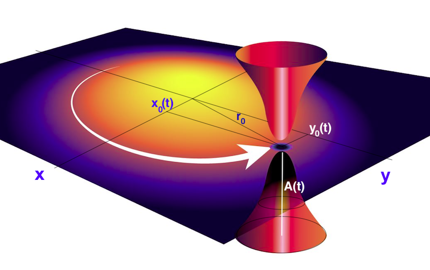
Figure 1: (color online) Graphical representation, in arbitrary units, of a bell-shaped laser stirring penetrable obstacle, with Gaussian format defined by (4) and (5)], circularly moving inside a BEC fluid with velocity $r_{0}\nu$ and radius $r_{0}$.

In the remaining part of this section, we first express the 3D GP equation (1) in dimensionless form, following by a reduction of the formalism to 2D, which is validated by a large aspect ratio $\lambda$. By keeping our notation close to the one used in Ref. Kumar2017 (for binary BEC with DDI), with the frequency and length units given by $\omega_{\rho}$ and $\ell_{\rho}\equiv\sqrt{\hbar/(m\omega_{\rho})}$, the full-dimensional variables are replaced by the corresponding dimensionless ones, as ${\bf r}/\ell_{\rho}\to{\bf r}$; $\omega_{\rho}t\to t$; $a_{s}/\ell_{\rho}\to a_{s}$; $\ell_{\rho}^{3/2}\Psi\to\Psi$. Also, by factoring the energy unit $\hbar\omega_{\rho}$, the trap interaction (3) and the stirring potential (4) will remain having the same formal expression, which means $V({\bf r},t)/({\hbar\omega_{\rho}})\to V({\bf r},t)$ and $A(t)/({\hbar\omega_{\rho}})\to A(t)$. Therefore, in dimensionless quantities, (1) is replaced by

$${\rm i}\frac{\partial\Psi({\mathbf{r}},t)}{\partial t} =\Big{(}-\frac{1}{2}\nabla^{2}+V({\mathbf{r}},t)+g|{\Psi({\mathbf{r}},{t})}|^{2}\Big{)}\Psi({\mathbf{r}},t)$$

$$+g_{\mathrm{dd}}\left[\int d^{3}{\mathbf{r}}^{\prime}{\displaystyle\frac{3\cos^{2}\alpha-1}{2|{\bf r-r^{\prime}}|^{3}}}|\Psi({\mathbf{r}}^{\prime},t)|^{2}\right]\Psi({\mathbf{r}},t),$$

where $g\equiv g_{3D}/(\hbar\omega_{\rho}\ell_{\rho}^{3})$ and $g_{\mathrm{dd}}\equiv N\mu_{0}\mu_{A}^{2}/(4\pi\hbar\omega_{\rho}\ell_{\rho}^{3})$. In terms of a defined dipole length $a_{dd}\equiv\mu_{0}\mu^{2}/(12\pi\hbar\omega\ell_{\rho}^{2})$, we can write $g_{dd}$ as $g_{dd}=3N(a_{dd}/\ell_{\rho})$. The stability of a dipolar BEC depends on the external trap geometry, e.g., a dipolar BEC is stable or unstable depending on whether the trap is pancake- or cigar-shaped, respectively. The instability usually can be overcome by applying a strong pancake trap with repulsive two-body contact interaction. The external trap helps to stabilize the dipolar BEC by imprinting anisotropy to the density distribution. So, with the dynamics of the dipolar BEC strongly confined in the axial direction ($\lambda\gg 1$), $\Psi({\bf r},t)$ can be decoupled as

$$\Psi({\bf r},t)\equiv\chi(z)\psi({\bf{\boldsymbol{\rho}}},t)\equiv\left(\frac{\lambda}{\pi}\right)^{{1}/{4}}\exp\left(\frac{-\lambda z^{2}}{2}\right)\psi({\bf{\boldsymbol{\rho}}},t),$$

where $\boldsymbol{\rho}\equiv(x,y)\equiv(\rho\cos\theta,\rho\sin\theta)$, allowing the dynamics in the $z-$direction be integrated out. This procedure is straightforward for non-dipolar BEC systems. However, we still need to perform the 2D reduction of the DDI configuration-space term, which is followed by the double $z-$integration. Apart of the DDI parameter $g_{dd}$, the 2D expression for the DDI is given by 2012Wilson

$$V^{(d)}(\boldsymbol{\rho}-\boldsymbol{\rho}^{\prime})=\int dzdz^{\prime}|\chi(z)|^{2}|\chi(z^{\prime})|^{2}\frac{3\cos^{2}\alpha-1}{2|{\bf r}-{\bf r}^{\prime}|^{3}}.$$ (7)

Given the corresponding Fourier transforms to the momentum space $({\bf k}_{\rho},k_{z})$, for this potential, being $\widetilde{{V}}^{(d)}({\bf k_{\rho}})$, for the axial density $\widetilde{n}({k_{z}})$, as well as for the 2D densities, ${\widetilde{n}}({\bf k_{\rho}})$, we have the following identification Kumar2019 :

$$\int d\boldsymbol{\rho}^{\prime}V^{(d)}(\boldsymbol{\rho}-\boldsymbol{\rho}^{\prime})|\psi^{\prime}|^{2}=\mathcal{F}_{2D}^{-1}\left[\widetilde{{V}}^{(d)}({\bf k_{\rho}}){\widetilde{n}}({\bf k_{\rho}})\right].$$ (8)

In the 2D momentum space, the DDI can be expressed as the combination of two terms, considering the orientations of the dipoles $\alpha$ and projection of the Fourier transformed in momentum space. One term is perpendicular, with the other parallel to the direction of the dipole inclinations 2012Wilson ; Zhang2016 , expressed by

$$h_{2d}^{\perp}(\mathbf{k}_{\rho}) = 2-3\sqrt{\frac{\pi}{2\lambda}}k_{\rho}\exp{\left(\frac{k_{\rho}^{2}}{2\lambda}\right)}{\rm erfc}\left(\frac{k_{\rho}}{\sqrt{2\lambda}}\right),$$ (9)

$$h_{2d}^{\parallel}(\mathbf{k}_{\rho}) = -1+3\sqrt{\frac{\pi}{2\lambda}}\frac{k_{x}^{2}}{k_{\rho}}\exp{\left(\frac{k_{\rho}^{2}}{2\lambda}\right)}{\rm erfc}\left(\frac{k_{\rho}}{\sqrt{2\lambda}}\right),$$ (10)

with ${\rm erfc}(x)$ being the complementary error function of $x$. For the parallel term, the projection of the polarizing field onto the $x-y$ plane is assumed in the $x-$direction. by considering that all directions $\theta_{k}$ are possible, and $k_{x}=k_{\rho}\cos\theta_{k}$ in (10), for a polarization field rotating in the $(k_{x},k_{y})$ plane, we can average $k_{\rho}^{2}\cos^{2}\theta_{k}$, replacing this term by $k_{\rho}^{2}/2$. By combining the two terms according to the dipole orientations $\alpha$, the total 2D momentum-space DDI, $\widetilde{{V}}^{(d)}({\bf k_{\rho}})=\cos^{2}(\alpha)h_{2d}^{\perp}(\mathbf{k}_{\rho})+\sin^{2}(\alpha)h_{2d}^{\parallel}(\mathbf{k}_{\rho})$, becomes proportional to $h_{2d}^{\perp}(\mathbf{k}_{\rho})$:

$${\widetilde{V}}^{(d)}({\bf k_{\rho}})=\frac{3\cos^{2}\alpha-1}{2}h_{2d}^{\perp}(\mathbf{k}_{\rho}).$$ (11)

Therefore, with the dipolar term in the Fourier-transformed momentum space, we obtain the effective 2D equation for the pancake-shaped dipolar BEC as

$${\rm i}\frac{\partial\psi}{\partial t} = \left\{-\frac{1}{2}\nabla_{\rho}^{2}+\frac{\rho^{2}}{2}+V_{G}+g_{s}|\psi|^{2}\right.$$ (12)

$$+ \left.g_{dd}\int\frac{d^{2}k_{\rho}}{4\pi^{2}}e^{i\mathbf{k}_{\rho}.\tilde{\rho}}\tilde{n}(\mathbf{k}_{\rho})\widetilde{{V}}^{(d)}({\bf k_{\rho}})\right\}\psi,$$

where $\psi\equiv\psi(\boldsymbol{\rho},t)$ is the 2D wave function, normalized to one, $g_{s}\equiv\sqrt{8\pi\lambda}{a_{s}N}/{\ell_{\rho}}$, and $V_{G}\equiv V_{G}(\boldsymbol{\rho},t)$ given by (4). In these dimensionless units, for a circular moving obstacle, we can conveniently write $V_{G}$ as

$$V_{G}(\boldsymbol{\rho},t) = A(t)\exp\left[-\frac{\rho^{2}+r_{0}^{2}-2\rho\,r_{0}\cos(\theta-\nu t)}{2\sigma^{2}}\right].$$ (13)

From this expression, we notice that the period $T$ for a complete one-loop circular movement (potential returning to the same value) is given by $T=2\pi/\nu$, such that we could replace $\nu t$ by $2\pi t/T$, with $t$ given in terms of the loop-period $T$. For the solution of the above Eq. (12), in order to investigate the vortex nucleation and dynamics of the vortex pair productions in the dipolar BECs, we need to combine the usual split-step Crank-Nicholson method with the Fast Fourier Transform approach Kumar2015 . In our numerics, we have used a $256\times 256$ grid size with $\Delta x=\Delta y=0.1$ for both $x$ and $y$ (units $\ell_{\rho}$), with time step $\Delta t=0.0001\omega_{\rho}^{-1}$. Further, we have confirmed that the results are not affected by doubling the aforementioned grid sizes and grid spacing. Along with our study, we also kept fixed the following parameters related to the atom-atom interactions and stirring Gaussian model: $a_{s}=50\,a_{0}$, $a_{dd}=66\,a_{0}$, $N=1.5\times 10^{4}$, $A_{0}=36\hbar\omega_{\rho}$, $r_{0}=3.5\ell_{\rho}$, and $\sigma=1.5\ell_{\rho}$, where $a_{0}=5.29177\times 10^{-11}m$ is the Bohr radius and $\ell_{\rho}=1\times 10^{-6}m$. The choice of these parameters is motivated by possible experimental realization considering the dipolar ¹⁶⁸Er, with two-body scattering length enough repulsive such that the effect of the dipolar interaction can better be evaluated by changing the tilting DDI angle $\alpha$. The radial position of the obstacle ($r_{0}$) inside the condensate was arbitrarily chosen at an approximate average distance between the center and the border limits of the condensate, considering that the critical velocities for the production of vortex-pairs are given by $v_{c}=r_{0}\nu_{c}$. By varying the $r_{0}$ position inside the main part of the condensed fluid, one can verify that no vortex pairs can be produced when $r_{0}\to 0$.

III Vortex nucleation by stirring Gaussian potential

This section is concerned with the dynamical production of vortex dipoles and vortex clusters by the time-dependent stirring interaction. To obtain a stable ground state density profile, in our simulations the Eq. (12) is first solved by using imaginary time $(t\rightarrow{-it})$, without the Gaussian obstacle ($A(t)=0$). Next, this solution is evolved in real-time with the obstacle ($A(t)\neq 0$). Once considered fixed the shape of the Gaussian model for the obstacle (amplitude and width), with its radial position inside the condensate, the principal model parameters are the strength of the DDI and the angular frequency $\nu$ of the obstacle, implying in a corresponding linear velocity $v=\nu r_{0}$. We have considered two types of simulations, with the type-II ($\varepsilon\neq 0$) differing from type-I ($\varepsilon=0$) by additionally verifying the effect of vibration (with frequency $\omega_{A}$) in the amplitude of the obstacle.

III.1 Critical velocities: Phase diagrams

With the circular movement of the obstacle fixed at a constant radial position $r_{0}$, the numerical simulation starts (at $t=0$) with a linear ramping of the time-dependent amplitude $A(t)$ of the stirring interaction, from $A(t)=0$ to $A(t)=A_{0}$, within the time interval $\Delta T=0.0025\omega_{\rho}^{-1}=25\Delta t$. Along the simulation, this value $A_{0}$ remains fixed in case of type-I model, being time vibrating with frequency $\omega_{A}$ in case of type-II model. The obstacle inside the condensate is assumed moving with a constant frequency $\nu$, Once considered the model interaction parameters, as the two-body contact $a_{s}$ and dipole-dipole strength (provide by $a_{dd}$ and the angle $\alpha$, our results for the two defined stirring models, related to the production of vortex-antivortex pairs and vortex clusters, are resumed in the two panels shown in Fig. 2, in which we are providing diagrams for the DDI angles $\alpha$ as functions of the rotation frequency $\nu$ ($v=r_{0}\nu$). The panels (a) and (b) are, respectively, for non-breathing ($\varepsilon=0$ ) and breathing ($\varepsilon=0.4$ with $\omega_{A}=2\omega_{\rho}$) modes of the Gaussian obstacle. Also, in the time-dependent expression of the amplitude (5), we assume $A_{0}=36\hbar\omega_{\rho}$ (which is about $90\%$ of the chemical potential $\mu$) and $\sigma=1.5\ell_{\rho}$. Considering such moving penetrable obstacles, the vortices are created in the form of dipoles consisting of two vortices with opposite circulations, within a dynamical process qualitatively different from the typical hard cylinder case, where vortices can also be generated individually due to the vortex pinning effect in the density-depleted region Lim2022 . Within this process, for fixed values of $\alpha$, critical velocities can be verified for the production of vortex-antivortex pairs, or vortex clusters, defining three regions: with no vortex (A), with vortex-antivortex pairs emerging in distinguishable time-gap intervals (B), and with vortex pairs emerging as clusters (in indistinguishable time intervals, almost simultaneously). In the panels of Fig. 2, considering the given fixed parameters, the separation between regions A and B is provided by solid-thick lines, that interpolate precise numerical results (showing by stars in case of type-I model). By increasing even more the frequency $\nu$, another critical border transition can be approximately verified, when the vortex pairs start emerging as clusters. Panel (a) shows more explicitly how the vortex pairs produced in the first cycle ($N_{v\bar{v}}$) change by increasing $\nu$. The first thick-solid line ($N_{v\bar{v}}=1$, for $\alpha$ versus $\nu$) is interpolating exact critical points obtained in our calculation, represented by stars. The other long-dashed lines are guiding eyes for the verified crescent $N_{v\bar{v}}$ as $\alpha$ increase with $\nu$.

The dynamical process of the vortex nucleation can be understood as follows: When the Gaussian obstacle moves faster than a critical velocity $v_{c}$, energy is transferred into the BEC density by changing the superfluid velocity field near the obstacle. As the accumulated energy $E$ exceeds a certain threshold $E_{v}$, the energy will dissipate via vortex-antivortex emission Lim2022 , represented by the thick-solid line between regions A and B, as described above; or via vortex-antivortex clusters for even larger velocities of the obstacle. Further, a remark has to be done related to the observed number of pairs $N_{v\bar{v}}$ in our simulations: once the vortex dipoles are produced in the first cycle, by keeping the same rotational speed the number of vortices produced in the next cycles is clearly reduced, which can be explained by the changes in the fluid dynamics as the time flows. The production of vortex pairs occurs more easily with the obstacle rotating inside an originally stationary uniform fluid. As the time flows, the fluid near the obstacle is not anymore in the same stationary state as it happens when starting the first loop. For different combinations of dipolar and contact interactions, a more detailed analytical investigation on this dynamics is being under consideration in a following related work, in which the plan is to investigate the interaction between the produced vortex pairs and their persistency inside the fluid.

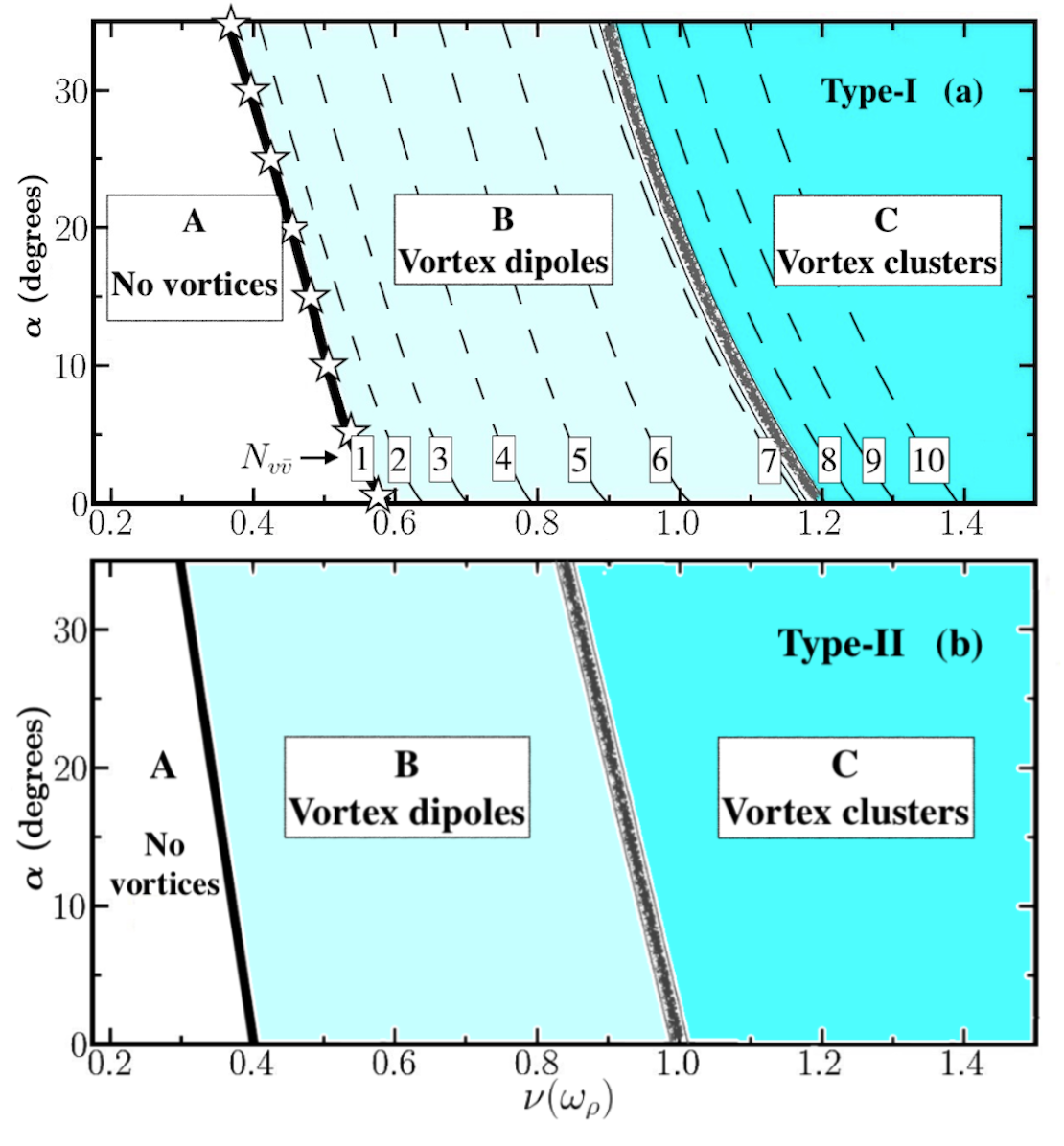
Figure 2: (color online) Diagrams for $\alpha$ (angles for DDI strengths) versus $\nu$ (rotational frequencies) for type-I (a) and type-II (b) models, described by (4), with $\varepsilon=0$ (a) and $(\varepsilon,\omega_{A})=(0.4,2\omega_{\rho})$ (b) (with $A_{0}=36\hbar\omega_{\rho}$ and $\sigma=1.5\ell_{\rho}$ in both cases). The critical rotational frequencies for emergence of the first vortex pair are given by the thick solid lines separating regions A and B. With type-II following a behavior similar as type-I, panel (a) shows more explicitly how the critical $\nu$ for $N_{v\bar{v}}=1$ is obtained by interpolating exact results (indicated by stars). The long-dashed lines are for increasing number of vortex pairs, as indicated. The separation between regions B (vortex dipoles) and C (vortex clusters) is represented by a blurred band line in both panels. Other common parameters are: $r_{0}=3.5\ell_{\rho}$ (obstacle location), $a_{s}=50\,a_{0}$, $a_{dd}=66\,a_{0}$, and $N=1.5\times 10^{4}$.

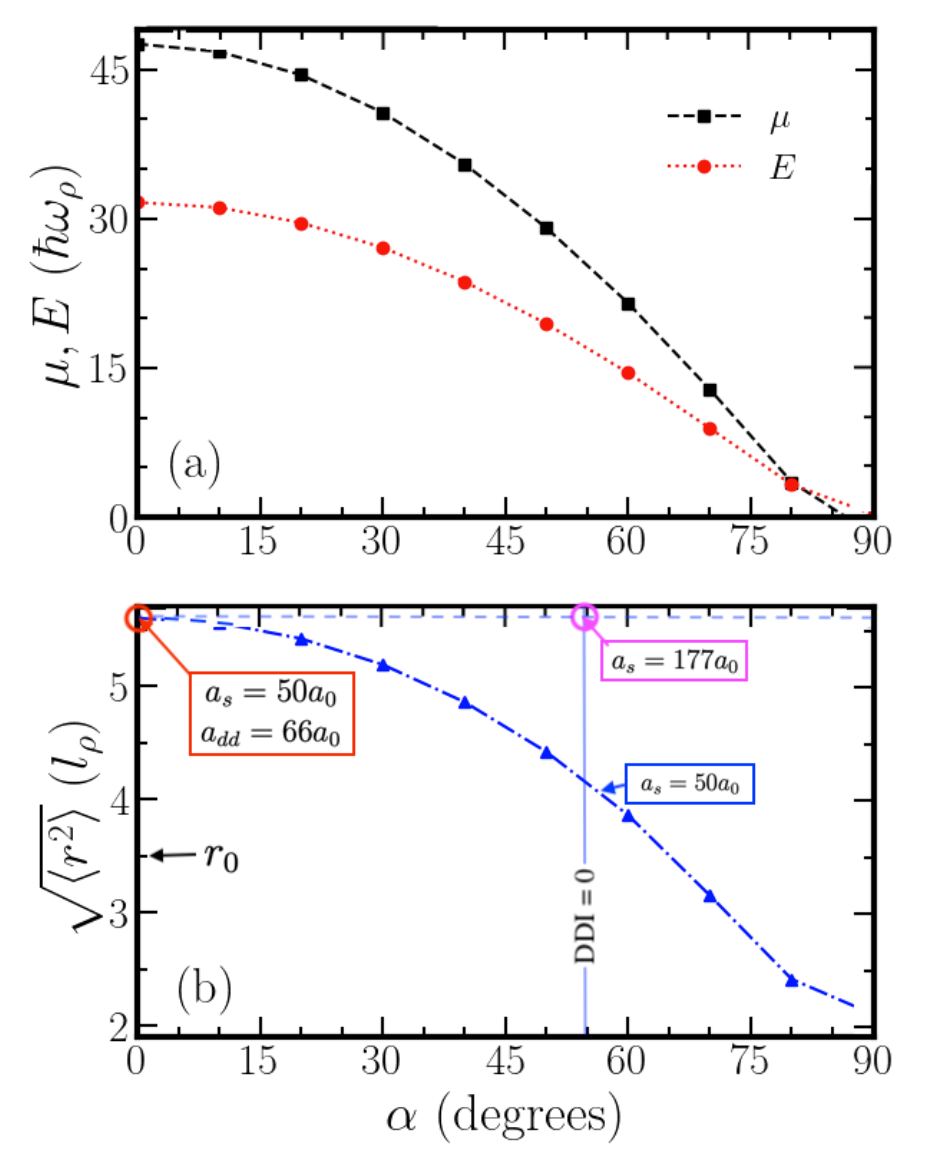
Figure 3: (color online) Effect of DDI ($\alpha$) variations on the ground-state chemical potential ($\mu$) and energy ($E$) are shown in (a), with the corresponding rms radius ($\sqrt{\langle r^{2}\rangle}$) in (b). For $\alpha<54.7^{\circ}$ the DDI is repulsive, whereas for $\alpha>54.7^{\circ}$ it is attractive. The two indicated circles in (b) refer to the necessary change in the contact interaction $a_{s}$ to keep the respective condensed clouds with about the same size.

By examining in more detail the type-I model [panel (a) of Fig. 2], when the repulsive DDI is at the maximum ($\alpha=0$), the minimum critical frequency to produce one pair in the first cycle ($N_{v\bar{v}}=1$) is verified being $\nu_{c}\approx 0.57\omega_{\rho}$, with the number of pairs increasing almost linearly up to $\nu\approx 1.2\omega_{\rho}$, when the vortex-cluster productions start to occur (with more than one pair at each instant of time). For the type-II case, as shown in panel (b) of Fig. 2, the critical frequency to producing vortex dipoles at $\alpha=0^{\circ}$ is $\nu_{c}\approx 0.4\omega_{\rho}$, with $N_{v\bar{v}}$ increasing with $\nu$ up to $\approx 1\omega_{\rho}$ when the pairs start being produced as clusters. The shifted region borders to lower values of $\nu$ (by going from type-I to type-II models) are consistent with the extra dynamics due to the amplitude vibration. By reducing the repulsive DDI, with increasing $\alpha^{\prime}$s, in both cases $\nu_{c}$ is consistently reduced, as shown for $\alpha$ going from 0^∘ to 35^∘. In fact, this behavior is expected considering the other parameters that are kept fixed. With the condensate size being reduced (as the contact interaction remains at $a_{s}=50a_{0}$), the radial position of the moving obstacle, fixed at $r_{0}=3.5\ell_{\rho}$, end up being located in relatively less-dense region of the condensate.

In all given numerical simulations represented in Fig. 2, except for the Gaussian amplitude and DDI angle, the other parameters are kept fixed, with the trap aspect ratio $\lambda=100$, interaction strengths ($a_{dd}=66a_{0}$ and $a_{s}=50a_{0}$) and the number of atoms $N=1.5\times 10^{4}$, as indicated in the caption of Fig. 2. Here, we should remind that the assumed magnetic moment, $\mu_{A}=7\mu_{B}$, implies ¹⁶⁸Er or ¹⁵¹Eu (with the corresponding change in the mass unit) as the atomic sample, such that the angle $\alpha$ must be correspondingly shifted when considering another dipolar species (as ¹⁶⁴Dy or ⁵²Cr). The critical velocities ($r_{0}\nu_{c}$) are verified being approximately constant for reasonable changes of $r_{0}$ inside the condensate, such that no vortex pairs are produced near $r_{0}=0$.

The results shown in Fig. 3, for the chemical potential $\mu$ and total energy $E$, [panel (a)], with the corresponding root-mean-square (rms) radius [panel (b)], as functions of the DDI angle $\alpha$, without the Gaussian obstacle, are helpful to estimate the more convenient radial position for the obstacle in the following simulations with the obstacle. As verified, by inspecting both panels (a) and (b), the rate of changing for $\mu$ is approximately the same as the rate of changing for $\langle r^{2}\rangle$. As the position of the obstacle approaches the center, the frequency $\nu$ needs to increase, such that for $r_{0}\to 0$ no vortex can be created by the stirring. Therefore, in principle, one could conclude that larger values of $r_{0}$ will be more favorable for the production of vortex dipoles or vortex clusters, implying the obstacle located in the low-density region of the trap. However, this possible choice will bring us the role of the other constraints we have to consider, such as the contact atom-atom interaction. By assuming fixed and repulsive $a_{s}=50a_{0}$, the DDI parameter $\alpha$ is controlling the size (and corresponding the chemical potential) of the condensate. So, we need to keep the DDI enough repulsive ($\alpha<\alpha_{M}$), otherwise with $\alpha>\alpha_{M}$ the stirring position will be located in the too-low density region, or even outside the condensate, as one can verify by considering $\alpha\geq 70^{\circ}$, when the rms radius of the condensate becomes smaller than $r_{0}$. With these concerns, restricted by the parameter regions in our study of vorticity, $\alpha$ was chosen enough smaller than the magic angle $54.7^{\circ}$.

As to keep the study of the dynamics in similar conditions, considering the size of the condensed cloud, with $\mu$ and $\langle r^{2}\rangle$ not deviating more than about 20% from their maximum values by varying the interaction parameters (contact and DDI), we have verified as appropriate to keep the DDI limited to the repulsive region, with $\alpha$ between $0^{\circ}$ and 35^∘. This, obviously, restricted by the other model parameters that are kept fixed in our study, such as the contact interaction and position of the obstacle. By going to attractive DDI region, in order to maintain the size of the condensate in stable conditions, as well as not too small considering the position of the obstacle, one needs necessarily to increase the repulsive contact interaction, such as going to $a_{s}=177a_{0}$, as shown in Fig. 3(b). As an alternative, for a smaller stable cloud, one could reduce the radial position of the obstacle. Following our vortex dynamics study, in the next subsection, a comparative analysis is also provided in section III.B for two condensates with equivalent rms and $\mu$, with the DDI of one of the condensates reduced to zero.

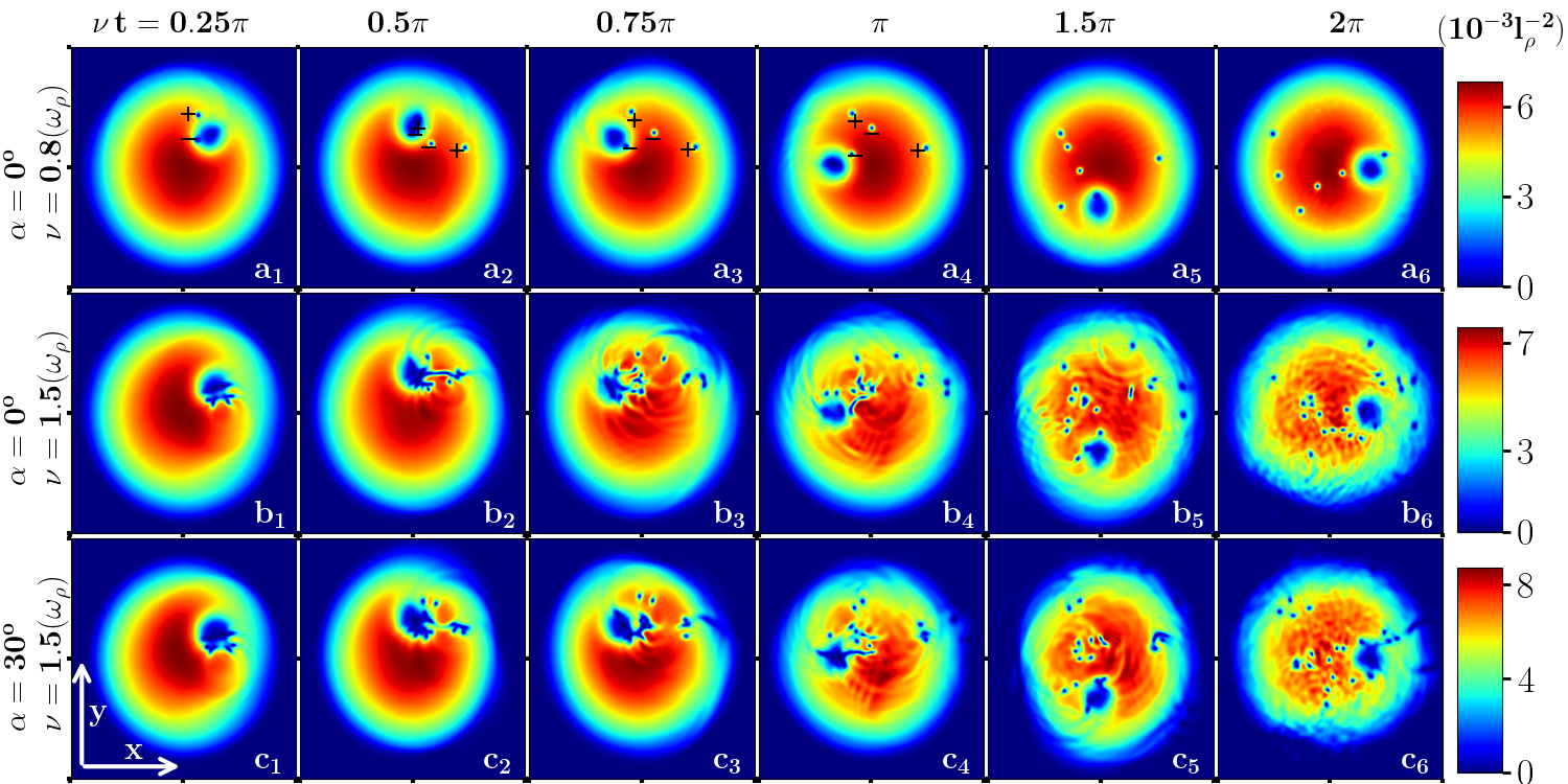
Figure 4: (color online) For the type-I ($\varepsilon=0$) rotating obstacle at $r_{0}=3.5$, this figure shows time snapshots of full-numerical results for the 2D densities (levels indicated by color bars), with the production of vortex-antivortex (upper row) and vortex-cluster (middle and lower rows), in the first cycle, as indicated: $\nu t=\pi/4$ (a₁,b₁,c₁) till $\nu t=2\pi$ (a₆,b₆,c₆). The rotation frequencies and DDI angles are, respectively, $(\nu,\alpha)=(0.8\omega_{\rho},0^{\circ})$ (top row), $=(1.5\omega_{\rho},0^{\circ})$ (middle row), and $=(1.5\omega_{\rho},30^{\circ})$ (bottom row). Other fixed parameters (not explicitly indicated) are the same as the ones given in the caption of Fig. 2. The vortex $(-)$ and antivortex $(+)$ signs are indicated in the first four panels of the upper row, respectively.

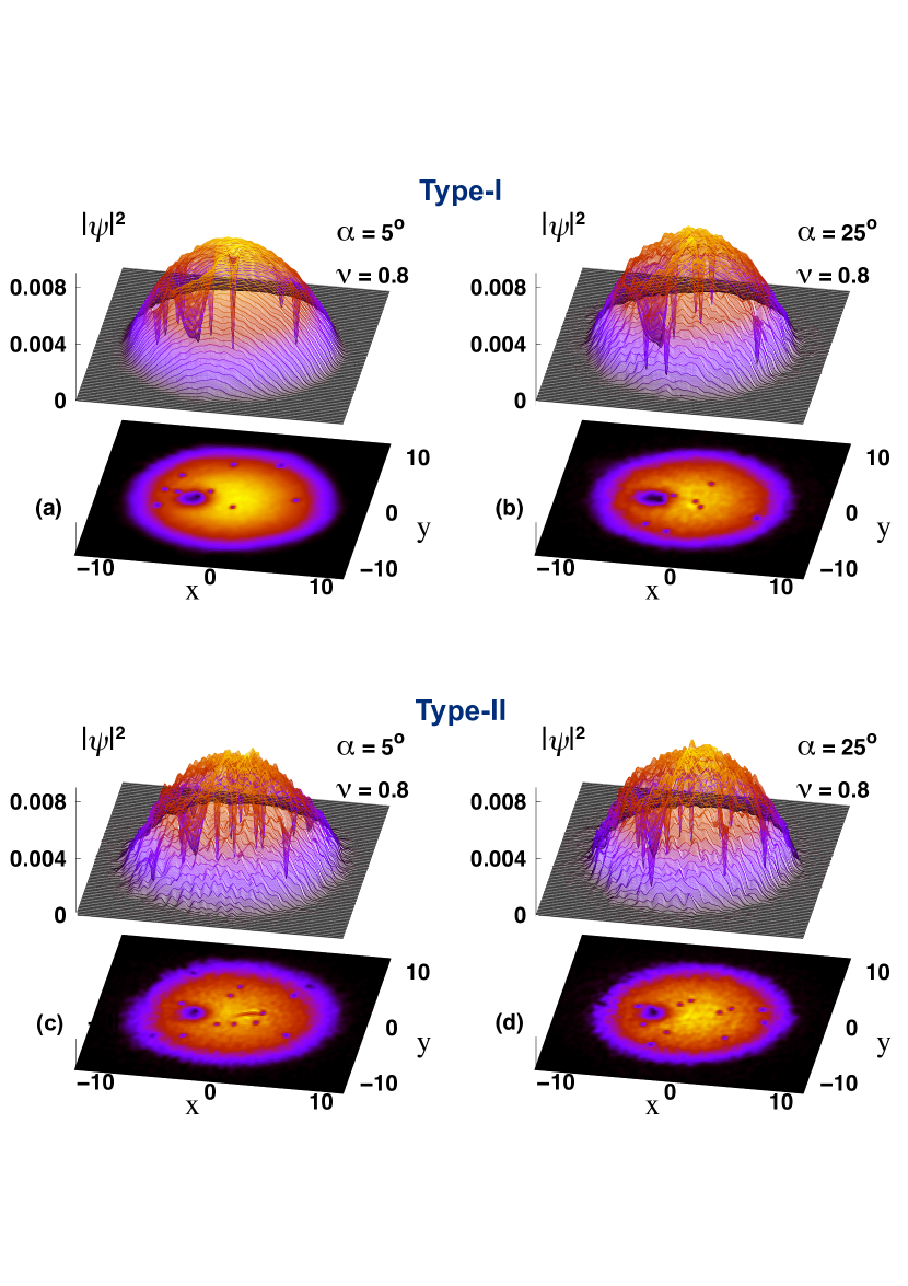
Figure 5: (color online) Results obtained for the 2D densities ($|\psi|^{2}$, in $l_{\rho}^{-2}$ units), given in 3D plots, with corresponding projections in the $x$ and $y$ plane (units $\ell_{\rho}$), for type-I [$\varepsilon=0$, panels (a) and (b)] and type-II [$(\omega_{A}=2\omega_{\rho},\varepsilon=0.4$, panels (c) and (d)] models. We consider two sets of DDI angles $\alpha=5^{\circ}$ [panels (a) and (c)] and $25^{\circ}$ [panels (b) and (d)], with fixed rotational frequency ($\nu=0.8\omega_{\rho}$), as indicated. They are representing the vortex-antivortex production in region B (shown in Fig. 2), with identical arbitrary time such that $\nu t$ is slightly larger than $3\pi$. The other parameters are, respectively, the same as given in the caption of Fig. 2.

III.2 Vortex dynamics within the condensate

In this section, we select some specific parameters for which we can verify more clearly the associated dynamics in the formation of the vortex-antivortex pairs, by following the evolution of the densities. The differences between the two types of stirring approaches rely only on the additional dynamics introduced by a periodic variation in the amplitude g of the stirring interaction, given by (5). In view of that, we can first resume our main results for the case in which the amplitude is kept constant, followed by an analysis of the type-II case (when the amplitude is vibrating). For this purpose, we present Fig. 4 considering the type-I model, immediately followed by the corresponding discussion for the type-II model, in order to verify possible additional effects (if any) introduced by the periodic vibration of the stirring amplitude.

Figure 4 shows three rows of snap-shot density plots obtained from full-numerical calculations considering the type-I Gaussian model for the stirring. These results illustrate the nucleation of the vortex dipoles and vortex clusters during the movement of the non-breathing penetrable Gaussian obstacle with two different frequencies ($\nu=0.8\omega_{\rho}$ and $1.5\omega_{\rho}$) and two DDI angles ($\alpha=0^{\circ}$ and 30^∘). The Gaussian obstacle with its position is represented in each of the panels by the hollow (minimum density) moving anti-clockwise inside the fluid. In the upper row of panels, for $\nu=0.8\omega_{\rho}$, which is picked from region B in Fig.2(a), the Gaussian obstacle nucleates the vortices in the form of vortex dipoles. The nucleation starts close to $t=1\omega_{\rho}^{-1}$ [or $\nu t=\pi/4$, as verified in panel (a₁)]. In the other two rows, for $\nu=1.5\omega_{\rho}$, which are picked from region C in Fig.2(a), the Gaussian obstacle nucleates the vortices in the form of clusters. In these cases, with two different DDI angles, the nucleation starts before, close to $t=0.5\omega_{\rho}^{-1}$ [or $\nu t=\pi/4$, as verified in panels (b₁) and (c₁)].

In order to appreciate how the vortex-antivortex, as well as clusters of vortex, are emerging, we are showing six snapshots for the first cycle, with $\nu t$ going from $\pi/4$ up to $2\pi$. As verified in the first row, with $\alpha=0^{\circ}$ and $\nu=0.8\omega_{\rho}$, we have the production of about three vortex-antivortex pairs within a cycle. For the stirring model, a constant amplitude $A_{0}=36\hbar\omega_{\rho}$ is assumed in this case. More specifically, the first row [$\nu=0.8\omega_{\rho}$, with $\alpha=0^{\circ}$] corresponds to region B of the upper panel of Fig. 2, with the vortex-antivortex pairs being produced regularly at different time intervals, as the obstacle moves anti-clockwise around the circle. The second and third rows refer to the vortex-cluster production region C in the upper panel of Fig. 2, with $\nu=1.5\omega_{\rho}$ and $\alpha=0^{\circ}$ (second row) and $30^{\circ}$ (third row), when vortex clusters are being produced (more than one pair at each time interval). Corresponding to $\nu=0.8\omega_{\rho}$ and $1.5\omega_{\rho}$, the respective stirring velocities are $v=2.8$ and $v=5.25$. They are selected in correspondence with the results previously shown in the upper panel of Fig. 2. The effect of the rotation $\nu$ can be seen by comparing the first with the second row, as $\nu$ is changed to $1.5\omega_{\rho}$ with $\alpha$ having the same value. Similarly, to see the effect of $\alpha$, we consider the case with $\nu=1.5\omega_{\rho}$, with the second and third row varying $\alpha$ from 0^∘ to $30^{\circ}$. In this case, the difference is quite visible in the contour plots of the densities, as well as the dynamics of the emerged vortex and antivortex. Reflecting the fact that the repulsive DDI for $\alpha=0^{\circ}$ is stronger than for $\alpha=30^{\circ}$, we can observe that the vortex-antivortex pairs repeal each other more strongly in case that $\alpha=0^{\circ}$ [compare, for example, the positions of the emerged vortices in (b₄) with the ones in (c₄)].

One should notice that, differently from the case in which the obstacle moves linearly inside the condensate Sabari2018 , the production of the vortex-antivortex pairs occurs with each vortex of the pair emerging at a slightly different time. This can be understood considering that the density distribution of the BEC fluid around the obstacle is not the same in both sides. Within a counter-clockwise stirring rotation, as the fluid is denser in the internal left side, the emerging vortex [indicated by ($-$) in panels (a₁-a₄) of Fig. 4] takes a slightly longer time to emerge than the associated antivortex [indicated by ($+$)].

Considering the type-II model, according to the results previously pointed out in Fig. 2 for the critical rotational velocities necessary for vortex-antivortex productions, due to the additional dynamics introduced by the amplitude vibration, more vortex pairs are verified emerging in a cycle than the ones observed in Fig. 4. These results can already be verified by examining the two diagrams shown in Fig. 2. For the type-II case, considering $A_{0}=36\hbar\omega_{\rho}$ and $\varepsilon=0.4$, the amplitude is vibrating from $A=21.6$ [when $\sin(\omega_{A}t)=-1$] till $A=50.4$ [when $\sin(\omega_{A}t)=1$]. With $\omega_{A}=2\omega_{\rho}$ the oscillating period is $5/2$ times the stirring cycle frequency, when $\nu=0.8\omega_{\rho}$; and $4/3$ in case $\nu=1.5\omega_{\rho}$. Therefore, the production of vortex pairs and vortex clusters occurs at shorter time intervals in the case of the type-II model, as the quantum fluid is more affected by the Gaussian amplitude vibration.

By verifying that the results for the densities are not significantly different in both cases, in Fig. 5 we have selected parameters considering the region B of Fig.2, with rotational frequency $\nu=0.8\omega_{\rho}$, presenting our results in a 3D illustrative format, for the dynamics observed without (type-I) and with (type-II) amplitude vibration. The choice of the two DDI angles have the purpose of verifying how the dynamical behavior of the produced vortex pairs is changed by going from a more repulsive $\alpha=5^{\circ}$ to a less repulsive $\alpha=25^{\circ}$ condition. The panels (a) and (b) refer to the type-I (non-breathing mode, $\varepsilon=0$), with panels (c) and (d) referring to the type-II [breathing mode, with ($\omega_{A},\varepsilon)=(2\omega_{\rho},0.4)$]. In both cases, we select identical time snap-shots, with $\nu t$ slightly larger than $3\pi$ (second loop). By comparing the left with the right panels, in both cases, the obstacles (radially fixed at $r_{0}$) are moving inside regions of the respective condensates that have relatively slightly different densities: It is in a denser region in case $\alpha=5^{\circ}$, because the radius is larger than for $\alpha=25^{\circ}$. In other words, by keeping fixed the radius $r_{0}$, to study the dynamics within similar conditions we need to restrict the values of the DDI to reasonable not too large angles, such that the obstacle remains moving in similar density regions of the condensate. By taking larger values of $\alpha$ the system will be more attractive (unless, to compensate, we change another interaction parameter, as the scattering length) with the obstacle position moving at too low density region (as close to the radial border limits) of the condensate. As comparing with Fig. 4, where we choose $\alpha=0^{\circ}$ and $\alpha=30^{\circ}$, the motivation in changing slightly the angles, as shown in Fig. 5, is to appreciate how the vortices are emerging by slightly decreasing the DDI (with $\alpha$ going from 0$\circ$ to 5^∘) or slightly increasing (with $\alpha$ going from 30^∘ to 25^∘).

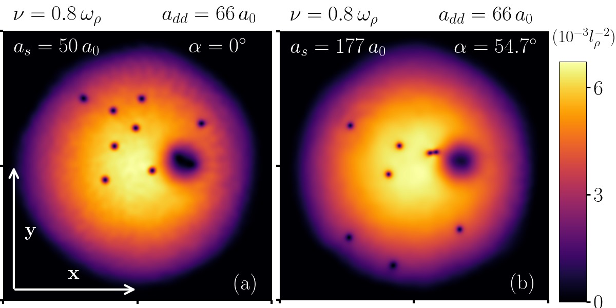
Figure 6: Snap-shots of densities obtained with maximum DDI ($\alpha=0$, at left) and without DDI ($\alpha=\alpha_{M}=54.7^{\circ}$, at right) obtained near two cycles ($4\pi$). At right $a_{s}=177a_{0}$, in order to have both clouds with about the same rms radius. A corresponding gif-movie animation is presented in a Supplemental Material.

III.3 Role of DDI in the dynamics

For a comparative study on the role of DDI for the vorticity and turbulence, we need to consider two condensates such that one of them is without DDI. For that, by starting with a simulation in which $a_{s}=50a_{0}$, the maximum DDI is obtained at $\alpha=0$, as indicated by the red circle inside Fig. 3(b). As to compare with this case, in the other simulation we consider $\alpha$ fixed at the magic angle, implying the DDI is zero. But, as we need to consider condensates with about the same radial extension, such that the obstacle position will be not in the low-density region, we have to assume a larger value $a_{s}=177a_{0}$ in order to have both condensates with about the same sizes. This second case is indicated by a magenta circle inside Fig. 3(b). Resulting from this comparative simulation, we have two snap-shots in Fig. 6, which are taken when the rotation finish two cycles (4$\pi$). By looking to the dynamics from $t=0$, in both cases (with and without DDI) we observe that the initial production of vortices occurs in a very similar way (slightly faster in case of DDI), implying that the critical velocities verified in Fig. 2 are mainly due to the changes in chemical potential and rms radius. However, after the first cycle it is also visible in the dynamics that the case with $\alpha=0$ (maximum DDI) presents stronger fluctuations in the cloud, absent for non-dipolar case, reflecting the different characteristics of the interactions in the fluid. In fact, a more close inspection by varying the rotation speed $\nu$ of the obstacle, considering two extreme cases with equivalent condensed cloud sizes, one in which the DDI is zero (pure contact interactions with $a_{s}=177a_{0}$), with the other in which the contact interaction is zero (pure DDI, with $a_{dd}=91a_{0}$ and $\alpha=0$), it was verified that the production of vortex-antivortex requires smaller rotation speed in case of pure DDI.

In a Supplemental Material DDIvsContact-animation , we include explicitly our results obtained for the dynamics, with $\nu=0.8\omega_{\rho}$, through an animation in which we can observe the time evolution of both condensed systems in the process of vortex-antivortex emission, with ($\alpha=0$) and without ($\alpha=\alpha_{M}$) DDI, from $\nu t=0$ till $\nu t=2\pi$. When removing the DDI, the contact interaction has to be redefined (from $a_{s}=50a_{0}$ to $a_{s}=177a_{0}$) in order to maintain both condensates having about the same size, with the obstacle kept fixed at $r_{0}=3.5\ell_{\rho}$. Still, the similarity of the two cases when started the dynamics with the obstacle is indicating that the kind of interactions (contact or DDI) are not so relevant for the initial formation of the vortex-antivortex pairs in the condensate, provided that both densities are initially found in the same conditions, having about the same sizes. As the number of vortex pairs being created as time flows is drastically reduced, within this comparison, one can draw the conclusion that the vorticity and turbulence are mainly affected by the size of the condensed cloud, instead of the two kind of interactions we are considering (DDI or contact). However, apart of the initial vortex production, in view of the different observed dynamics inside the fluid, a more dedicated conclusive investigation may be required. As the results we are reporting rely only on the numerical solution of the corresponding circular-stirred GP formalism with two-body contact and dipolar interactions, without the assumption of possible beyond mean-field corrections, a more prospective analysis may not be difficult, but outside the scope of the present work.

IV Spectral dynamics and quantum turbulence in stirred BEC with DDI

Our aim in this section is to characterize the possible emergence of turbulent behavior in the dipolar condensate, by full-numerical investigation of the evolution and behavior of the vortices within a spectral analysis. The results of our study are illustrated by selecting two different rotational frequencies of the obstacle (considering the regions B and C in the two panels of Fig. 2), with repulsive DDI strengths being typified by two distinct angles $\alpha$. In particular, the choice to keep the DDI enough repulsive was determined by the other choices for the model parameters, such as the contact interaction and radial position of the circularly moving obstacle.

Towards an understanding of possible quantum turbulence in a quantum fluid as a cold-atom system described by the mean-field GP theory, one of the main characterization to look for is the Kolmogorov’s classical scaling law $k^{-5/3}$ in the incompressible kinetic energy spectrum Kolmogorov , as pointed out in several works and reviews in this direction Barenghi2001 ; Tsatsos2016 ; Madeira2020b . As reported already in 1997 in Ref. Nore1997 , considering nonlinear Schrödinger equation solutions with possible implications in experiments for Helium superfluid, it was found that low-temperature superfluid turbulence follows approximately Kolmogorov’s scaling. The vorticity dynamics of the superflow were shown to be similar to that of the viscous flow, including vortex reconnection. Directly connected with cold-atom experiments in the last 15 years, vorticity and QT was reported in oscillating BECs in Refs. Henn2009 ; Henn2010 . In nonuniform BEC the occurrence of QT was investigated numerically in Ref. Horng2009 . The actual increasing interest in the QT investigations in cold-atom physics can be traced from Refs. White2010 ; Seman2011 ; Reeves2012 ; Kwon2014 ; White2014 ; Fujimoto2015 ; Cidrim2016 ; Kobayashi2021 ; Reeves2022 , having as strong motivating factor possible links between QT and its classical counterpart. Therefore, by assuming the Kolmogorov scaling behavior of the kinetic energy spectrum as a parameter for a universal description of turbulence, one has to characterize the length scales by considering the necessary stationary states with enough number of vortices being produced. For the analysis of vorticity and the occurrence of turbulence in an ensemble of particles, the relevant quantity is the associated kinetic energy, which can be decoupled in two terms, considering the compressibility. The key concepts concerned with the energy spectra of vortex distributions in 2D QT, together with a discussion on similarities and differences with 2D classical turbulence has been explored for homogeneous compressible superfluid in Ref. 2012Bradley . For our present analysis of the energy spectra, in the next we follow some details provided more recently in Refs. 2022Bradley ; 2023daSilva . Of particular interest in our case is the investigation of a dipolar confined BEC system, which is under external laser stirring periodic perturbation.

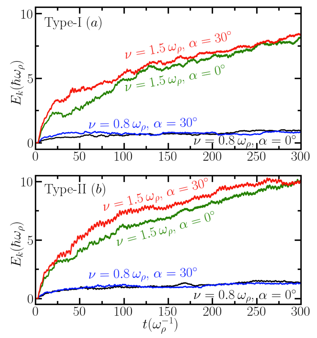
Figure 7: (Color online) Time evolutions of the total kinetic energies for the type-I [panel (a)] and type-II [panel (b)]stirring models. In both the cases, the results are for two sets of rotational velocities ($\nu=0.8\omega_{\rho}$ $1.5\omega_{\rho}$) and DDI $\alpha$ angles ($\alpha=0^{\circ}$ and $30^{\circ}$), as indicated close to the respective lines.

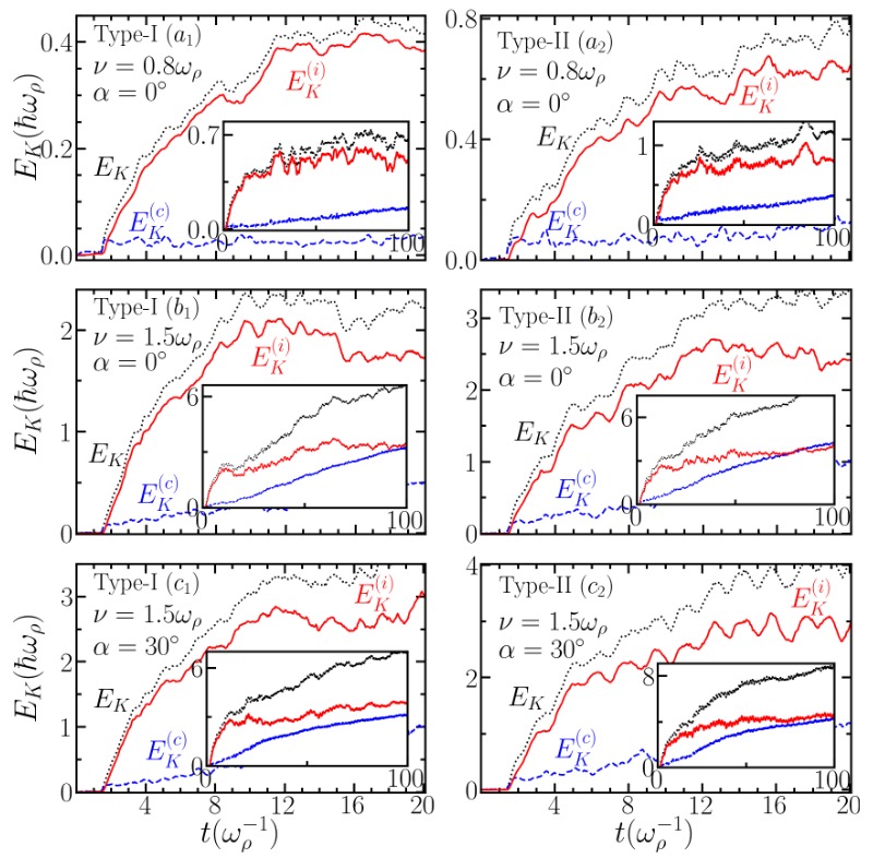
Figure 8: (Color online) Time evolution of the total ($E_{K}$, black-dotted lines), compressible ($E_{K}^{(c)}$, blue-dashed lines), and incompressible ($E_{K}^{(i)}$, red-solid lines) kinetic energies (in $\hbar\omega_{\rho}$ units) for type-I (left panels) and type-II (right panels) stirring motion of the Gaussian obstacle. The rotational frequencies $\nu(=0.8\omega_{\rho},1.5\omega_{\rho})$ and DDI angles $\alpha(=0^{\circ},30^{\circ})$ are indicated inside the respective panels. The insets are shown the corresponding long-time behaviors. The time intervals, identified in the bottom panels, are common to all panels.

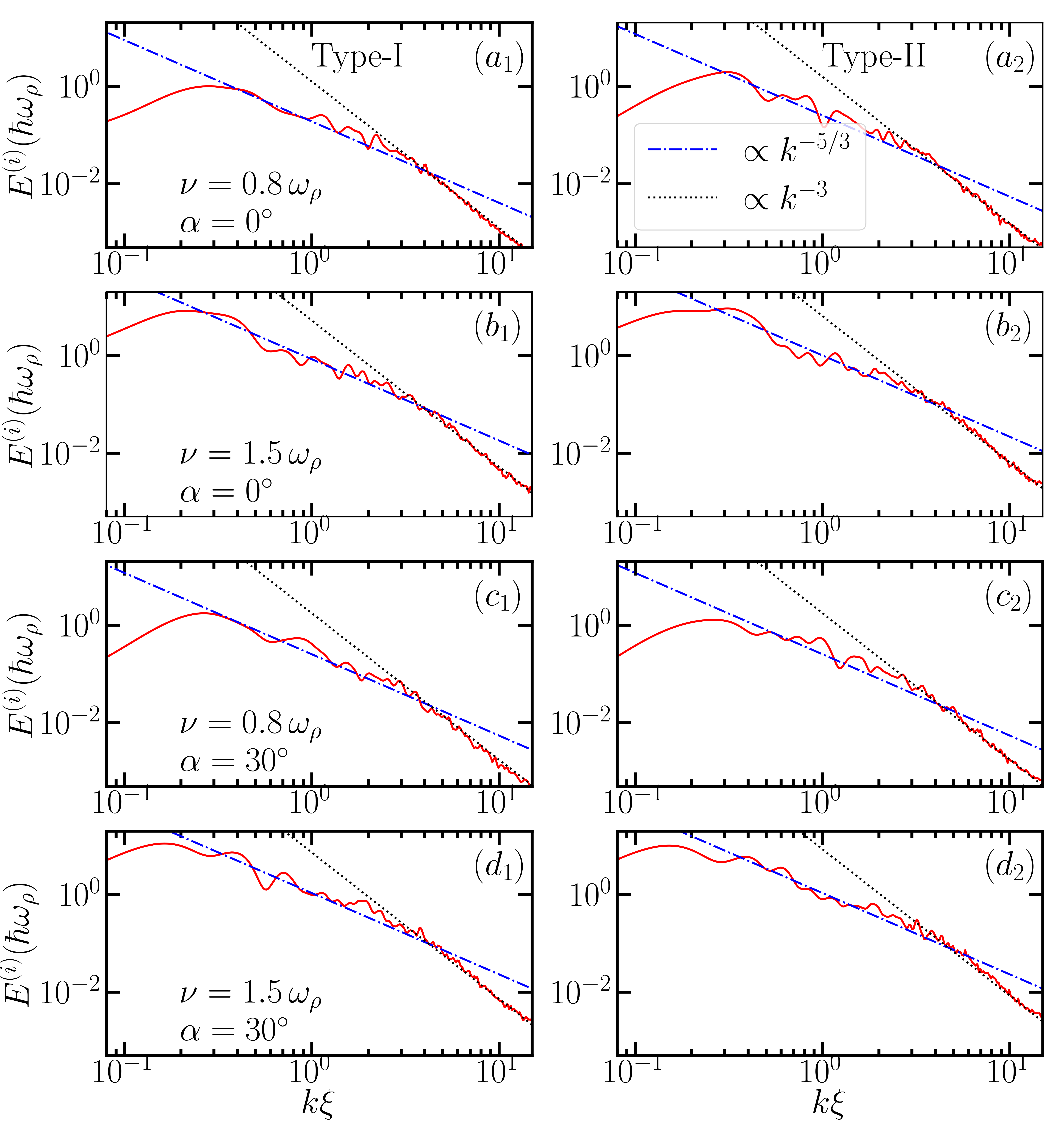
Figure 9: Incompressible kinetic energy spectra, $E^{(i)}(k)$, obtained for the type-I [(a₁)-(d₁) panels] and the type-II [(a₂)-(d₂) panels] models, as functions of the dimensionless $k\xi$ (where $\xi$ is the healing length). The rotation frequencies $\nu$ (0.8$\omega_{\rho}$ and 1.5$\omega_{\rho}$) and DDI angles $\alpha$ ($0^{\circ}$ and $30^{\circ}$) are being indicated inside the respective panels. At each panel, the $E^{(i)}(k)$ results refer to averaging over 10 samples in the vortex emission regimes identified in Fig. 8 (left) (for type-I); and Fig. 8(right) (for type-II). The straight blue-dot-dashed and black-dotted lines are guidelines to follow the respective $k^{-5/3}$ and $k^{-3}$ behaviors.

IV.1 Kinetic energies: Compressible-incompressible decomposition

From the GP Eq. (12), which provides the time-dependent density solution $n(\boldsymbol{\rho},t)$, the total energy is

$$E(t) = \int d^{2}\boldsymbol{\rho}\left[\frac{1}{2}|\nabla_{\rho}\psi|^{2}+\frac{\rho^{2}}{2}+V_{G}(\boldsymbol{\rho},t)n(\boldsymbol{\rho},t)\right]$$ (14)

$$+ \frac{g_{s}}{2}\int d^{2}\boldsymbol{\rho}\;n^{2}(\boldsymbol{\rho},t)+E_{dd},$$

where $E_{dd}$ refers to the DDI contribution. The total kinetic energy contribution, $E_{K}\equiv\int d^{2}\boldsymbol{\rho}\left[\frac{1}{2}|\nabla_{\rho}\psi|^{2}\right]$, is the main term we are concerned with in this section. Its time evolution relies on the density contributions. By considering the related current density ${\bf j}(\boldsymbol{\rho},t)$ in terms of the velocity field ${\bf v}(\boldsymbol{\rho},t)$, we have ${\bf j}(\boldsymbol{\rho},t)=n(\boldsymbol{\rho},t){\bf v}(\boldsymbol{\rho},t)$, or

$${\bf v}(\boldsymbol{\rho},t)=\frac{1}{2\mathrm{i}\;|\psi|^{2}}{\big{[}\psi^{\star}\nabla_{\rho}\psi-\psi\nabla_{\rho}\psi^{\star}\big{]}}.$$ (15)

The associated kinetic energy term, being expressed by

$$E_{K}(t)=\frac{1}{2}\int d^{2}{\boldsymbol{\rho}}\;n(\boldsymbol{\rho},t)\;|\mathrm{\bf v}(\boldsymbol{\rho},t)|^{2},$$ (16)

can be decomposed into compressible $E_{K}^{(c)}(t)$ and incompressible $E_{K}^{(i)}(t)$ parts. For that, we define the density-weighted velocity field ${\bf u}(\boldsymbol{\rho},t)\,\equiv\,\sqrt{n(\boldsymbol{\rho},t)}{\bf v}(\boldsymbol{\rho},t)$, that can be split into an incompressible part, ${\bf u}^{(i)}\equiv{\bf u}^{(i)}(\boldsymbol{\rho},t)$ satisfying $\nabla_{\rho}.{\bf u}^{(i)}=0$, and a compressible one, ${\bf u}^{(c)}\equiv{\bf u}^{(c)}(\boldsymbol{\rho},t)$, satisfying $\nabla_{\rho}\times{\bf u}^{(c)}=0$. Therefore, with ${\bf u}(\boldsymbol{\rho},t)\,=\,{\bf u}^{(i)}(\boldsymbol{\rho},t)+{\bf u}^{(c)}(\boldsymbol{\rho},t)$, the two parts of the kinetic energy can be defined by

$$E_{K}(t)=E_{K}^{(i)}(t)+E_{K}^{(c)}(t)\equiv\frac{1}{2}\int d^{2}\boldsymbol{\rho}\;\left[|{\bf u}^{(i)}|^{2}+|{\bf u}^{(c)}|^{2}\right].$$ (17)

Associated with these energies, due to the time-dependent stirring interaction, an effective torque is experienced by the system, which can be obtained from the corresponding $z-$ component of the operator ${\boldsymbol{\tau}}={\bf r}\times F=-{\bf r}\times\nabla V_{G}$, which in polar coordinates is reduced to

$${\bf\tau}_{z}(\boldsymbol{\rho},t) = -\frac{\partial}{\partial\theta}V_{G}(\boldsymbol{\rho},t).$$ (18)

In correspondence with previously presented results, on the production of vortex dipoles, vortex clusters, as well as the time evolution of the densities, by considering the above formalism for the total $E_{K}$, compressible $E^{(c)}_{K}$, and incompressible $E^{(i)}_{K}$ kinetic energies, we are presenting some sample results in the next, by considering some specific significant values of the parameters, guided by the previously obtained results reported in Fig. 2. The long-time evolution of the total kinetic energy is first shown in two panels given in Figs. 7. For that, we choose $\alpha=0^{\circ}$ and $\alpha=30^{\circ}$ for the angle controlling the DDI strength, corresponding both to repulsive interactions with maximum being at $\alpha=0^{\circ}$. For the stirring periodic frequency, we have assumed $\nu=0.8\omega_{\rho}$ and $\nu=1.5\omega_{\rho}$. The stirring is applied at a fixed distance given by $r_{0}=3.5$, implying velocities $v_{0}=$2.8 and 5.25, respectively. As shown in Fig. 2, for the two types of dynamics of the stirring, the case with $\nu=0.8\omega_{\rho}$ refers to the sector where we have vortex dipoles production; whereas with $\nu=1.5\omega_{\rho}$ being the region with vortex clusters production. Apart from the fact that type-II is more energetic than type-I, expected due to the stirring vibration in addition to the circular velocity, we observe that both types have similar general behavior as related to the DDI, with type-II being more sensible to $\alpha$ in the long-time evolution than type-I for higher velocities. However, when considering low velocities (vortex-dipole production region) both cases are almost unaffected by the DDI strength. For both types, I and II, fast stabilization of the total energy is obtained with low speed.

With Fig. 7, we are illustrating the time evolution of the total kinetic energies for the type-I stirring model, considering two values for the frequency, and two values for the DDI, respectively given by $\nu=0.8\omega_{\rho},\;1.5\omega_{\rho}$ and $\alpha=0^{\circ},30^{\circ}$. We choose only this case to show the long-time behavior of the kinetic energies when increasing the stirring velocities. Similar behavior can be verified for the type-II model. As seen, the kinetic energy $E_{K}$ increases significantly when we increase the strength of $\nu$ from the vortex-dipole region ($\nu=0.8\omega_{\rho}$) to the vortex-cluster region $\nu=1.5\omega_{\rho}$. With respect to the DDI variation, measured by the parameter $\alpha$ (stronger DDI implying in $\alpha=0$), one can notice that the kinetic energy is reduced, as we increase the DDI, from $\alpha=30^{\circ}$ to $\alpha=0$.

In the next results we are going to discuss, we are more concerned with the not-large period of time, below $t=20\omega_{\rho}^{-1}$, in which we can associate turbulence behaviors of the condensed fluid. The time-evolution results for the total ($E_{K}$), compressible ($E^{(c)}_{K}$), and incompressible ($E^{(i)}_{K}$) kinetic energies are presented in Fig. 8, respectively, for the type-I (left) and type-II (right) stirring models. For both cases, the results are displayed in three panels, considering two frequencies and two DDI parameters, such that $(\nu,\alpha)=(0.8\omega_{\rho},0^{\circ}$) [top panels], $(1.5\omega_{\rho},0^{\circ})$ [middle panels] and ($1.5\omega_{\rho},30^{\circ}$) [bottom panels]. In these cases, the corresponding long-time behaviors are kept in the insets. Reminding that the compressible parts of the kinetic energy, $E^{(c)}_{K}$, are associated with the sound-wave productions, with the incompressible ones, $E^{(i)}_{K}$ related to the vorticity of the fluid and turbulence, we noticed that in the short-time-interval ($1<\omega_{\rho}t<15$) the compressible part remains increasing slowly, whereas the incompressible part is increasing much faster, following $E_{K}$. This can be taken as related to the increasing vorticity, with energies being transferred to vortex production and turbulence. In this regard, one can also verify that for smaller stirring rotation (upper panel), which is related to the vortex-dipole productions, the compressible part keeps much lower than the incompressible part even for the longer time interval, in contrast with the case that $\nu=1.5\omega_{\rho}$ (see the middle and bottom panels), which is related to the vortex-cluster productions.

By comparing the results shown for the type-I stirring model, in Fig. 8 (left), with the ones obtained for the type-II model, in 8(right), the main difference relies on the increasing amount of kinetic energy, as the general behavior is similar. Particularly for higher velocities, we notice a significant increase in the compressible part of the kinetic energy, which is due to the vibration of the Gaussian obstacle.

IV.2 Quantum turbulence: Kolmogorov’s energy spectrum

The emergence of a scaling law in the kinetic energy spectrum is being analyzed through our displayed results presented in Fig. 9, for two types of stirring models (I and II), where we are verifying that the classical Kolmogorov behavior $k^{-5/3}$ can be characterized in the initial time interval $t\lesssim 15\omega_{\rho}^{-1}$, with the kinetic energy spectra being averaged over 10 samples of the vortex regime evolution. As shown, the power-law behavior $k^{-5/3}$ is modified to $k^{-3}$ when going to the ultravioled regime, which is in agreement with the energy spectra study of vortex distributions in 2D quantum turbulence provided in Ref. 2012Bradley . In view of the similarity with the counterpart classical scaling law behavior, we understand these results are quite indicative of quantum turbulence for dipolar BEC in the dynamics of the vortex-antivortex production. The present results provide further support to the characterization of quantum turbulence in superfluid 1995Frisch , which has been found when considering simulations of a nonlinear Schrödinger equation in correspondence with the previously known Navier-Stokes equation solutions for low-temperature superfluid and incompressible viscous fluids Nore1997 . As we have essentially shown is that Kolmogorov’s scaling behavior (recognized as a fundamental concept in classical turbulence) is also emerging in a dynamic spectral analysis of a dipolar BEC under stirring circular interaction, providing further support to quantum turbulence, as a description of energy distribution in turbulent flows.

V Conclusions

By considering a quasi-2D trapped dipolar Bose-Einstein condensate submitted to circularly moving Gaussian obstacle (simulating a laser stirring perturbation), we are reporting the occurrence of quantum turbulence within the dynamical process of vortex-antivortex pair emmission. The pieces of evidence for quantum turbulence are provided by the momentum spectral analysis of the incompressible kinetic energy, in which it was verified the expected characteristic classical Kolmogorov power-law behavior for turbulence, $k^{-5/3}$, in a momentum interval such that $0.2\lesssim k\xi\lesssim 7$ (where $\xi$ is the healing length). As it happens in the classical fluid dynamics counterpart, the spectral power-law behavior changes to $k^{-3}$ when going to the ultraviolet regime. This dynamical process occurs within a period of time just after the initial production of vortex-antivortex pairs ($t\lesssim 15\omega_{\rho}^{-1}$). Two variants of stirring dynamics are assumed for the moving Gaussian-shaped penetrable obstacle in our model approach (type-I and type-II), being applied to a dipolar condensate confined by a quasi-2D pancake-like harmonic trap. For the type-I model, the obstacle moves with constant rotational frequency at a fixed given radius inside the condensed fluid, with its amplitude $A_{0}$ assumed to be close to 90% of the stationary chemical potential $\mu$. For type-II model, we kept the same conditions, except that the amplitude is vibrating with frequency larger than the stirring rotational one, in order to verify the effect of an additional dynamics provided by the obstacle. Once given the nonlinear (contact and dipolar) interactions, the rotation frequency is the main variable to be considered for the dynamics inside the dipolar quantum fluid.

The critical velocities for the nucleation of vortex-antivortex pairs, in both model approaches, are established by solving the corresponding nonlocal two-dimensional GP equation in real-time. For higher rotations of the obstacle, a second transition in the dynamics is also verified with the production of vortex clusters (identified when more than one pair emerges at each time within the rotation cycles). By assuming fixed repulsive contact interactions between the atoms, the critical velocities are verified with respect to the dipole orientation angle $\alpha$, which can alter the DDI from positive (maximum at $\alpha=0$) to negative values ($90^{\circ}\geq\alpha\geq 54.7^{\circ}$). However, restricted by the fixed model parameters, as the contact interaction and radial position of the obstacle, we choose in the present simulations $\alpha$ values compatible with repulsive dipole-dipole interactions ($\alpha<54.7^{\circ}$), such that the dynamical study on vortex-antivortex emission remains under the same conditions.

To illustrate the interplay between contact and DDI in the dynamics, as well as to verify the role of DDI in our investigations, we select one case in which the repulsive DDI is at the maximum ($\alpha=0$, with the previously fixed contact interaction, $a_{s}=50a_{0}$), for comparison with another case in which the DDI is completely removed ($\alpha=54.7^{\circ}$, but compensating the missing repulsive interaction with a larger scattering length, $a_{s}=177a_{0}$). As our simulations show, the vortex and antivortex emerge dynamically in almost identical form in both cases, slightly faster in case of non-zero DDI, indicating the critical velocities are mainly due to the condensate stationary observables as the chemical potential and rms radius. However, even before one cycle is completed, a quite different dynamics inside the fluid is revealed when comparing the two cases, which becomes more obvious for longer-time evolution, reflecting the kind of atom interactions. As verified, the DDIs are responsible for more fluctuations inside the fluid density, affecting the propagation of the vortex pairs.

The dynamics of vortex-antivortex production are further explored by spectral analysis, with the characterization of turbulent dynamics, which is verified from the initial time interval of the vortex emission regime, when the incompressible and compressible parts of the kinetic energy start deviating from each other (near $t\approx 2\omega_{\rho}^{-1}$ in our simulations). In this study, we have first considered in detail the long-time evolution of the kinetic energy, by separating the corresponding compressible and incompressible parts. From classical fluid dynamics, it is understood that vortex tangles are usually signatures of turbulence associated with the flow of incompressible viscous fluids. Therefore, by concentrating our spectral analysis on the incompressible kinetic energy part, obtained by averaging over several samples in the time evolution, the characterization of the turbulence behavior was established by verifying that the incompressible kinetic energy $E^{(i)}(k)$ follows approximately the classical Kolmogorov power-law $k^{-5/3}$ Kolmogorov in the momentum region $k\xi\lesssim 5$ (where $\xi$ is the healing length), changing to $k^{-3}$ as $k$ goes to the ultraviolet region, consistent with previous studies 2012Bradley . Our results are presented by considering stirring rotational frequencies associated with condensate regions at which we have vortex-antivortex (vortex-dipoles) pairs and vortex-cluster productions. For that, we consider low and high rotational velocities $r_{0}\nu$ (with $r_{0}$ fixed) represented by $\nu=0.8\omega_{\rho}$ and $\nu=1.5\omega_{\rho}$, respectively, using two values for the angle $\alpha$ that provides repulsive DDI strengths: $\alpha=0^{\circ}$ (DDI maximized) and $\alpha=30^{\circ}$. As clarified, our simulations have contemplated only repulsive DDI, through the angle $\alpha$, restricted by the other model parameters, as the contact atom-atom interaction and the fixed radial position of the obstacle. However, in principle one can also investigate the dynamics with attractive DDIs, by shifting the contact interactions to larger values, as indicated by the example we are providing in our simulations when the DDI is set to zero. Together with a more detailed investigations on the critical velocities under different combinations of the contact and dipolar atom-atom interactions, these are possible straight investigations that can be done, even before considering beyond mean field effects.

Acknowledgement L.T. thanks fruitful related discussions with A. Gammal. We acknowledge partial support from Fundação de Amparo à Pesquisa do Estado de São Paulo (FAPESP) [Contracts No. 2020/02185-1 (S.S.) and No. 2017/05660-0 (L.T.)], Conselho Nacional de Desenvolvimento Científico e Tecnológico (CNPq) (Procs. 304469-2019-0 and 464898/2014-5) (L.T.), and Marsden Fund (Contract No. UOO1726) (R.K.K.).

References

- (1) M.A. Baranov, Theoretical progress in many-body physics with ultracold dipolar gases, Phys. Rep. 464, 71 (2008).
- (2) T. Lahaye, C. Menotti, L. Santos, M. Lewenstein, T. Pfau, The physics of dipolar bosonic quantum gases, Rep. Prog. Phys. 72, 126401 (2009).
- (3) M. Marinescu and L. You, Controlling Atom-Atom Interaction at Ultralow Temperatures by dc Electric Fields, Phys. Rev. Lett. 89, 130401 (2002).
- (4) S. Yi and L. You, Trapped condensates of atoms with dipole interactions, Phys. Rev. A 63, 053607.
- (5) L. Santos, G.V. Shlyapnikov, P. Zoller, and M. Lewenstein, Bose-Einstein Condensation in Trapped Dipolar Gases, Phys. Rev. Lett. 85, 1791 (2000); Erratum, Phys. Rev. Lett. 88, 139904(E) (2002).
- (6) S. Giovanazzi, A. Görlitz and T. Pfau, Tuning the Dipolar Interaction in Quantum Gases, Phys. Rev. Lett. 89, 130401 (2002).
- (7) A. Griesmaier, J. Stuhler, T. Koch, M. Fattori, T. Pfau, and S. Giovanazzi, Comparing Contact and Dipolar Interactions in a Bose-Einstein Condensate, Phys. Rev. Lett. 97, 250402 (2006).
- (8) T. Lahaye, K. Thierry, F. Tobias, F. Bernd, M. Marco, G. Jonas, G. Axel, and P.A. Stefano, Strong dipolar effects in a quantum ferrofluid, Nature 448, 672 (2007).
- (9) T. Koch, T. Lahaye, J. Metz, B. Fröhlich, A. Griesmaier, and T. Pfau, Stabilization of a purely dipolar quantum gas against collapse Nat. Phys. 4, 218 (2008).
- (10) M. Lu, N.Q. Burdick, S.H. Youn, and B.L. Lev, Strongly Dipolar Bose-Einstein Condensate of Dysprosium, Phys. Rev. Lett. 107, 190401 (2011).
- (11) S.H. Youn, M. Lu, U. Ray, and B.L. Lev, Dysprosium magneto-optical traps, Phys. Rev. A 82, 043425 (2010).
- (12) K. Aikawa, A. Frisch, M. Mark, S. Baier, A. Rietzler, R. Grimm, and F. Ferlaino, Bose-Einstein Condensation of Erbium, Phys. Rev. Lett. 108, 210401 (2012).
- (13) L. Chomaz, S. Baier, D. Petter, M.J. Mark, F. Wchtler, L. Santos, and F. Ferlaino, Quantum-Fluctuation-Driven Crossover from a Dilute Bose-Einstein Condensate to a Macrodroplet in a Dipolar Quantum Fluid, Phys. Rev. X 6, 041039 (2016).
- (14) M.A. Baranov, M. Dalmonte, G. Pupillo, and P. Zoller, Condensed Matter Theory of Dipolar Quantum Gases, Chem. Rev. 112, 5012 (2012).
- (15) A.L. Fetter, Rotating trapped Bose-Einstein condensates, Rev. Mod. Phys. 81, 647 (2009).
- (16) L. Klaus, T. Bland, E. Poli, C. Politi, G. Lamporesi, E. Casotti, R. N. Bisset, M. J. Mark, and F. Ferlaino, Observation of vortices and vortex stripes in a dipolar condensate, Nat. Phys. 18, 1453 (2022).
- (17) L. Chomaz, I. Ferrier-Barbut, F. Ferlaino, B. Laburthe-Tolra, B.L. Lev and T. Pfau, Dipolar physics: a review of experiments with magnetic quantum gases, Rep. Prog. Phys. 86, 026401 (2023).
- (18) T. Bland, G. Lamporesi, M. J. Mark, F. Ferlaino, Vortices in dipolar Bose-Einstein condensates, Comptes Rendus. Physique 24, 1-20 Online first (2023).
- (19) Y. Miyazawa, R. Inoue, H. Matsui, G. Nomura, and M. Kozuma, Bose-Einstein condensation of europium, Phys. Rev. Lett. 129, 223401 (2022).
- (20) H. Feshbach, A unified theory of nuclear reactions, Ann. Phys. 19, 287 (1962).
- (21) S. Inouye, M. R. Andrews, J. Stenger, H.-J. Miesner, D. M. Stamper-Kurn, and W. Ketterle, Observation of Feshbach resonances in a Bose-Einstein condensate, Nature (London) 392, 151 (1998).
- (22) R.K. Kumar, L. Tomio, and A. Gammal, Spatial separation of rotating binary Bose-Einstein condensates by tuning the dipolar interactions, Phys. Rev. A 99, 043606 (2019).
- (23) S. Sabari, C.P. Jisha, K. Porsezian and V.A. Brazhnyi, Dynamical stability of dipolar Bose-Einstein condensates with temporal modulation of the s-wave scattering length, Phys. Rev. E 92, 032905 (2015).
- (24) S. Sabari and B. Dey, Stabilization of trapless dipolar Bose-Einstein condensates by temporal modulation of the contact interaction, Phys. Rev. E 98, 042203 (2018).
- (25) S. Sabari, R. K. Kumar, R. Radha, and B. A. Malomed, Interplay between binary and three-Body interactions and enhancement of stability in trapless dipolar Bose–Einstein condensates. Appl. Sci. 12, 1135 (2022).
- (26) R.M. Wilson, C. Ticknor, J.L. Bohn, and E. Timmermans, Roton immiscibility in a two-component dipolar Bose gas, Phys. Rev. A 86, 033606 (2012).
- (27) R.K. Kumar, P. Muruganandam, L. Tomio, and A. Gammal, Miscibility in coupled dipolar and non-dipolar Bose-Einstein condensates, J. Phys. Commun. 1, 035012 (2017).
- (28) A. Trautmann, P. Ilzhöfer, G. Durastante, C. Politi, M. Sohmen, M. J. Mark, and F. Ferlaino, Dipolar Quantum Mixtures of Erbium and Dysprosium Atoms, Phys. Rev. Lett. 121, 213601 (2018).
- (29) S. Yi and H. Pu, Vortex structures in dipolar condensates, Phys. Rev. A 73, 061602(R) (2006).
- (30) R.M. Wilson, S. Ronen, and J. L. Bohn, Critical Superfluid Velocity in a Trapped Dipolar Gas, Phys. Rev. Lett. 104, 094501 (2010).
- (31) B.C. Mulkerin, R.M.W. van Bijnen, D.H.J. O’Dell, A.M. Martin, and N.G. Parker, Anisotropic and Long-Range Vortex Interactions in Two-Dimensional Dipolar Bose Gases, Phys. Rev. Lett. 111, 170402 (2013).
- (32) X.F. Zhang, L. Wen, C.-Q. Dai, R.-F. Dong, H.-F. Jiang, H. Chang, and S.-G. Zhang, Exotic vortex lattices in a rotating binary dipolar Bose-Einstein condensate, Sci. Rep. 6, 19380 (2016).
- (33) R.K. Kumar, L. Tomio, B.A. Malomed, and A. Gammal, Vortex lattices in binary Bose-Einstein condensates with dipole-dipole interactions, Phys. Rev. A 96, 063624 (2017).
- (34) S. Sabari, Vortex formation and hidden vortices in dipolar Bose-Einstein condensates, Phys. Lett. A 381, 3062 (2017).
- (35) A.M. Martin, N.G. Marchant, D.H.J. O’Dell and N.G. Parker, Vortices and vortex lattices in quantum ferrofluids, J. Phys. Cond. Matt. 29, 103004 (2017).
- (36) K.W. Schwarz, Quantized Vortices in Superfluid Helium‐4, Physics Today 40, 54 (1987).
- (37) G. Blatter, M.V. Feigelman, V.B. Geshkenbein, A.I. Larkin and V.M. Vinokur, Vortices in high-temperature superconductors, Rev. Mod. Phys. 66, 1125 (1994).
- (38) K.G. Lagoudakis, et al. Quantized vortices in an exciton-polariton condensate, Nat. Phys. 4, 706 (2008).
- (39) D. Sanvitto, et al. Persistent currents and quantized vortices in a polariton superfluid, Nat. Phys. 6, 527 (2010).
- (40) A.E. Willner, J. Wang, H.A. Huang, Different angle on light communications, Science 337, 655 (2012).
- (41) G. Molina-Terriza, J.P. Torres, and L. Torner, Twisted photons, Nat. Phys. 3, 305 (2007).
- (42) K. W. Madison, F. Chevy, V. Bretin, and J. Dalibard, Stationary States of a Rotating Bose-Einstein Condensate: Routes to Vortex Nucleation, Phys. Rev. Lett. 86, 4443
- (43) M. Tsubota, K. Kasamatsu, and M. Ueda, Vortex lattice formation in a rotating Bose-Einstein condensate, Phys. Rev. A 65, 023603 (2002).
- (44) R. Tamil Thiruvalluvar, S. Sabari, K. Porsezian, P. Muruganandam, Vortex formation and vortex lattices in a Bose-Einstein condensate with Lee-Huang-Yang (LHY) correction, Physica E 107, 54 (2019).
- (45) C. Raman, M. Köhl, R. Onofrio, D. S. Durfee, C.E. Kuklewicz, Z. Hadzibabic, and W. Ketterle, Evidence for a critical velocity in a Bose-Einstein condensed gas, Phys. Rev. Lett. 83, 2502 (1999).
- (46) C. Raman, J.R. Abo-Shaeer, J.M. Vogels, K. Xu, and W. Ketterle, Vortex Nucleation in a Stirred Bose-Einstein Condensate, Phys. Rev. Lett. 87, 210402 (2001).
- (47) T.W. Neely, E.C. Samson, A.S. Bradley, M.J. Davis, and B.P. Anderson, Observation of Vortex Dipoles in an Oblate Bose-Einstein Condensate, Phys. Rev. Lett. 104, 160401 (2010).
- (48) G.W. Stagg, A.J. Allen, N.G. Parker, and C.F. Barenghi, Generation and decay of two-dimensional quantum turbulence in a trapped Bose-Einstein condensate, Phys. Rev. A 91, 013612 (2015).
- (49) A.C. White, C.F. Barenghi, and N.P. Proukakis, Creation and characterization of vortex clusters in atomic Bose-Einstein condensates, Phys. Rev. A 86, 013635 (2012).
- (50) E.A.L. Henn, J.A. Seman, G. Roati, K.M.F. Magalhães, V.S. Bagnato, Emergence of turbulence in an oscillating Bose-Einstein condensate, Phys. Rev. Lett. 103, 045301 (2009).
- (51) G. Lamporesi, S. Donadello, S. Serafini, F. Dalfovo, and G. Ferrari, Spontaneous creation of Kibble–Zurek solitons in a Bose-Einstein condensate, Nat. Phys. 9, 656 (2013).
- (52) N. Navon, A.L. Gaunt, R.P. Smith, and Z. Hadzibabic, Critical dynamics of spontaneous symmetry breaking in a homogeneous Bose gas, Science 347, 167 (2015).
- (53) D. M. Jezek and P. Capuzzi, Vortex nucleation processes in rotating lattices of Bose-Einstein condensates ruled by the on-site phases, Phys. Rev. A 108, 023310 (2023).
- (54) Y. Lim, Y. Lee, J. Goo, D. Bae, and Y. Shin, Vortex shedding frequency of a moving obstacle in a Bose-Einstein condensate, New J. Phys. 24, 083020 (2022).
- (55) A. N. Kolmogorov, The local structure of turbulence in incompressible viscous fluid for very large Reynolds numbers, Proc. R. Soc. Lond. A 434, 9 (1991). [First published in Russian inDokl. Akad. Nauk SSSR, 30(4) (1941) (Translated by V. Levin).
- (56) L. Onsager, Statistical hydrodynamics, Nuovo Cim 6(2 suppl) 279 (1949).
- (57) R. P. Feynman, R. B. Leighton, and M. Sands, The Feynman Lectures on Physics, pgs. 3-9, Vol. I (Addison-Wesley Publ. Co., Massachusetts, 1963).
- (58) C.F. Barenghi, R.J. Donnelly, W.F. Vinen, Quantized Vortex Dynamics and Superfluid Turbulence, eds. (Springer, New York), (2001).
- (59) W. F. Vinen and J. J. Niemela, Quantum Turbulence, J. of Low Temp. Phys. 128, 167 (2002).
- (60) L. Skrbek and K. R. Sreenivasan, “How Similar is Quantum Turbulence to Classical Turbulence? ”, in the chapter 10 of Ten Chapters in Turbulence, ed. by P. A. Davidson, Y. Kaneda, and K. R. Sreenivasan, Cambridge University Press, 2013.
- (61) M. La Mantia and L. Skrbek, Quantum, or classical turbulence?, EPL 105, 46002 (2014).
- (62) M. Kobayashi and M. Tsubota, Quantum turbulence in a trapped Bose-Einstein condensate, Phys. Rev. A 76, 045603 (2007).
- (63) C. Pethick, H. Smith, Bose-Einstein Condensation in Dilute Gases, (Cambridge Univ Press, Cambridge, UK), 2nd Ed. (2008).
- (64) M.T. Reeves, T.P. Billam, B.P. Anderson, and A.S. Bradley, Signatures of coherent vortex structures in a disordered two-dimensional quantum fluid, Phys. Rev. A 89, 053631 (2014).
- (65) X. Yu, T. P. Billam, J. Nian, M. T. Reeves, and A. S. Bradley, Theory of the vortex-clustering transition in a confined two-dimensional quantum fluid, Phys. Rev. A 94, 023602 (2016).
- (66) A. J. Groszek, T. P. Simula, D. M. Paganin, and K. Helmerson, Onsager vortex formation in Bose-Einstein condensates in two-dimensional power-law traps, Phys. Rev. A 93, 043614 (2016).
- (67) H. Salman and D. Maestrini, Long-range ordering of topological excitations in a two-dimensional superfluid far from equilibrium, Phys. Rev. A 94, 043642 (2016).
- (68) G. Gauthier, M. T. Reeves, X. Yu, A. S. Bradley, M. A. Baker, T.A. Bell, H. Rubinsztein-Dunlop, M. J. Davis, and T. W. Neely, Giant vortex clusters in a two-dimensional quantum fluid, Science 364, 1264 (2019).
- (69) S.P. Johnstone, A.J. Groszek, P.T. Starkey, C.J. Billington, T.P. Simula, and K. Helmerson, Evolution of large-scale flow from turbulence in a two-dimensional superfluid, Science 364, 1267 (2019).
- (70) M.T. Reeves, T.P. Billam, B.P. Anderson, and A.S. Bradley, Inverse energy cascade in forced two-dimensional quantum turbulence, Phys. Rev. Lett. 110, 104501 (2013).
- (71) R.H. Kraichnan, Inertial ranges in two‐dimensional turbulence, Phys. Fluids 10, 1417 (1967).
- (72) N.G. Parker and C.S. Adams, Emergence and Decay of turbulence in stirred atomic Bose-Einstein condensates, Phys. Rev. Lett. 95, 145301 (2005).
- (73) A.N. da Silva, R. Kishor Kumar, A. S. Bradley, and L. Tomio, Vortex generation in stirred binary Bose-Einstein condensates, Phys. Rev. A 107, 033314 (2023).
- (74) J. T. Mäkinen, S. Autti, P. J. Heikkinen, J. J. Hosio, R. Hänninen, V. S. L’vov, P. M. Walmsley, V. V. Zavjalov, and V. B. Eltsov, Rotating quantum wave turbulence, Nat. Phys. 19, 898 (2023).
- (75) N. P. Müller and G. Krstulovic, Kolmogorov and Kelvin wave cascades in a generalized model for quantum turbulence, Phys. Rev. B 102, 134513 (2020).
- (76) M.C. Tsatsos, P.E. Tavares, A. Cidrim, A.R. Fritsch, M. A. Caracanhas, F.E.A. dos Santos, C.F. Barenghi, and V.S. Bagnato, Quantum turbulence in trapped atomic Bose-Einstein condensates, Phys. Rep. 622, 1 (2016).
- (77) L. Madeira, M. Caracanhas, F.E.A. dos Santos, and V. S. Bagnato, Quantum Turbulence in Quantum Gases, Annu. Rev. Condens. Matter Phys. 11, 37 (2020).
- (78) Y. Kawaguchi and M. Ueda, Spinor Bose–Einstein condensates, Phys. Rep. 520, 253 (2012).
- (79) S. B. Prasad, T. Bland, B.C. Mulkerin, N. G. Parker, and A.M. Martin, Instability of rotationally tuned dipolar Bose-Einstein condensate, Phys. Rev. Lett. 122, 050401 (2019)
- (80) S. B. Prasad, B.C. Mulkerin, and A.M. Martin, Arbitrary-angle rotation of the polarization of a dipolar Bose-Einstein condensate, Phys. Rev. A 103, 033322 (2021).
- (81) T. Bland, G. W. Stagg, L. Galantucci, A. W. Baggaley, and N. G. Parker, Quantum ferrofluid turbulence, Phys. Rev. Lett. 121, 174501 (2018).
- (82) R.K. Kumar, Luis E. Young-S., D. Vudragović, A. Balaž, P. Muruganandam, S.K. Adhikari, Fortran and C programs for the time-dependent dipolar Gross-Pitaevskii equation in an anisotropic trap, Comput. Phys. Commun. 195, 117 (2015).
- (83) S. Sabari, and R.K. Kumar, Effect of an oscillating Gaussian obstacle in a dipolar Bose-Einstein condensate, Eur. Phys. J. D 72, 48 (2018).
- (84) For a comparative analysis of the vortex-antivortex dynamics (emission and propagation), considering similar condensed clouds with and without DDI, see Supplemental Material, with an animation related to Fig 6.
- (85) C. Nore, M. Abid, and M. E. Brachet, Kolmogorov Turbulence in Low-Temperature Superflows, Phys. Rev. Lett. 78, 3896 (1997).
- (86) E.A.L. Henn, J.A. Seman, G. Roati, K.M.F. Magalhães, V.S. Bagnato, Generation of vortices and observation of quantum turbulence in an oscillating Bose-Einstein condensate, J. Low Temp. Phys. 158, 435 (2010).
- (87) T.-L. Horng, C.-H. Hsueh, S.-W. Su, Y.-M. Kao, S.-C. Gou, Two-dimensional quantum turbulence in a nonuniform Bose-Einstein condensate, Phys. Rev. A 80, 023618 (2009).
- (88) A.C. White, C.F. Barenghi, N.P. Proukakis, A.J. Youd, D.H. Wacks, Nonclassical velocity statistics in a turbulent atomic Bose-Einstein condensate, Phys. Rev. Lett. 104, 075301 (2010).
- (89) J. Seman, E. Henn, R. Shiozaki, G. Roati, F. Poveda-Cuevas, K. Magalhães, V. Yukalov, M. Tsubota, M. Kobayashi, K. Kasamatsu, V.S. Bagnato, Route to turbulence in a trapped Bose-Einstein condensate, Laser Phys. Lett. 8, 691 (2011).
- (90) M.T. Reeves, B.P. Anderson, and A.S. Bradley, Classical and quantum regimes of two-dimensional turbulence in trapped Bose-Einstein condensates, Phys. Rev. A 86, 053621 (2012).
- (91) W.J. Kwon, G. Moon, J-y. Choi, S.W. Seo, and Y-i. Shin, Relaxation of superfluid turbulence in highly oblate Bose-Einstein condensates, Phys. Rev. A 90, 063627 (2014).
- (92) A.C. White, B. P. Anderson, and V. S. Bagnato, Vortices and turbulence in trapped atomic condensates, PNAS 111 (Suppl.), 4719 (2014).
- (93) K. Fujimoto and M. Tsubota, Bogoliubov-wave turbulence in Bose-Einstein condensates, Phys. Rev. A 91, 053620 (2015).
- (94) A. Cidrim, F. E. A. dos Santos, L. Galantucci, V. S. Bagnato, and C. F. Barenghi, Controlled polarization of two-dimensional quantum turbulence in atomic Bose-Einstein condensates, Phys. Rev. A 93, 033651 (2016).
- (95) M. Kobayashi, P. Parnaudeau, F. Luddens, C. Lothode, L. Danaila, M. Brachet, I. Danaila, Quantum turbulence simulations using the Gross–Pitaevskii equation: High-performance computing and new numerical benchmarks, Comput. Phys. Comm. 258, 107579 (2021).
- (96) M.T. Reeves, K. Goddard-Lee, G. Gauthier, O.R. Stockdale, H. Salman, T. Edmonds, X. Yu, A.S. Bradley, M. Baker, H. Rubinsztein-Dunlop, M.J. Davis, and T.W. Neely, Turbulent Relaxation to Equilibrium in a Two-Dimensional Quantum Vortex Gas, Phys. Rev. X 12, 011031 (2022).
- (97) A.S. Bradley and B. P. Anderson, Energy spectra of vortex distribution in two-dimensional quantum turbulence, Phys. Rev. X 2, 041001 (2012).
- (98) A.S. Bradley, R.K. Kumar, S. Pal, and X. Yu, Spectral analysis for compressible quantum fluids, Phys. Rev. A 106, 043322 (2022).
- (99) U. Frisch, Turbulence, the Legacy of A. N. Kolmogorov (Cambridge University Press, Cambridge, England, 1995).