The fluctuation-dissipation relation holds for a macroscopic tracer in an active bath

Abstract

The fluctuation-dissipation relation (FDR) links thermal fluctuations and dissipation at thermal equilibrium through temperature. Extending it beyond equilibrium conditions in pursuit of broadening thermodynamics is often feasible, albeit with system-dependent specific conditions. We demonstrate experimentally that a generalized FDR holds for a harmonically trapped tracer colliding with self-propelled walkers. The generalized FDR remains valid across a large spectrum of active fluctuation frequencies, extending from underdamped to critically damped dynamics, which we attribute to a single primary channel for energy input and dissipation in our system.

The fluctuation-dissipation relation (FDR) is a fundamental result in nonequilibrium statistical mechanics. Its significance lies in providing a means to compute how a system statistically responds to small external perturbations, in terms of the correlations in the unperturbed dynamics. A classic example of the FDR is the Einstein relation [1], $D=\mu k_{B}T$, linking the diffusivity (fluctuations) $D$ with the mobility (response) $\mu$ for a Brownian particle in equilibrium with a bath at temperature $T$ ($k_{B}$ denotes the Boltzmann constant). This relation, known as a static FDR, is established under constant force conditions. On the other hand, the dynamic FDR broadens this concept by encompassing time or frequency-dependent forces via linear response theory [2, 3].

Specifically, for a system slightly perturbed from its stable equilibrium condition, the mean response of an observable $x$, denoted as $R_{x}(t>0)$, to an abrupt arrest of a force $F_{0}$ at time $t=0$, is connected to the autocorrelation function $C_{x}(t)$ in the unperturbed condition. The dynamic FDR then states [4, 5],

$$R_{x}(t)=\frac{F_{0}}{k_{B}T}C_{x}(t),$$ (1)

where a static FDR is recovered at $t=0$. The dynamic FDR (Eq. 1 and its equivalent forms) has been utilized as a model-free method to assess equilibrium in various experimental systems [6, 7, 8]. If the relationship in Eq. 1 is violated, it indicates that the system is operating outside of thermal equilibrium.

Extensions of the FDR to perturbations of nonequilibrium steady states were derived previously, both for weak perturbations (e.g., [9, 10, 11, 12, 13, 14]) and for strong perturbations leading to a nonlinear form of FDR [5, 15, 16, 17]. However, most of these relations usually require a variable transformation or are derived for special non-equilibrium models (such as spiking neurons as in [13]). Alternatively, in nonequilibrium scenarios, a key theoretical use of the FDR is the introduction of an effective temperature $T_{\text{eff}}$, satisfying a generalized FDR by substituting $T=T_{\text{eff}}$ in Eq. 1 [18, 19, 20, 21, 22, 23, 24, 25, 26, 27]. When $T_{\text{eff}}$ remains constant, irrespective of time and perturbation magnitude, the analogy to an equilibrium description becomes rather transparent: the response to an external perturbation is directly proportional to the unperturbed correlations, with $F_{0}/k_{B}T_{\text{eff}}$ serving as the constant of proportionality.

An archetypal model for studying the validity range of the FDR out of equilibrium, and the emergence of an effective temperature, is a tracer particle trapped in a harmonic potential and subject to both thermal and active collisions [28, 29, 30, 31, 32, 33, 34], e.g., an optically trapped colloidal particle in a suspension of self-propelled organisms [35, 36, 37, 38, 39, 40]. Within this model, which is typically overdamped, there are two timescales of interest: the typical relaxation time $\tau_{r}$ to the steady state, and the characteristic time of the active stochastic forces $\tau_{c}$. In previous demonstrations involving such a system, it was established that the generalized FDR holds for large times only under the condition that $\tau_{c}$ is smaller than the longest relaxation time in the steady state [22]. Specifically, the FDR holds when the external driving dominantly determines both fluctuations and dissipation.

On a different scale, far from thermal equilibrium, numerical investigations of a tracer particle within an athermal uniformly driven granular gas [41, 42, 43] validate a generalized FDR solely for nearly elastic collisions [44, 45, 46, 47]. In this scenario, the effective temperature was determined through the tracer’s mean kinetic energy, $T_{\text{eff}}\sim\langle v^{2}\rangle$ [19].

These findings suggest that the generalized FDR remains applicable when the same physical process governs the dissipation of external perturbations while simultaneously driving the tracer’s fluctuations around its steady state. To test this hypothesis, even for a completely athermal system, we study a harmonically trapped macroscopic tracer particle in an active bath of self-propelled walkers. We find that a generalized FDR holds in the full range of experimental conditions with an effective temperature that coincides with the unperturbed mean potential energy of the tracer, $\frac{1}{2}k_{B}T_{\text{eff}}=\frac{1}{2}k\langle\Delta x^{2}\rangle_{0}$. Here, $\langle\Delta x^{2}\rangle_{0}=\langle(x-\langle x\rangle)^{2}\rangle$ is the variance of the tracer’s position in the unperturbed steady state.

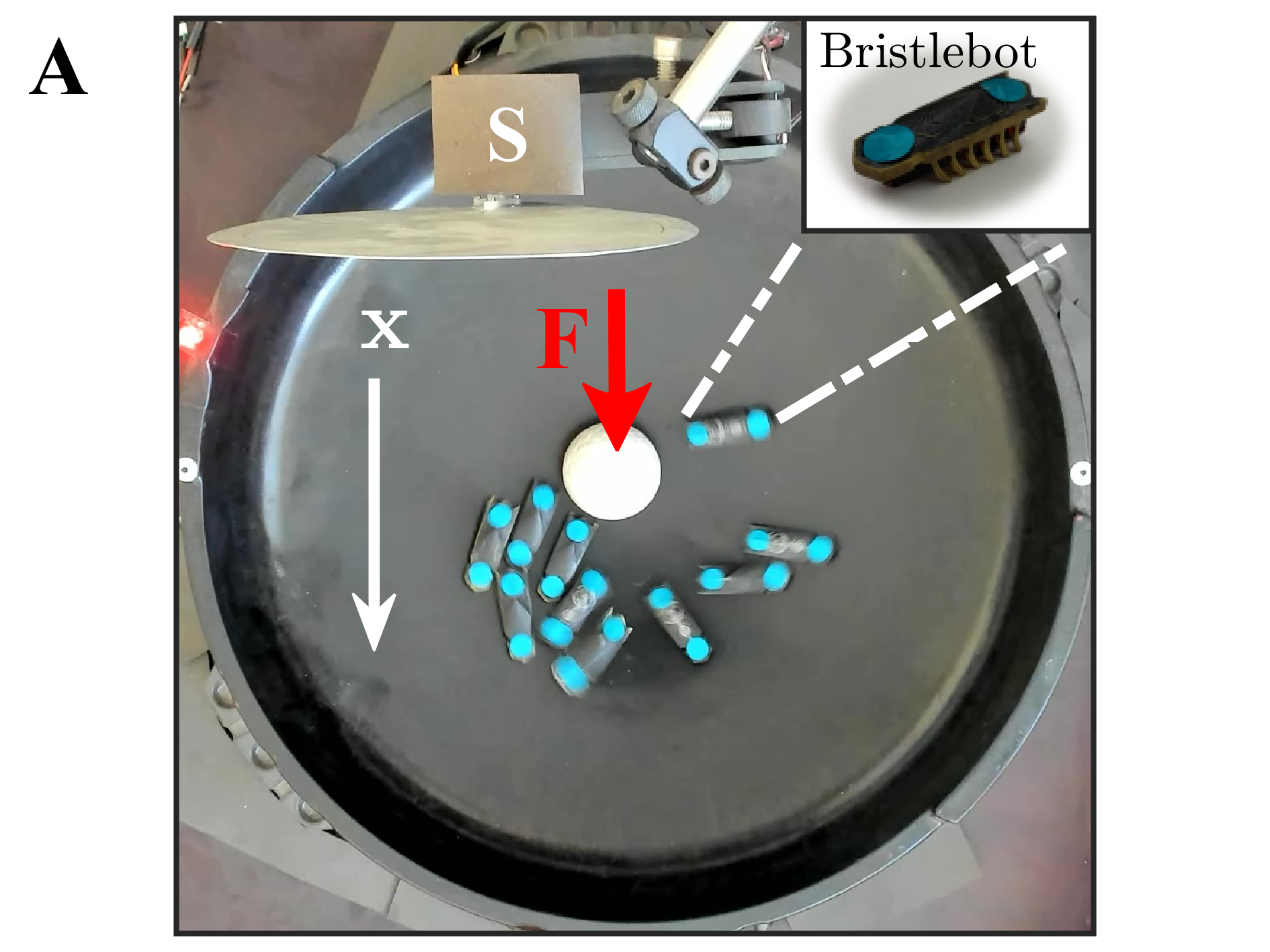
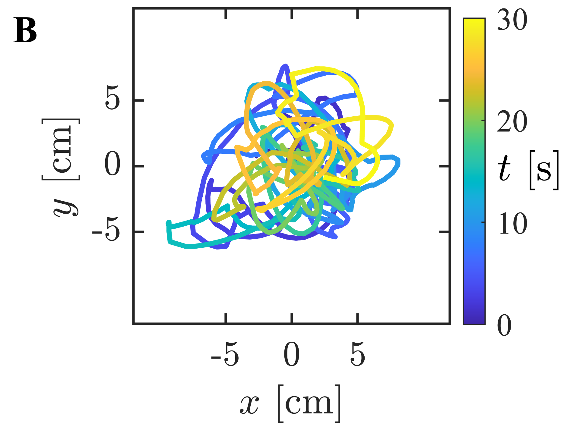
Figure 1: Experimental setup.  A.  A Styrofoam ball (diameter $\sim 4$ cm) is trapped in a gravitational harmonic potential, a plastic bowl (diameter 38cm, depth 5cm), and subjected to collisions with self-propelled bbots (inset: standard bot, $4\times 1$ cm). The ball is repeatedly perturbed with a uniform air stream created by an external fan along the $x$-axis (white arrow) to test a fluctuation-response relation. To enforce an abrupt onset and release of the perturbation, a mechanical shutter is used (denoted by ’S’). B.  Part ($30$ s) of a typical trajectory of the Styrofoam ball in a $N_{b}=10$ bbots arena (see also SM movie 1).

Our experiments are conducted as depicted in Fig. 1A: a Styrofoam ball is placed in a parabolic plastic arena and is driven into a nonequilibrium steady state by random collisions with an assembly of vibration-driven bristle robots (bbots, Hexbugs${}^{\text{TM}}$ nano, [48, 49, 17, 50, 51]). The motion of the ball is recorded by a top-view camera (Brio 4K, Logitech) at $30~{}\text{fps}$. An image analysis algorithm is then used to extract the trajectory of the ball (Fig. 1B). The collisions between the bbots in the arena, and their collisions with the ball, randomize their propulsion direction, resulting in an active gas-like state (see SM movie 1). We note that in contrast to shaken granular matter, the embedding media is active on the single particle level and exhibits emergent collective motion typical for active matter systems [48].

To measure the system’s mean response, we introduce a mechanical perturbation by activating an external fan (Yate Loon electronics $12$ V $0.30$ A cooling fan) to create an airflow. After the tracer settles into a perturbed steady state, we abruptly deactivate the disturbance, with a physical shutter, allowing the ball to return to its original steady state.

We use the number of bbots $N_{b}$ as a control parameter, keeping the trapping stiffness constant, i.e., the arena shape and tracer size are held constant. Naturally, the mean free time between collisions $\tau_{c}$ decreases with $N_{b}$, and the collision frequency increases (see below).

Since thermal forces are negligible, the ensemble of bbots $N_{b}$ acts as a dry active bath, meaning that the tracer is subjected to a single active noise source. Therefore, the noise characteristic time $\tau_{c}$ and the stationary relaxation time $\tau_{r}$ are intrinsic system timescales. Particularly, collisions between the bbots and the Styrofoam ball are the main source of deceleration as they are the main source of acceleration. Hence, the main channel for dissipation is the same process that induces active fluctuations, and we expect a generalized FDR to hold for the wide range of $N_{b}$ used here, as was suggested by Kubo for equilibrium conditions [2].

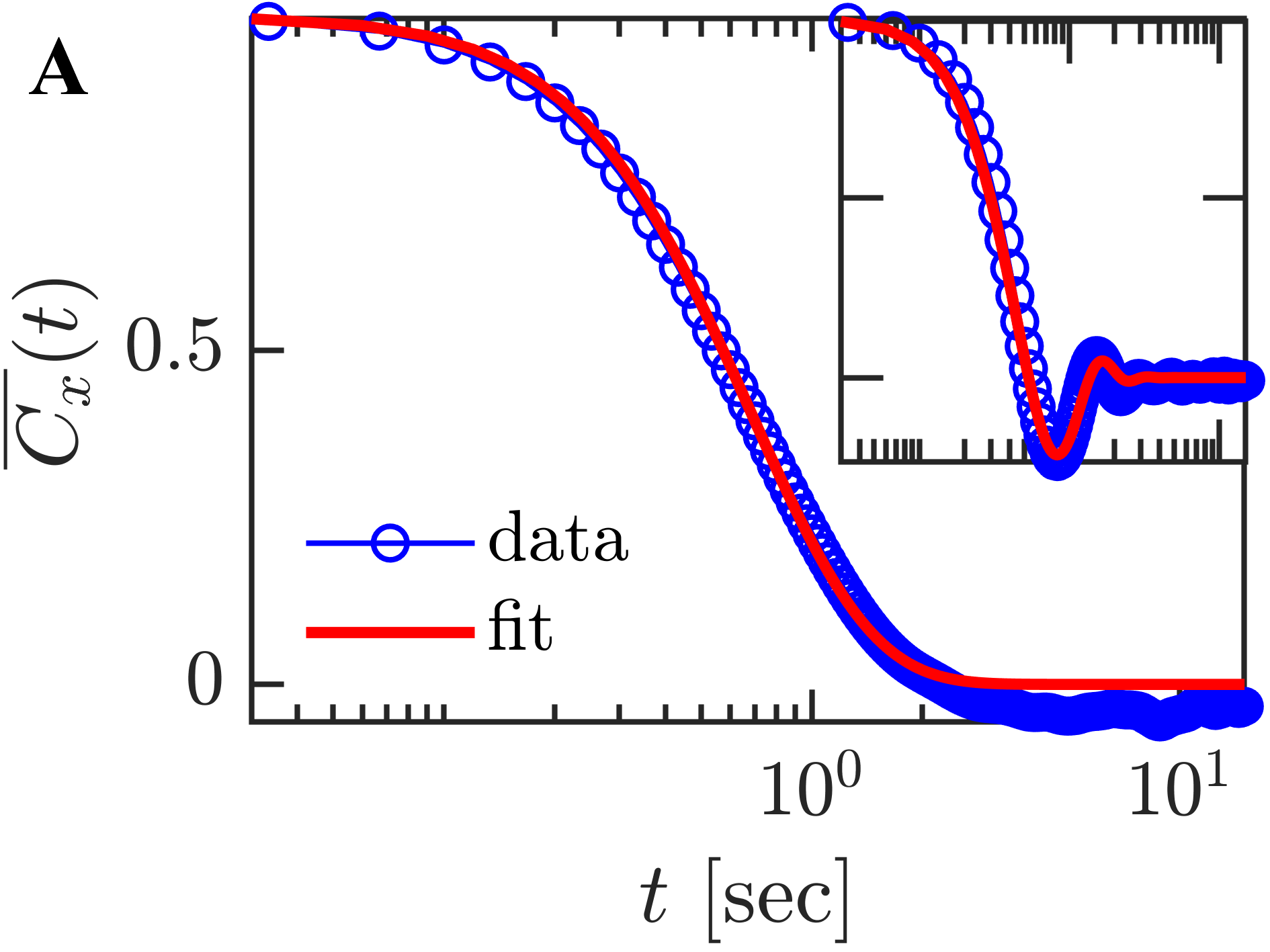
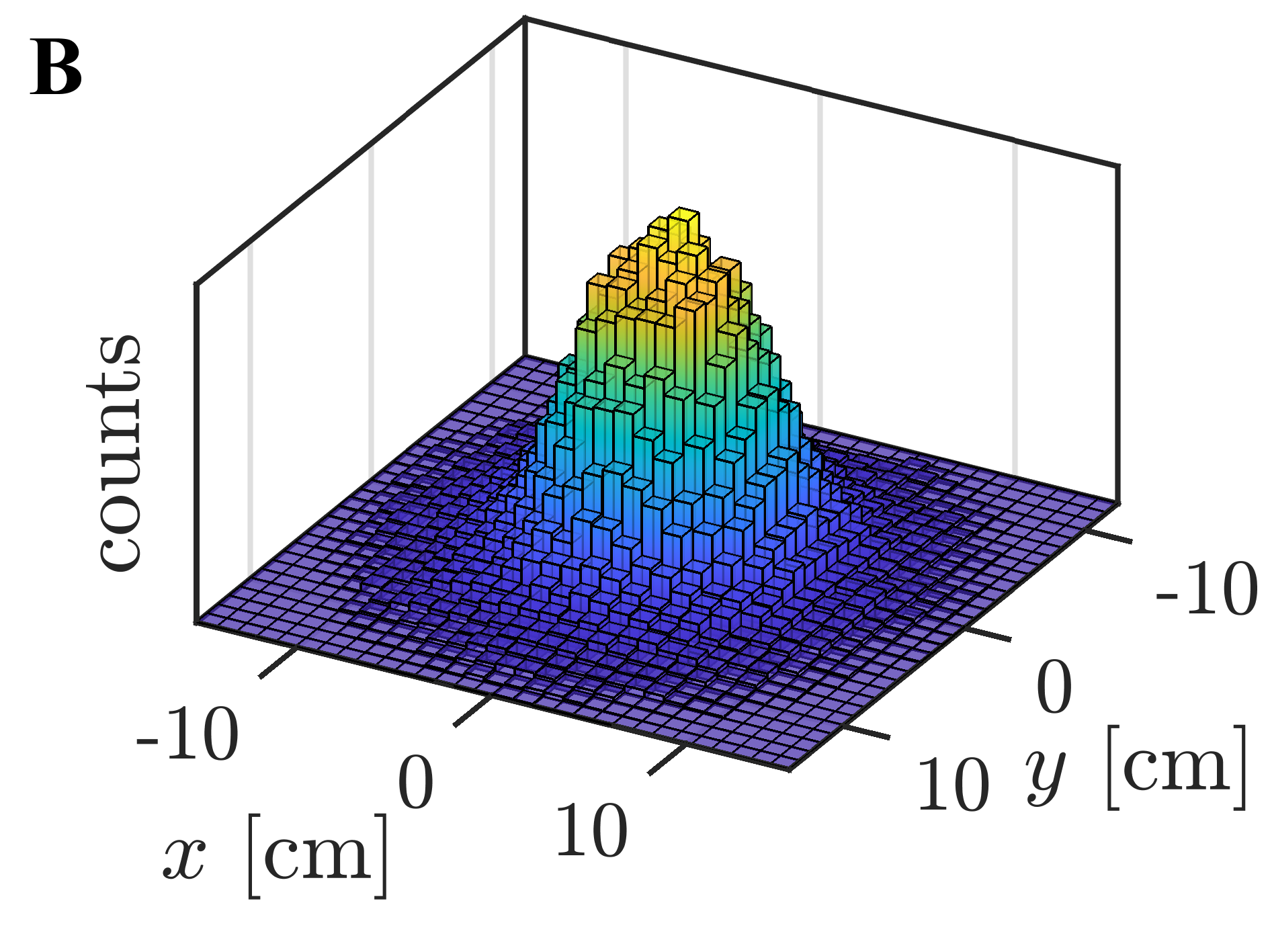
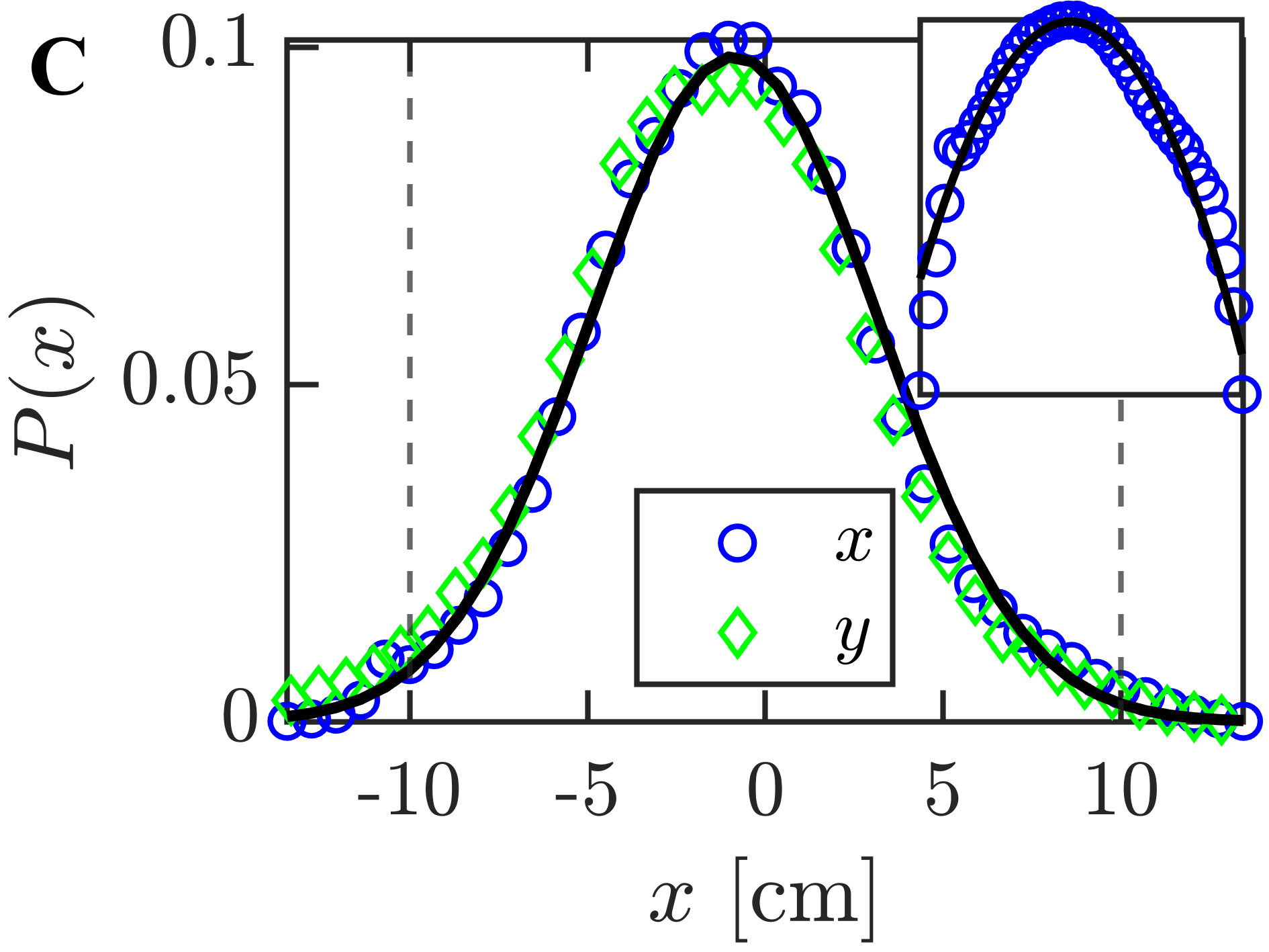
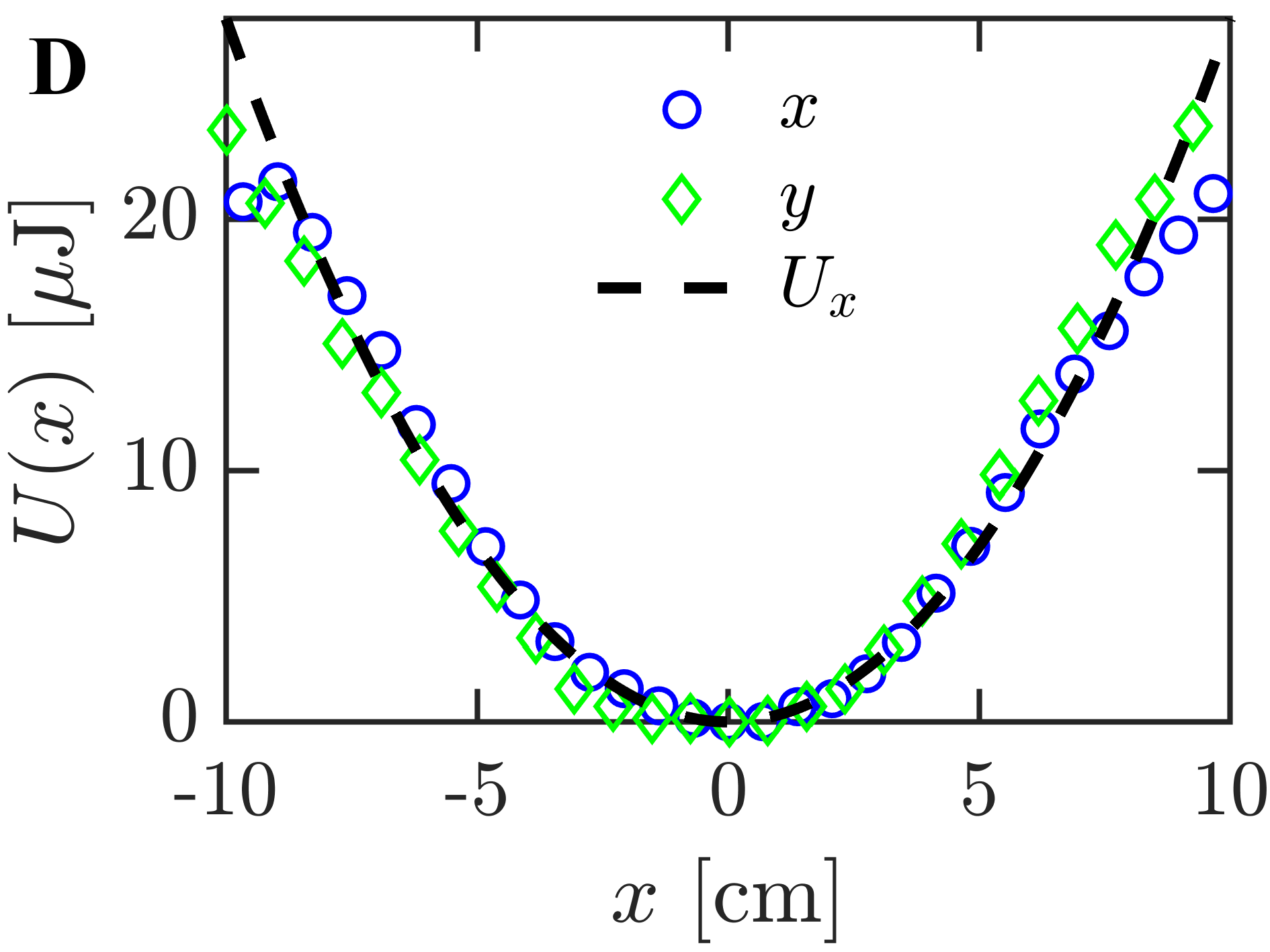
Figure 2: Stationary position dynamics and statistics. A.  Normalized measured position autocorrelation function as a function of time (circles) for $N_{b}=15$, and fit to Eq. 2, with $\tau_{r}=0.336\approx\tau_{\Omega}=0.340$ s (solid line). The inset shows the autocorrelation of an equivalent experiment with $N_{b}=4$ ($\tau_{r}=0.54$ s, $\tau_{\Omega}=0.23$ s) B.  A 3D ($x,y$) tracer position histogram. C.  The cross-section probability density distributions across the $x$ axis (blue), and the $y$ axis (green). The solid line is a fit to a Normal distribution. The dashed lines ($|x|=10$ cm) mark the boundaries of the harmonic part of the trap. D.  The physical trapping potential $U_{x}(x)=mgax^{2}$ (dashed line), compared to the Boltzmann statistics based experimental estimate of the potential. The results are obtained by averaging $M=375$ tracer position time-sequences, with $t\in[0,30]$ s, in a $N_{b}=15$ bbot bath.

Stationary dynamics and statistics.– We start our experiments by characterizing the nonequilibrium steady state, which we will later perturb. To this end, we focus on a system with a relatively large number of bbots, $N_{b}=15$, in which the tracer particle is subjected to frequent collisions with $\tau_{c}=0.28$ s, extracted by image analysis identification of collisions. We record 375 experiments of duration $30$ s from which the tracer particle trajectory is extracted. From the extracted trajectories, we calculate the tracer’s (ensemble) average normalized position autocorrelation, $\overline{C_{x}}(t)$ (Fig. 2A). It turns out that this correlation is well fit by the generic autocorrelated function of damped noisy harmonic oscillator [28, 18, 45],

$$\overline{C_{x}}(t)\equiv\frac{C_{x}(t)}{\langle\Delta x^{2}\rangle_{0}}=e^{-t/\tau_{r}}\left(\cos\omega t+\frac{\sin\omega t}{\tau_{r}\omega}\right),$$ (2)

where $\langle\Delta x^{2}\rangle_{0}=C_{x}(0)$ is the variance and $\omega^{2}=\tau_{\Omega}^{-2}-\tau_{r}^{-2}$. This fit provides effective values of the system’s time scale, the damping rate, $2\tau_{r}^{-1}$, and the natural frequency of the bbot harmonic trap, $\tau_{\Omega}^{-1}$, , for which we obtain $\tau_{r}=0.336\approx\tau_{\Omega}=0.340$ s. These values suggest that the tracer dynamics exhibit critically damped behavior. We note that underdamped relaxation ($\tau_{r}>\tau_{\Omega}$) is observed for much lower $N_{b}=4$ (inset of Fig. 2A).

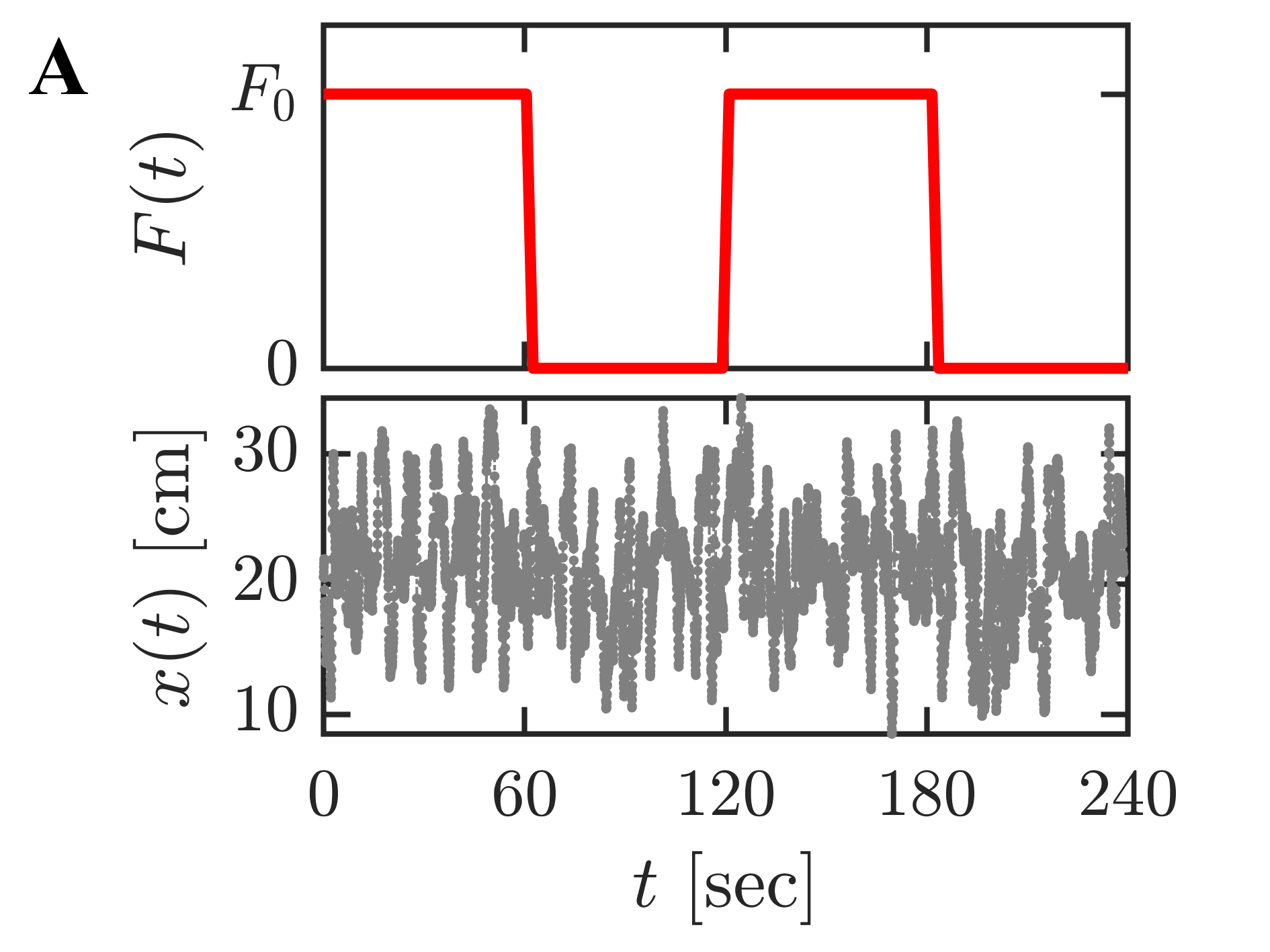
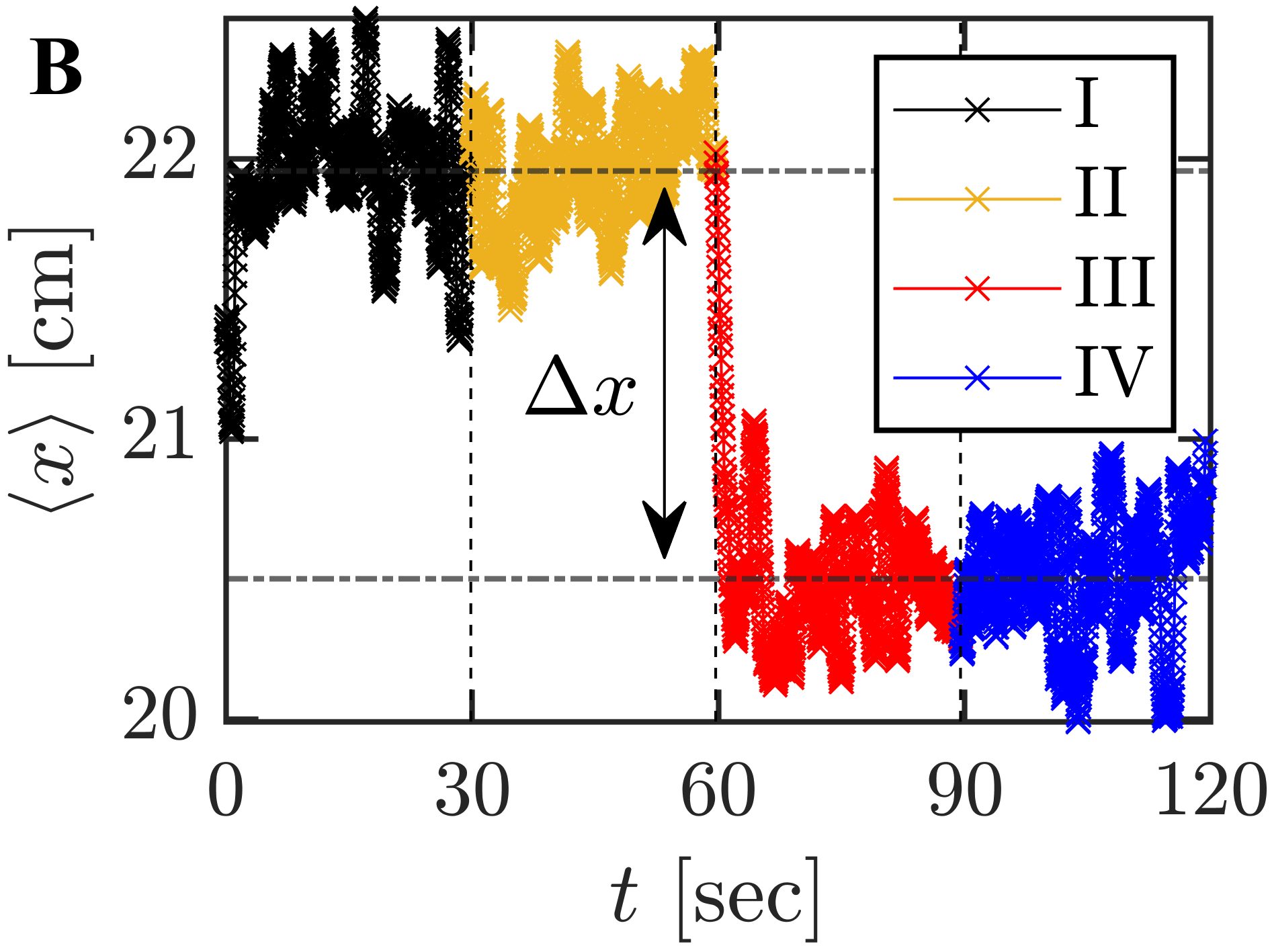
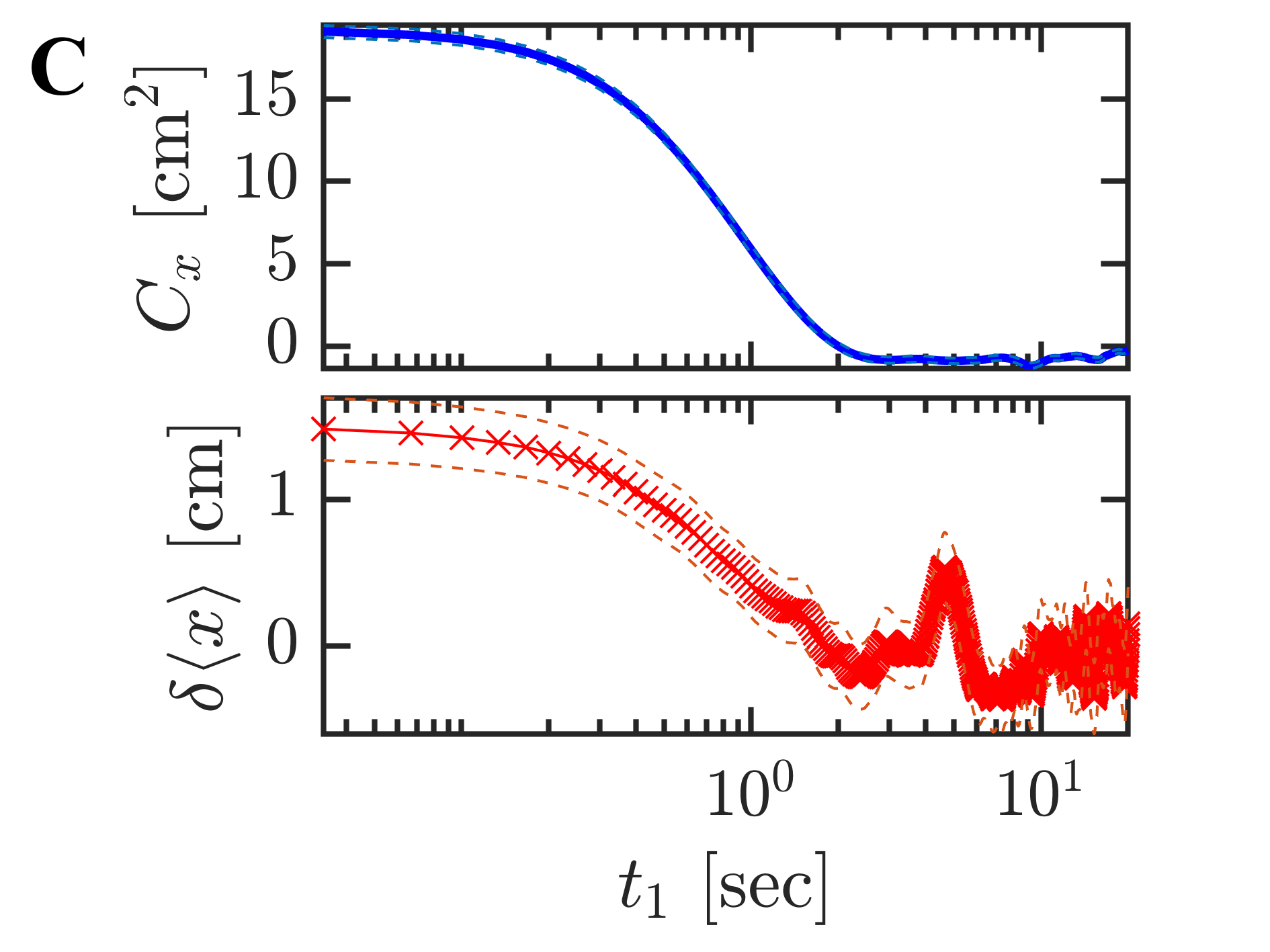
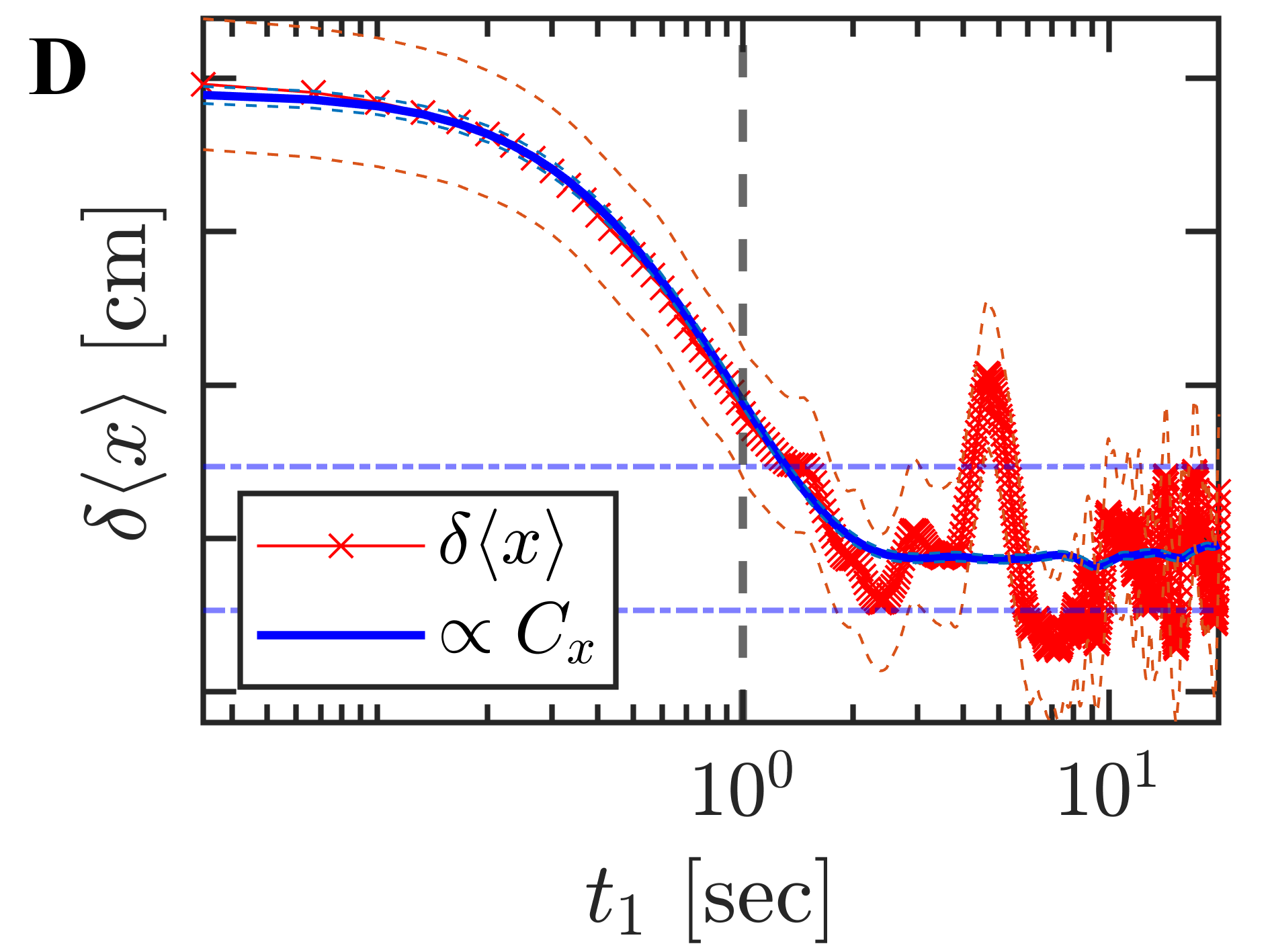
Figure 3: An experimental FDR test. A.  A typical perturbation sequence $x(t)$: the fan is turned on for a minute and then abruptly turned off for the following minute. B.  The time-dependent mean value $\langle x(t)\rangle$ is obtain within a time-window of $2$ minutes. The latter is split into four parts to extract both response and correlation properties conveniently. Namely, part I is discarded, part II is the perturbed steady state, part III is the response to the force switch-off, and part IV is the unperturbed steady state. The displacement $\Delta x$ is the mean distance between states II and IV. C.  The individual time-dependent quantities of transient response $\langle x(t_{1})\rangle-\langle x\rangle_{0}$ (bottom), and unperturbed autocorrelation function $C_{x}(t_{1})$ (top), are displayed. The dashed lines are standard errors. D.  The generalized FDR of Eq. 1 with an effective temperature $T=T_{\text{eff}}\sim\langle\Delta x^{2}\rangle_{0}$, is validated. The results present an average over $M=375$ sequences with $N_{b}=15$. The vertical dashed line is $T_{c}=1$ s and the horizontal dot-dashed lines (blue) are the standard errors of the steady state of part IV.

Next, we consider the position probability distribution $P(x,y)$, of the tracer particle (Fig. 2B). We find that $P(x,y)$ fits well to a Boltzmann-like Gaussian distribution in both $x$ and $y$ projections (Fig. 2C), with a small expected deviation near the arena boundaries ($|x|>10$ cm). We estimate the gravitational potential acting on the tracer particle by $U_{x}(x)=\frac{1}{2}kx^{2}$, with $k=mga=2.8\pm 0.3~{}\text{g/s}^{-2}$, $m=1\pm 0.1$ g - the tracer mass, $g$ - the gravitational acceleration, and $a$ - the curvature of the arena. Plotting the estimated $U_{x}(x)$ and fitting it to our Boltzmann-like position distribution, we obtain an effective temperature of $T_{\text{eff}}\approx 3.1\cdot 10^{17}$ K, 15 orders of magnitude higher than room temperature (Fig. 2D).

Fluctuation-dissipation relations.– With a full characterization of the nonequilibrium steady state dynamics and statistics of the system, we continue by measuring the system’s response to a small mechanical perturbation (force $F_{0}\approx 6.2~{}\mu\text{N}$). We use the following protocol to measure the ensemble average response of the system (see also Ref. [17] for a similar procedure): during an experiment, every two minutes, the fan is turned on for a minute and abruptly turned off at $t_{0}=60$ s for the following minute (see Fig. 3A). Fig. 3B shows the time-dependent mean value $\langle x(t)\rangle$ for $M=375$ perturbation sequences, constituting both the mean motion of the tracer at the perturbed and unperturbed steady states (parts II and IV) and the transition between them (parts I and III).

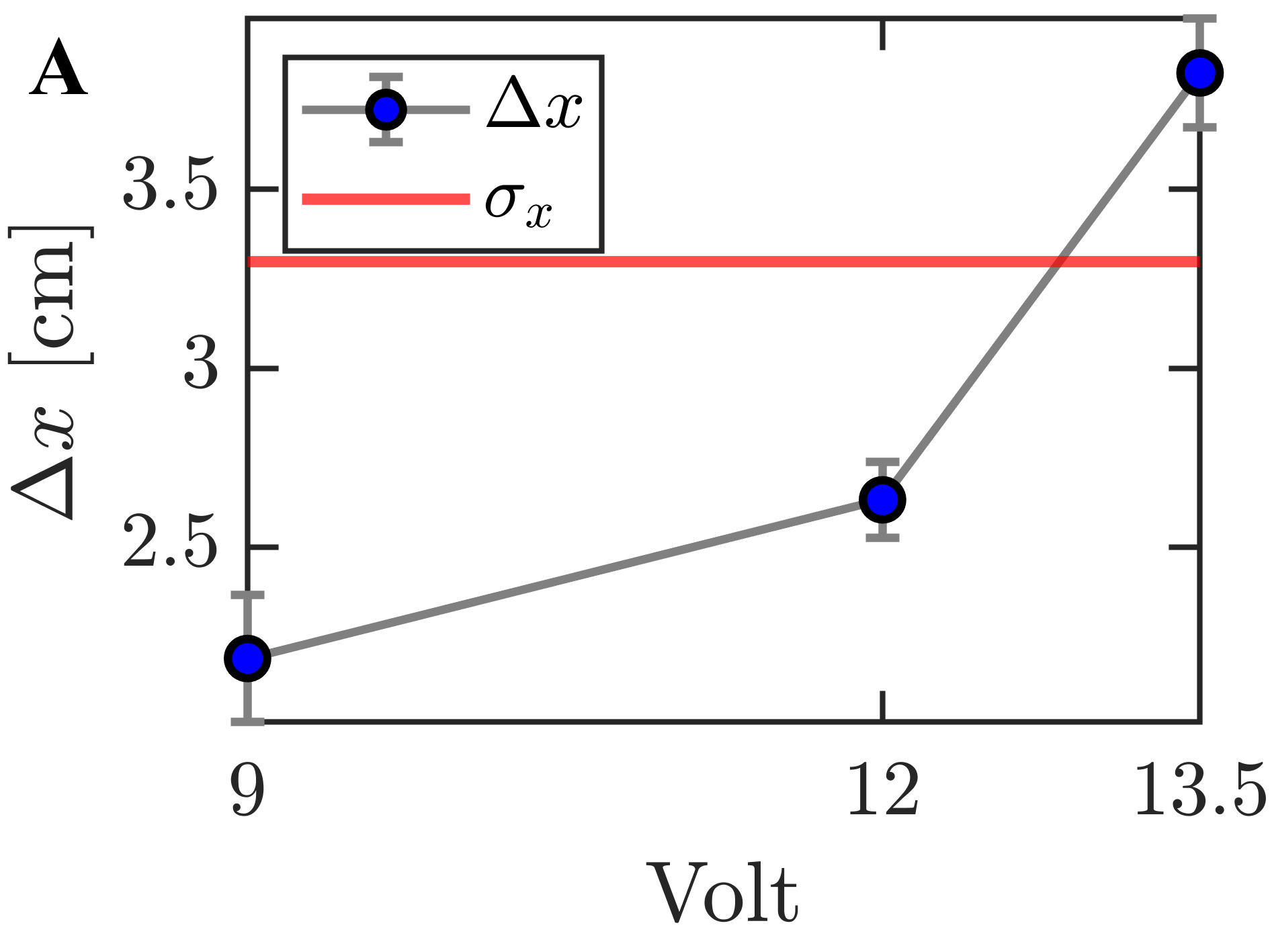
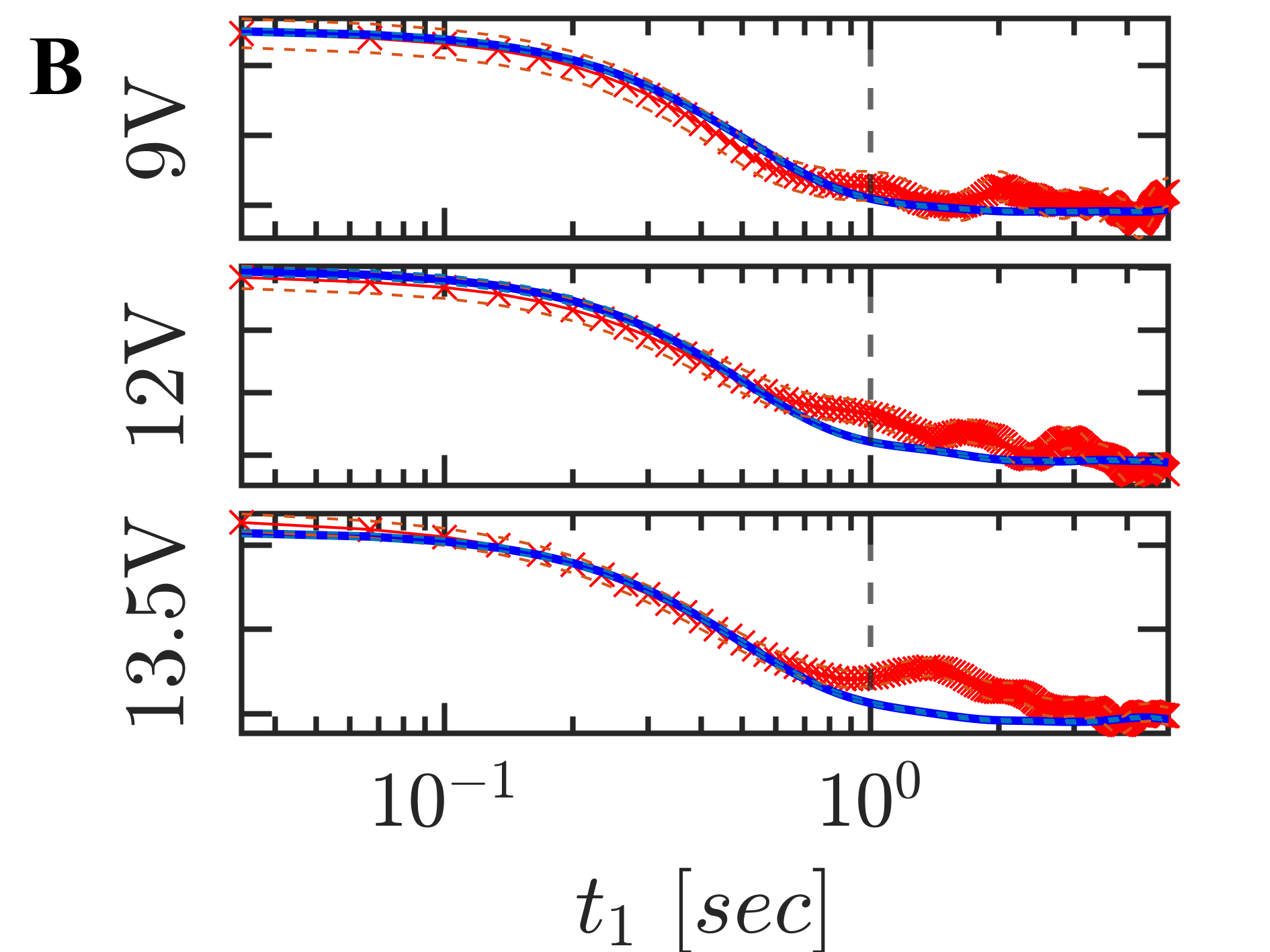
Figure 4: The dynamic FDR under different perturbation amplitudes. A.  The mean displacement $\Delta x$, under a perturbation as a function of fan voltage (the error bars are the standard errors). The applied force $F_{0}=k\Delta x$ increases with $V$. The tracer’s position standard deviation, $\sigma_{x}$, is used to define the range of small perturbations (solid line). B.  the corresponding generalized FDRs with $T_{\text{eff}}\sim\langle\Delta x^{2}\rangle_{0}$ are plotted for $V=9,\ 12,\ 13.5$ V. The results present an average over $M=375$ sequences with $N_{b}=10$.

The response of the system to the perturbation arrest, at ${t_{1}}=t-t_{0}$, given by $R_{x}(t_{1})=\delta\langle x(t_{1})\rangle=\langle x(t_{1})\rangle-\langle x\rangle_{0}$, and the unperturbed autocorrelation function, $C_{x}(t_{1})=\langle x(t_{1})x(0)\rangle_{0}$, are therefore measured from parts III, and IV respectively (Fig. 3C). According to the generalized FDR, Eq. 1 should hold exactly for our measured response and autocorrelation if we define $T=T_{\text{eff}}$ and $F_{0}=k\Delta x$, where $\Delta x\equiv\langle x\rangle_{F_{0}}-\langle x\rangle_{0}$. This is verified in Fig. 3D with good accuracy, where we have used the value of $T_{\text{eff}}$ obtained from the stationary position distribution. We note that at $t_{1}>T_{c}=1$ s the stationary noise becomes significant and the agreement or disagreement of $C_{x}$ and $R_{x}$ is hard to assess. Therefore, we cannot rule out an FDR violation beyond $T_{c}$.

Since $T_{\text{eff}}$ fulfills the generalized FDR for any $t_{1}<T_{c}$, it also fulfills it at $t_{1}=0$. Therefore, $k_{B}T_{\text{eff}}=k\langle\Delta x^{2}\rangle_{0}$, which is trivial for a system exhibiting Boltzmann-like statistics. However, this relation should generally hold for any $P(x,y)$ (with different $N_{b}$).

We test the validity of the generalized FDR further by varying the perturbation amplitude (fan voltage) at constant $N_{b}$ and $T_{\text{eff}}$. Figure 4A shows an increase in the measured mean displacements $\Delta x$ as a function of the fan operating voltage. We find that when $\Delta x>\sigma_{x}$ for $V=13.5$ V (Fig. 4A), we are beyond the linear response regime. Consequently, in Fig. 4B we observe that deviations from a generalized FDR become notably more pronounced under stronger perturbations.

Our experimental findings establish a consistent effective temperature, $T_{\text{eff}}$, derived from the generalized fluctuation-dissipation relation (FDR). This $T_{\text{eff}}$ is consistent with the temperature determined by the average potential energy and remains independent of the force. With this defined $T_{\text{eff}}$, we can further explore the conditions under which the generalized FDR remains applicable.

Range of validity of the FDR.– Finally, we repeat our experiments for different numbers of bbots in the arena, $4<N_{b}<17$. In Fig. 5A (upper panel) the displayed characteristic times exhibit a dependence on the system configuration $N_{b}$, i.e., the evaluated mean free time between collisions $\tau_{c}$ and the Langevin typical times $\tau_{r}$, $\tau_{\Omega}$ (fit to Eq. 2). We observe that $\tau_{r}$ and $\tau_{c}$ decrease with $N_{b}$, as the dynamics become less oscillatory, approaching a critically-damped behavior at $N_{b}=15,~{}\text{and}~{}17$. By using a consistent definition of effective temperature for all configurations, $T_{\text{eff}}=k\langle\Delta x^{2}\rangle_{0}$, we observe a monotonic increase in $T_{\text{eff}}$ with $N_{b}$ (Fig. 5A, middle panel). We quantify the departure from Boltzmann statistics by calculating the non-Gaussian parameter of the position distribution, $\Gamma=\frac{\langle x^{4}\rangle}{3\langle x^{2}\rangle^{2}}-1$ (see Fig. 5A, lower panel), and find that $P(x,N_{b})$ transitions into a non-Gaussian distribution as $N_{b}$ decreases (Fig. 5B).

The generalized FDRs for different $N_{b}$ are displayed in Fig. 5C and are empirically satisfied within the response time regime. We, therefore, find that a generalized FDR, with an effective temperature as defined here, is generally valid for all our experiments regardless of the functional form of the stationary position distribution, both for underdamped and critically-damped dynamics.

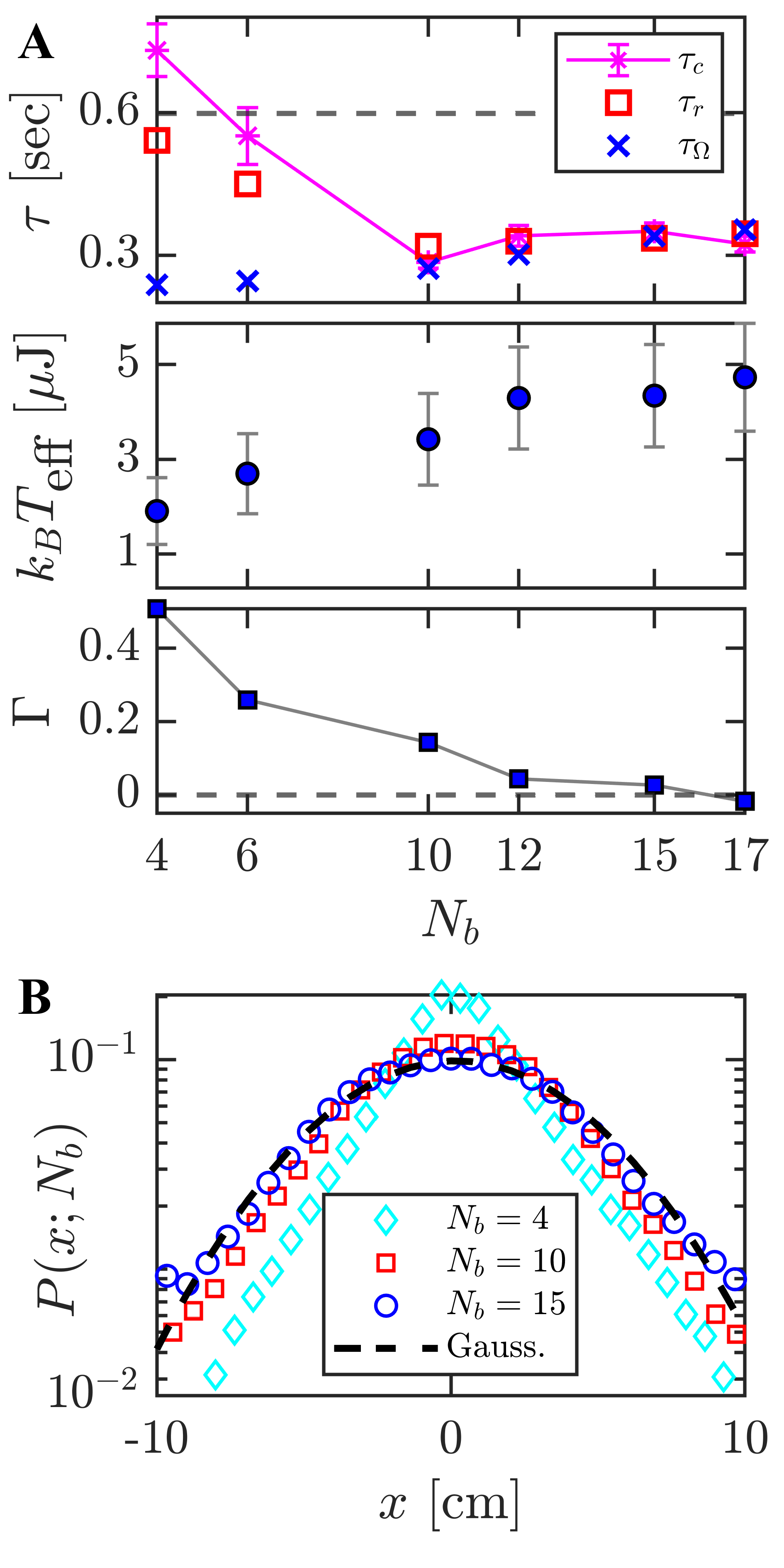
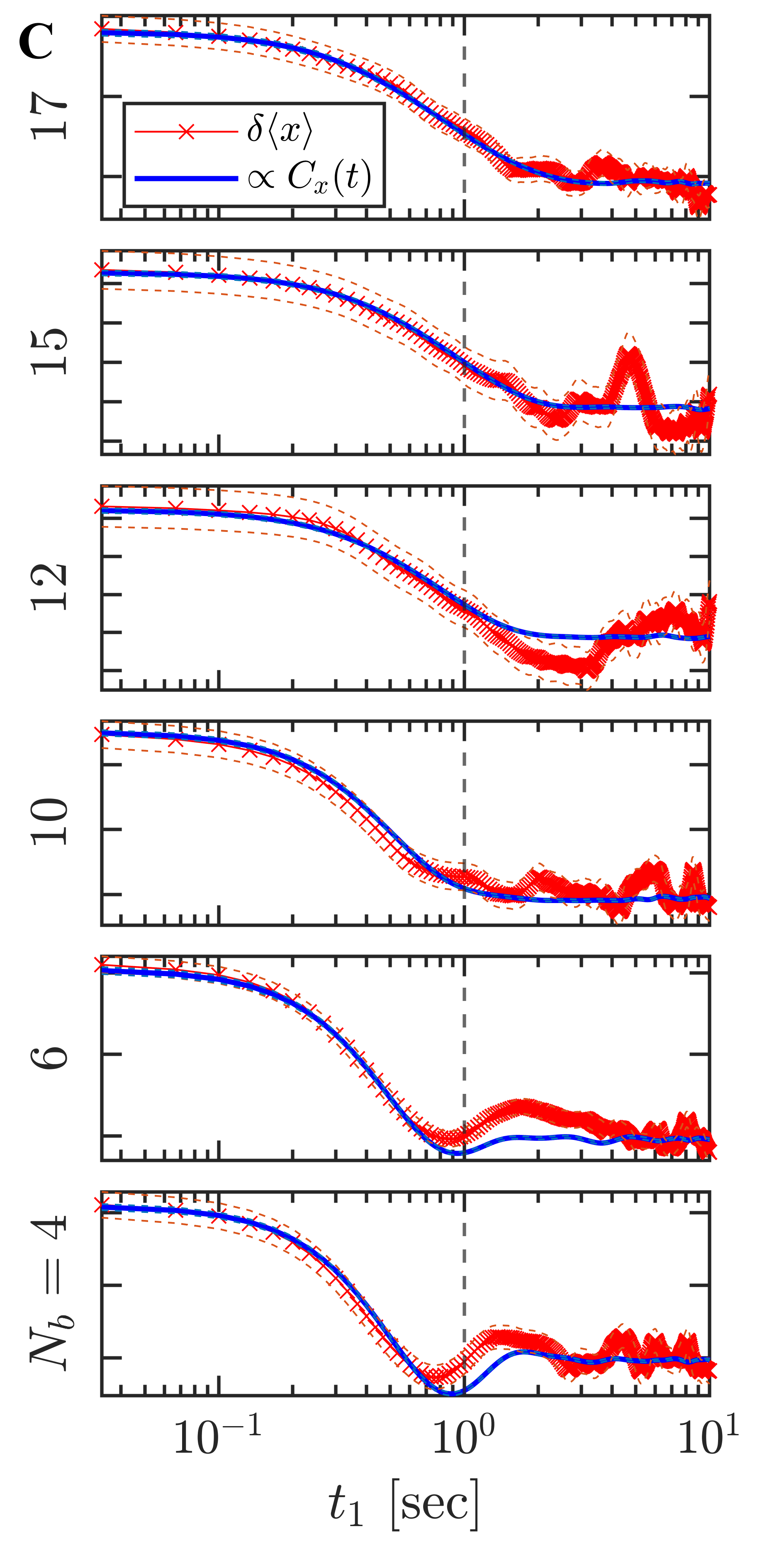
Figure 5: Effective temperatures and FDRs of different bbot configurations. We consider configurations of $N_{b}=\{4,6,10,12,15,17\}$ bbot baths. The results were obtained for an ensemble average of $M=375$ perturbation sequences, with the same tracer $m\approx 1$ g, gravitational stiffness $k\approx 2.8~{}\text{g/s}^{-2}$, and fan operating voltage with $\Delta x(V)<\sigma_{x}$. A.  Different metastatistics vs. number of bbots. Top panel: mean free time between collisions $\tau_{c}$ (magenta, line), Langevin timescales (obtained by a fit to Eq. 2) $\tau_{r}$ (red, squares) and $\tau_{\Omega}$ (blue, crosses), and oscillation period in the potential $\sqrt{m/k}$ (dashed line) Middle panel: effective temperature $T_{\text{eff}}$ (circles, middle panel). Lower panel: non-Gaussian parameter (squares), $\Gamma=\langle x^{4}\rangle/3\langle x^{2}\rangle^{2}-1$. Error-bars are standard deviations. B.  Position probability density for $N_{b}=4$ (diamonds), $10$ (squares), $15$ (circles). Dashed line is the normal (Gaussian) distribution for $N_{b}=15$. C.  Corresponding generalized FDRs (Eq. 1 with $T=T_{\text{eff}}$) for all configurations $N_{b}$. The vertical dashed lines are $T_{c}=1$ s.

Discussion.– In summary, we have experimentally confirmed the validity of a generalized FDR, far from equilibrium, in a large range of conditions. Here, the transient response to a perturbation and the stationary correlations are characterized by a time-dependent relaxation towards a steady state. These quantities exhibit equilibrium-like proportionality via $T_{\text{eff}}$, with dynamics that become less oscillatory as $N_{b}$ rises. The similar values of the evaluated $\tau_{r}$ and $\tau_{c}$, indicate that the number of bath particles $N_{b}$ governs both the damping rate and the effective temperature ($T_{\text{eff}}\sim\langle\Delta x^{2}\rangle_{0}$) of the tracer. In essence, the bots play a central role in both energy dissipation and fluctuation generation in the system.

We focused on experimental setups with $4<N_{b}<17$ for two main reasons. When $N_{b}<4$, the tracer is rarely perturbed, and conversely, when $N_{b}>17$, finite system size leads to large clusters at the trap’s center. It is noteworthy that although possible violations are observed at increasingly lower times as $N_{b}$ decreases, and the analogy to a heat bath becomes limited, the dynamic FDR with $T_{\text{eff}}\sim\langle\Delta x^{2}\rangle_{0}$ holds, within statistical accuracy ($t_{1}<T_{c}$), even at $N_{b}<12$ when the tracer’s position distribution is highly non-Gaussian.

The confirmation of a generalized FDR, across an extensive range of effective temperatures, raises the following three broader issues. Is there an overarching equipartition relation that connects these effective temperatures to $T_{\text{eff}}$ defined via momentum variables rather than positional ones?

Secondly, do these temperatures hold significance within the thermodynamic framework governing these systems? For instance, could they dictate energy flow in scenarios where two such systems are in contact?

Lastly, our experimental observations reveal that our tracer dynamics exhibit consistency with Markovian dynamics [17]. While Markovianity is not essential for the FDR to prevail in thermal equilibrium, an intriguing avenue of exploration involves assessing its validity in weakly perturbed systems immersed in an active, non-Markovian environment, where dissipation and fluctuation derive from the same underlying physical process.

References

- Einstein [1905] A. Einstein, On the motion of small particles suspended in liquids at rest required by the molecular-kinetic theory of heat, Ann. Phys. (Leipzig) 17, 208 (1905).
- Kubo [1966] R. Kubo, The fluctuation-dissipation theorem, Rep. Prog. Phys. 29, 255 (1966).
- Kubo [1986] R. Kubo, Brownian motion and nonequilibrium statistical mechanics, Science 233, 330 (1986).
- Marconi et al. [2008] U. M. B. Marconi, A. Puglisi, L. Rondoni, and A. Vulpiani, Fluctuation-dissipation: response theory in statistical physics, Phys. Rep. 461, 111 (2008).
- Baldovin et al. [2022] M. Baldovin, L. Caprini, A. Puglisi, A. Sarracino, and A. Vulpiani, The many faces of fluctuation-dissipation relations out of equilibrium (Springer, 2022) pp. 29–57.
- Martin et al. [2001] P. Martin, A. Hudspeth, and F. Jülicher, Comparison of a hair bundle’s spontaneous oscillations with its response to mechanical stimulation reveals the underlying active process, Proc. Natl. Acad. Sci. 98, 14380 (2001).
- Mizuno et al. [2007] D. Mizuno, C. Tardin, C. F. Schmidt, and F. C. MacKintosh, Nonequilibrium mechanics of active cytoskeletal networks, Science 315, 370 (2007).
- Turlier et al. [2016] H. Turlier, D. A. Fedosov, B. Audoly, T. Auth, N. S. Gov, C. Sykes, J.-F. Joanny, G. Gompper, and T. Betz, Equilibrium physics breakdown reveals the active nature of red blood cell flickering, Nat. Phys. 12, 513 (2016).
- Prost et al. [2009] J. Prost, J.-F. Joanny, and J. M. Parrondo, Generalized fluctuation-dissipation theorem for steady-state systems, Phys. Rev. Lett. 103, 090601 (2009).
- Mehl et al. [2010] J. Mehl, V. Blickle, U. Seifert, and C. Bechinger, Experimental accessibility of generalized fluctuation-dissipation relations for nonequilibrium steady states, Phys. Rev. E 82, 032401 (2010).
- Dybiec et al. [2012] B. Dybiec, J. M. Parrondo, and E. Gudowska-Nowak, Fluctuation-dissipation relations under Lévy noises, Europhys. Lett. 98, 50006 (2012).
- Willareth et al. [2017] L. Willareth, I. M. Sokolov, Y. Roichman, and B. Lindner, Generalized fluctuation-dissipation theorem as a test of the Markovianity of a system, Europhys. Lett. 118, 20001 (2017).
- Lindner [2022] B. Lindner, Fluctuation-dissipation relations for spiking neurons, Phys. Rev. Lett. 129, 198101 (2022).
- Pérez-Cervera et al. [2023] A. Pérez-Cervera, B. Gutkin, P. J. Thomas, and B. Lindner, A universal description of stochastic oscillators, PNAS 120, e2303222120 (2023).
- Lippiello et al. [2008] E. Lippiello, F. Corberi, A. Sarracino, and M. Zannetti, Nonlinear response and fluctuation-dissipation relations, Phys. Rev. E 78, 041120 (2008).
- Lucarini and Colangeli [2012] V. Lucarini and M. Colangeli, Beyond the linear fluctuation-dissipation theorem: the role of causality, J. Stat. Mech. 2012, P05013 (2012).
- Engbring et al. [2023] K. Engbring, D. Boriskovsky, Y. Roichman, and B. Lindner, A nonlinear fluctuation-dissipation test for Markovian systems, Phys. Rev. X 13, 021034 (2023).
- Ojha et al. [2004] R. Ojha, P.-A. Lemieux, P. Dixon, A. Liu, and D. Durian, Statistical mechanics of a gas-fluidized particle, Nature 427, 521 (2004).
- Villamaina et al. [2008] D. Villamaina, A. Puglisi, and A. Vulpiani, The fluctuation-dissipation relation in sub-diffusive systems: the case of granular single-file diffusion, J. Stat. Mech. 2008, L10001 (2008).
- Maggi et al. [2014] C. Maggi, M. Paoluzzi, N. Pellicciotta, A. Lepore, L. Angelani, and R. Di Leonardo, Generalized energy equipartition in harmonic oscillators driven by active baths, Phys. Rev. Lett. 113, 238303 (2014).
- Szamel [2014] G. Szamel, Self-propelled particle in an external potential: Existence of an effective temperature, Phys. Rev. E 90, 012111 (2014).
- Dieterich et al. [2015] E. Dieterich, J. Camunas-Soler, M. Ribezzi-Crivellari, U. Seifert, and F. Ritort, Single-molecule measurement of the effective temperature in non-equilibrium steady states, Nat. Phys. 11, 971 (2015).
- Maggi et al. [2017] C. Maggi, M. Paoluzzi, L. Angelani, and R. Di Leonardo, Memory-less response and violation of the fluctuation-dissipation theorem in colloids suspended in an active bath, Sci. Rep. 7, 17588 (2017).
- Petrelli et al. [2020] I. Petrelli, L. F. Cugliandolo, G. Gonnella, and A. Suma, Effective temperatures in inhomogeneous passive and active bidimensional Brownian particle systems, Phys. Rev. E 102, 012609 (2020).
- Flenner and Szamel [2020] E. Flenner and G. Szamel, Active matter: Quantifying the departure from equilibrium, Phys. Rev. E 102, 022607 (2020).
- Solon and Horowitz [2022] A. Solon and J. M. Horowitz, On the Einstein relation between mobility and diffusion coefficient in an active bath, J. Phys. A 55, 184002 (2022).
- Boudet et al. [2022] J. F. Boudet, J. Jagielka, T. Guerin, T. Barois, F. Pistolesi, and H. Kellay, Effective temperature and dissipation of a gas of active particles probed by the vibrations of a flexible membrane, Phys. Rev. Res. 4, L042006 (2022).
- Uhlenbeck and Ornstein [1930] G. E. Uhlenbeck and L. S. Ornstein, On the theory of the Brownian motion, Phys. Rev. 36, 823 (1930).
- Bechinger et al. [2016] C. Bechinger, R. Di Leonardo, H. Löwen, C. Reichhardt, G. Volpe, and G. Volpe, Active particles in complex and crowded environments, Rev. Mod. Phys. 88, 045006 (2016).
- Fodor et al. [2016] É. Fodor, C. Nardini, M. E. Cates, J. Tailleur, P. Visco, and F. Van Wijland, How far from equilibrium is active matter?, Phys. Rev. Lett. 117, 038103 (2016).
- Démery and Fodor [2019] V. Démery and É. Fodor, Driven probe under harmonic confinement in a colloidal bath, J. Stat. Mech. 2019, 033202 (2019).
- Ye et al. [2020] S. Ye, P. Liu, F. Ye, K. Chen, and M. Yang, Active noise experienced by a passive particle trapped in an active bath, Soft Matter 16, 4655 (2020).
- Martin et al. [2021] D. Martin, J. O’Byrne, M. E. Cates, É. Fodor, C. Nardini, J. Tailleur, and F. Van Wijland, Statistical mechanics of active Ornstein-Uhlenbeck particles, Phys. Rev. E 103, 032607 (2021).
- Shea et al. [2022] J. Shea, G. Jung, and F. Schmid, Passive probe particle in an active bath: can we tell it is out of equilibrium?, Soft Matter 18, 6965 (2022).
- Wu and Libchaber [2000] X.-L. Wu and A. Libchaber, Particle diffusion in a quasi-two-dimensional bacterial bath, Phys. Rev. Lett. 84, 3017 (2000).
- Chen et al. [2007] D. T. Chen, A. Lau, L. A. Hough, M. F. Islam, M. Goulian, T. C. Lubensky, and A. G. Yodh, Fluctuations and rheology in active bacterial suspensions, Phys. Rev. Lett. 99, 148302 (2007).
- Angelani et al. [2009] L. Angelani, R. Di Leonardo, and G. Ruocco, Self-starting micromotors in a bacterial bath, Phys. Rev. Lett. 102, 048104 (2009).
- Cisneros et al. [2011] L. H. Cisneros, J. O. Kessler, S. Ganguly, and R. E. Goldstein, Dynamics of swimming bacteria: Transition to directional order at high concentration, Phys. Rev. E 83, 061907 (2011).
- Park et al. [2020] J. T. Park, G. Paneru, C. Kwon, S. Granick, and H. K. Pak, Rapid-prototyping a Brownian particle in an active bath, Soft Matter 16, 8122 (2020).
- Goerlich et al. [2022] R. Goerlich, L. B. Pires, G. Manfredi, P.-A. Hervieux, and C. Genet, Harvesting information to control nonequilibrium states of active matter, Phys. Rev. E 106, 054617 (2022).
- Puglisi et al. [1999] A. Puglisi, V. Loreto, U. M. B. Marconi, and A. Vulpiani, Kinetic approach to granular gases, Phys. Rev. E 59, 5582 (1999).
- Pöschel and Luding [2001] T. Pöschel and S. Luding, Granular gases (Springer Science & Business Media, 2001).
- Van Zon and MacKintosh [2004] J. Van Zon and F. MacKintosh, Velocity distributions in dissipative granular gases, Phys. Rev. Lett. 93, 038001 (2004).
- Puglisi et al. [2002] A. Puglisi, A. Baldassarri, and V. Loreto, Fluctuation-dissipation relations in driven granular gases, Phys. Rev. E 66, 061305 (2002).
- Shokef and Levine [2004] Y. Shokef and D. Levine, Exactly solvable model for driven dissipative systems, Phys. Rev. Lett. 93, 240601 (2004).
- Shokef and Levine [2006] Y. Shokef and D. Levine, Energy distribution and effective temperatures in a driven dissipative model, Phys. Rev. E 74, 051111 (2006).
- Bunin et al. [2008] G. Bunin, Y. Shokef, and D. Levine, Frequency-dependent fluctuation-dissipation relations in granular gases, Phys. Rev. E 77, 051301 (2008).
- Giomi et al. [2013] L. Giomi, N. Hawley-Weld, and L. Mahadevan, Swarming, swirling and stasis in sequestered bristle-bots, Proc. R. Soc. London, Ser. A 469, 20120637 (2013).
- Dauchot and Démery [2019] O. Dauchot and V. Démery, Dynamics of a self-propelled particle in a harmonic trap, Phys. Rev. Lett. 122, 068002 (2019).
- Altshuler et al. [2023] A. Altshuler, O. L. Bonomo, N. Gorohovsky, S. Marchini, E. Rosen, O. Tal-Friedman, S. Reuveni, and Y. Roichman, Environmental memory facilitates search with home returns, arXiv preprint arXiv:2306.12126 (2023).
- Chor et al. [2023] O. Chor, A. Sohachi, R. Goerlich, E. Rosen, S. Rahav, and Y. Roichman, Many-body szilárd engine with giant number fluctuations, Phys. Rev. Res. 5, 043193 (2023).
- Note [1] The mean free time between collisions was estimated by tracking both the bbots and the tracer, averaging over the times in which there’s no physical contact between the bots and the tracer.
- Note [2] Note that since the bbots are confined within the same gravitational well as the tracer, the harmonic trap’s natural frequency depends on and does not coincide with the measured stiffness, i.e., .