Uncertainty Quantification on Clinical Trial Outcome Prediction

Abstract

The importance of uncertainty quantification is increasingly recognized in the diverse field of machine learning. Accurately assessing model prediction uncertainty can help provide deeper understanding and confidence for researchers and practitioners. This is especially critical in medical diagnosis and drug discovery areas, where reliable predictions directly impact research quality and patient health.

In this paper, we proposed incorporating uncertainty quantification into clinical trial outcome predictions. Our main goal is to enhance the model’s ability to discern nuanced differences, thereby significantly improving its overall performance.

We have adopted a selective classification approach to fulfill our objective, integrating it seamlessly with the Hierarchical Interaction Network (HINT), which is at the forefront of clinical trial prediction modeling. Selective classification, encompassing a spectrum of methods for uncertainty quantification, empowers the model to withhold decision-making in the face of samples marked by ambiguity or low confidence, thereby amplifying the accuracy of predictions for the instances it chooses to classify. A series of comprehensive experiments demonstrate that incorporating selective classification into clinical trial predictions markedly enhances the model’s performance, as evidenced by significant upticks in pivotal metrics such as PR-AUC, F1, ROC-AUC, and overall accuracy.

Specifically, the proposed method achieved 32.37%, 21.43%, and 13.27% relative improvement on PR-AUC over the base model (HINT) in phase I, II, and III trial outcome prediction, respectively. When predicting phase III, our method reaches 0.9022 PR-AUC scores.

These findings illustrate the robustness and prospective utility of this strategy within the area of clinical trial predictions, potentially setting a new benchmark in the field.

The code is publicly available.

1 Introduction

1.1 Objective

Conducting a clinical trial is an indispensable step in the process of developing new medications Wang et al. (2022). In these trials, the reactions of human subjects to potential treatments, such as individual drug molecules or combinations, are evaluated for specific diseases Vijayananthan and Nawawi (2008). As of 2020, the worldwide market for clinical trials was valued at 44.3 billion, with projections to increase to 69.3 billion by 2028 Research (2021). The financial burden of these trials is substantial, often reaching several hundred million dollars Martin et al. (2017), and they can span several years with a relatively low likelihood of success Peto (1978); Ledford (2011). Clinical trials can be compromised by various issues, including the drug’s ineffectiveness, safety concerns, or flawed trial protocol design Friedman et al. (2015). The existing Hierarchical Interaction Network (HINT) Fu et al. (2022b) has greatly enhanced the probability of pre-trial success before the trial commences, allowing more resources to be allocated to trials that are more likely to succeed by avoiding inevitable failures. However, in some uncertain cases, results may still be produced even if the confidence is not high for them. Fortunately, in the history of literature, some algorithms for quantifying uncertainty have brought new opportunities. Meanwhile, the extensive historical data on clinical trials and the comprehensive databases on both successful and unsuccessful drugs open the door to employing machine learning models to address the essential question: could we utility the online database and adopt different strategies based on the degree of certainty, thereby increasing the overall pre-trial success probability?

1.2 Previous Work

Clinical Trial Outcome Prediction. Publicly accessible data sources offer crucial insights for forecasting trial outcomes. The ClinicalTrials.gov database (publicly available at https://clinicaltrials.gov/), for example, lists 369,700 historical trials with significant details about them. Furthermore, the standard medical codes for diseases and their descriptions are available through the National Institutes of Health website(publicly available at https://clinicaltables.nlm.nih.gov/). The DrugBank database (publicly available at https://www.drugbank.ca/) provides biochemical profiles of numerous drugs, aiding in the computational modeling of these compounds.

In recent years, there have been various preliminary attempts to predict specific aspects of clinical trials, aiming to enhance outcomes. These include using electroencephalographic (EEG) measurements to gauge the impact of antidepressant therapies on alleviating depression symptoms Rajpurkar and others (2020), enhancing drug toxicity predictions through drug and target property characteristics Hong et al. (2020); Yi et al. (2018), and leveraging phase II trial findings to forecast phase III trials results Qi and Tang (2019). Recently, there’s a growing inclination towards creating a universal strategy for predicting clinical trial outcomes. In a preliminary effort Lo et al. (2019), ventured beyond refining singular components, opting instead to forecast trial results for 15 ailment categories solely based on disease attributes through statistical analysis.

The work of Fu et al. (2022b, 2023) stands out in this field. Their contributions are three-fold: First, they established a formal modeling framework for clinical outcome prediction, integrating information on drugs, diseases, and trial protocols. Second, by utilizing a comprehensive dataset from various online sources, including drug repositories, standardized disease codes, and clinical trial records, they have established a publicly available dataset, TOP, for predicting clinical trial outcomes, based on which researchers can conduct general clinical trial outcome prediction. Third, they developed HINT (Hierarchical Interaction Network for Clinical Trial Outcome), a machine learning approach that explicitly models the components of clinical trials and constructs the intricate relationships among them. This method surpasses a range of traditional machine learning and deep learning models in performance.

Conformal prediction. Conformal prediction Vovk et al. (2005); Papadopoulos et al. (2002); Lu et al. (2023), one principled framework for uncertainty quantification, is a straightforward approach to generating prediction sets for any model. Selective classification, which abstains from unconfident predictions, however, is generally believed to be suitable for binary classification. The idea of abstaining when the model is not certain originated in the last century Chow (1957); Hellman (1970). More approaches were proposed in recent years, including using softmax probabilities Geifman and El-Yaniv (2017), using dropout Gal and Ghahramani (2016), ensembles Lakshminarayanan et al. (2017). Others incorporate abstention into model training Bartlett and Wegkamp (2008); Geifman and El-Yaniv (2019); Feng et al. (2019) and learn to abstain on examples human experts are more likely to get correct Raghu et al. (2019); Mozannar and Sontag (2020); De et al. (2020). On the theoretical level, early work characterized optimal abstention rules given well-specified models Chow (1970); Hellman and Raviv (1970), with more recent work on learning with perfect precision El-Yaniv and others (2010); Khani et al. (2016) and guaranteed risk Geifman and El-Yaniv (2017).

1.3 Approach

Despite the HINT model being the current state-of-the-art method in clinical trial prediction, eclipsing other methodologies in several aspects, there remains scope for enhancement, particularly in terms of accuracy and false alarm rate. The application of machine learning in the medical field necessitates not only reliance on model predictions, but also a critical assessment of the model’s confidence and timely human intervention. Overreliance on machine predictions without adequate checks poses significant risks, underscoring the importance of integrating uncertainty quantification into these models. Various approaches exist within the realm of uncertainty quantification, including Bayesian methods, ensemble techniques, evidential frameworks, Gaussian processes, and conformal prediction.

Among the various methods, conformal prediction stands out due to its simplicity and generality in creating statistically rigorous uncertainty sets for model predictions. A key feature of these sets is their validity in a distribution-free context, offering explicit, non-asymptotic guarantees independent of any distributional or modeling assumptions.

Nonetheless, the conventional application of conformal prediction in binary classification scenarios has limitations. Specifically, the resulting prediction lacks practical value when a model predicts both POSITIVE and NEGATIVE outcomes for a sample due to uncertainty. To address this, we propose a shift towards selective classification, wherein the model offers predictions only when it has high confidence; otherwise, it abstains from yielding a prediction. This approach can be applied to any pre-trained model, ensuring that the model’s predictions are highly probable and specified by human-defined criteria. This method, however, introduces a trade-off between coverage and accuracy, often characterized by a strong negative correlation. Careful consideration of this balance is crucial in practical applications, especially in the sensitive context of medical predictions.

The major contributions of this paper can be summarized as:

• Methodology: This paper introduces a novel approach by combining selective classification with HINT, which enhanced the model’s ability to withhold predictions in uncertain cases.

• Experimental results: Through comprehensive experiments, the paper demonstrates that this approach significantly improves performance metrics. Specifically, the proposed method achieved 32.37%, 21.43%, and 13.27% relative improvement in PR-AUC over the base model (HINT) in phase I, II, and III trial outcome prediction, respectively. When predicting phase III, our method reaches 0.902 PR-AUC scores.

• Applications: The methodology presented has a specific focus on clinical trial outcome predictions, highlighting its potential impact in this critical area of medical research.

2 Formulation of Clinical Trial

A clinical trial is an organized endeavor to evaluate the safety and efficacy of a treatment set aimed at combating a target disease set, according to the guidelines laid out in the trial protocol, for a select group of patients.

Definition 1 (Treatment Set).

The Treatment Set is constituted by a range of pharmacological agent candidates, denoted as $\mathcal{T}=\{\tau_{1},\cdots,\tau_{K_{\tau}}\}$, where $\tau_{1},\cdots,\tau_{K_{\tau}}$ are $K_{\tau}$ drug molecules engaged in this trial. This study concentrates on trials to identify new applications for these drug candidates, while trials focusing on non-drug interventions like surgery or device applications are considered outside the scope of this research.

$$\mathcal{T}=\{\tau_{1},\cdots,\tau_{K_{\tau}}\},$$ (1)

Definition 2 (Target Disease Set).

For a trial addressing $K_{\delta}$ diseases, the Target Disease Set is represented by $\mathcal{D}=\{\delta_{1},\cdots,\delta_{K_{\delta}}\}$, with each $\delta_{i}$ symbolizing the diagnostic code for the $i$-th disease.

$$\mathcal{D}=\{\delta_{1},\cdots,\delta_{K_{\delta}}\},$$ (2)

Definition 3 (Trial Protocol).

The Trial Protocol, articulated in unstructured natural language, encompasses both inclusion (+) and exclusion (-) criteria, which respectively outline the desired and undesirable attributes of potential participants. These criteria provide details on various key parameters such as age, gender, medical background, the status of the target disease, and the present health condition.

$$\quad\mathcal{P}=[{\bm{\mathbf{\pi}}}_{1}^{+},...,{\bm{\mathbf{\pi}}}_{Q}^{+},{\bm{\mathbf{\pi}}}_{1}^{-},...,{\bm{\mathbf{\pi}}}_{R}^{-}],\ \ \ \ \ \ {\bm{\mathbf{\pi}}}_{k}^{+/-}\ \text{is a criterion}.$$ (3)

$Q$ ($R$) is the number of inclusion (exclusion) criteria in the trial. The term ${\bm{\mathbf{\pi}}}_{k}^{+}$ (${\bm{\mathbf{\pi}}}_{k}^{-}$) designates the $k$-th inclusion (exclusion) criterion within the protocol. Each criterion ${\bm{\mathbf{\pi}}}$ is a sentence in unstructured natural language.

Problem 1 (Trial Outcome Prediction).

The outcome of a clinical trial is represented as a binary label $\omega\in\{0,1\}$, where $\omega=1$ signifies a successful trial, and $0$ a failed one. The estimation of $\omega$, represented as $\hat{\omega}$, can be formulated through the function $h_{\xi}$, such that $\hat{\omega}=h_{\xi}(\mathcal{T},\mathcal{D},\mathcal{P})$, where $\hat{\omega}\in[0,1]$ denotes the calculated probability of a successful outcome. In this context, $\mathcal{T}$, $\mathcal{D}$, and $\mathcal{P}$ refer to the treatment set, the target disease set, and the trial protocol, respectively.

3 Comprehensive Structure of HINT

This section describes HINT Fu et al. (2022b) as the base model. Depicted in Figure 1, HINT stands as an end-to-end framework, which is innovatively designed to predict the probability of success for a clinical trial before its commencement Fu et al. (2022b, 2023). In the first instance, HINT integrates an input embedding module, where it adeptly encodes multi-modal data from various sources, encompassing drug molecules, detailed disease information, and trial protocols into refined input embeddings (Section 3.1). Thereafter, these embeddings are fed into the knowledge embedding module to synthesize knowledge embeddings that are pretrained using external knowledge (Section 3.2). Lastly, the interaction graph module serves as a nexus, binding these embeddings through an extensive domain knowledge network. This comprehensive interlinking not only unravels the complexity inherent in various trial components but also maps their multifarious interactions and their collective impact on trial outcomes. Utilizing this foundation, HINT learns a dynamic attentive graph neural network to prognosticate the trial outcome (Section 3.3).

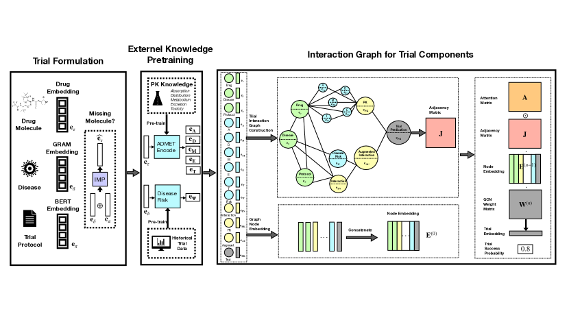
Figure 1: HINT extracts features from the following trial components: drug molecule embedding $\mathbf{e}_{\tau}$, disease embedding $\mathbf{e}_{\delta}$, and trial protocol embedding $\mathbf{e}_{\pi}$ (as described in section 3.1). Before constructing an interaction graph using these components, HINT pretrains certain embeddings (depicted as blue nodes) using external knowledge about medication characteristics and disease risks(Section 3.2). Subsequently, we create an interaction graph in Section 3.3 to depict the interactions among different trial components. Using this interaction graph, we obtain trial embeddings that represent the trial components and their interactions. Leveraging the learned embeddings and Dynamic Attentive Graph Neural Network (Eq. 15), we make predictions for trial outcomes.

3.1 Input Embedding Module

This module operates on a triad of data sources: (1) drug molecules, (2) disease information, and (3) trial protocols.

Drug molecules play a crucial role in forecasting the outcomes of clinical trials. These molecules are typically represented through SMILES strings or molecular graphs Zhang et al. (2021). Formally, treatment set $\mathcal{T}=\{\tau_{1},\cdots,\tau_{K_{\tau}}\}$ is represented as

$$\text{\text@underline{Drug Embedding}}\quad\mathbf{e}_{\tau}=\frac{1}{K_{\tau}}\sum_{i=1}^{K_{\tau}}g_{\tau}(\tau_{i})\in\mathbb{R}^{d},$$ (4)

where $g_{\tau}(\cdot)$ is designated as the molecule embedding function. By aggregating the molecular embeddings derived from a trial, we obtain drug embedding vector, which is conceptualized as the mean of all molecular embeddings Fu et al. (2022a). Our empirical investigations reveal that employing an averaging method as the aggregation mechanism for drug embeddings yields more effective results than utilizing a summative approach.

Disease information can significantly impact trial outcomes. For instance, oncology drugs exhibit lower approval rates compared to those for infectious diseases Hay et al. (2014); Gao et al. (2019); Fu et al. (2021). Disease information is primarily sourced from its descriptive texts and corresponding ontology, such as disease hierarchies like the International Classification of Diseases(ICD) Anker et al. (2016). Target Disease Set $\mathcal{D}=\{\delta_{1},\cdots,\delta_{K_{\delta}}\}$(Definition 2) in the trial can be represented as

$$\text{\text@underline{Disease Embedding}}\quad\ \mathbf{e}_{\delta}=\frac{1}{K_{\delta}}\sum_{j=1}^{K_{\delta}}G_{\delta}(\delta_{j})\in\mathbb{R}^{d},$$ (5)

where $G_{\delta}({\delta}_{j})$ represents an embedding of disease ${\delta}_{j}$ using GRAM (graph-based attention model) Choi and others (2017), which leverages the hierarchical information inherent to medical ontologies.

Trial protocol is a key document that outlines the conduct of a clinical trial and encompasses specific eligibility criteria essential for patient recruitment. These inclusion or exclusion criteria are systematically articulated in individual sentences. To effectively represent each sentence within these criteria, we utilize Clinical-BERT Alsentzer and others (2019). The derived sentence representations are then sequentially processed through 4 one-dimensional convolutional layers You et al. (2018), each layer employing varying kernel sizes to discern semantic nuances at four distinct levels of granularity. This is followed by a fully-connected layer that culminates in the formation of the protocol embedding. Concisely, the protocol embedding is characterized as

$$\text{\text@underline{Protocol Embedding}}\quad\ \mathbf{e}_{\pi}=g_{\pi}(\mathcal{P}),\ \ \ \ \mathbf{e}_{\pi}\in\mathbb{R}^{d}.$$ (6)

3.2 Pretraining Using External Knowledge

HINT integrates external knowledge sources to pretrain knowledge nodes and further refine and augment these input embeddings.

Pharmaco-kinetics Knowledge: We engage in the pretraining of embeddings by harnessing pharmaco-kinetic (PK) knowledge, which elucidates the body’s reaction to drug absorption. The efficacy of clinical trials is significantly influenced by factors such as the pharmacokinetic properties of a drug and the disease risk profile. In this process, we utilize a spectrum of publicly accessible PK experimental scores. Employing this data, our pretraining is directed toward predictive models for key ADMET (Absorption, Distribution, Metabolism, Excretion, Toxicity) properties. These properties are integral in drug discovery, offering vital insights into the comprehensive interaction of a drug with the human body Ghosh and others (2016); Gao et al. (2019):

(1) Absorption model quantifies the period of a drug’s absorption process within the human body.

(2) Distribution model evaluates how efficiently the drug molecules traverse the bloodstream and reach various bodily regions.

(3) Metabolism model assesses the active duration of the drug’s therapeutic effect.

(4) Excretion model gauges the effectiveness of the body in eliminating toxic elements of the drug.

(5) Toxicity model appraises the potential adverse effects a drug might have on the human body.

For each of these properties, we develop dedicated models to calculate their respective scores and latent embeddings. Our approach involves processing molecular inputs and generating binary outputs, which reflect the presence or absence of the desired ADMET property.

$$\text{\text@underline{ADMET}}\quad\begin{array}[]{l}\mathbf{e}_{*}=\Phi_{*}(\mathbf{e}_{\tau}),\ \ \hat{\omega}_{*}=\sigma(\mathrm{FCNN}(\mathbf{e}_{*}))\\ \min\ -{\omega}_{*}\log\hat{\omega}_{*}-(1-{\omega}_{*})\log(1-\hat{\omega}_{*})\\ \end{array}$$ (7)

where $\mathbf{e}_{\tau}\in\mathbb{R}^{d}$ is the input drug embedding defined in Eq. (4), ${\omega}_{*}\in\{0,1\}$ is the binary label, $*$ can be A, D, M, E, and T. $\mathrm{FCNN}$ is a one-layer fully connected neural network. $\sigma(\cdot)$ represents the Sigmoid function that maps the output of $\mathrm{FCNN}$ to the binary label ${\omega}_{*}$. $\Phi_{*}$ can be any neural network. Furthermore, we use highway neural network Srivastava et al. (2015), which is denoted as

$$\text{\text@underline{Highway Network}}\quad\mathbf{y}=\text{highway}(\mathbf{x}),\ \ \ \mathbf{y},\mathbf{x}\in\mathbb{R}^{d}.$$ (8)

This choice is motivated by the need to mitigate the vanishing gradient problem, a critical consideration in deep neural network training.

Disease risk embedding and trial risk prediction: Our model extends beyond drug properties, incorporating knowledge gleaned from historical data on trials related to the target diseases. We integrate information from various sources to assess disease risk: 1) Disease descriptions and their corresponding ontologies, and 2) Empirical data on historical trial success rates for each disease. We leverage detailed statistics on the success rates of diseases across different phases of clinical trials, as documented by Hay et al. (2014), which serve as a supervision signal for training our trial risk prediction model. More precisely, we utilize previous trial data, available at ClinicalTrials.gov, to predict the likelihood of success for upcoming trials based on the specific disorders involved. The predicted trial risk, denoted as $\hat{\omega}_{{\Psi}}$, and the embedding, $\mathbf{e}_{\Psi}\in\mathbb{R}^{d}$ are derived using a two-layer highway neural network (Eq. 8) ${\Psi}(\cdot)$:

$$\text{\text@underline{Disease Risk}}\begin{array}[]{l}\mathbf{e}_{\Psi}={\Psi}(\mathbf{e}_{\delta}),\ \ \hat{\omega}_{\Psi}={\sigma}(\mathrm{FCNN}(\mathbf{e}_{\Psi})),\\ \min-{\omega}_{\Psi}\log\hat{\omega}_{\Psi}-(1-{\omega}_{\Psi})\log(1-\hat{\omega}_{\Psi}),\\ \end{array}$$ (9)

where $\mathbf{e}_{\delta}\in\mathbb{R}^{d}$ is the input disease embedding in Eq. (5), $\hat{\omega}_{\Psi}\in[0,1]$ is the predicted trial risk between 0 and 1 (with 0 being the most likely to fail and 1 the most likely to succeed), and ${\omega}_{\Psi}\in\{0,1\}$ is the binary label indicating the success or failure of the trial as a function of disease only. $\mathrm{FCNN}$ is the one-layer fully connected layer. $\sigma(\cdot)$ represents the Sigmoid function that maps the output of $\mathrm{FCNN}$ to the binary label ${\omega}_{\Psi}$. Binary cross entropy loss between ${\omega}_{\Psi}$ and $\hat{\omega}_{\Psi}$ is used to guide the training.

3.3 Hierarchical Interaction Graph

(I). Trial Interaction Graph We have devised a hierarchical interaction graph, denoted as $\mathcal{H}$, which serves as the backbone for establishing connections among all input data sources and the crucial variables that exert influence over the outcomes of clinical trials. Below, we provide a comprehensive description of this interaction graph along with its initialization procedure. The interaction graph $\mathcal{H}$ is composed of four distinct tiers of nodes, each of which is intricately interconnected to reflect the intricate development process of real-world clinical trials. These tiers are as follows:

(1) Input nodes encompass drugs, target diseases, and trial protocols with node features of input embedding $\mathbf{e}_{\tau}$, $\mathbf{e}_{\delta},\mathbf{e}_{\pi}\in\mathbb{R}^{d}$, indicated in green in Figure 1 (Section 3.1).

(2) External knowledge nodes include ADMET embeddings $\mathbf{e}_{\text{A}},\mathbf{e}_{\text{D}},\mathbf{e}_{\text{M}},\mathbf{e}_{\text{E}},\mathbf{e}_{\text{T}}\in\mathbb{R}^{d}$, as well as disease risk embedding $\mathbf{e}_{\Psi}$. These representations are initialized with pretrained external knowledge and are indicated in blue in Figure 1 (Section 3.2).

(3) Aggregation nodes include (a) Interaction node $\mathbf{e}_{\text{IN}}$ connecting disease $\mathbf{e}_{\delta}$, drug molecules $\mathbf{e}_{\tau}$ and trial protocols $\mathbf{e}_{\pi}$; (b) Pharmaco-kinetics node $\mathbf{e}_{\text{PK}}$ connecting ADMET embeddings $\mathbf{e}_{\text{A}},\mathbf{e}_{\text{D}},\mathbf{e}_{\text{M}},\mathbf{e}_{\text{E}},\mathbf{e}_{\text{T}}$, $\mathbf{e}_{T}\in\mathbb{R}^{d}$ and (c) Augmented interaction node $\mathbf{e}_{\text{AU}}$ that augment the interaction node $\mathbf{e}_{\text{IN}}$ using disease risk node $\mathbf{e}_{\Psi}$. Aggregation nodes are indicated in yellow in Figure 1.

(4) Prediction node: $\mathbf{e}_{\text{PR}}$ node serves as the connection point between the Pharmaco-Kinetics node $\mathbf{e}_{\text{PK}}$ and the Augmented Interaction node $\mathbf{e}_{\text{AU}}$ for making predictions. It is represented in gray in Figure 1. The input nodes and external knowledge nodes have been previously detailed, and the resulting representations are utilized as node embeddings within the interaction graph. In the following sections, we elaborate on the aggregation nodes and the prediction nodes.

Aggregation nodes: The PK (Pharmaco-Kinetics) node aggregates information related to the five ADMET properties (Eq. 7). We obtain PK (Pharmaco-Kinetics) embedding as follows:

PK Embedding (10)

$$\mathbf{e}_{\text{PK}} =\mathcal{PK}(\mathbf{e}_{\text{A}},\mathbf{e}_{\text{D}},\mathbf{e}_{\text{M}},\mathbf{e}_{\text{E}},\mathbf{e}_{\text{T}}),$$

$$\mathbf{e}_{\text{PK}} \in\mathbb{R}^{d}.$$

Here, $\mathcal{PK}(\cdot)$ represents a one-layer fully-connected layer ( input dimension is $5*d$, output dimension is $d$ ) , whose input feature concatenating $\mathbf{e}_{\text{A}},\mathbf{e}_{\text{D}},\mathbf{e}_{\text{M}},\mathbf{e}_{\text{E}},\mathbf{e}_{\text{T}}$, followed by $d$-dimensional two-layer highway neural network (Eq. 8) Srivastava et al. (2015).

Next, we model the interaction among the input drug molecule, diseases, and protocols through an interaction node, and obtain its embedding as follows:

Interaction Embedding (11)

$$\mathbf{e}_{\text{IN}} =\mathcal{IN}(\mathbf{e}_{\tau},\mathbf{e}_{\delta},\mathbf{e}_{\pi}),$$

$$\mathbf{e}_{\text{IN}} \in\mathbb{R}^{d},$$

where $\mathbf{e}_{\tau},\mathbf{e}_{\delta},\mathbf{e}_{\pi}$ represent input embeddings defined in Eq. (4), Eq. (5) and Eq. (6), respectively. The neural architecture of $\mathcal{IN}(\cdot)$ consists of a one-layer fully-connected network (with input dimension is $3*d$ and output dimension is $d$) followed by a $d$-dimensional two-layer highway network (Eq. 8) Srivastava et al. (2015).

We also employ an augmented interaction model to combine (i) the trial risk associated with the target disease $\mathbf{e}_{\Psi}$ (Eq. 9) and (ii) the interaction among disease, molecule, and protocol represented by $\mathbf{e}_{\text{IN}}$ (Eq. 11).

$$\text{\text@underline{Augmented Interaction}}\ \ \ \ \mathbf{e}_{\text{AU}}=\mathcal{AU}({\mathbf{e}_{\Psi},\mathbf{e}_{\text{IN}}}),\ \mathbf{e}_{\text{AU}}\in\mathbb{R}^{d}.$$ (12)

Here $\mathcal{AU}(\cdot)$ is a one-layer fully connected network (with input dimension is $2*d$, output dimension is $d$) followed by a two-layer $d$-dimensional highway network (Eq. 8) Srivastava et al. (2015).

Prediction node synthesizes the Pharmaco-kinetics and the augmented interaction to derive the final prediction as follows:

$$\text{\text@underline{Trial Prediction}}\ \ \ \ \mathbf{e}_{\text{PR}}=\mathcal{PR}(\mathbf{e}_{\text{PK}},\mathbf{e}_{\text{AU}}),\ \mathbf{e}_{\text{PR}}\in\mathbb{R}^{d}.$$ (13)

Similar to $\mathcal{IN}()$ and $\mathcal{AU}()$, the architecture of $\mathcal{PR}$ consists of a one-layer fully connected network (with input dimension is $2*d$, output dimension is $d$) followed by a $d$-dimensional two-layer highway network (Eq. 8) Srivastava et al. (2015).

(II). Dynamic Attentive Graph Neural Network

Trial embeddings provide initial representations of different trial components and their interactions through a graph. To further enhance predictions, we design a dynamic attentive graph neural network that leverages this interaction graph to model influential trial components.

In mathematical terms, we consider the interaction graph $\mathcal{H}$ as the input graph, where nodes represent trial components, and edges denote relations among these components. We denote $\mathbf{J}\in\{0,1\}^{K\times K}$ as the adjacency matrix of $\mathcal{H}$. The node embeddings $\mathbf{E}^{(0)}$ are initialized by combining representations of all components as follows:

$$\mathbf{E}^{(0)}=[ \mathbf{e}_{\delta},\mathbf{e}_{\tau},\mathbf{e}_{\pi},\mathbf{e}_{\text{A}},\mathbf{e}_{\text{D}},\mathbf{e}_{\text{M}},\mathbf{e}_{\text{E}},\mathbf{e}_{\text{T}},\mathbf{e}_{\Psi},$$ (14)

$$\mathbf{e}_{{\text{PK}}},\mathbf{e}_{\text{IN}},\mathbf{e}_{\text{AU}},\mathbf{e}_{\text{PR}}]^{\top}\in\mathbb{R}^{K\times d},$$

$K=|\mathcal{H}|$ is the number of nodes in graph $\mathcal{H}$, and for this paper, $K=13$.

To enhance node embeddings, we utilize a graph convolutional network(GCN) Kipf and Welling (2017); Lu et al. (2019). The updating rule of GCN for the $n$-th layer is

$$\mathbf{E}^{(n)}=\text{RELU}\big{(}\mathbf{B}^{(n)}+(\mathbf{A}\odot\mathbf{J})(\mathbf{E}^{(n-1)}\mathbf{W}^{(n)})\big{)},$$ (15)

where $n=1,\cdots,N$, $N$ represents the depth of GCN. In the $n$-th layer, $\mathbf{E}^{(n)}\in\mathbb{R}^{K\times d}$ is node embedding, $\mathbf{B}^{(n)},\mathbf{W}^{(n)}\in\mathbb{R}^{K\times d}$ are the bias/weight parameter, $\odot$ denotes element-wise multiplication.

In contrast to the conventional GCN Kipf and Welling (2017), we introduce a learnable layer-independent attentive matrix $\mathbf{A}\in\mathbb{R}^{K\times K}_{+}$. $\mathbf{A}_{i,j}$, the ($i,j$)-th entry of $\mathbf{A}$, measures the importance of the edge connecting the $i$-th and $j$-th node in $\mathcal{H}$. We calculate $\mathbf{A}_{i,j}$ based on the embeddings of $i$-th and $j$-th nodes in $\mathbf{E}^{(0)}$, denoted as $\mathbf{e}^{i},\mathbf{e}^{j}\in\mathbb{R}^{d}$, ($\mathbf{e}^{i}\in\mathbb{R}^{d}$ is transpose of the $i$-th row of $\mathbf{E}^{(0)}\in\mathbb{R}^{K\times d}$ in Eq. 14).

$$\mathbf{A}_{i,j}=\mathcal{F}\big{(}[{\mathbf{e}^{i}}^{\top},{\mathbf{e}^{j}}^{\top}]^{\top}\big{)},\ \mathbf{A}_{i,j}>0$$ (16)

where $\mathcal{F}(\cdot)$ refers to a two-layer fully connected neural network with ReLU functions in the hidden layer and Sigmoid activation function in the output layer. Notably, the attentive matrix $\mathbf{A}$ is element-wise multiplied by the adjacency matrix $\mathbf{J}$ (as shown in Eq. 15) to ensure that edges with higher prediction scores are given more weight during message propagation.

Training After the message-passing phase in the GCN, we obtain updated representations for each trial component. These representations encode the essential information learned from the network. To predict trial success $\hat{\omega}$, we feed the final-layer ($N$-th layer) representation of the trial prediction node into a one-layer fully-connected network with a sigmoid activation function. We employ binary cross-entropy loss for training, which measures the dissimilarity between the predicted values and the true ground truth labels.

$$\hat{\omega}={\sigma}(\text{FCNN}(\mathbf{e}^{N}_{\text{PR}})).$$ (17)

$$\mathcal{L}_{\text{classify}}=-{\omega}\log\hat{\omega}-(1-{\omega})\log(1-\hat{\omega}).$$

In our case, ${\omega}\in\{0,1\}$ represents the ground truth, with ${\omega}=1$ indicating a successful trial and 0 indicating a failed one. HINT is trained in an end-to-end manner, optimizing its ability to predict trial outcomes based on the learned representations Fu and Sun (2022). $\sigma(\cdot)$ represents the Sigmoid function.

3.4 Missing Data Imputation

One significant challenge in handling trial data is the presence of missing molecular information $\mathcal{T}$, often due to proprietary reasons. In complete data scenario Wu et al. (2022), we have $(\mathcal{T},\mathcal{D},\mathcal{P},\omega)$, whereas with missing molecular data, we are left with only $(\mathcal{D},\mathcal{P},\omega)$. This becomes problematic as many node representations rely on molecular information. We’ve observed a strong correlation between drug molecules, diseases, and trial protocols. To address this issue, we design a missing data imputation module, denoted as $\text{IMP}(\cdot)$, which learns embeddings to capture inter-modal correlations and intra-modal distribution. In this study, the imputation module utilizes disease and protocol embeddings ($\mathbf{e}_{\delta},\mathbf{e}_{\pi}$) to recover the missing molecular embedding $\mathbf{e}_{\tau}$, as described in Eq. (18):

$$\widehat{\mathbf{e}_{\tau}}=\text{IMP}(\mathbf{e}_{\delta},\mathbf{e}_{\pi}).$$ (18)

To train this imputation module, we employ the Mean Square Error (MSE) loss Chen et al. (2021), aiming to minimize the difference between the predicted molecular embedding ($\widehat{\mathbf{e}_{\tau}}$) and the ground truth molecular embedding ($\mathbf{e}_{\tau}$):

$$\mathcal{L}_{\text{recovery}}=\|\widehat{\mathbf{e}_{\tau}}-{\mathbf{e}_{\tau}}\|_{2}^{2},$$ (19)

where $||\cdot||_{2}$ represents $l_{2}$-norm of a vector. During training, when dealing with complete data, we update $\text{IMP}(\cdot)$ via minimizing $\mathcal{L}_{\text{recovery}}$. In cases with missing data, we keep $\text{IMP}(\cdot)$ fixed and use $\widehat{\mathbf{e}_{\tau}}$ as a replacement for $\mathbf{e}_{\tau}$. We then proceed to update the remaining parts of the model.

4 Selective Classification to Quantify Uncertainty

Algorithm 1 HINT Framework with selective classification

1:  # 1. Pretrain

2:  Pretrain basic modules:   (i) ADMET models ($\mathcal{A},\mathcal{D},\mathcal{M},\mathcal{E},\mathcal{T}$);   (ii) disease risk (DR) model.

3:  Construct Interaction Graph $\mathcal{H}$.

4:  # 2. Train HINT on $\mathcal{X}_{train}$

5:  if complete data $(\mathcal{T},\mathcal{D},\mathcal{P},\omega)$ then

6:     Fix $\text{IMP}(\cdot)$ (Eq. 18), minimize $\mathcal{L}_{\text{classify}}$ (Eq. 17), update the remaining part of model.

7:     Minimize $\mathcal{L}_{\text{recover}}$ (Eq. 19), and only update $\text{IMP}(\cdot)$.

8:  else

9:     ### learn from missing data $(\mathcal{D},\mathcal{P},{\omega})$.

10:     Fix $\text{IMP}(\cdot)$, minimize $\mathcal{L}_{\text{classify}}$ (Eq. 17), update the remaining part of model.   

11:  end if

12:  # 3. Find threshold

13:  Specify $\alpha$, $\beta$, and the calibration set. Pick the threshold $\hat{\lambda}$ over the calibration set by the empirical selective accuracy (Eq. 21).

14:  # 4. Inference

15:  Given new data $(\mathcal{T},\mathcal{D},\mathcal{P})$, predict success probability $\hat{\omega}$.

16:  # 5. Classify selectively

17:  Output the prediction if $\max(\hat{\omega},1-\hat{\omega})$ exceeds $\hat{\lambda}$, otherwise abstains.

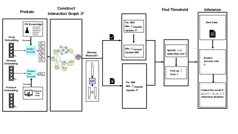
Figure 2: Selective Classification on HINT.

4.1 Problem Setting

We consider a binary classification problem, such as clinical trial outcome prediction, which HINT was designed to solve. Let $f:\mathcal{X}\rightarrow\mathcal{Y}$ be the model, with feature space $\mathcal{X}$ (e.g., trial embeddings) and label set $\mathcal{Y}=\{0,1\}$. Let $P(X,Y)$ be a joint distribution over $\mathcal{X}\times\mathcal{Y}$. The selective classifier $(f,g)$ is made up of the selective function $g:\mathcal{X}\rightarrow\{0,1\}$ and the classifier $f$, which produces a probability for each label provided in the input $x$.

$$\left.(f,g)(x)\triangleq\left\{\begin{array}[]{ll}f(x),&g(x)=1;\\ \text{abstain},&g(x)=0.\end{array}\right.\right.$$

Therefore, the prediction of input $x$ is abstained if $g(x)=0$. We measure the performance of a selective classifier using coverage and risk. Coverage is defined as the probability mass of the non-rejected region of $\mathcal{X}$, $\psi(f,g)=\mathbb{E}[g(X)]$. Given a loss function $\mathcal{L}$, the selective risk of (f, g) is defined as

$$\mathcal{R}(f,g)=\frac{\mathbb{E}[\mathcal{L}(f(x),y)g(x)]}{\psi(f,g)}.$$

4.2 Selective Classification (SC)

In many scenarios, it is preferable to display a model’s predictions only when it has high confidence. For instance, in medical diagnosis, we might only want the model to make predictions if it’s 90% certain, and if not, it should say, "I’m uncertain." The algorithm demonstrated below strategically abstains in order to achieve higher accuracy in clinical trial outcome prediction tasks.

More formally, given sample-label pairs $\{(X_{i},Y_{i})\}_{i=1}^{n}$ and a clinical trial outcome predictor $\hat{f}$ , we seek to ensure

$$\mathrm{P}(Y_{test}=\widehat{Y}(X_{test})\mid\widehat{P}(X_{test})\geq\hat{\lambda})\geq 1-\alpha,$$ (20)

where $\widehat{Y}(x)=\arg\max_{y}\hat{f}(x)_{y}$, $\widehat{P}(X_{test})=\max_{y}\hat{f}(x)_{y}$, and $\hat{\lambda}$ is a threshold chosen using the calibration data. This is called a selective accuracy guarantee because the accuracy is only computed over a subset of high-confidence predictions. We pick the threshold based on the empirical estimate of selective accuracy on the calibration set.

$$\begin{split}&\widehat{R}(\lambda)=\frac{1}{n(\lambda)}\sum_{i=1}^{n}{1}\left\{Y_{i}\neq\widehat{Y}(X_{i})\text{ and }\widehat{P}(X_{i})\geq\lambda\right\},\\ &\text{where }n(\lambda)=\sum_{i=1}^{n}{1}\left\{\widehat{P}(X_{i})\geq\lambda\right\}.\end{split}$$ (21)

where ${1}(\cdot)$ is an indicator function.

In particular, we will scan across values of $\lambda$, looking at a conservative upper bound for the true risk (i.e., the top end of a confidence interval for the selective misclassification rate). Realizing that $\widehat{R}(\lambda)$ is a Binomial random variable with $n(\lambda)$ trials, we upper-bound the misclassification error as

$$\widehat{R}^{+}(\lambda)=\sup\left\{r:\text{BinomCDF}(\widehat{R}(\lambda);n(\lambda),r)\geq\beta\right\}$$ (22)

for some user-specified failure rate $\beta\in[0,1]$. Then, scan the upper bound until the last time the bound exceeds $\alpha$,

$$\hat{\lambda}=\inf\left\{\lambda:\widehat{R}^{+}(\lambda^{\prime})\leq\alpha\text{ for all }\lambda^{\prime}\geq\lambda\right\}.$$ (23)

Using $\hat{\lambda}$ will satisfy Equation (20) with high probability.

5 Experiment

In our study, we utilized the TOP clinical trial outcome prediction benchmark, encompassing three phases.

5.1 Experiment Setting

Dataset. we employed the TOP clinical trial outcome prediction benchmark presented by Fu et al. (2022b, 2023). This dataset encompasses information on drugs, diseases, trial protocol, and trial outcomes for a total of 17,538 clinical experiments. These trials are categorized into three phases: Phase I with 1,787 trials, Phase II with 6,102 trials, and Phase III with 4,576 trials. Success rate differs across phases: 56.3% in Phase I, 49.8% in Phase II, and 67.8% in Phase III. A breakdown of the diseases targeted can be found in Table 1. Our research is executed distinctly in each phase of the trials.

Data Split. For data division, we followed Fu et al. (2022b, 2023) and split the dataset based on the registration date. The earlier trials are used for learning, while the later trials are used for inference. For instance, in Phase I, we trained the model on trials before Aug 13th, 2014, and tested on trials post this date, as shown in Table 1.

Table 1: Data statistics of clinical trial outcome prediction benchmark dataset presented by Fu et al. During training, we randomly select 15% training samples for model validation. The earlier trials are used for learning, while the later trials are used for inference. “Succ”, and “Fail” are abbreviations for success and failure, respectively.

Settings	Train		Test		Split Date
	Succ	Fail	Suss	Fail
Phase I	702	386	199	113	08/13/2014
Phase II	956	1655	302	487	03/20/2014
Phase III	1,820	2,493	457	684	04/07/2014

Evaluation Metrics: Our evaluation utilized various metrics such as PR-AUC, F1, ROC-AUC, and Accuracy. PR-AUC assesses the model’s ability to differentiate between positive and negative examples.

PR-AUC: (Area Under the Precision-Recall Curve). It quantifies the area under the precision-recall curve, representing how well the model separates positive and negative examples. PR-AUC focuses on the trade-off between precision (positive predictive value) and recall (true positive rate) across different probability thresholds.

Fl: The F1 score, represents the harmonic mean of precision and recall. The F1 score is a single metric combining precision and recall into a single value to assess a classification model’s performance. The F1 score adeptly balances the trade-off between precision (the accuracy of positive predictions) and recall (the ability to identify all positive instances), ensuring a more accurate evaluation of the model’s accuracy.

ROC-AUC: (Area Under the Receiver Operating Characteristic Curve) It focuses on the trade-off between true positive rate (TPR or recall) and false positive rate (FPR) across different probability thresholds. ROC-AUC quantifies the area under the ROC curve, which is a plot of TPR against FPR Lu et al. (2022). A higher ROC-AUC value indicates better model discrimination and the ability to distinguish between positive and negative examples.

Accuracy: The ratio of correct predictions to the total number of samples.

Furthermore, to promote transparency and facilitate reproducibility in the scientific community, we have made our code publicly available at the provided GitHub link .

5.2 Results

We conduct experiments to evaluate the effect of using selective classification (SC) on trial outcome prediction in the following aspects:

Table 2: Phase-Level Outcome Prediction

Phase I
	HINT	HINT with SC	Improvement
PR-AUC	0.5765±0.0119	0.7631±0.0119	32.37%
F1	0.6003±0.0091	0.7302±0.0091	21.64%
ROC-AUC	0.5723±0.0084	0.7164±0.0084	25.18%
Accuracy	0.5486±0.0046	0.6885±0.0083	25.50%
Retain rate	/	0.7874±0.0267	/

Phase II
	HINT	HINT with SC	Improvement
PR-AUC	0.6093±0.0131	0.7399±0.0055	21.43%
F1	0.6377±0.0110	0.7224±0.0036	13.28%
ROC-AUC	0.6191±0.0116	0.7299±0.0038	17.90%
Accuracy	0.5998±0.0052	0.7002±0.0031	16.74%
Retain rate	/	0.5414±0.0021	/

Phase III
	HINT	HINT with SC	Improvement
PR-AUC	0.7965±0.0092	0.9022±0.0031	13.27%
F1	0.8098±0.0093	0.8857±0.0048	9.37%
ROC-AUC	0.6843±0.0220	0.7735±0.0077	13.04%
Accuracy	0.7190±0.0063	0.8122±0.0059	18.69%
Retain rate	/	0.7117±0.0172	/

To discern the enhancement offered by selective classification over the conventional model, we conducted a phase-level outcome prediction. Each trial phase was modeled individually using pre-trained models from the HINT repository to ensure consistent and reproducible outcomes. We incorporated selective classification by setting a calibrated threshold $\lambda$ on the training set. This threshold acted as a decision boundary to either retain or abstain from predictions based on the model’s confidence, as indicated by the softmax output.

The detailed results and observations are presented in Table 2. The results reveal that: (1) We observed significant improvements across all phases, with Phase I showing the most notable improvements. This indicates a strong adaptability of our model to early-stage trials. (2) All key performance metrics demonstrated marked improvements. The most striking gains are observed in PR-AUC. Although the F1 score’s enhancements were comparatively modest, they are indicative of a meaningful improvement in the model’s ability to maintain a balance between precision and recall—a critical consideration in the realm of imbalanced clinical trial datasets.

The results indicate a tiered enhancement through the phases with selective classification (SC). Phase I trials show a remarkable 32.37% increase in PR-AUC, indicating a substantial boost in the model’s precision and recall trade-off. Phase II and III also show notable improvements, albeit less pronounced than Phase I. This could be due to the higher initial success rates in later phases, which leave less room for improvement. The data suggests that SC has the most significant impact where the uncertainty in predictions is greatest, thereby emphasizing the utility of SC in early-stage trials where risk assessment is critical.

6 Conclusion

In conclusion, our study utilizing the Hierarchical Interaction Network (HINT) has presented a transformative approach in the domain of clinical trial outcome prediction. By integrating the selective classification methodology, we have addressed and quantified the inherent model uncertainty, which has illustrated marked enhancements in performance.

The empirical results are compelling, demonstrating that selective classification confers a significant advantage, particularly evidenced by the pronounced improvements in PR-AUC across all phases of clinical trials. This is indicative of a more discerning model, capable of delivering higher precision in its predictions, especially in the critical early phases of clinical development.

The selective classification’s impact is most striking in Phase I trials, where the model’s adaptability is crucial due to the higher uncertainty and variability. Despite the smaller gains in the F1 score, the consistent uplift across all metrics, including ROC AUC and accuracy, underscores the overall increase in the model’s predictive reliability.

This work paves the way for future explorations into more nuanced models that can handle the complexities of clinical trial data, offering a beacon for forthcoming research in the field. Our findings advocate for the continued development and refinement of models like HINT, emphasizing the need for precision and care in predictive analytics within clinical research. The potential for these advancements can significantly impact patient outcomes and improve the efficiency of trial design.

References

- Alsentzer and others [2019] Emily Alsentzer et al. Publicly available clinical BERT embeddings. arXiv:1904.03323, 2019.
- Anker et al. [2016] Stefan D Anker, John E Morley, and Stephan von Haehling. Welcome to ICD-10 code for sarcopenia. Journal of cachexia, sarcopenia and muscle, 2016.
- Bartlett and Wegkamp [2008] Peter L Bartlett and Marten H Wegkamp. Classification with a reject option using a hinge loss. Journal of Machine Learning Research, 9(8), 2008.
- Chen et al. [2021] Lulu Chen, Yingzhou Lu, Chiung-Ting Wu, Robert Clarke, Guoqiang Yu, Jennifer E Van Eyk, David M Herrington, and Yue Wang. Data-driven detection of subtype-specific differentially expressed genes. Scientific reports, 11(1):332, 2021.
- Choi and others [2017] Edward Choi et al. GRAM: graph-based attention model for healthcare representation learning. In KDD, 2017.
- Chow [1957] Chi-Keung Chow. An optimum character recognition system using decision functions. IRE Transactions on Electronic Computers, (4):247–254, 1957.
- Chow [1970] C Chow. On optimum recognition error and reject tradeoff. IEEE Transactions on information theory, 16(1):41–46, 1970.
- De et al. [2020] Abir De, Paramita Koley, Niloy Ganguly, and Manuel Gomez-Rodriguez. Regression under human assistance. In Proceedings of the AAAI Conference on Artificial Intelligence, volume 34, pages 2611–2620, 2020.
- El-Yaniv and others [2010] Ran El-Yaniv et al. On the foundations of noise-free selective classification. Journal of Machine Learning Research, 11(5), 2010.
- Feng et al. [2019] Jean Feng, Arjun Sondhi, Jessica Perry, and Noah Simon. Selective prediction-set models with coverage guarantees. arXiv preprint arXiv:1906.05473, 2019.
- Friedman et al. [2015] Lawrence M Friedman, Curt D Furberg, David L DeMets, David M Reboussin, and Christopher B Granger. Fundamentals of clinical trials. Springer, 2015.
- Fu and Sun [2022] Tianfan Fu and Jimeng Sun. Antibody complementarity determining regions (cdrs) design using constrained energy model. In Proceedings of the 28th ACM SIGKDD Conference on Knowledge Discovery and Data Mining, pages 389–399, 2022.
- Fu et al. [2021] Tianfan Fu, Wenhao Gao, Cao Xiao, Jacob Yasonik, Connor W Coley, and Jimeng Sun. Differentiable scaffolding tree for molecular optimization. arXiv preprint arXiv:2109.10469, 2021.
- Fu et al. [2022a] Tianfan Fu, Wenhao Gao, Connor Coley, and Jimeng Sun. Reinforced genetic algorithm for structure-based drug design. Advances in Neural Information Processing Systems, 35:12325–12338, 2022.
- Fu et al. [2022b] Tianfan Fu, Kexin Huang, Cao Xiao, Lucas M Glass, and Jimeng Sun. Hint: Hierarchical interaction network for clinical-trial-outcome predictions. Patterns, 3(4), 2022.
- Fu et al. [2023] Tianfan Fu, Kexin Huang, and Jimeng Sun. Automated prediction of clinical trial outcome, February 2 2023. US Patent App. 17/749,065.
- Gal and Ghahramani [2016] Yarin Gal and Zoubin Ghahramani. Dropout as a bayesian approximation: Representing model uncertainty in deep learning. In international conference on machine learning, pages 1050–1059. PMLR, 2016.
- Gao et al. [2019] Tian Gao, Cao Xiao, Tengfei Ma, and Jimeng Sun. Pearl: Prototype learning via rule learning. In Proceedings of the 10th ACM International Conference on Bioinformatics, Computational Biology and Health Informatics, pages 223–232, 2019.
- Geifman and El-Yaniv [2017] Yonatan Geifman and Ran El-Yaniv. Selective classification for deep neural networks. Advances in neural information processing systems, 30, 2017.
- Geifman and El-Yaniv [2019] Yonatan Geifman and Ran El-Yaniv. Selectivenet: A deep neural network with an integrated reject option. In International conference on machine learning, pages 2151–2159. PMLR, 2019.
- Ghosh and others [2016] Jayeeta Ghosh et al. Modeling admet. In Silico Methods for Predicting Drug Toxicity. 2016.
- Hay et al. [2014] Michael Hay, David W Thomas, John L Craighead, Celia Economides, and Jesse Rosenthal. Clinical development success rates for investigational drugs. Nat. Biotechnol., 2014.
- Hellman and Raviv [1970] Martin Hellman and Josef Raviv. Probability of error, equivocation, and the chernoff bound. IEEE Transactions on Information Theory, 16(4):368–372, 1970.
- Hellman [1970] Martin E Hellman. The nearest neighbor classification rule with a reject option. IEEE Transactions on Systems Science and Cybernetics, 6(3):179–185, 1970.
- Hong et al. [2020] Zhen Yu Hong, Jooyong Shim, Woo Chan Son, and Changha Hwang. Predicting successes and failures of clinical trials with an ensemble ls-svr. medRxiv, 2020.
- Khani et al. [2016] Fereshte Khani, Martin Rinard, and Percy Liang. Unanimous prediction for 100% precision with application to learning semantic mappings. arXiv preprint arXiv:1606.06368, 2016.
- Kipf and Welling [2017] Thomas N Kipf and Max Welling. Semi-supervised classification with graph convolutional networks. ICLR, 2017.
- Lakshminarayanan et al. [2017] Balaji Lakshminarayanan, Alexander Pritzel, and Charles Blundell. Simple and scalable predictive uncertainty estimation using deep ensembles. Advances in neural information processing systems, 30, 2017.
- Ledford [2011] Heidi Ledford. 4 ways to fix the clinical trial: clinical trials are crumbling under modern economic and scientific pressures. nature looks at ways they might be saved. Nature, 2011.
- Lo et al. [2019] Andrew W Lo, Kien Wei Siah, and Chi Heem Wong. Machine learning with statistical imputation for predicting drug approvals, volume 60. SSRN, 2019.
- Lu et al. [2019] Yingzhou Lu, Yi-Tan Chang, Eric P Hoffman, Guoqiang Yu, David M Herrington, Robert Clarke, Chiung-Ting Wu, Lulu Chen, and Yue Wang. Integrated identification of disease specific pathways using multi-omics data. bioRxiv, page 666065, 2019.
- Lu et al. [2022] Yingzhou Lu, Chiung-Ting Wu, Sarah J Parker, Zuolin Cheng, Georgia Saylor, Jennifer E Van Eyk, Guoqiang Yu, Robert Clarke, David M Herrington, and Yue Wang. Cot: an efficient and accurate method for detecting marker genes among many subtypes. Bioinformatics Advances, 2(1):vbac037, 2022.
- Lu et al. [2023] Yingzhou Lu, Huazheng Wang, and Wenqi Wei. Machine learning for synthetic data generation: a review. arXiv preprint arXiv:2302.04062, 2023.
- Martin et al. [2017] Linda Martin, Melissa Hutchens, Conrad Hawkins, and Alaina Radnov. How much do clinical trials cost? Nat. Rev. Drug Discov., 2017.
- Mozannar and Sontag [2020] Hussein Mozannar and David Sontag. Consistent estimators for learning to defer to an expert. In International Conference on Machine Learning, pages 7076–7087. PMLR, 2020.
- Papadopoulos et al. [2002] Harris Papadopoulos, Kostas Proedrou, Volodya Vovk, and Alex Gammerman. Inductive confidence machines for regression. In Machine Learning: ECML 2002: 13th European Conference on Machine Learning Helsinki, Finland, August 19–23, 2002 Proceedings 13, pages 345–356. Springer, 2002.
- Peto [1978] Richard Peto. Clinical trial methodology. Nature, 1978.
- Qi and Tang [2019] Youran Qi and Qi Tang. Predicting phase 3 clinical trial results by modeling phase 2 clinical trial subject level data using deep learning. Proceedings of Machine Learning Research, 2019.
- Raghu et al. [2019] Maithra Raghu, Katy Blumer, Rory Sayres, Ziad Obermeyer, Bobby Kleinberg, Sendhil Mullainathan, and Jon Kleinberg. Direct uncertainty prediction for medical second opinions. In International Conference on Machine Learning, pages 5281–5290. PMLR, 2019.
- Rajpurkar and others [2020] Pranav Rajpurkar et al. Evaluation of a Machine Learning Model Based on Pretreatment Symptoms and Electroencephalographic Features to Predict Outcomes of Antidepressant Treatment in Adults With Depression: A Prespecified Secondary Analysis of a Randomized Clinical Trial. JAMA Network Open, 2020.
- Research [2021] Grand View Research. Clinical trials market size, share & trends analysis report by phase (phase i, phase ii, phase iii, phase iv), by study design (interventional, observational, expanded access), by indication, by region, and segment forecasts 2021–2028, 2021.
- Srivastava et al. [2015] Rupesh Kumar Srivastava, Klaus Greff, and Jürgen Schmidhuber. Training very deep networks. In NIPS, 2015.
- Vijayananthan and Nawawi [2008] Anushya Vijayananthan and Ouzreiah Nawawi. The importance of good clinical practice guidelines and its role in clinical trials. Biomedical imaging and intervention journal, 4(1), 2008.
- Vovk et al. [2005] Vladimir Vovk, Alexander Gammerman, and Glenn Shafer. On-line compression modeling i: conformal prediction. Algorithmic learning in a random world, pages 189–221, 2005.
- Wang et al. [2022] Zifeng Wang, Chufan Gao, Lucas M Glass, and Jimeng Sun. Artificial intelligence for in silico clinical trials: A review. arXiv preprint arXiv:2209.09023, 2022.
- Wu et al. [2022] Chiung-Ting Wu, Minjie Shen, Dongping Du, Zuolin Cheng, Sarah J Parker, Yingzhou Lu, Jennifer E Van Eyk, Guoqiang Yu, Robert Clarke, David M Herrington, et al. Cosbin: cosine score-based iterative normalization of biologically diverse samples. Bioinformatics Advances, 2(1):vbac076, 2022.
- Yi et al. [2018] Steven Yi, Minta Lu, Adam Yee, John Harmon, Frank Meng, and Saurabh Hinduja. Enhance wound healing monitoring through a thermal imaging based smartphone app. In Medical Imaging 2018: Imaging Informatics for Healthcare, Research, and Applications, volume 10579, pages 438–441. SPIE, 2018.
- You et al. [2018] Quanzeng You, Zhengyou Zhang, and Jiebo Luo. End-to-end convolutional semantic embeddings. In CVPR, 2018.
- Zhang et al. [2021] Bai Zhang, Yi Fu, Yingzhou Lu, Zhen Zhang, Robert Clarke, Jennifer E Van Eyk, David M Herrington, and Yue Wang. Ddn2. 0: R and python packages for differential dependency network analysis of biological systems. bioRxiv, pages 2021–04, 2021.