11institutetext: Vivekanand Dabade 22institutetext: Department of Aerospace Engineering
Indian Institute of Science
Bengaluru, India
22email: dabade@iisc.ac.in

Deformation of a planar ferromagnetic elastic ribbon

G. R. Krishna Chand Avatar    Vivekanand Dabade
(Received: date / Accepted: date)
Abstract

While extensive studies have been conducted on purely elastic ribbons, in this paper we explore the influence of magnetisation on the deformation of planar ferromagnetic elastic ribbons. We begin the investigation by deriving the leading-order magnetic energy associated with a curved planar ferromagnetic elastic ribbon. The sum of the magnetic and the elastic energy is the total energy of the ribbon. We derive the equilibrium equations by taking the first variation of the total energy. We then systematically determine and analyse solutions to these equilibrium equations under various canonical boundary conditions. We also analyse the stability of the equilibrium solutions. Comparing our findings with the well-studied Euler’s Elastica provides insights into the magnetic effects on the deformation behaviour of elastic ribbons. Our analysis contributes to a deeper understanding of the interplay between magnetisation and the mechanical response of planar ferromagnetic structures, and offers valuable insights for both theoretical and practical applications.

Keywords:
Magnetoelastic slender structures Soft ferromagnets Hard ferromagnets Ribbons Elastica
MSC:
MSC code1 MSC code2 more
journal: Journal of Elasticity

1 Introduction

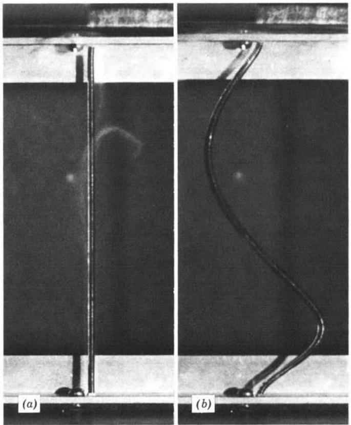
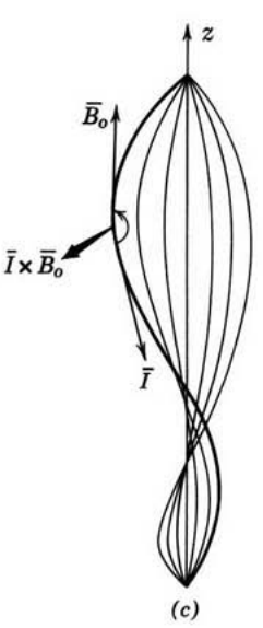
Magneto-elastic slender structures exhibit complex coupling between magnetism and deformation or elasticity. A fascinating experiment conducted in the late 1960s demonstrated the intriguing connection between deformation and magnetism in a mechanical spring that carries an electric current and is placed in an external magnetic field, see Fig. 1. Under the influence of a tensile load, the spring undergoes buckling, underscoring the complexity of this coupling phenomenon. Slender ferromagnetic structures offer the potential to achieve substantial deformations using remote external magnetic fields. This complex coupling is being applied in ferromagnetic continuum robots, innovative actuators, and remotely controlled minimally invasive surgeries, kim2019ferromagnetic ; Ramachandran2016 .
Refer to caption
Refer to caption
Figure 1: (a) A conducting spring, elongated between the poles of a electromagnet, serves as the experimental configuration. (b) The onset of instability occurs after the electromagnet is turned on. (c) Schematic of the first mode of instability. Here, I𝐼I is the current flowing through the spring and 𝑩osubscript𝑩𝑜{\bf\it B}_{o} is the magnetic flux density due to the electromagnet. Note that the spring buckles under tensile force. Source: Woodson_Melcher_1985 .

Purely magnetic slender structures desimone2002reduced and purely elastic slender structures Audoly2010elasticity have each been studied separately in great detail. The study of elastic slender structures dates back to Euler, who obtained the deformation of an elastic planar rod. These deformations are represented by a family of planar curves using elliptic functions and is known as Euler’s Elastica. Elastica finds applications ranging from the modelling of DNA loops to laying of ocean cables and design of elastic robots, see balaeff2006modeling ; coyne1990analysis ; handral2020elastica ; armanini2017elastica . There have also been fairly recent studies concerning the stability of the solutions to the Elastica, see maddocks1984stability and kuznetsov2002complete .

Similarly, there have been extensive studies on ferromagnetic thin films and straight rods in the field of micromagnetics, desimone2002reduced ; Slastikov2011 . Micromagnetics is a continuum theory for magnetism that has proven to be a robust model capable of explaining and predicting the diverse array of domain structures observed in ferromagnetic materials. These studies consider the ferromagnetic slender structure without deformation and delineate the role of aspect ratio on the formation of the observed magnetic domain structures. The magnetisation vector 𝒎(𝒙)𝒎𝒙{\bf\it m}({\bf\it x}) is the primary variable in the micromagnetics functional. 𝒎(𝒙)𝒎𝒙{\bf\it m}({\bf\it x}) is a unit-normed vector supported on a ferromagnetic body. The micromagnetic functional is expressed as the sum of exchange, magnetocrystalline anisotropy, magnetostatic (abbreviated as demag.), and Zeeman energy, dabade2019micromagnetics . In particular, the demag. energy, strongly depends on the shape of the body and is computed by solving Maxwell’s equations of magnetostatics. The demag. energy is computationally expensive and is difficult to calculate for general 3D bodies but takes simpler forms for slender structures. This gives us an opportunity to explore these problems (semi-) analytically and hence, the demag. energy will play a crucial role in our analysis.

There has been limited research dedicated to understand the coupling between magnetisation and deformation in thin ferromagnetic structures. Bulk ferromagnetic solids (Iron, Nickel, Galfenol etc.) are known to deform when magnetised. This phenomenon is known as Joule magnetostriction. However, even under strong external magnetic fields, magnetostriction strains are small, typically in the order of 105superscript10510^{-5}. Our work does not consider Joule magnetostriction, we are primarily interested in understanding the deformation in slender ferromagnetic structures due to the effects of demag. energy and Zeeman energy. The elastic energy and magnetic energy are comparable in slender ferromagnetic structures, even though the elastic energy density is typically much greater than the magnetic energy density in bulk ferromagnetic materials. Hence, we can obtain large displacements in ferromagnetic slender structures while the strains in bulk ferromagnetic solids due to Joule magnetostriction are very small.

In bulk ferromagnetic materials, the elastic energy density scales as E(1011J/m3)annotated𝐸similar-toabsentsuperscript1011𝐽superscript𝑚3E\leavevmode\nobreak\ (\sim 10^{11}J/m^{3}), whereas the demag. energy scales as Kd(105J/m3)annotatedsubscript𝐾𝑑similar-toabsentsuperscript105𝐽superscript𝑚3K_{d}\leavevmode\nobreak\ (\sim 10^{5}J/m^{3}). Here, Kdsubscript𝐾𝑑K_{d} and E𝐸E represent the magnetostatic energy constant and Young’s modulus of the material, respectively, with both being material parameters. However, in slender structures the elastic energy and the demag. energy density scale very differently with respect to the aspect ratio. The leading-order demag. energy of a slender ferromagnetic ribbon scales as 𝒪(Kdatl)𝒪subscript𝐾𝑑𝑎𝑡𝑙\mathcal{O}(K_{d}atl), and the elastic energy scales as 𝒪(EI2l)𝒪𝐸𝐼2𝑙\mathcal{O}\left(\frac{EI}{2l}\right). Here, thickness, width, and length of the ferromagnetic ribbon are denoted as t𝑡t, a𝑎a, and l𝑙l, respectively, and I=bt312𝐼𝑏superscript𝑡312I=\frac{bt^{3}}{12}, is the area moment of inertia, see Fig 2. Hence, ferromagnetic slender structures offer an opportunity to tune the aspect ratio, allowing the interaction between demag. energy and elastic energy. A balance of these energies implies that our analysis is valid for ribbons with an aspect ratio of 𝒪(E24Kd)𝒪𝐸24subscript𝐾𝑑\mathcal{O}\left(\sqrt{\frac{E}{24K_{d}}}\right).

In our article, we explore the interaction between elasticity and magnetism in the simplest setting. Our analysis focuses on the deformation of a slender body resulting from the interplay of demag. energy and Zeeman energy, collectively referred to as magnetic energy, along with elastic energy. We consider a ferromagnetic ribbon, that is, a planar ribbon or rod composed of a ferromagnetic material such as Iron or Nickel. In particular, we shall study the two following cases:

  • Case 1. (Soft ferromagnet) : Magnetisation vector 𝒎(𝒙)𝒎(𝒙){\bf\it m(x)} is spatially constant and does not change with deformation. This case characterises soft ferromagnetic materials such as Permalloy, with an external magnetic field large enough to saturate the magnetisation uniformly throughout the deformed planar ribbon.

  • Case 2. (Hard ferromagnet) : Magnetisation vector 𝒎(𝒙)𝒎(𝒙){\bf\it m(x)} makes a constant angle with respect to the tangent of the deformed planar curve. Here, the tangent vector, and hence the magnetisation vector vary spatially as the slender body undergoes deformation. This case characterises hard ferromagnetic materials such as Neodymium or Samarium-Cobalt.

The total energy of a ferromagnetic slender ribbon is given by the sum of the elastic energy, magnetic energy of the ribbon and energy due to mechanical loading device. We shall consider the ribbon to be inextensible and hence the elastic energy is given by its bending energy. The magnetic energy is formulated based on the principles of micromagnetics. The magnetic energy is equal to the sum of the demag. energy and the Zeeman energy. We obtain the demag. energy for a curved ferromagnetic ribbon by employing a local material frame aligned with the tangent line of the deformed curve. Working in the deformed configuration alleviates the need to define a pull-back for the magnetisation vector 𝒎(𝒙)𝒎(𝒙){\bf\it m(x)} and solving the Maxwell’s equations of magnetostatics in the reference configuration. Various pullbacks for magnetisation are defined in the literature, posing challenges in the rational selection of the appropriate one, James2002 ; Keip2019 . The leading order demag. energy is local in nature and hence amenable for analysis. Calculating the remaining component of the magnetic energy, namely the Zeeman energy of the ribbon, is straightforward.

We determine the deformed configuration by solving the equilibrium equations obtained by taking the first variation of the total energy. The equilibrium equations show that the magnetisation produces a body couple along the length of the curve that is dependent on the local orientation of the curve, in addition to the conventional terms originating from elastic energy, see Eqn. 25. The equilibrium equations are solved numerically for various canonical boundary conditions, using Auto-07p, a standard software used in continuation and bifurcation problems Doedel1991a ; Doedel1991b . Further, we also perform a stability analysis of our computed solutions. The stability analysis involves casting the second variation of the total energy as a Sturm-Liouville boundary value problem. The eigenvalues of this boundary value problem, as the load is varied continuously, are used to determine the stability of the deformed configurations.

We obtain the equilibrium path and the stability of the first few relevant modes, under quasi-static load control simulation. Our results provide us with a stable deformed state of the ferromagnetic ribbon, beginning from zero load and, in certain instances, a moderate tensile load, and extending to an arbitrarily large compressive load. The main findings from our analysis are as follows:

Case 1: Soft ferromagnetic ribbon:

\bullet 

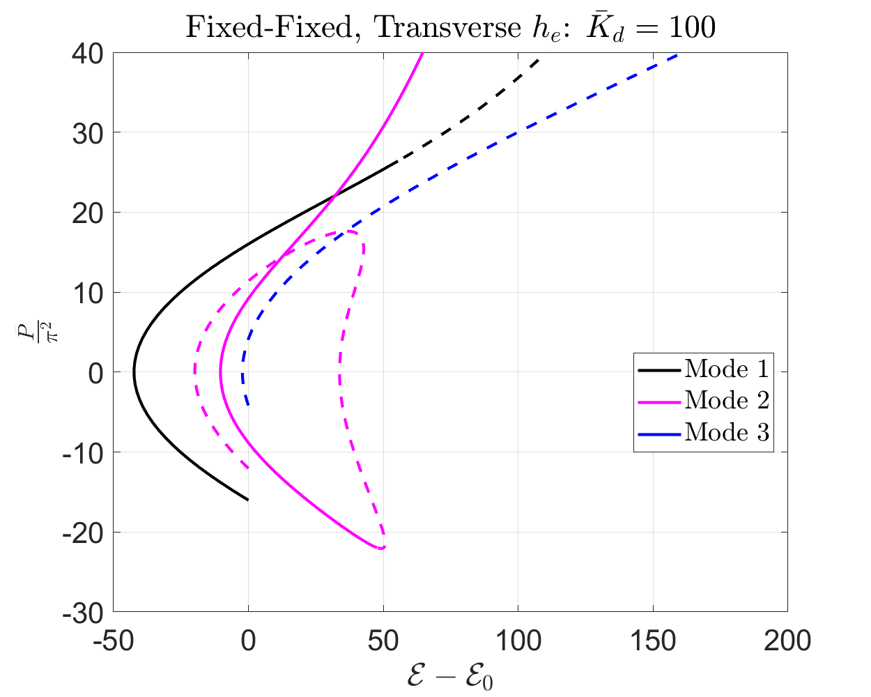
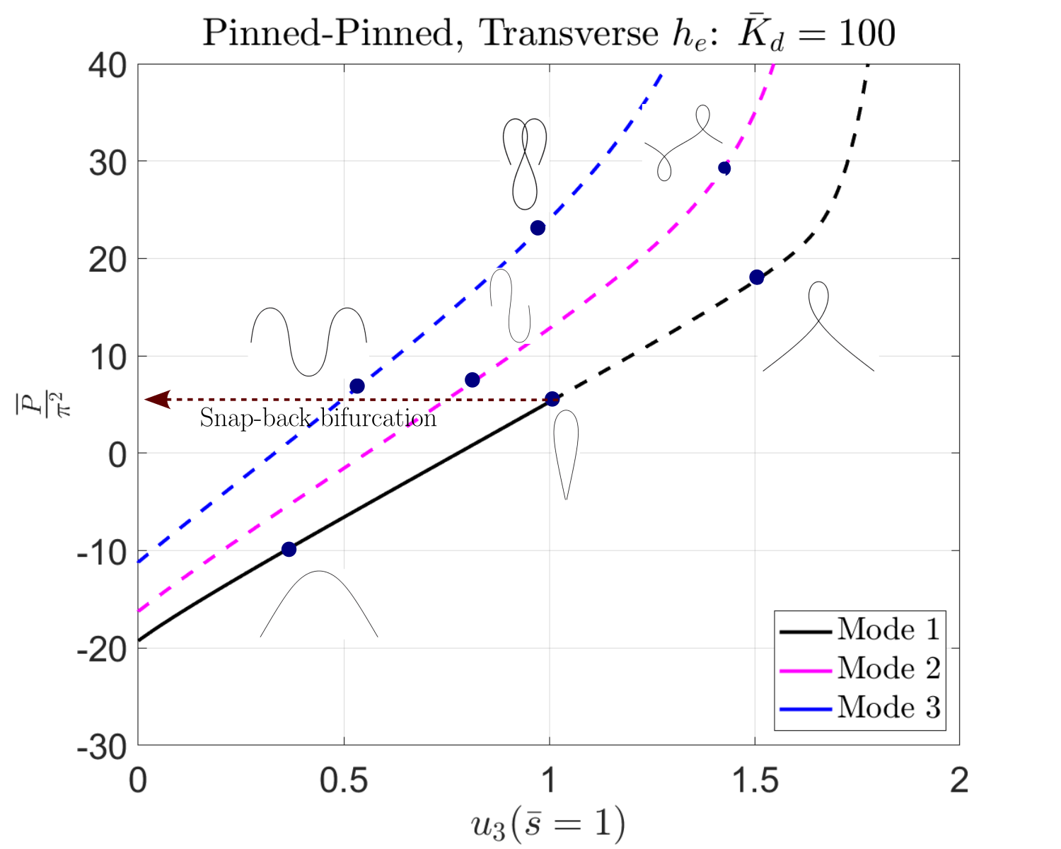
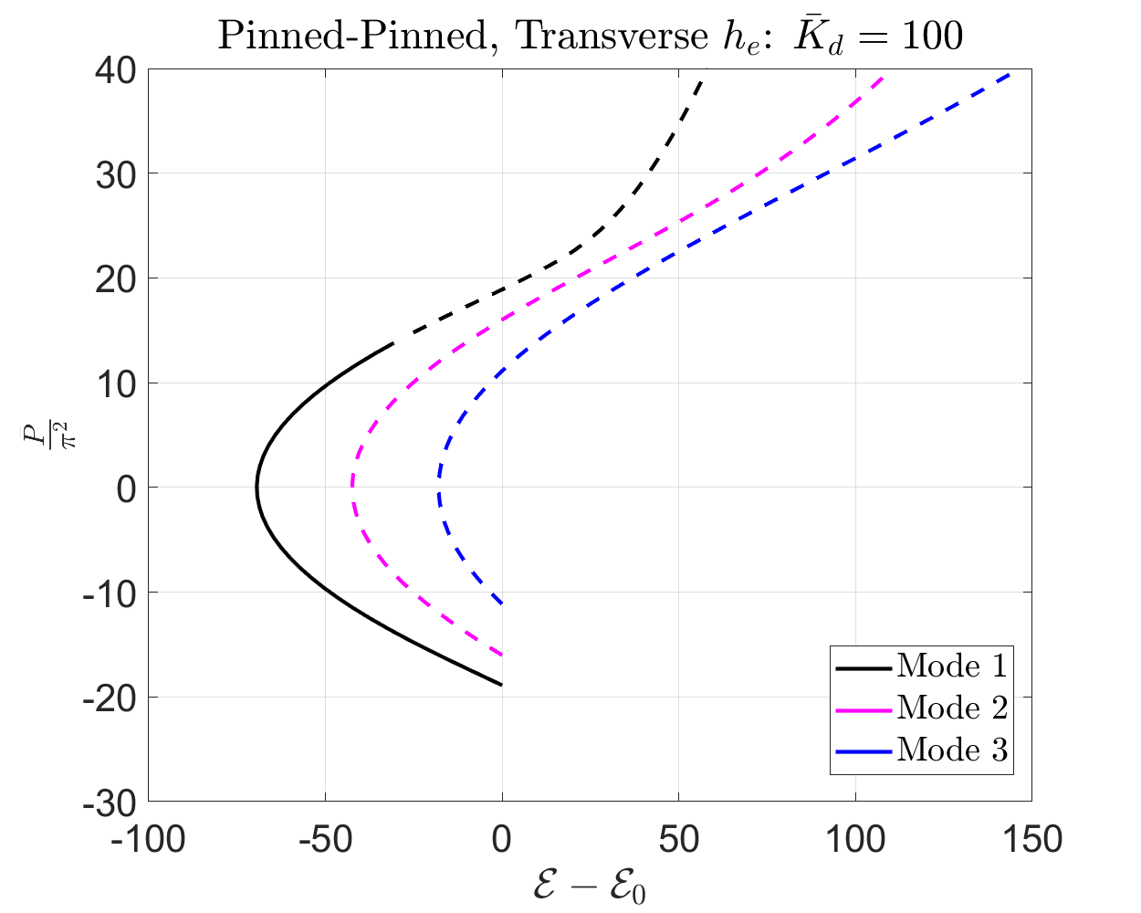
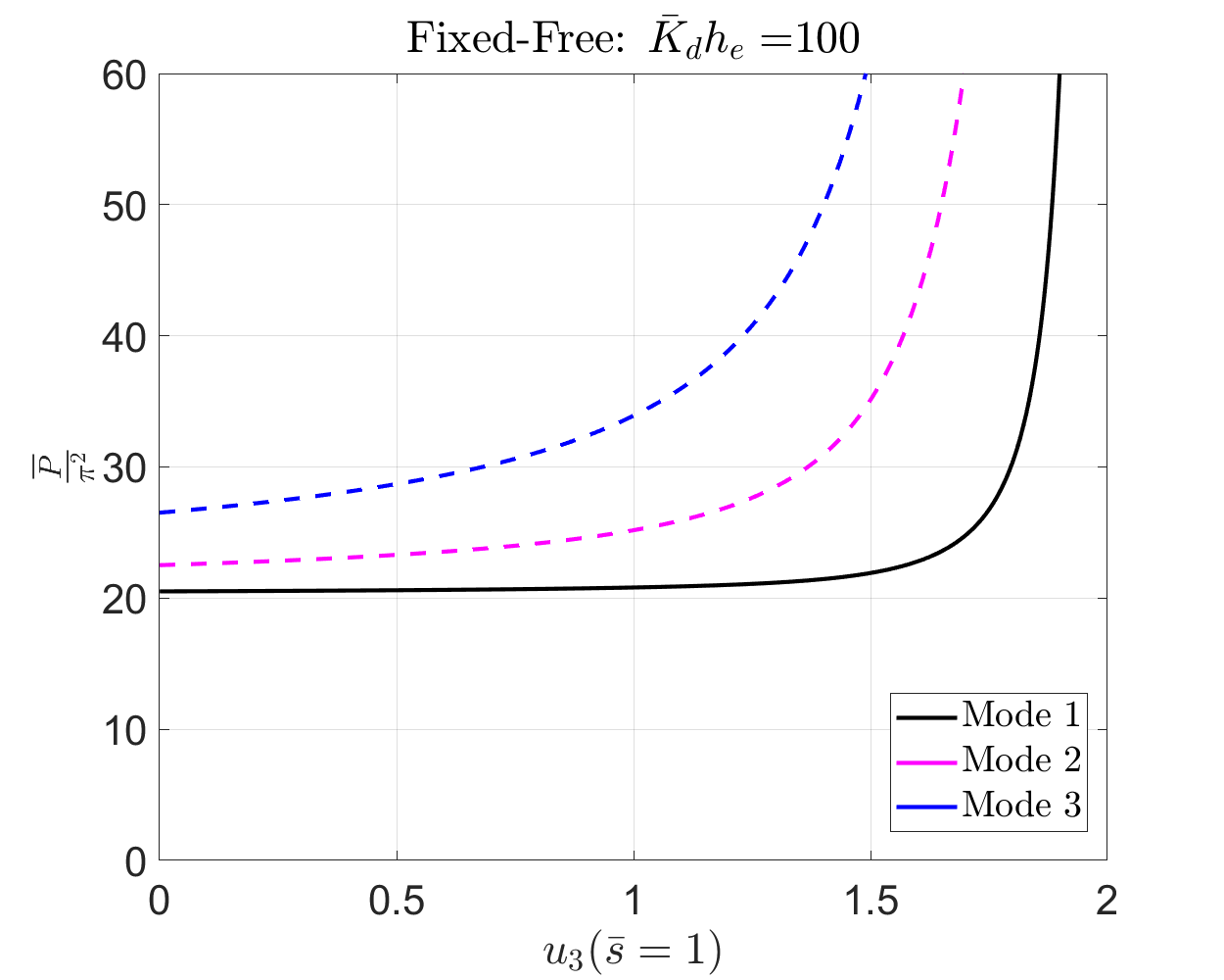
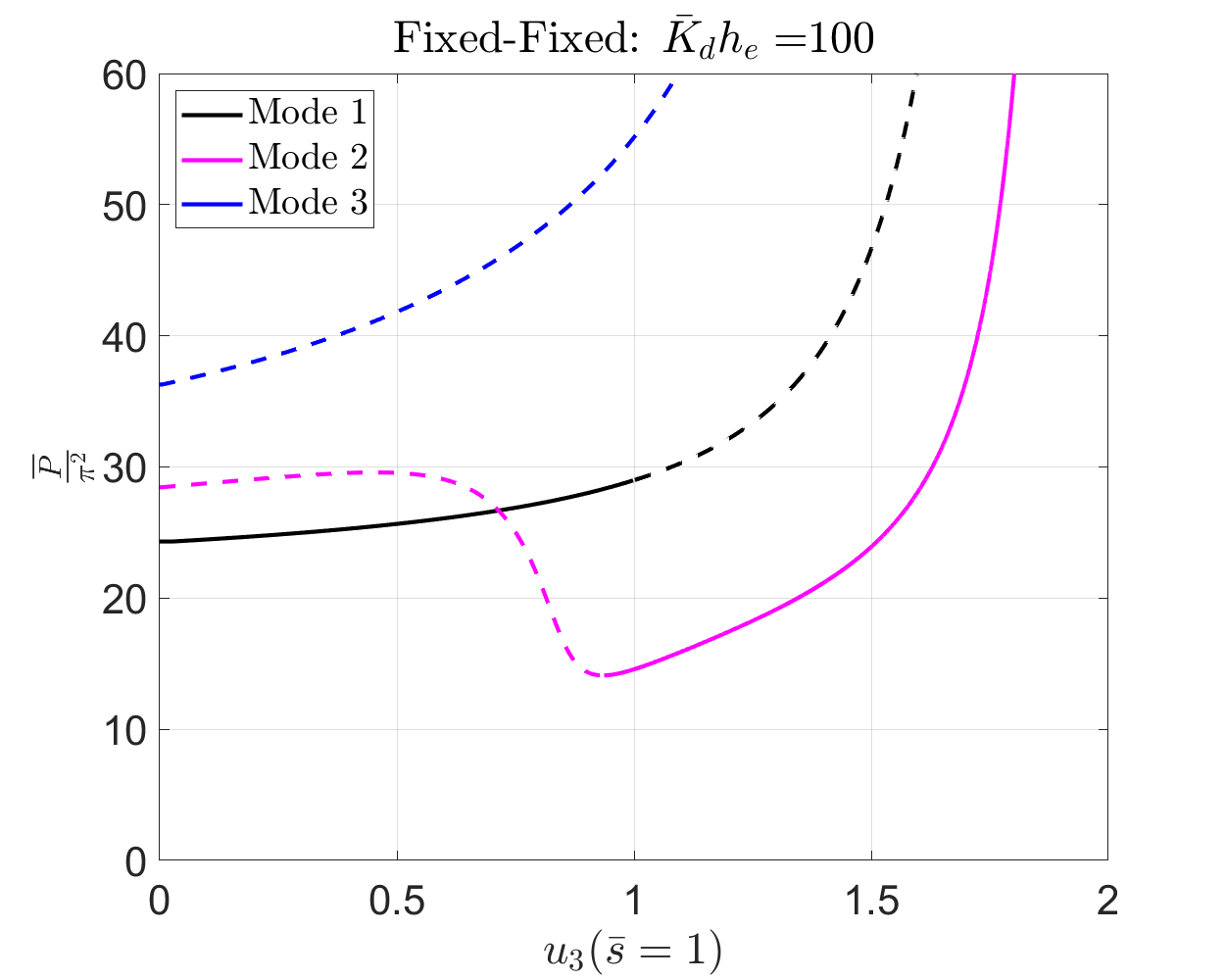
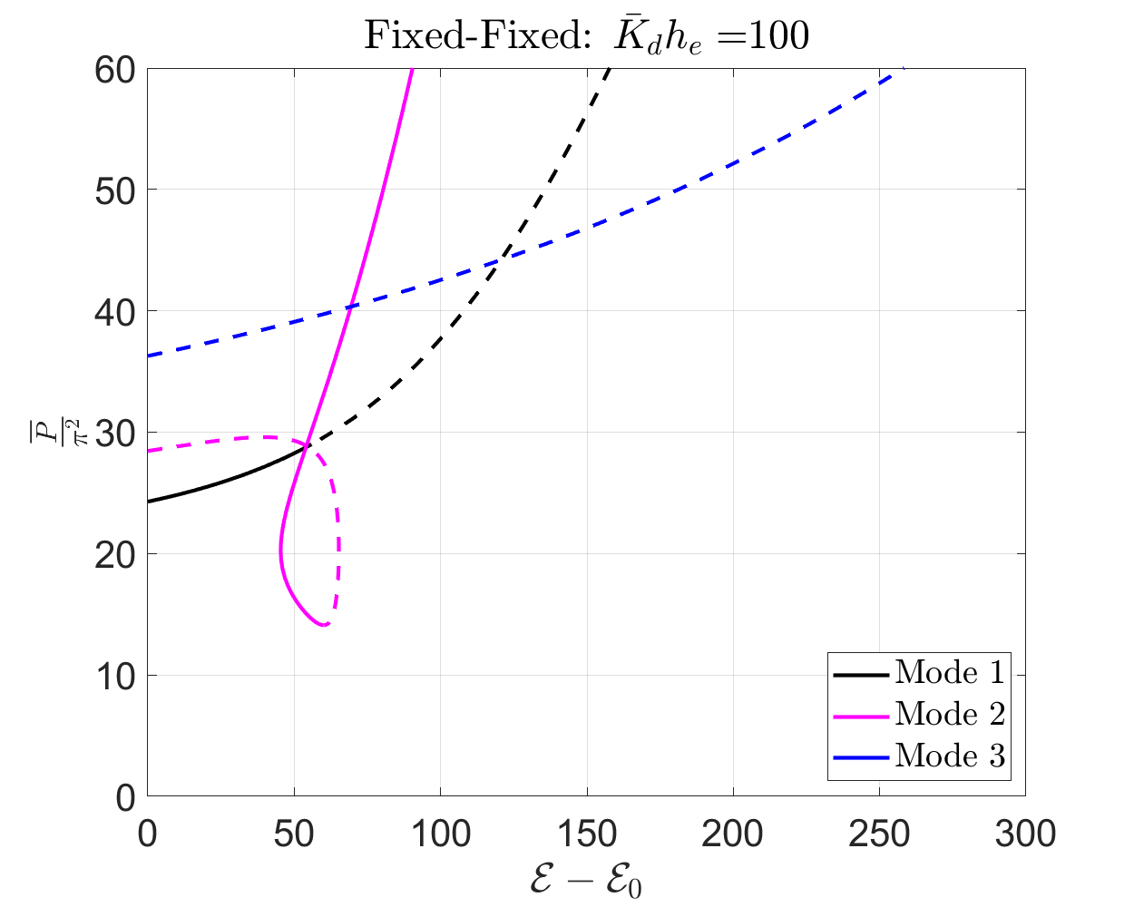
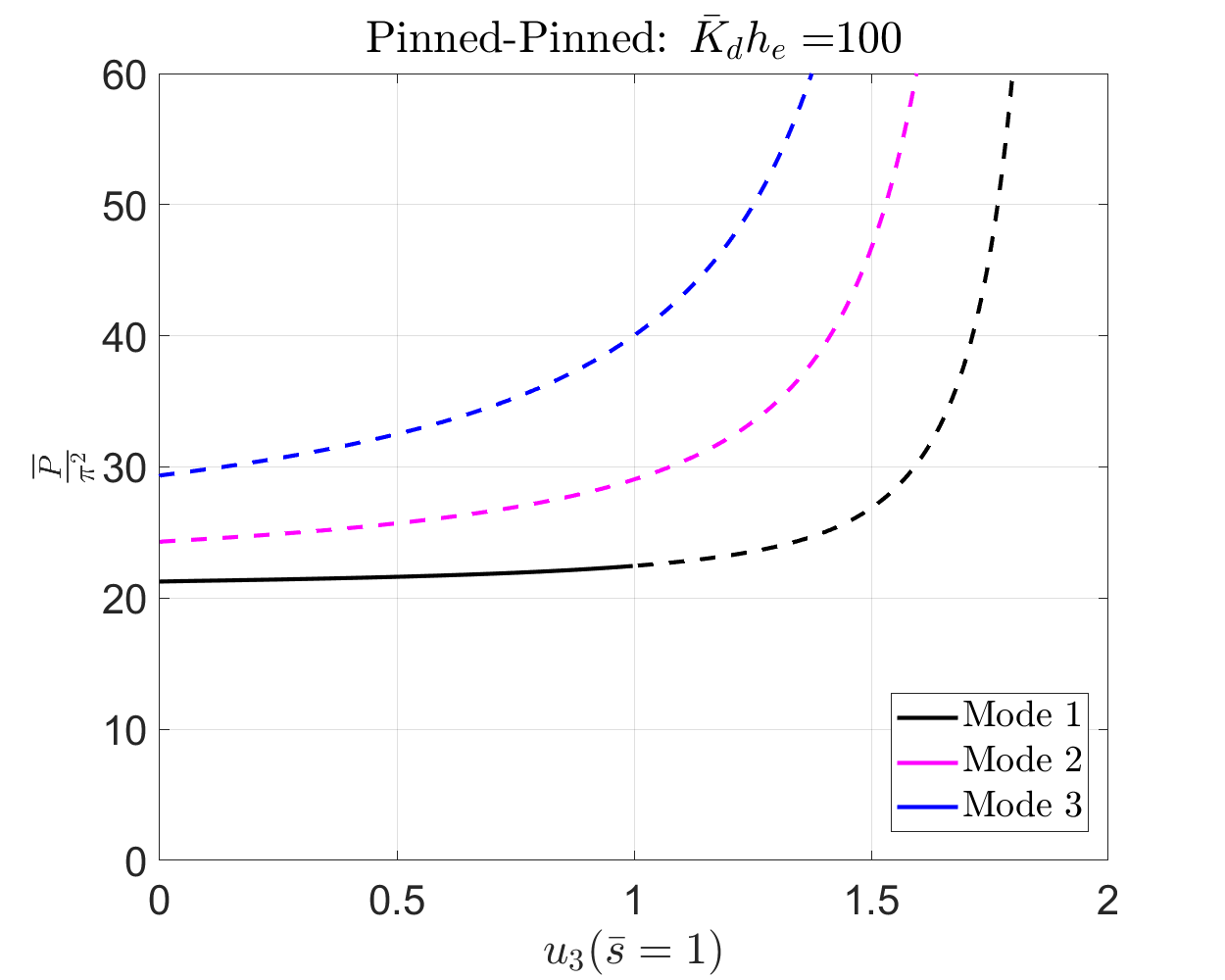
Critical buckling load is determined to be tensile under all canonical boundary conditions. Refer to Figs. 10, 11 and 12.

\bullet 

Fixed-fixed boundary conditions reveal the emergence of novel stable curves on the mode-2 branch. In Fig. 11(a), we highlight the segment of the mode-2 branch that corresponds to novel stable configurations, observed in a ferromagnetic ribbon but absent in Euler’s Elastica. A novel stable mode shape featuring two self-intersection points is shown in red in Fig. 11 (a), and additional illustrations can be found in Fig. 11 (b).

Case 2: Hard ferromagnetic ribbon:

\bullet 

Introduction of magnetization leads to an increase in the compressive buckling load compared to the Elastica. See Figs.13, 14 and 15.

\bullet 

Comparing the deformed configuration of the hard ferromagnetic ribbon to Euler’s Elastica, no discernible difference in shape is observed, despite the presence of a change in the vertical reaction force at the supports. The expressions for the vertical reaction forces at the supports are provided in Equations 75 and 76.

1.1 Organisation of the paper

The paper is organised as follows: In Section 2, we present the mathematical model for the ferromagnetic planar ribbon. Beginning with the geometry and kinematics, we then derive the total energy of soft and hard ferromagnetic planar ribbons. We conclude this section with the derivation of the equilibrium equations for various canonical boundary conditions. In Section 3, we describe the numerical continuation method employed for solving the equilibrium equations. Section 4, focuses on the stability analysis of the solutions to the equilibrium equations. Section 5 details the numerical solutions for various canonical loading scenarios. We comprehensively analyse the deformation behaviour and bifurcation patterns for various canonical loading scenarios. The end of Section 5 is devoted to a discussion in the limit as Kd¯¯subscript𝐾𝑑\bar{K_{d}} approaches infinity. Here, Kd¯¯subscript𝐾𝑑\bar{K_{d}} represents the ratio of the magnetostatic energy density to the elastic energy density of the ferromagnetic ribbon. We close our paper with the conclusions and remarks in Section 6.

2 One-dimensional model for a ferromagnetic ribbon

2.1 Kinematics of ribbons

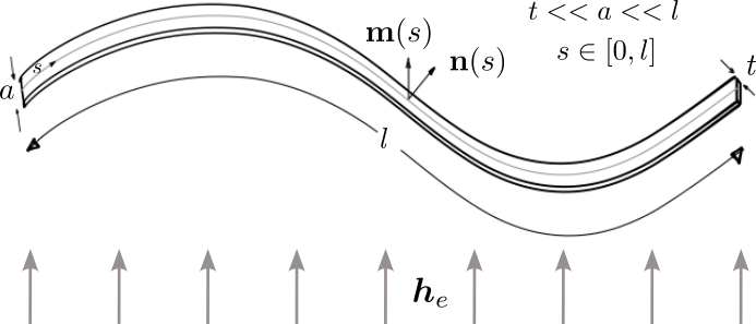
Ribbons are characterized by three disparate length scales – length (l𝑙l), width (a𝑎a), thickness (t𝑡t) – such that talmuch-less-than𝑡𝑎much-less-than𝑙t\ll a\ll l. Geometrically, ribbon is described in terms of a three-coordinate set – centerline arc length (s𝑠s), lateral (a~~𝑎\tilde{a}), transverse (t~~𝑡\tilde{t}) coordinates. In the reference configuration, the ribbon is represented in standard basis of (𝒆1,𝒆2,𝒆3)subscript𝒆1subscript𝒆2subscript𝒆3({\bf\it e}_{1},{\bf\it e}_{2},{\bf\it e}_{3}) as s𝒆3+a~𝒆1+t~𝒆2𝑠subscript𝒆3~𝑎subscript𝒆1~𝑡subscript𝒆2s{\bf\it e}_{3}+\tilde{a}{\bf\it e}_{1}+\tilde{t}{\bf\it e}_{2}. We assume that the centreline of the ribbon lies in the 𝒆2𝒆3subscript𝒆2subscript𝒆3{\bf\it e}_{2}-{\bf\it e}_{3} plane without undergoing any twist in the deformed configuration. The centreline representation of the deformed planar ribbon is given by

𝒙(s,a~,t~)𝒙𝑠~𝑎~𝑡\displaystyle{\bf\it x}(s,\tilde{a},\tilde{t}) =𝒓(s)+a~𝒅1(s)+t~𝒅2(s).absent𝒓𝑠~𝑎subscript𝒅1𝑠~𝑡subscript𝒅2𝑠\displaystyle={\bf\it r}(s)+\tilde{a}{\bf\it d}_{1}(s)+\tilde{t}{\bf\it d}_{2}(s). (1)

Here, 𝒓(s)𝒓𝑠{\bf\it r}(s) denotes the position vector of a centreline material point, (𝒅1(s),𝒅2(s),𝒅3(s))subscript𝒅1𝑠subscript𝒅2𝑠subscript𝒅3𝑠({\bf\it d}_{1}(s),{\bf\it d}_{2}(s),{\bf\it d}_{3}(s)) is the orthonormal material frame basis, and s[0,l],a~[a2,a2],t~[t2,t2]formulae-sequence𝑠0𝑙formulae-sequence~𝑎𝑎2𝑎2~𝑡𝑡2𝑡2s\in[0,l],\leavevmode\nobreak\ \tilde{a}\in\left[-\frac{a}{2},\frac{a}{2}\right],\leavevmode\nobreak\ \tilde{t}\in\left[-\frac{t}{2},\frac{t}{2}\right]. The ribbon is assumed to be inextensible, uniform and obeys Kirchhoff’s hypothesis, that is, normal sections to the centreline remain normal after deformation Bigoni2015 . The condition of inextensibility implies d𝒓ds(s)=𝒅3(s)derivative𝑠𝒓𝑠subscript𝒅3𝑠\derivative{{\bf\it r}}{s}(s)={\bf\it d}_{3}(s). Also, since the ribbon does not twist, we have 𝒅1(s)=𝒆1subscript𝒅1𝑠subscript𝒆1{\bf\it d}_{1}(s)={\bf\it e}_{1}.

Refer to caption
Figure 2: Geometry of the ferromagnetic ribbon illustrating the representation of magnetisation vector 𝒎(s)𝒎𝑠{\bf\it m}(s) and normal vector 𝒏(s)𝒏𝑠{\bf\it n}(s) = 𝒅2(s)subscript𝒅2𝑠{\bf\it d}_{2}(s).

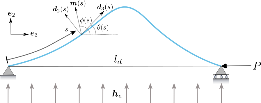
The schematic of the centerline in the deformed configuration is shown in Fig. 3 and the coordinates of the centerline in (𝒆1,𝒆2,𝒆3)subscript𝒆1subscript𝒆2subscript𝒆3({\bf\it e}_{1},{\bf\it e}_{2},{\bf\it e}_{3}) basis is given as follows:

x(s)𝑥𝑠\displaystyle x(s) =0,absent0\displaystyle=0, (2)
y(s)𝑦𝑠\displaystyle y(s) =0ssinθ(t)𝑑t,absentsuperscriptsubscript0𝑠𝜃𝑡differential-d𝑡\displaystyle=\int_{0}^{s}\sin\theta(t)\leavevmode\nobreak\ dt, (3)
z(s)𝑧𝑠\displaystyle z(s) =0scosθ(t)𝑑t,absentsuperscriptsubscript0𝑠𝜃𝑡differential-d𝑡\displaystyle=\int_{0}^{s}\cos\theta(t)\leavevmode\nobreak\ dt, (4)

where s𝑠s denotes arc length coordinate, θ(s)𝜃𝑠\theta(s) is the angle between 𝒅3(s)subscript𝒅3𝑠{\bf\it d}_{3}(s) and 𝒆3subscript𝒆3{\bf\it e}_{3} basis vector at s𝑠s.

Refer to caption
Figure 3: Schematic setup of the ferromagnetic ribbon.

2.2 Energy formulation

The free energy functional of ferromagnetic ribbon is equal to the sum of its magnetic energy, elastic energy and the loading device energy. We will assume that the primary source of the magnetic energy arises from the demag. energy and Zeeman energy.

Given our assumption that the ribbon is made of an inextensible ferromagnetic material, the primary source of the elastic energy is the bending energy. We denote the sum of the bending energy and the loading device energy as elasticasubscriptelastica\mathcal{E}_{\text{elastica}} which is given as follows:

elasticasubscriptelastica\displaystyle\mathcal{E}_{\text{elastica}} =120lEIκ2(s)𝑑sElastic (or bending) energy+P(10lcosθ(s)ds),Loading energy\displaystyle=\underbrace{\frac{1}{2}\int_{0}^{l}EI\kappa^{2}(s)ds}_{\text{Elastic (or bending) energy}}+\underbrace{P\left(1-\int_{0}^{l}\cos\theta(s)ds\right),}_{\text{Loading energy}} (5)

subject to the integral constraint

y(l)=0lsinθ(s)𝑑s=0.𝑦𝑙superscriptsubscript0𝑙𝜃𝑠differential-d𝑠0\begin{split}y(l)=\int_{0}^{l}\sin\theta(s)\leavevmode\nobreak\ ds=0.\end{split} (6)

Here, κ(s)=dθ(s)ds𝜅𝑠derivative𝑠𝜃𝑠\kappa(s)=\derivative{\theta(s)}{s} is the bending curvature, E𝐸E is the Young’s modulus, I=at312𝐼𝑎superscript𝑡312I=\frac{at^{3}}{12} is the area moment of inertia (EI𝐸𝐼EI is the bending stiffness of the cross section), and P𝑃P is the horizontal load.

We now proceed to write down the magnetic energy of the ribbon. We employ the theoretical framework of micromagnetics to formulate the magnetic energy associated with a ferromagnetic ribbon. Recall that the magnetisation vector: 𝒎(𝒙)𝒎𝒙{\bf\it m}({\bf\it x}), is the primary variable in the micromagnetics functional. The magnetisation vector 𝒎(𝒙)𝒎𝒙{\bf\it m}({\bf\it x}) is supported on ΩΩ\Omega and |𝒎(𝒙)|=1,𝒙Ωformulae-sequence𝒎𝒙1𝒙Ω|{\bf\it m}({\bf\it x})|=1,{\bf\it x}\in\Omega. In our analysis, ΩΩ\Omega represents the deformed planar ferromagnetic ribbon. We now examine the various terms of the micromagnetic functional when applied to our ferromagnetic ribbon. For a detailed exposition on the micromagnetic functional, we refer the reader to dabade2019micromagnetics .

The exchange energy penalizes the gradient of the magnetisation and is expressed as follows:

ex=AΩ|𝒎(𝒙)|2𝑑𝒙,subscript𝑒𝑥𝐴subscriptΩsuperscript𝒎𝒙2differential-d𝒙\displaystyle\mathcal{E}_{ex}=A\int_{\Omega}\absolutevalue{\nabla{{\bf\it m}({\bf\it x})}}^{2}d{\bf\it x}, (7)

where A𝐴A is a material parameter known as the exchange constant. The exchange energy constrains the magnetisation to vary exclusively along the arc length parameter s𝑠s. If the magnetisation varies across the width and thickness of the sample, the exchange energy per unit volume scales as 𝒪(Aw2)𝒪𝐴superscript𝑤2\mathcal{O}\big{(}\frac{A}{w^{2}}\big{)} and 𝒪(At2)𝒪𝐴superscript𝑡2\mathcal{O}\big{(}\frac{A}{t^{2}}\big{)}, respectively. The small values of t𝑡t and w𝑤w, that is t<w<<A𝑡𝑤much-less-than𝐴t<w<<\sqrt{A}, prevent spatial variation in magnetisation across the width and thickness. Consequently, we assume that magnetisation only varies along the length of the ribbon, i.e., 𝒎(𝒙)=𝒎(s)𝒎𝒙𝒎𝑠{\bf\it m}({\bf\it x})={\bf\it m}({s}). Further, we shall assume that l>>Amuch-greater-than𝑙𝐴l>>\sqrt{A}, such that Al2<<1much-less-than𝐴superscript𝑙21\frac{A}{l^{2}}<<1, and hence we can ignore the exchange energy per unit volume if 𝒎(𝒙)=𝒎(s)𝒎𝒙𝒎𝑠{\bf\it m}({\bf\it x})={\bf\it m}({s}).

The magnetocrystalline anisotropy energy governs the favored orientations for the magnetisation vector within the ferromagnetic sample. It is quantified by the material parameter Kasubscript𝐾𝑎K_{a}, known as the anisotropy constant. In Case 1. (soft ferromagnet), Ka<<1much-less-thansubscript𝐾𝑎1K_{a}<<1 and the magnetocrystalline anisotropy energy is very small, and the magnetisation has no preferred direction of orientation. Whereas, in Case 2. (hard ferromagnet), Ka>>1much-greater-thansubscript𝐾𝑎1K_{a}>>1 the magnetocrystalline anisotropy energy is very large and and the magnetisation vector makes a fixed angle with tangent along the length of the ribbon.

We now write down the demag. energy of the planar ribbon. The demag. energy associated with planar ribbon is computed by solving Maxwell’s equations of magnetostatics, namely,

×𝒉m(𝒙)subscript𝒉𝑚𝒙\displaystyle\curl{{\bf\it h}_{m}({\bf\it x})} =0,absentbold-italic-0\displaystyle={\bf\it 0}, (8)
(𝒉m(𝒙)+𝒎(𝒙))subscript𝒉𝑚𝒙𝒎𝒙\displaystyle\divergence({\bf\it h}_{m}({\bf\it x})+{\bf\it m}({\bf\it x})) =0.absent0\displaystyle=0. (9)

Here, 𝒎(𝒙)𝒎𝒙{\bf\it m}({\bf\it x}) is the magnetisation vector defined on the ferromagnetic body and is equal to zero outside the body. The field induced due to the magnetisation 𝒎(𝒙)𝒎𝒙{\bf\it m}({\bf\it x}) is denoted by 𝒉m(𝒙)subscript𝒉𝑚𝒙{\bf\it h}_{m}({\bf\it x}). The induced magnetic field 𝒉m(𝒙)subscript𝒉𝑚𝒙{\bf\it h}_{m}({\bf\it x}) can be found by solving Maxwell’s equations of magnetostatics.

The demag. energy is evaluated by computing the square of the L2superscript𝐿2L^{2}-norm of 𝒉m(𝒙)subscript𝒉𝑚𝒙{\bf\it h}_{m}({\bf\it x}) on all of 3superscript3\mathbb{R}^{3}, it can be conveniently calculated in terms of Fourier transform of 𝒎(𝒙)𝒎𝒙{\bf\it m}({\bf\it x}), as follows 111Details of this calculation and other computations involved in this section can be found in appendix A.

demag.=Kd2|𝒉m|2𝑑𝒙subscriptdemag.subscript𝐾𝑑subscriptsuperscript2superscriptsubscript𝒉𝑚2differential-d𝒙\displaystyle\mathcal{E}_{\text{demag.}}=K_{d}\int_{\mathbb{R}^{2}}\absolutevalue{{\bf\it h}_{m}}^{2}\leavevmode\nobreak\ d{\bf\it x} =Kd3|𝒎^(𝝃)|2|𝝃|2𝑑𝝃,absentsubscript𝐾𝑑subscriptsuperscript3superscript^𝒎𝝃2superscript𝝃2differential-d𝝃\displaystyle=K_{d}\int_{\mathbb{R}^{3}}\frac{\absolutevalue{\widehat{\divergence{{\bf\it m}}}({\bf\it\xi})}^{2}}{\absolutevalue{{\bf\it\xi}}^{2}}d{\bf\it\xi}, (10)

where Kd=Ms22μ0subscript𝐾𝑑superscriptsubscript𝑀𝑠22subscript𝜇0K_{d}=\frac{M_{s}^{2}}{2\mu_{0}} is the magnetostatic energy constant, Mssubscript𝑀𝑠M_{s} is the saturation magnetization of the material, and μ0subscript𝜇0\mu_{0} is the permeability of the free space.

We carry out the above integration in the material frame (𝒅1(s),𝒅2(s),𝒅3(s))subscript𝒅1𝑠subscript𝒅2𝑠subscript𝒅3𝑠({\bf\it d}_{1}(s),{\bf\it d}_{2}(s),{\bf\it d}_{3}(s)). In the material frame, 𝒙𝒓(s)+a~𝒅1(s)+t~𝒅2(s)maps-to𝒙𝒓𝑠~𝑎subscript𝒅1𝑠~𝑡subscript𝒅2𝑠{\bf\it x}\mapsto{\bf\it r}(s)+\tilde{a}{\bf\it d}_{1}(s)+\tilde{t}{\bf\it d}_{2}(s), and s[0,l],a~[a2,a2],t~[t2,t2]formulae-sequence𝑠0𝑙formulae-sequence~𝑎𝑎2𝑎2~𝑡𝑡2𝑡2s\in[0,l],\leavevmode\nobreak\ \tilde{a}\in\left[-\frac{a}{2},\frac{a}{2}\right],\leavevmode\nobreak\ \tilde{t}\in\left[-\frac{t}{2},\frac{t}{2}\right], and 𝒓(s)=𝒅3(s)superscript𝒓𝑠subscript𝒅3𝑠{\bf\it r}^{\prime}(s)={\bf\it d}_{3}(s). The Fourier transform of 𝒎𝒎{\bf\it m} in the material frame as follows:

𝒎^(𝝃)^𝒎𝝃\displaystyle\widehat{\divergence{{\bf\it m}}}({\bf\it\xi}) =(𝒎)exp(i2π𝒙𝝃)𝑑𝒙absent𝒎𝑖2𝜋𝒙𝝃differential-d𝒙\displaystyle=\int(\divergence{{\bf\it m}})\exp(-i2\pi{\bf\it x}\cdot{\bf\it\xi})d{\bf\it x} (11)
=1J(a~md1+t~+κ[t~a~md1+t~t~md2+md2])exp(i2π(sξd3+a~ξd1+t~ξd2))J𝑑s𝑑a~𝑑t~.absent1𝐽subscript~𝑎subscript𝑚subscript𝑑1subscript~𝑡𝜅delimited-[]~𝑡subscript~𝑎subscript𝑚subscript𝑑1~𝑡subscript~𝑡subscript𝑚subscript𝑑2subscript𝑚subscript𝑑2𝑖2𝜋𝑠subscript𝜉subscript𝑑3~𝑎subscript𝜉subscript𝑑1~𝑡subscript𝜉subscript𝑑2𝐽differential-d𝑠differential-d~𝑎differential-d~𝑡\displaystyle=\int\frac{1}{J}\left(\partial_{\tilde{a}}m_{d_{1}}+\partial_{\tilde{t}}+\kappa[\tilde{t}\partial_{\tilde{a}}m_{d_{1}}+\tilde{t}\partial_{\tilde{t}}m_{d_{2}}+m_{d_{2}}]\right)\exp(-i2\pi(s\xi_{d_{3}}+\tilde{a}\xi_{d_{1}}+\tilde{t}\xi_{d_{2}}))Jdsd\tilde{a}d\tilde{t}. (12)

Here, J𝐽J is the Jacobian involved in computing the divergence of 𝒎𝒎{\bf\it m} and in the change of variables from (x1,x2,x3)subscript𝑥1subscript𝑥2subscript𝑥3(x_{1},x_{2},x_{3}) to (s,a~,t~)𝑠~𝑎~𝑡(s,\tilde{a},\tilde{t}). Furthermore, mdi=𝒎𝒅i(s),ξdi=𝝃𝒅i(s)formulae-sequencesubscript𝑚subscript𝑑𝑖𝒎subscript𝒅𝑖𝑠subscript𝜉subscript𝑑𝑖𝝃subscript𝒅𝑖𝑠m_{d_{i}}={\bf\it m}\cdot{\bf\it d}_{i}(s),\leavevmode\nobreak\ \xi_{d_{i}}={\bf\it\xi}\cdot{\bf\it d}_{i}(s).

Since the ribbon under study is narrow, we shall assume 𝒎(𝒙)=𝒎(s)𝒎𝒙𝒎𝑠{\bf\it m}({\bf\it x})={\bf\it m}(s) and in the above computation, the magnetostatic or demag. energy simplifies as follows:

demag.=Kd3|𝒎^(𝝃)|2|𝝃|2𝑑𝝃=Kd3|𝒎^(ξd1,ξd2,ξd3)|2ξd12+ξd22+ξd32𝑑ξd1𝑑ξd2𝑑ξd3=Kdat|md3^(ξd2)|2𝑑ξd3+𝒪(t2)=Kdats=0l(md2)2𝑑s+𝒪(t2)=Kdat0l(𝒎𝒅2)2𝑑s+𝒪(t2).subscriptdemag.subscript𝐾𝑑subscriptsuperscript3superscript^𝒎𝝃2superscript𝝃2differential-d𝝃subscript𝐾𝑑subscriptsuperscript3superscript^𝒎subscript𝜉subscript𝑑1subscript𝜉subscript𝑑2subscript𝜉subscript𝑑32superscriptsubscript𝜉subscript𝑑12superscriptsubscript𝜉subscript𝑑22superscriptsubscript𝜉subscript𝑑32differential-dsubscript𝜉subscript𝑑1differential-dsubscript𝜉subscript𝑑2differential-dsubscript𝜉subscript𝑑3subscript𝐾𝑑𝑎𝑡subscriptsuperscript^subscript𝑚subscript𝑑3subscript𝜉subscript𝑑22differential-dsubscript𝜉subscript𝑑3𝒪superscript𝑡2subscript𝐾𝑑𝑎𝑡superscriptsubscript𝑠0𝑙superscriptsubscript𝑚subscript𝑑22differential-d𝑠𝒪superscript𝑡2subscript𝐾𝑑𝑎𝑡superscriptsubscript0𝑙superscript𝒎subscript𝒅22differential-d𝑠𝒪superscript𝑡2\begin{split}\mathcal{E}_{\text{demag.}}=K_{d}\int_{\mathbb{R}^{3}}\frac{\absolutevalue{\widehat{\divergence{{\bf\it m}}}({\bf\it\xi})}^{2}}{\absolutevalue{{\bf\it\xi}}^{2}}d{\bf\it\xi}&=K_{d}\int_{\mathbb{R}^{3}}\frac{\absolutevalue{\widehat{\divergence{{\bf\it m}}}(\xi_{d_{1}},\xi_{d_{2}},\xi_{d_{3}})}^{2}}{\xi_{d_{1}}^{2}+\xi_{d_{2}}^{2}+\xi_{d_{3}}^{2}}d\xi_{d_{1}}d\xi_{d_{2}}d\xi_{d_{3}}\\ &=K_{d}at\int_{\mathbb{R}}\absolutevalue{\widehat{m_{d_{3}}}(\xi_{d_{2}})}^{2}d\xi_{d_{3}}+\mathcal{O}(t^{2})\\ &=K_{d}at\int_{s=0}^{l}(m_{d_{2}})^{2}ds+\mathcal{O}(t^{2})\\ &=K_{d}at\int_{0}^{l}({\bf\it m}\cdot{\bf\it d}_{2})^{2}ds+\mathcal{O}(t^{2}).\end{split} (13)

The Zeeman energy of the ribbon due to external magnetic field 𝒉esubscript𝒉𝑒{\bf\it h}_{e} is

Zeeman=2Kdat0l𝒉e𝒎𝑑s.subscriptZeeman2subscript𝐾𝑑𝑎𝑡superscriptsubscript0𝑙subscript𝒉𝑒𝒎differential-d𝑠\mathcal{E}_{\text{Zeeman}}=-2K_{d}at\int_{0}^{l}{\bf\it h}_{e}\cdot{\bf\it m}ds. (14)

In this paper, we shall only consider the leading order magnetostatic energy and hence our total magnetic energy is

magnetic=demag.+Zeeman=Kdat0l(𝒎𝒅2)2𝑑s2Kdat0l𝒉e𝒎𝑑s.subscriptmagneticsubscriptdemag.subscriptZeemansubscript𝐾𝑑𝑎𝑡superscriptsubscript0𝑙superscript𝒎subscript𝒅22differential-d𝑠2subscript𝐾𝑑𝑎𝑡superscriptsubscript0𝑙subscript𝒉𝑒𝒎differential-d𝑠\mathcal{E}_{\text{magnetic}}=\mathcal{E}_{\text{demag.}}+\mathcal{E}_{\text{Zeeman}}=K_{d}at\int_{0}^{l}({\bf\it m}\cdot{\bf\it d}_{2})^{2}ds-2K_{d}at\int_{0}^{l}{\bf\it h}_{e}\cdot{\bf\it m}ds. (15)

Therefore, the total energy is the sum of magneticsubscriptmagnetic\mathcal{E}_{\text{magnetic}} (Eqn. (15)) and elasticasubscriptelastica\mathcal{E}_{\text{elastica}} (Eqn. (5)) and is given as follows:

(θ,𝒎)𝜃𝒎\displaystyle\mathcal{E}(\theta,{\bf\it m}) =120lEIκ2(s)𝑑s+P(10lcosθ(s)𝑑s)+Kdat0l(𝒎𝒅2)2𝑑s2Kdat0l𝒉e𝒎𝑑s.absent12superscriptsubscript0𝑙𝐸𝐼superscript𝜅2𝑠differential-d𝑠𝑃1superscriptsubscript0𝑙𝜃𝑠differential-d𝑠subscript𝐾𝑑𝑎𝑡superscriptsubscript0𝑙superscript𝒎subscript𝒅22differential-d𝑠2subscript𝐾𝑑𝑎𝑡superscriptsubscript0𝑙subscript𝒉𝑒𝒎differential-d𝑠\displaystyle=\frac{1}{2}\int_{0}^{l}EI\kappa^{2}(s)ds+P\left(1-\int_{0}^{l}\cos\theta(s)ds\right)+K_{d}at\int_{0}^{l}({\bf\it m}\cdot{\bf\it d}_{2})^{2}ds-2K_{d}at\int_{0}^{l}{\bf\it h}_{e}\cdot{\bf\it m}ds. (16)

2.3 Planar deformation of magnetoelastic ribbons

Incorporating the integral constraint (Eqn. 6), the augmented energy functional for magnetoelastic ribbon, here, ferromagnetic ribbon, is expressed as

(θ,𝒎)=120lEIκ2(s)𝑑s+P(10lcosθ(s)𝑑s)+Kdat0l(𝒎𝒅2)2𝑑s2Kdat0l𝒉e𝒎𝑑sR0lsinθ(s)𝑑s𝜃𝒎12superscriptsubscript0𝑙𝐸𝐼superscript𝜅2𝑠differential-d𝑠𝑃1superscriptsubscript0𝑙𝜃𝑠differential-d𝑠subscript𝐾𝑑𝑎𝑡superscriptsubscript0𝑙superscript𝒎subscript𝒅22differential-d𝑠2subscript𝐾𝑑𝑎𝑡superscriptsubscript0𝑙subscript𝒉𝑒𝒎differential-d𝑠𝑅superscriptsubscript0𝑙𝜃𝑠differential-d𝑠\mathcal{E}(\theta,{\bf\it m})=\frac{1}{2}\int_{0}^{l}EI\kappa^{2}(s)ds+P\left(1-\int_{0}^{l}\cos\theta(s)ds\right)+K_{d}at\int_{0}^{l}({\bf\it m}\cdot{\bf\it d}_{2})^{2}ds\\ -2K_{d}at\int_{0}^{l}{\bf\it h}_{e}\cdot{\bf\it m}ds-R\int_{0}^{l}\sin\theta(s)ds (17)

The tangent vector field 𝒅3(s)subscript𝒅3𝑠{\bf\it d}_{3}(s) (or 𝒕(s)𝒕𝑠{\bf\it t}(s)) is 𝒅3(s)=(0,sinθ(s),cosθ(s))subscript𝒅3𝑠0𝜃𝑠𝜃𝑠{\bf\it d}_{3}(s)=(0,\sin\theta(s),\cos\theta(s)) and so the normal vector field Pressley2010 is 𝒅2(s)=d𝒕ds/|d𝒕ds|=(0,cosθ(s),sinθ(s))subscript𝒅2𝑠derivative𝑠𝒕derivative𝑠𝒕0𝜃𝑠𝜃𝑠{\bf\it d}_{2}(s)=\derivative{{\bf\it t}}{s}/\absolutevalue{\derivative{{\bf\it t}}{s}}=(0,\cos\theta(s),-\sin\theta(s)). Since |𝒎(s)|=1𝒎𝑠1\absolutevalue{{\bf\it m}(s)}=1, we can write 𝒎=(0,sinϕ(s),cosϕ(s))𝒎0italic-ϕ𝑠italic-ϕ𝑠{\bf\it m}=(0,\sin\phi(s),\cos\phi(s)), ϕ(s)italic-ϕ𝑠\phi(s) is the angle between 𝒎(s)𝒎𝑠{\bf\it m}(s) and 𝒆3subscript𝒆3{\bf\it e}_{3} at s𝑠s. Similarly, external magnetic field can be represented as 𝒉e=he(0,sinψ,cosψ)subscript𝒉𝑒subscript𝑒0𝜓𝜓{\bf\it h}_{e}=h_{e}(0,\sin\psi,\cos\psi), where ψ𝜓\psi is the angle between 𝒉esubscript𝒉𝑒{\bf\it h}_{e} and 𝒆3subscript𝒆3{\bf\it e}_{3}, and hesubscript𝑒\it{h_{e}} is the strength of the externally applied magnetic field. Substituting the expressions for 𝒎𝒎{\bf\it m} and 𝒉esubscript𝒉𝑒{\bf\it h}_{e} into Eqn. 17 leads to

(θ,ϕ)𝜃italic-ϕ\displaystyle\mathcal{E}(\theta,\phi) =EI20l(θ(s))2𝑑s+Kdat0l(sinθcosϕ+cosθsinϕ)2𝑑s2Kdathe0l(cosψcosϕ+sinψsinϕ)𝑑sabsent𝐸𝐼2superscriptsubscript0𝑙superscriptsuperscript𝜃𝑠2differential-d𝑠subscript𝐾𝑑𝑎𝑡superscriptsubscript0𝑙superscript𝜃italic-ϕ𝜃italic-ϕ2differential-d𝑠2subscript𝐾𝑑𝑎𝑡subscript𝑒superscriptsubscript0𝑙𝜓italic-ϕ𝜓italic-ϕdifferential-d𝑠\displaystyle=\frac{EI}{2}\int_{0}^{l}(\theta^{\prime}(s))^{2}ds+K_{d}at\int_{0}^{l}(-\sin\theta\cos\phi+\cos\theta\sin\phi)^{2}ds-2K_{d}ath_{e}\int_{0}^{l}(\cos\psi\cos\phi+\sin\psi\sin\phi)ds
P(10lcosθ(s)𝑑s)R0lsinθ(s)𝑑s𝑃1superscriptsubscript0𝑙𝜃𝑠differential-d𝑠𝑅superscriptsubscript0𝑙𝜃𝑠differential-d𝑠\displaystyle\qquad-P\bigg{(}1-\int_{0}^{l}\cos\theta(s)ds\bigg{)}-R\int_{0}^{l}\sin\theta(s)ds
=EI20l(θ(s))2𝑑s+Kdat0lsin2(ϕθ)𝑑s2Kdathe0lcos(ϕψ)𝑑sabsent𝐸𝐼2superscriptsubscript0𝑙superscriptsuperscript𝜃𝑠2differential-d𝑠subscript𝐾𝑑𝑎𝑡superscriptsubscript0𝑙superscript2italic-ϕ𝜃differential-d𝑠2subscript𝐾𝑑𝑎𝑡subscript𝑒superscriptsubscript0𝑙italic-ϕ𝜓differential-d𝑠\displaystyle=\frac{EI}{2}\int_{0}^{l}(\theta^{\prime}(s))^{2}ds+K_{d}at\int_{0}^{l}\sin^{2}(\phi-\theta)ds-2K_{d}ath_{e}\int_{0}^{l}\cos(\phi-\psi)ds
P(10lcosθ(s)𝑑s)R0lsinθ(s)𝑑s.𝑃1superscriptsubscript0𝑙𝜃𝑠differential-d𝑠𝑅superscriptsubscript0𝑙𝜃𝑠differential-d𝑠\displaystyle\qquad-P\bigg{(}1-\int_{0}^{l}\cos\theta(s)ds\bigg{)}-R\int_{0}^{l}\sin\theta(s)ds. (18)

We use a non-dimensional arc length parameter defined as s¯:=sLassign¯𝑠𝑠𝐿\bar{s}:=\frac{s}{L} and define Θ(s¯)Θ¯𝑠\Theta(\bar{s}) and Φ(s¯)Φ¯𝑠\Phi(\bar{s}) as follows:

Θ(s¯)=θ(s(s¯)),Φ(s¯)=ϕ(s(s¯)).formulae-sequenceΘ¯𝑠𝜃𝑠¯𝑠Φ¯𝑠italic-ϕ𝑠¯𝑠\Theta(\bar{s})=\theta(s(\bar{s})),\quad\Phi(\bar{s})=\phi(s(\bar{s})). (19)

The augmented energy functional is also non-dimensionalized as follows:

¯(Θ,Φ)=(Θ,Φ)EI/l¯ΘΦΘΦ𝐸𝐼𝑙\displaystyle\bar{\mathcal{E}}(\Theta,\Phi)=\frac{\mathcal{E}(\Theta,\Phi)}{EI/l} =1201(Θ(s¯))2𝑑s¯+K¯d01sin2(Φ(s¯)Θ(s¯))𝑑s¯2K¯dhe01cos(Φ(s¯)ψ)𝑑s¯absent12superscriptsubscript01superscriptsuperscriptΘ¯𝑠2differential-d¯𝑠subscript¯𝐾𝑑superscriptsubscript01superscript2Φ¯𝑠Θ¯𝑠differential-d¯𝑠2subscript¯𝐾𝑑subscript𝑒superscriptsubscript01Φ¯𝑠𝜓differential-d¯𝑠\displaystyle=\frac{1}{2}\int_{0}^{1}(\Theta^{\prime}(\bar{s}))^{2}d\bar{s}+\bar{K}_{d}\int_{0}^{1}\sin^{2}(\Phi(\bar{s})-\Theta(\bar{s}))d\bar{s}-2\bar{K}_{d}h_{e}\int_{0}^{1}\cos(\Phi(\bar{s})-\psi)d\bar{s}
P¯(101cosΘ(s¯)𝑑s¯)R¯01sinΘ(s¯)𝑑s¯,¯𝑃1superscriptsubscript01Θ¯𝑠differential-d¯𝑠¯𝑅superscriptsubscript01Θ¯𝑠differential-d¯𝑠\displaystyle\qquad-\bar{P}\bigg{(}1-\int_{0}^{1}\cos\Theta(\bar{s})d\bar{s}\bigg{)}-\bar{R}\int_{0}^{1}\sin\Theta(\bar{s})d\bar{s}, (20)

where, K¯dsubscript¯𝐾𝑑\bar{K}_{d}, P¯¯𝑃\bar{P} and Q¯¯𝑄\bar{Q} are non-dimensional numbers defined as follows:

K¯d=Kdatl2EI=12KdE(lt)2,P¯=Pl2EI andR¯=Rl2EI.formulae-sequencesubscript¯𝐾𝑑subscript𝐾𝑑𝑎𝑡superscript𝑙2𝐸𝐼12subscript𝐾𝑑𝐸superscript𝑙𝑡2formulae-sequence¯𝑃𝑃superscript𝑙2𝐸𝐼 and¯𝑅𝑅superscript𝑙2𝐸𝐼\bar{K}_{d}=\frac{K_{d}atl^{2}}{EI}=\frac{12K_{d}}{E}\left(\frac{l}{t}\right)^{2},\quad\bar{P}=\frac{Pl^{2}}{EI}\text{ and}\quad\bar{R}=\frac{Rl^{2}}{EI}.

Note that K¯dsubscript¯𝐾𝑑\bar{K}_{d} is an important non-dimensional number in our analysis and represents the ratio of the demag. energy and the elastic energy of the ferromagnetic ribbon It depends on the material properties and the aspect ratio (tl𝑡𝑙\frac{t}{l}) of the ferromagnetic ribbon. Henceforth, for simplification, we replace ΘΘ\Theta and ΦΦ\Phi with θ𝜃\theta and ϕitalic-ϕ\phi, respectively. We will now tailor our energy functional for the two following scenarios: 1. soft ferromagnetic ribbon and 2. hard ferromagnetic ribbon.

2.4 Case 1. Soft ferromagnet.

A soft ferromagnet is a ferromagnet with very small magnetic anisotropy energy (Ka<<1much-less-thansubscript𝐾𝑎1K_{a}<<1), Dabade2018 . The magnetisation vector has no preferred direction of alignment within the ferromagnetic solid. Thus, the magnetisation vector rotates and aligns along the externally applied magnetic field for sufficiently large fields (Fig. 4). That is, 𝒎(s¯)𝒉econditional𝒎¯𝑠subscript𝒉𝑒{\bf\it m}(\bar{s})\parallel{\bf\it h}_{e}, and as a result, the Zeeman energy minimized and not considered in the analysis. The deformation in this case is driven by the interplay among demag. energy, bending energy, and loading device energy.

Since 𝒎(s¯)𝒉econditional𝒎¯𝑠subscript𝒉𝑒{\bf\it m}(\bar{s})\parallel{\bf\it h}_{e}, we have 𝒎(s¯)𝒉e=he𝒎¯𝑠subscript𝒉𝑒subscript𝑒{\bf\it m}(\bar{s})\cdot{\bf\it h}_{e}=h_{e} implying that ϕ(s¯)=ψitalic-ϕ¯𝑠𝜓\phi(\bar{s})=\psi. Therefore, Eqn. 20 becomes

¯(θ,ϕ)=1201(θ(s¯))2𝑑s¯+K¯d01sin2(ϕ(s¯)θ(s¯))𝑑s¯+P¯01cosθ(s¯)𝑑s¯R¯01sinθ(s¯)𝑑s¯P¯2K¯dhe.¯𝜃italic-ϕ12superscriptsubscript01superscriptsuperscript𝜃¯𝑠2differential-d¯𝑠subscript¯𝐾𝑑superscriptsubscript01superscript2italic-ϕ¯𝑠𝜃¯𝑠differential-d¯𝑠¯𝑃superscriptsubscript01𝜃¯𝑠differential-d¯𝑠¯𝑅superscriptsubscript01𝜃¯𝑠differential-d¯𝑠¯𝑃2subscript¯𝐾𝑑subscript𝑒\bar{\mathcal{E}}(\theta,\phi)=\frac{1}{2}\int_{0}^{1}(\theta^{\prime}(\bar{s}))^{2}d\bar{s}+\bar{K}_{d}\int_{0}^{1}\sin^{2}(\phi(\bar{s})-\theta(\bar{s}))d\bar{s}+\bar{P}\int_{0}^{1}\cos\theta(\bar{s})d\bar{s}-\bar{R}\int_{0}^{1}\sin\theta(\bar{s})d\bar{s}-\bar{P}-2\bar{K}_{d}h_{e}. (21)

We now proceed to derive the Euler-Lagrange equations, i.e., equilibrium equations and generic boundary conditions. Introducing first order perturbations to the unknown variables θ𝜃\theta and ϕitalic-ϕ\phi as θ~(s¯)=θ(s¯)+ϵη(s¯)~𝜃¯𝑠𝜃¯𝑠italic-ϵ𝜂¯𝑠\widetilde{\theta}(\bar{s})=\theta(\bar{s})+\epsilon\eta(\bar{s}), and putting it into Eqn. 21 gives

¯(θ~,ψ)=1201(θ(s¯)+ϵη(s¯))2𝑑s¯+K¯d01sin2(ψθ(s¯)ϵη(s¯))𝑑s¯+P¯01cos(θ(s¯)+ϵη(s¯))𝑑s¯R¯01sin(θ(s¯)+ϵη(s¯))𝑑s¯P¯2K¯dhe.¯~𝜃𝜓12superscriptsubscript01superscriptsuperscript𝜃¯𝑠italic-ϵsuperscript𝜂¯𝑠2differential-d¯𝑠subscript¯𝐾𝑑superscriptsubscript01superscript2𝜓𝜃¯𝑠italic-ϵ𝜂¯𝑠differential-d¯𝑠¯𝑃superscriptsubscript01𝜃¯𝑠italic-ϵ𝜂¯𝑠differential-d¯𝑠¯𝑅superscriptsubscript01𝜃¯𝑠italic-ϵ𝜂¯𝑠differential-d¯𝑠¯𝑃2subscript¯𝐾𝑑subscript𝑒\bar{\mathcal{E}}(\widetilde{\theta},\psi)=\frac{1}{2}\int_{0}^{1}(\theta^{\prime}(\bar{s})+\epsilon\eta^{\prime}(\bar{s}))^{2}d\bar{s}+\bar{K}_{d}\int_{0}^{1}\sin^{2}(\psi-\theta(\bar{s})-\epsilon\eta(\bar{s}))d\bar{s}+\bar{P}\int_{0}^{1}\cos(\theta(\bar{s})+\epsilon\eta(\bar{s}))d\bar{s}\\ -\bar{R}\int_{0}^{1}\sin(\theta(\bar{s})+\epsilon\eta(\bar{s}))d\bar{s}-\bar{P}-2\bar{K}_{d}h_{e}. (22)

Taking first variational of (θ~,ψ)~𝜃𝜓\mathcal{E}(\widetilde{\theta},\psi) and equating it to zero gives us the following:

d¯(θ~,ψ)dϵ|ϵ=0=1201θ(s¯)η(s¯)𝑑s¯K¯d012sin(ψθ(s¯))cos(ψθ(s¯))η(s¯)𝑑s¯P¯01sin(θ(s¯))η(s¯)𝑑s¯R¯01cos(θ(s¯))η(s¯)𝑑s¯=0.evaluated-atderivativeitalic-ϵ¯~𝜃𝜓italic-ϵ012superscriptsubscript01superscript𝜃¯𝑠superscript𝜂¯𝑠differential-d¯𝑠subscript¯𝐾𝑑superscriptsubscript012𝜓𝜃¯𝑠𝜓𝜃¯𝑠𝜂¯𝑠differential-d¯𝑠¯𝑃superscriptsubscript01𝜃¯𝑠𝜂¯𝑠differential-d¯𝑠¯𝑅superscriptsubscript01𝜃¯𝑠𝜂¯𝑠differential-d¯𝑠0\derivative{\bar{\mathcal{E}}(\widetilde{\theta},\psi)}{\epsilon}\bigg{|}_{\epsilon=0}=\frac{1}{2}\int_{0}^{1}\theta^{\prime}(\bar{s})\eta^{\prime}(\bar{s})d\bar{s}-\bar{K}_{d}\int_{0}^{1}2\sin(\psi-\theta(\bar{s}))\cos(\psi-\theta(\bar{s}))\eta(\bar{s})d\bar{s}-\bar{P}\int_{0}^{1}\sin(\theta(\bar{s}))\eta(\bar{s})d\bar{s}\\ -\bar{R}\int_{0}^{1}\cos(\theta(\bar{s}))\eta(\bar{s})d\bar{s}=0. (23)

Integrating by parts the first term on the right and then gathering terms containing η(s)𝜂𝑠\eta(s) we get:

θ(s¯)η(s¯)|0101[θ′′(s¯)+K¯dsin2(ψθ(s¯))+P¯sinθ(s¯)+R¯cosθ(s¯)]η(s¯)ds¯=0.\theta^{\prime}(\bar{s})\eta(\bar{s})\rvert_{0}^{1}-\int_{0}^{1}\bigg{[}\theta^{\prime\prime}(\bar{s})+\bar{K}_{d}\sin 2(\psi-\theta(\bar{s}))+\bar{P}\sin\theta(\bar{s})+\bar{R}\cos\theta(\bar{s})\bigg{]}\eta(\bar{s})d\bar{s}=0.

Invoking fundamental lemma of calculus of variations, we obtain the equilibrium equations and the generic boundary conditions for the soft magnetic material as follows:

θ′′(s¯)+K¯dsin2(ψθ(s¯))+P¯sinθ(s¯)+R¯cosθ(s¯)superscript𝜃′′¯𝑠subscript¯𝐾𝑑2𝜓𝜃¯𝑠¯𝑃𝜃¯𝑠¯𝑅𝜃¯𝑠\displaystyle\theta^{\prime\prime}(\bar{s})+\bar{K}_{d}\sin 2(\psi-\theta(\bar{s}))+\bar{P}\sin\theta(\bar{s})+\bar{R}\cos\theta(\bar{s}) =0,absent0\displaystyle=0, (24)
θ(s¯)η(s¯)|s¯=0\displaystyle\theta^{\prime}(\bar{s})\eta(\bar{s})\rvert_{\bar{s}=0} =0,absent0\displaystyle=0,
θ(s¯)η(s¯)|s¯=1\displaystyle\theta^{\prime}(\bar{s})\eta(\bar{s})\rvert_{\bar{s}=1} =0.absent0\displaystyle=0.

We consider the case when 𝒉esubscript𝒉𝑒{\bf\it h}_{e} is oriented along 𝒆2subscript𝒆2{\bf\it e}_{2}-axis, and thus, ϕ(s¯)=ψ=π2italic-ϕ¯𝑠𝜓𝜋2\phi(\bar{s})=\psi=\frac{\pi}{2}. Substituting these values of ϕ(s¯)italic-ϕ¯𝑠\phi(\bar{s}) and ψ𝜓\psi into Eqn. 24, we obtain:

θ′′(s¯)+K¯dsin2θ(s¯)+P¯sinθ(s¯)+R¯cosθ(s¯)superscript𝜃′′¯𝑠subscript¯𝐾𝑑2𝜃¯𝑠¯𝑃𝜃¯𝑠¯𝑅𝜃¯𝑠\displaystyle\theta^{\prime\prime}(\bar{s})+\bar{K}_{d}\sin 2\theta(\bar{s})+\bar{P}\sin\theta(\bar{s})+\bar{R}\cos\theta(\bar{s}) =0,absent0\displaystyle=0, (25)

subject to the constraint:

y¯(1)=01sinθ(s¯)𝑑s¯=0.¯𝑦1superscriptsubscript01𝜃¯𝑠differential-d¯𝑠0\begin{split}\bar{y}(1)=\int_{0}^{1}\sin\theta(\bar{s})\leavevmode\nobreak\ d\bar{s}=0.\end{split} (26)
Refer to caption
Figure 4: Soft ferromagnetic ribbon under the influence of a transverse external magnetic field.

When K¯d=0subscript¯𝐾𝑑0\bar{K}_{d}=0, we obtain the equilibrium equation for the classical Euler’s Elastica as follows:

θ′′(s¯)+P¯sinθ(s¯)+R¯cosθ(s¯)superscript𝜃′′¯𝑠¯𝑃𝜃¯𝑠¯𝑅𝜃¯𝑠\displaystyle\theta^{\prime\prime}(\bar{s})+\bar{P}\sin\theta(\bar{s})+\bar{R}\cos\theta(\bar{s}) =0.absent0\displaystyle=0. (27)

We consider three canonical boundary conditions for our analysis, namely

  • fixed-fixed: θ(s¯=0)=0,θ(s¯=1)=0formulae-sequence𝜃¯𝑠00𝜃¯𝑠10\theta(\bar{s}=0)=0,\theta(\bar{s}=1)=0,

  • pinned-pinned: θ(s¯=0)=0,θ(s¯=1)=0formulae-sequencesuperscript𝜃¯𝑠00superscript𝜃¯𝑠10\theta^{\prime}(\bar{s}=0)=0,\theta^{\prime}(\bar{s}=1)=0,

  • fixed-free: θ(s¯=0)=0,θ(s¯=1)=0formulae-sequence𝜃¯𝑠00superscript𝜃¯𝑠10\theta(\bar{s}=0)=0,\theta^{\prime}(\bar{s}=1)=0.

Note that the constraint (Eqn. (26)) does not apply for fixed-free condition.

2.5 Case 2. Hard ferromagnet.

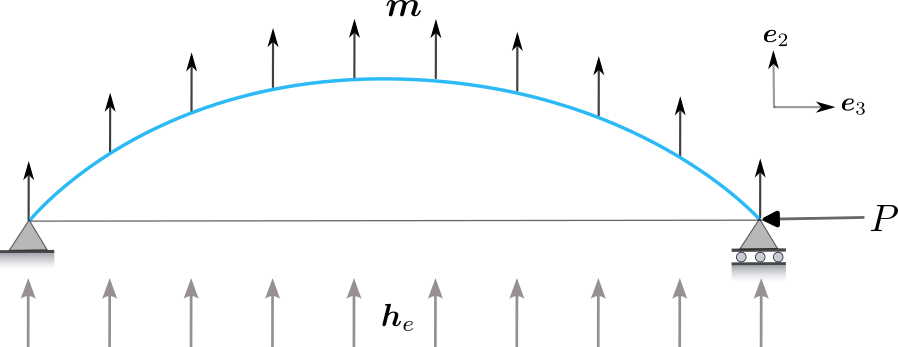
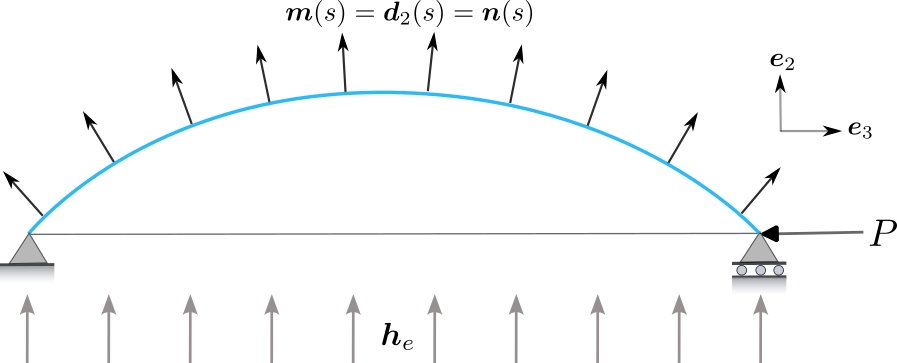
A hard ferromagnet is a ferromagnet with very large magnetic anisotropy energy (Ka>>1much-greater-thansubscript𝐾𝑎1K_{a}>>1). The magnetic anisotropy energy is minimised when the magnetization vector aligns along a preferred direction within the ferromagnetic solid. Thus, in a hard ferromagnetic ribbon, magnetization vector (𝒎(s¯)𝒎¯𝑠{\bf\it m}(\bar{s})) makes a constant angle with the tangent (𝒅3(s¯)subscript𝒅3¯𝑠{\bf\it d}_{3}(\bar{s})) along the entire length of the curve. 𝒎(s¯)𝒎¯𝑠{\bf\it m}(\bar{s}) varies spatially along the length of the curve to maintain a constant angle with the tangent of the curve as the ribbon deforms. We will consider that 𝒎(s¯)𝒎¯𝑠{\bf\it m}(\bar{s}) is either aligned along the normal (𝒎(s¯)𝒅3(s¯)perpendicular-to𝒎¯𝑠subscript𝒅3¯𝑠{\bf\it m}(\bar{s})\perp{\bf\it d}_{3}(\bar{s})) or that it is aligned along the tangent (𝒎(s¯)𝒅3(s¯)conditional𝒎¯𝑠subscript𝒅3¯𝑠{\bf\it m}(\bar{s})\parallel{\bf\it d}_{3}(\bar{s})) of the curve 𝒓(s¯)𝒓¯𝑠{{\bf\it r}}(\bar{s}), see Figs. 5(a) and 5(b). Note that, in this case (𝒎𝒏)2superscript𝒎𝒏2({\bf\it m}\cdot{\bf\it n})^{2} is constant and hence the demag. energy does not participate in energy minimization. The deformation in this case is driven by the interplay among Zeeman energy, bending energy, and loading device energy. We study the deformation of a hard ferromagnetic ribbon with the external magnetic field aligned in both the transverse and axial directions.

In this case, the magnetization direction reorients as a result of induced deformation due to the presence of 𝒉esubscript𝒉𝑒{\bf\it h}_{e}. The magnetization vector field for the deformed configuration is given by

𝒎(s¯)=(0,sinϕ(s¯),cosϕ(s¯)).𝒎¯𝑠0italic-ϕ¯𝑠italic-ϕ¯𝑠{\bf\it m}(\bar{s})=(0,\sin\phi(\bar{s}),\cos\phi(\bar{s})). (28)

Substituting this expression of 𝒎(s¯)𝒎¯𝑠{\bf\it m}(\bar{s}) in Eqn. 20 leads us to

¯(θ,ψ)=1201(θ(s¯))2𝑑s¯+K¯d01sin2(ϕ(s¯)θ(s¯))𝑑s¯2K¯dhe01cos(ϕ(s¯)ψ)𝑑s¯+P¯01cosθ(s¯)𝑑s¯Q¯01sinθ(s¯)𝑑s¯P¯¯𝜃𝜓12superscriptsubscript01superscriptsuperscript𝜃¯𝑠2differential-d¯𝑠subscript¯𝐾𝑑superscriptsubscript01superscript2italic-ϕ¯𝑠𝜃¯𝑠differential-d¯𝑠2subscript¯𝐾𝑑subscript𝑒superscriptsubscript01italic-ϕ¯𝑠𝜓differential-d¯𝑠¯𝑃superscriptsubscript01𝜃¯𝑠differential-d¯𝑠¯𝑄superscriptsubscript01𝜃¯𝑠differential-d¯𝑠¯𝑃\begin{split}\bar{\mathcal{E}}(\theta,\psi)=\frac{1}{2}\int_{0}^{1}(\theta^{\prime}(\bar{s}))^{2}d\bar{s}+\bar{K}_{d}\int_{0}^{1}\sin^{2}(\phi(\bar{s})-\theta(\bar{s}))d\bar{s}-2\bar{K}_{d}h_{e}\int_{0}^{1}\cos(\phi(\bar{s})-\psi)d\bar{s}\\ +\bar{P}\int_{0}^{1}\cos\theta(\bar{s})d\bar{s}-\bar{Q}\int_{0}^{1}\sin\theta(\bar{s})d\bar{s}-\bar{P}\end{split} (29)

where Q¯¯𝑄\bar{Q} is a Lagrange multiplier introduced to distinguish from R¯¯𝑅\bar{R}. Recall R¯¯𝑅\bar{R} is the vertical reaction for the Euler’s Elastica (see Eqn. 27). Following similar steps as in soft magnetization scenario, we arrive at the following Euler-Lagrange equations for hard magnetization case as

θ′′(s¯)+P¯sinθ(s¯)2K¯dhesin(ϕ(s¯)ψ)+Qcosθ(s¯)superscript𝜃′′¯𝑠¯𝑃𝜃¯𝑠2subscript¯𝐾𝑑subscript𝑒italic-ϕ¯𝑠𝜓𝑄𝜃¯𝑠\displaystyle\theta^{\prime\prime}(\bar{s})+\bar{P}\sin\theta(\bar{s})-2\bar{K}_{d}h_{e}\sin(\phi(\bar{s})-\psi)+Q\cos\theta(\bar{s}) =0,absent0\displaystyle=0, (30)
θ(s¯)η(s¯)|s¯=0\displaystyle\theta^{\prime}(\bar{s})\eta(\bar{s})\rvert_{\bar{s}=0} =0,absent0\displaystyle=0,
θ(s¯)η(s¯)|s¯=1\displaystyle\theta^{\prime}(\bar{s})\eta(\bar{s})\rvert_{\bar{s}=1} =0.absent0\displaystyle=0.

We consider tangential and normal uniform magnetization distributions such that ϕ(s¯)=θ(s¯),θ(s¯)+π2italic-ϕ¯𝑠𝜃¯𝑠𝜃¯𝑠𝜋2\phi(\bar{s})=\theta(\bar{s}),\theta(\bar{s})+\frac{\pi}{2} respectively. We expose the hard ferromagnetic ribbon to axial and transverse external magnetic fields, i.e., ψ=0,π2𝜓0𝜋2\psi=0,\frac{\pi}{2}. The corresponding equilibrium equations are enumerated as

𝒉e=𝒆3:𝒎(s¯)=𝒕(s¯):θ′′(s¯)+(P¯2K¯dhe)sinθ(s¯)+Q¯cosθ(s¯)=0,𝒎(s¯)=𝒏(s¯):θ′′(s¯)+P¯sinθ(s¯)+(Q¯2K¯dhe)cosθ(s¯)=0,𝒉e=𝒆2:𝒎(s¯)=𝒕(s¯):θ′′(s¯)+P¯sinθ(s¯)+(Q¯+2K¯dhe)cosθ(s¯)=0,𝒎(s¯)=𝒏(s¯):θ′′(s¯)+(P¯2K¯dhe)sinθ(s¯)+Q¯cosθ(s¯)=0.:subscript𝒉𝑒subscript𝒆3𝒎¯𝑠𝒕¯𝑠:formulae-sequencesuperscript𝜃′′¯𝑠¯𝑃2subscript¯𝐾𝑑subscript𝑒𝜃¯𝑠¯𝑄𝜃¯𝑠0𝒎¯𝑠𝒏¯𝑠:formulae-sequencesuperscript𝜃′′¯𝑠¯𝑃𝜃¯𝑠¯𝑄2subscript¯𝐾𝑑subscript𝑒𝜃¯𝑠0subscript𝒉𝑒subscript𝒆2:𝒎¯𝑠𝒕¯𝑠:formulae-sequencesuperscript𝜃′′¯𝑠¯𝑃𝜃¯𝑠¯𝑄2subscript¯𝐾𝑑subscript𝑒𝜃¯𝑠0𝒎¯𝑠𝒏¯𝑠:superscript𝜃′′¯𝑠¯𝑃2subscript¯𝐾𝑑subscript𝑒𝜃¯𝑠¯𝑄𝜃¯𝑠0\begin{split}{\bf\it h}_{e}={\bf\it e}_{3}:{\bf\it m}(\bar{s})={\bf\it t}(\bar{s}):&\quad\theta^{\prime\prime}(\bar{s})+(\bar{P}-2\bar{K}_{d}h_{e})\sin\theta(\bar{s})+\bar{Q}\cos\theta(\bar{s})=0,\\ {\bf\it m}(\bar{s})={\bf\it n}(\bar{s}):&\quad\theta^{\prime\prime}(\bar{s})+\bar{P}\sin\theta(\bar{s})+(\bar{Q}-2\bar{K}_{d}h_{e})\cos\theta(\bar{s})=0,\\ {\bf\it h}_{e}={\bf\it e}_{2}:{\bf\it m}(\bar{s})={\bf\it t}(\bar{s}):&\quad\theta^{\prime\prime}(\bar{s})+\bar{P}\sin\theta(\bar{s})+(\bar{Q}+2\bar{K}_{d}h_{e})\cos\theta(\bar{s})=0,\\ {\bf\it m}(\bar{s})={\bf\it n}(\bar{s}):&\quad\theta^{\prime\prime}(\bar{s})+(\bar{P}-2\bar{K}_{d}h_{e})\sin\theta(\bar{s})+\bar{Q}\cos\theta(\bar{s})=0.\end{split} (31)
Refer to caption
(a)
Refer to caption
(b)
Figure 5: Magnetically hard ferromagnetic ribbon under the influence of an external magnetic field: (a) Magnetization along the tangential direction, (b) Magnetization along the normal direction.

3 Path continuation methodology

We determine numerical solutions to the equilibrium equations as the loading parameter P¯¯𝑃\bar{P} is quasi-statically varied for various loading scenarios. We utilize a continuation method called pseudo arc length-based technique as discussed in Peletan2014 to determine the deformed configurations. The technique constrains the incremental deformation measure and increment in load parameters (P,R𝑃𝑅P,R) via a hyperspheric constraint.

3.1 Discretization of equilibrium equations

We discretize Eqn. (24) for fixed-fixed boundary conditions. We discretize the domain into N+1𝑁1N+1 nodal points as s¯i=ih;i=0,1,,N+1formulae-sequencesubscript¯𝑠𝑖𝑖𝑖01𝑁1\bar{s}_{i}=ih;i=0,1,\dots,N+1 where h=1N+11𝑁1h=\frac{1}{N+1}. We utilize second-order accurate central difference scheme to approximate the second-order derivative in Eqn. (24). The discrete system of equations alongwith the boundary conditions is

θi12θi+θi+1h2+P¯sinθi+K¯dsin2θi+R¯cosθisubscript𝜃𝑖12subscript𝜃𝑖subscript𝜃𝑖1superscript2¯𝑃subscript𝜃𝑖subscript¯𝐾𝑑2subscript𝜃𝑖¯𝑅subscript𝜃𝑖\displaystyle\frac{\theta_{i-1}-2\theta_{i}+\theta_{i+1}}{h^{2}}+\bar{P}\sin\theta_{i}+\bar{K}_{d}\sin 2\theta_{i}+\bar{R}\cos\theta_{i} =0;i=1,2,,N,formulae-sequenceabsent0𝑖12𝑁\displaystyle=0;\qquad i=1,2,\dots,N, (32)
θ0=0,θN+1=0,formulae-sequencesubscript𝜃00subscript𝜃𝑁10\displaystyle\theta_{0}=0,\theta_{N+1}=0,

where θisubscript𝜃𝑖\theta_{i} denotes the numerical counterpart of θ(s¯=s¯i)𝜃¯𝑠subscript¯𝑠𝑖\theta(\bar{s}=\bar{s}_{i}). In matrix-vector form, the discretized system can be written for all three cases (for fixed-free case where R¯=0¯𝑅0\bar{R}=0) as

𝑲𝜽+P¯sin𝜽+K¯dsin2𝜽+R¯cos𝜽=0 (see appendix B for 𝑲 and 𝜽).\displaystyle{\bf\it K\theta}+\bar{P}\sin{\bf\it\theta}+\bar{K}_{d}\sin 2{\bf\it\theta}+\bar{R}\cos{\bf\it\theta}={\bf\it 0}\text{ (see appendix \ref{app:equilibrium} for ${\bf\it K}$ and ${\bf\it\theta}$}). (33)

Incorporating the discretized form of integral constraint (Eqn. (26)) results in the combined nonlinear system of equations (for fixed-fixed and pinned-pinned conditions)

(𝑲𝜽+P¯sin𝜽+K¯dsin2𝜽+R¯cos𝜽sinθ1++sinθN)=(00), or, 𝒇(𝜽,R¯,P¯)=0.formulae-sequencematrix𝑲𝜽¯𝑃𝜽subscript¯𝐾𝑑2𝜽¯𝑅𝜽subscript𝜃1subscript𝜃𝑁matrixbold-italic-00 or, 𝒇𝜽¯𝑅¯𝑃bold-italic-0\begin{split}\begin{pmatrix}{\bf\it K\theta}+\bar{P}\sin{\bf\it\theta}+\bar{K}_{d}\sin 2{\bf\it\theta}+\bar{R}\cos{\bf\it\theta}\\ \sin\theta_{1}+\dots+\sin\theta_{N}\end{pmatrix}&=\begin{pmatrix}{\bf\it 0}\\ 0\end{pmatrix},\\ \text{ or, }\qquad\qquad{\bf\it f}({\bf\it\theta},\bar{R},\bar{P})={\bf\it 0}.&\end{split} (34)

3.2 Pseudo arc length-based continuation method

We proceed to devise a strategy to solve the nonlinear system of equations (Eqn. (34)) using an arc length-based continuation method. Let us describe k𝑘k-th configuration of the planar-deforming ferromagnetic ribbon as (𝜽k,R¯k,P¯k)subscript𝜽𝑘subscript¯𝑅𝑘subscript¯𝑃𝑘({\bf\it\theta}_{k},\bar{R}_{k},\bar{P}_{k}) where k𝑘k denotes the configuration index. The algorithm works in two steps: prediction step and correction step.

Prediction step

: We expand the equilibrium equation (Eqn. (34)) at (k+1)𝑘1(k+1)-th index in terms of Taylor series expansion about k𝑘k as

𝒇(𝜽k+1,R¯k+1,P¯k+1)=0=𝒇(𝜽k,R¯k,P¯k)=0+𝒇𝜽|kΔ𝜽k+𝒇R¯|kΔR¯k+𝒇P¯|kΔP¯k+𝒪(Δ𝜽k2,ΔR¯k2,ΔP¯k2)ignore,\displaystyle\underbrace{{\bf\it f}({\bf\it\theta}_{k+1},\bar{R}_{k+1},\bar{P}_{k+1})}_{={\bf\it 0}}=\underbrace{{\bf\it f}({\bf\it\theta}_{k},\bar{R}_{k},\bar{P}_{k})}_{={\bf\it 0}}+\partialderivative{{\bf\it f}}{{\bf\it\theta}}\bigg{\rvert}_{k}\Delta{\bf\it\theta}_{k}+\partialderivative{{\bf\it f}}{\bar{R}}\bigg{\rvert}_{k}\Delta\bar{R}_{k}+\partialderivative{{\bf\it f}}{\bar{P}}\bigg{\rvert}_{k}\Delta\bar{P}_{k}+\underbrace{\mathcal{O}(\Delta{\bf\it\theta}_{k}^{2},\Delta\bar{R}_{k}^{2},\Delta\bar{P}_{k}^{2})}_{\text{ignore}}, (35)
𝒇𝜽|kΔ𝜽k+𝒇R¯|kΔR¯k+𝒇P¯|kΔP¯k\displaystyle\implies\partialderivative{{\bf\it f}}{{\bf\it\theta}}\bigg{\rvert}_{k}\Delta{\bf\it\theta}_{k}+\partialderivative{{\bf\it f}}{\bar{R}}\bigg{\rvert}_{k}\Delta\bar{R}_{k}+\partialderivative{{\bf\it f}}{\bar{P}}\bigg{\rvert}_{k}\Delta\bar{P}_{k} =0.absentbold-italic-0\displaystyle={\bf\it 0}. (36)

We define a tangent vector as

𝒆ksubscript𝒆𝑘\displaystyle{\bf\it e}_{k} =(Δ𝜽kΔR¯kΔP¯k),absentmatrixΔsubscript𝜽𝑘Δsubscript¯𝑅𝑘Δsubscript¯𝑃𝑘\displaystyle=\begin{pmatrix}\Delta{\bf\it\theta}_{k}\\ \Delta\bar{R}_{k}\\ \Delta\bar{P}_{k}\end{pmatrix}, (37)

whose norm squared is

𝒆k2=(Δ𝜽k)T(Δ𝜽k)+(ΔR¯k)2+(ΔP¯k)2.superscriptnormsubscript𝒆𝑘2superscriptΔsubscript𝜽𝑘𝑇Δsubscript𝜽𝑘superscriptΔsubscript¯𝑅𝑘2superscriptΔsubscript¯𝑃𝑘2\displaystyle\norm{{\bf\it e}_{k}}^{2}=(\Delta{\bf\it\theta}_{k})^{T}(\Delta{\bf\it\theta}_{k})+(\Delta\bar{R}_{k})^{2}+(\Delta\bar{P}_{k})^{2}. (38)

We make the following substitution

ΔP¯k=ak,ΔR¯k=akΔrk,Δ𝜽k=akΔϕk.formulae-sequenceΔsubscript¯𝑃𝑘subscript𝑎𝑘formulae-sequenceΔsubscript¯𝑅𝑘subscript𝑎𝑘Δsubscript𝑟𝑘Δsubscript𝜽𝑘subscript𝑎𝑘Δsubscriptbold-italic-ϕ𝑘\Delta\bar{P}_{k}=a_{k},\leavevmode\nobreak\ \Delta\bar{R}_{k}=a_{k}\Delta r_{k},\leavevmode\nobreak\ \Delta{\bf\it\theta}_{k}=a_{k}\Delta{\bf\it\phi}_{k}. (39)

Setting the norm of 𝒆ksubscript𝒆𝑘{\bf\it e}_{k} to unity, we obtain the expression for aksubscript𝑎𝑘a_{k}

ak2(Δϕk)T(Δϕk)+ak2(Δrk)2+ak2superscriptsubscript𝑎𝑘2superscriptΔsubscriptbold-italic-ϕ𝑘𝑇Δsubscriptbold-italic-ϕ𝑘superscriptsubscript𝑎𝑘2superscriptΔsubscript𝑟𝑘2superscriptsubscript𝑎𝑘2\displaystyle a_{k}^{2}(\Delta{\bf\it\phi}_{k})^{T}(\Delta{\bf\it\phi}_{k})+a_{k}^{2}(\Delta r_{k})^{2}+a_{k}^{2} =1,absent1\displaystyle=1, (40)
akabsentsubscript𝑎𝑘\displaystyle\implies a_{k} =±1(Δϕk)T(Δϕk)+(Δrk)2+1.absentplus-or-minus1superscriptΔsubscriptbold-italic-ϕ𝑘𝑇Δsubscriptbold-italic-ϕ𝑘superscriptΔsubscript𝑟𝑘21\displaystyle=\pm\frac{1}{\sqrt{(\Delta{\bf\it\phi}_{k})^{T}(\Delta{\bf\it\phi}_{k})+(\Delta r_{k})^{2}+1}}. (41)

The sign of aksubscript𝑎𝑘a_{k} is chosen positive if 𝒆k1T𝒆k>0superscriptsubscript𝒆𝑘1𝑇subscript𝒆𝑘0{\bf\it e}_{k-1}^{T}{\bf\it e}_{k}>0 or else aksubscript𝑎𝑘a_{k} is taken to be negative. Substituting the expressions for Δ𝜽k,ΔR¯kΔsubscript𝜽𝑘Δsubscript¯𝑅𝑘\Delta{\bf\it\theta}_{k},\Delta\bar{R}_{k} and ΔP¯kΔsubscript¯𝑃𝑘\Delta\bar{P}_{k} in Eqn. (36), we have

𝒇𝜽|kakΔϕk+𝒇R¯|kakΔrk+𝒇P¯|kak\displaystyle\partialderivative{{\bf\it f}}{{\bf\it\theta}}\bigg{\rvert}_{k}a_{k}\Delta{\bf\it\phi}_{k}+\partialderivative{{\bf\it f}}{\bar{R}}\bigg{\rvert}_{k}a_{k}\Delta r_{k}+\partialderivative{{\bf\it f}}{\bar{P}}\bigg{\rvert}_{k}a_{k} =0,absentbold-italic-0\displaystyle={\bf\it 0}, (42)
[𝒇𝜽|k𝒇R¯|k](ΔϕkΔrk)=𝒇P¯|k.\displaystyle\implies\begin{bmatrix}\partialderivative{{\bf\it f}}{{\bf\it\theta}}\bigg{\rvert}_{k}&\partialderivative{{\bf\it f}}{\bar{R}}\bigg{\rvert}_{k}\end{bmatrix}\begin{pmatrix}\Delta{\bf\it\phi}_{k}\\ \Delta r_{k}\end{pmatrix}=-\partialderivative{{\bf\it f}}{\bar{P}}\bigg{\rvert}_{k}. (43)

We use Eqn. (43) to solve for Δϕk,ΔrkΔsubscriptbold-italic-ϕ𝑘Δsubscript𝑟𝑘\Delta{\bf\it\phi}_{k},\Delta r_{k} and then compute aksubscript𝑎𝑘a_{k} (Eqn. (41)) and 𝒆ksubscript𝒆𝑘{\bf\it e}_{k} (Eqn. (37)). We now construct the initial guess for (k+1)𝑘1(k+1)-configuration as

(𝜽k+1(0)R¯k+1(0)P¯k+1(0))matrixsuperscriptsubscript𝜽𝑘10superscriptsubscript¯𝑅𝑘10superscriptsubscript¯𝑃𝑘10\displaystyle\begin{pmatrix}{\bf\it\theta}_{k+1}^{(0)}\\ \bar{R}_{k+1}^{(0)}\\ \bar{P}_{k+1}^{(0)}\end{pmatrix} =(𝜽kR¯kP¯k)+Δs𝒆k,absentmatrixsubscript𝜽𝑘subscript¯𝑅𝑘subscript¯𝑃𝑘Δ𝑠subscript𝒆𝑘\displaystyle=\begin{pmatrix}{\bf\it\theta}_{k}\\ \bar{R}_{k}\\ \bar{P}_{k}\end{pmatrix}+\Delta s\cdot{\bf\it e}_{k}, (44)

where ΔsΔ𝑠\Delta s is the arc length step size. ΔsΔ𝑠\Delta s is small enough to capture the bifurcation along the equilibrium path.

Correction step

: We subject the predicted initial guess (Eqn. (44)) of (k+1)𝑘1(k+1)-configuration to a sequence of corrective iterations using the widely-used Newton-Raphson technique. Denoting (k+1)𝑘1(k+1)-configuration by (𝜽k+1,R¯k+1,P¯k+1)subscript𝜽𝑘1subscript¯𝑅𝑘1subscript¯𝑃𝑘1({\bf\it\theta}_{k+1},\bar{R}_{k+1},\bar{P}_{k+1}), we obtain the following Taylor series expansion about l𝑙l-iteration level

𝒇(𝜽k+1,R¯k+1,P¯k+1)=0𝒇(𝜽k+1(l),R¯k+1(l),P¯k+1(l))+𝒇𝜽|k+1(l)Δ𝜽k+1(l+1)+𝒇R¯|k+1(l)ΔR¯k+1(l+1)+𝒇P¯|k+1(l)ΔP¯k+1(l+1),\displaystyle\underbrace{{\bf\it f}({\bf\it\theta}_{k+1},\bar{R}_{k+1},\bar{P}_{k+1})}_{={\bf\it 0}}\approx{\bf\it f}({\bf\it\theta}_{k+1}^{(l)},\bar{R}_{k+1}^{(l)},\bar{P}_{k+1}^{(l)})+\partialderivative{{\bf\it f}}{{\bf\it\theta}}\bigg{\rvert}_{k+1}^{(l)}\Delta{\bf\it\theta}_{k+1}^{(l+1)}+\partialderivative{{\bf\it f}}{\bar{R}}\bigg{\rvert}_{k+1}^{(l)}\Delta\bar{R}_{k+1}^{(l+1)}+\partialderivative{{\bf\it f}}{\bar{P}}\bigg{\rvert}_{k+1}^{(l)}\Delta\bar{P}_{k+1}^{(l+1)}, (45)
𝒇𝜽|k+1(l)Δ𝜽k+1(l+1)+𝒇R¯|k+1(l)ΔR¯k+1(l+1)+𝒇P¯|k+1(l)ΔP¯k+1(l+1)=𝒇(𝜽k+1(l),R¯k+1(l),P¯k+1(l)).\displaystyle\implies\partialderivative{{\bf\it f}}{{\bf\it\theta}}\bigg{\rvert}_{k+1}^{(l)}\Delta{\bf\it\theta}_{k+1}^{(l+1)}+\partialderivative{{\bf\it f}}{\bar{R}}\bigg{\rvert}_{k+1}^{(l)}\Delta\bar{R}_{k+1}^{(l+1)}+\partialderivative{{\bf\it f}}{\bar{P}}\bigg{\rvert}_{k+1}^{(l)}\Delta\bar{P}_{k+1}^{(l+1)}=-{\bf\it f}({\bf\it\theta}_{k+1}^{(l)},\bar{R}_{k+1}^{(l)},\bar{P}_{k+1}^{(l)}). (46)

We enforce the orthogonality constraint on tangent vector at every iteration level l𝑙l, which is

𝒆kT𝒆k+1(l+1)superscriptsubscript𝒆𝑘𝑇superscriptsubscript𝒆𝑘1𝑙1\displaystyle{\bf\it e}_{k}^{T}{\bf\it e}_{k+1}^{(l+1)} =0,absent0\displaystyle=0, (47)
(Δ𝜽k)T(Δ𝜽k+1(l+1))+(ΔR¯k)(ΔR¯k+1(l+1))+(ΔP¯k)(ΔP¯k+1(l+1))absentsuperscriptΔsubscript𝜽𝑘𝑇Δsuperscriptsubscript𝜽𝑘1𝑙1Δsubscript¯𝑅𝑘Δsuperscriptsubscript¯𝑅𝑘1𝑙1Δsubscript¯𝑃𝑘Δsuperscriptsubscript¯𝑃𝑘1𝑙1\displaystyle\implies(\Delta{\bf\it\theta}_{k})^{T}(\Delta{\bf\it\theta}_{k+1}^{(l+1)})+(\Delta\bar{R}_{k})(\Delta\bar{R}_{k+1}^{(l+1)})+(\Delta\bar{P}_{k})(\Delta\bar{P}_{k+1}^{(l+1)}) =0.absent0\displaystyle=0. (48)

Combining Eqns. (46) and (48) to construct the following iterative scheme

[𝒇𝜽|k+1(l)𝒇R¯|k+1(l)𝒇P¯|k+1(l)(Δ𝜽k)TΔR¯kΔP¯k](Δ𝜽k+1(l+1)ΔR¯k+1(l+1)ΔP¯k+1(l+1))=(𝒇(𝜽k+1(l),R¯k+1(l),P¯k+1(l))0).\displaystyle\begin{bmatrix}\partialderivative{{\bf\it f}}{{\bf\it\theta}}\bigg{\rvert}_{k+1}^{(l)}&\partialderivative{{\bf\it f}}{\bar{R}}\bigg{\rvert}_{k+1}^{(l)}&\partialderivative{{\bf\it f}}{\bar{P}}\bigg{\rvert}_{k+1}^{(l)}\\ (\Delta{\bf\it\theta}_{k})^{T}&\Delta\bar{R}_{k}&\Delta\bar{P}_{k}\end{bmatrix}\begin{pmatrix}\Delta{\bf\it\theta}_{k+1}^{(l+1)}\\ \Delta\bar{R}_{k+1}^{(l+1)}\\ \Delta\bar{P}_{k+1}^{(l+1)}\end{pmatrix}=\begin{pmatrix}-{\bf\it f}({\bf\it\theta}_{k+1}^{(l)},\bar{R}_{k+1}^{(l)},\bar{P}_{k+1}^{(l)})\\ 0\end{pmatrix}. (49)

We solve the matrix equation (Eqn. (49)) and then carry out the update procedure as

(𝜽k+1(l+1)R¯k+1(l+1)P¯k+1(l+1))=(𝜽k+1(l)R¯k+1(l)P¯k+1(l))+(Δ𝜽k+1(l+1)ΔR¯k+1(l+1)ΔP¯k+1(l+1)).matrixsuperscriptsubscript𝜽𝑘1𝑙1superscriptsubscript¯𝑅𝑘1𝑙1superscriptsubscript¯𝑃𝑘1𝑙1matrixsuperscriptsubscript𝜽𝑘1𝑙superscriptsubscript¯𝑅𝑘1𝑙superscriptsubscript¯𝑃𝑘1𝑙matrixΔsuperscriptsubscript𝜽𝑘1𝑙1Δsuperscriptsubscript¯𝑅𝑘1𝑙1Δsuperscriptsubscript¯𝑃𝑘1𝑙1\displaystyle\begin{pmatrix}{\bf\it\theta}_{k+1}^{(l+1)}\\ \bar{R}_{k+1}^{(l+1)}\\ \bar{P}_{k+1}^{(l+1)}\end{pmatrix}=\begin{pmatrix}{\bf\it\theta}_{k+1}^{(l)}\\ \bar{R}_{k+1}^{(l)}\\ \bar{P}_{k+1}^{(l)}\end{pmatrix}+\begin{pmatrix}\Delta{\bf\it\theta}_{k+1}^{(l+1)}\\ \Delta\bar{R}_{k+1}^{(l+1)}\\ \Delta\bar{P}_{k+1}^{(l+1)}\end{pmatrix}. (50)

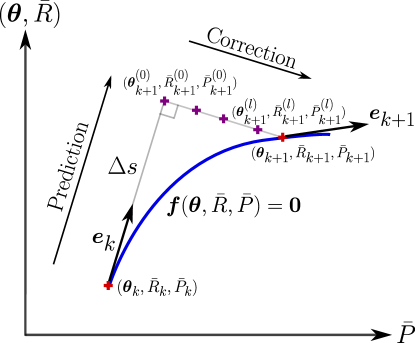
The correction steps (l=1,2,𝑙12l=1,2,\dots) are performed till the increments meet a prescribed tolerance. We then increment the configuration index (kk+1𝑘𝑘1k\leftarrow k+1) and repeat the prediction and correction steps until P¯maxsubscript¯𝑃max\bar{P}_{\text{max}} is reached. The adopted continuation procedure is illustrated in Fig. 6.
Refer to caption
Figure 6: Schematic of pseudo arc length-based continuation procedure showing equilibrium curve in blue.

4 Bifurcation analysis of equilibrium configuration

We now determine whether a given deformed equilibrium configuration is stable with respect to infinitesimal perturbations. Stable perturbations are physically realizable. This requires evaluation of the second variational derivative of the energy functional at the critical points. The critical points are the solutions to the Euler-Lagrange equations.

We now determine the second variational derivative of the functional, δ2¯(θ)superscript𝛿2¯𝜃\delta^{2}\mathcal{\overline{E}}(\theta) for the soft magnetization ribbon when 𝒉esubscript𝒉𝑒{\bf\it h}_{e} is applied along 𝒆2subscript𝒆2{\bf\it e}_{2}-axis such that 𝒎(s¯)=𝒆2𝒎¯𝑠subscript𝒆2{\bf\it m}(\bar{s})={\bf\it e}_{2}. Introducing first order perturbation in the assumed extremum θ𝜃\theta as θ^(s¯)=θ(s¯)+ϵη(s¯)^𝜃¯𝑠𝜃¯𝑠italic-ϵ𝜂¯𝑠\hat{\theta}(\bar{s})=\theta(\bar{s})+\epsilon\eta(\bar{s}) where η(s¯)𝜂¯𝑠\eta(\bar{s}) is a kinematically admissible planar variation and ϵitalic-ϵ\epsilon is a small parameter, and substituting it into Eqn. (20)

¯(θ+ϵη)=1201(θ+ϵη)2𝑑s¯+K¯d01cos2(θ+ϵη)at𝑑s¯+P¯01cos(θ+ϵη)𝑑s¯R¯01sin(θ+ϵη)𝑑s¯+constant.¯𝜃italic-ϵ𝜂12superscriptsubscript01superscriptsuperscript𝜃italic-ϵsuperscript𝜂2differential-d¯𝑠subscript¯𝐾𝑑superscriptsubscript01superscript2𝜃italic-ϵ𝜂𝑎𝑡differential-d¯𝑠¯𝑃superscriptsubscript01𝜃italic-ϵ𝜂differential-d¯𝑠¯𝑅superscriptsubscript01𝜃italic-ϵ𝜂differential-d¯𝑠constant\mathcal{\overline{E}}(\theta+\epsilon\eta)=\frac{1}{2}\int_{0}^{1}(\theta^{\prime}+\epsilon\eta^{\prime})^{2}d\bar{s}+\bar{K}_{d}\int_{0}^{1}\cos^{2}(\theta+\epsilon\eta)atd\bar{s}+\bar{P}\int_{0}^{1}\cos(\theta+\epsilon\eta)d\bar{s}\\ -\bar{R}\int_{0}^{1}\sin(\theta+\epsilon\eta)d\bar{s}+\text{constant}. (51)

Simplifying the above expansion and taking into account the boundary conditions, we have

δ2¯(θ)=d2¯(θ+ϵη)dϵ2|ϵ=0\displaystyle\delta^{2}\mathcal{\overline{E}}(\theta)=\derivative[2]{\mathcal{\overline{E}}(\theta+\epsilon\eta)}{\epsilon}\bigg{\rvert}_{\epsilon=0} =01[η′′+2K¯dcos2θη+P¯cosθηR¯sinθη]η𝑑s¯,absentsuperscriptsubscript01delimited-[]superscript𝜂′′2subscript¯𝐾𝑑2𝜃𝜂¯𝑃𝜃𝜂¯𝑅𝜃𝜂𝜂differential-d¯𝑠\displaystyle=-\int_{0}^{1}[\eta^{\prime\prime}+2\bar{K}_{d}\cos 2\theta\eta+\bar{P}\cos\theta\eta-\bar{R}\sin\theta\eta]\eta d\bar{s}, (52)

for all kinematically admissible functions η(s¯)𝜂¯𝑠\eta(\bar{s}). The stability criterion states that

δ2¯(θ){>0 stable,<0 unstable.superscript𝛿2¯𝜃casesabsent0 stableabsent0 unstable\displaystyle\delta^{2}\mathcal{\overline{E}}(\theta)\begin{cases}>0&\text{ stable},\\ <0&\text{ unstable}.\end{cases} (53)

Further, we also introduce the first variation of the integral constraint 01sinθ(s¯)𝑑s¯=0superscriptsubscript01𝜃¯𝑠differential-d¯𝑠0\int_{0}^{1}\sin\theta(\bar{s})d\bar{s}=0 given as:

01cosθ(s¯)η(s¯)𝑑s¯=0.superscriptsubscript01𝜃¯𝑠𝜂¯𝑠differential-d¯𝑠0\displaystyle\int_{0}^{1}\cos\theta(\bar{s})\eta(\bar{s})d\bar{s}=0. (54)

The detailed bifurcation analysis technique is presented in Appendix C.

4.1 Construction of Sturm-Liouville problem

Following Levyakov2009 ; Bigoni2015 , we construct an equivalent Sturm-Liouville problem for the second variation δ2¯(θ)superscript𝛿2¯𝜃\delta^{2}\mathcal{\overline{E}}(\theta) as follows:

ϕn′′(s¯)+λn(2K¯dcos2θ+P¯cosθR¯sinθ)ϕn(s¯)=CRncosθ(s¯),superscriptsubscriptitalic-ϕ𝑛′′¯𝑠subscript𝜆𝑛2subscript¯𝐾𝑑2𝜃¯𝑃𝜃¯𝑅𝜃subscriptitalic-ϕ𝑛¯𝑠subscript𝐶subscript𝑅𝑛𝜃¯𝑠\displaystyle\phi_{n}^{\prime\prime}(\bar{s})+\lambda_{n}(2\bar{K}_{d}\cos 2\theta+\bar{P}\cos\theta-\bar{R}\sin\theta)\phi_{n}(\bar{s})=C_{R_{n}}\cos\theta(\bar{s}), (55)

where λnsubscript𝜆𝑛\lambda_{n} are the eigenvalues, ϕnsubscriptitalic-ϕ𝑛\phi_{n} the corresponding eigenmodes of Eqn. (55) and L(s¯)=(2K¯dcos2θ+P¯cosθR¯sinθ)𝐿¯𝑠2subscript¯𝐾𝑑2𝜃¯𝑃𝜃¯𝑅𝜃L(\bar{s})=(2\bar{K}_{d}\cos 2\theta+\bar{P}\cos\theta-\bar{R}\sin\theta) denotes the weight function. CRnsubscript𝐶subscript𝑅𝑛C_{R_{n}} is a Lagrange parameter introduced to enforce the isoperimetric constraint (Eqn. (54)). The conditions on ϕn(s¯)subscriptitalic-ϕ𝑛¯𝑠\phi_{n}(\bar{s}) are

  • fixed-fixed case: ϕn(0)=ϕn(1)=0subscriptitalic-ϕ𝑛0subscriptitalic-ϕ𝑛10\phi_{n}(0)=\phi_{n}(1)=0 and 01cosθ(s¯)ϕn(s¯)𝑑s¯=0superscriptsubscript01𝜃¯𝑠subscriptitalic-ϕ𝑛¯𝑠differential-d¯𝑠0\int_{0}^{1}\cos\theta(\bar{s})\phi_{n}(\bar{s})d\bar{s}=0,

  • pinned-pinned case: ϕn(0)=ϕn(1)=0superscriptsubscriptitalic-ϕ𝑛0superscriptsubscriptitalic-ϕ𝑛10\phi_{n}^{\prime}(0)=\phi_{n}^{\prime}(1)=0 and 01cosθ(s¯)ϕn(s¯)𝑑s¯=0superscriptsubscript01𝜃¯𝑠subscriptitalic-ϕ𝑛¯𝑠differential-d¯𝑠0\int_{0}^{1}\cos\theta(\bar{s})\phi_{n}(\bar{s})d\bar{s}=0,

  • fixed-free case: ϕn(0)=ϕn(1)=0subscriptitalic-ϕ𝑛0superscriptsubscriptitalic-ϕ𝑛10\phi_{n}(0)=\phi_{n}^{\prime}(1)=0.

We obtain the following conditions for two arbitrary eigenmodes ϕm(s¯)subscriptitalic-ϕ𝑚¯𝑠\phi_{m}(\bar{s}) and ϕn(s¯)subscriptitalic-ϕ𝑛¯𝑠\phi_{n}(\bar{s}) of the Sturm-Liouville problem (Eqn. (55))

λn01L(s¯)ϕn2𝑑s¯subscript𝜆𝑛superscriptsubscript01𝐿¯𝑠superscriptsubscriptitalic-ϕ𝑛2differential-d¯𝑠\displaystyle\lambda_{n}\int_{0}^{1}L(\bar{s})\phi_{n}^{2}d\bar{s} =01ϕn2𝑑s¯,absentsuperscriptsubscript01superscriptsubscriptitalic-ϕ𝑛2differential-d¯𝑠\displaystyle=\int_{0}^{1}\phi_{n}^{\prime 2}d\bar{s}, (56)

and the orthogonality condition

01L(s¯)ϕnϕm𝑑s¯superscriptsubscript01𝐿¯𝑠subscriptitalic-ϕ𝑛subscriptitalic-ϕ𝑚differential-d¯𝑠\displaystyle\int_{0}^{1}L(\bar{s})\phi_{n}\phi_{m}d\bar{s} =0.absent0\displaystyle=0. (57)

The details of the above calculation can be found in appendix C.

Spectral decomposition

: Let us use ϕn(s¯)subscriptitalic-ϕ𝑛¯𝑠\phi_{n}(\bar{s}) alongwith the weight function L(s¯)𝐿¯𝑠L(\bar{s}) to construct a Fourier series representation (converging in the mean) to the square-integrable function η(s¯)𝜂¯𝑠\eta(\bar{s}),

η(s¯)𝜂¯𝑠\displaystyle\eta(\bar{s}) =n=1cnϕn(s¯),cn are Fourier coefficients.absentsuperscriptsubscript𝑛1subscript𝑐𝑛subscriptitalic-ϕ𝑛¯𝑠subscript𝑐𝑛 are Fourier coefficients\displaystyle=\sum_{n=1}^{\infty}c_{n}\phi_{n}(\bar{s}),\qquad c_{n}\text{ are Fourier coefficients}. (58)

Substituting the above representation in Eqn. (52) and invoking the conditions (Eqns. (56) and (57)), we obtain the stability criterion:

δ2¯(θ)=n=1cn2(11λn)01(ϕn(s¯))2𝑑s¯{>0 if λn[0,1] stable,<0 if λn[0,1] unstable.superscript𝛿2¯𝜃superscriptsubscript𝑛1superscriptsubscript𝑐𝑛211subscript𝜆𝑛superscriptsubscript01superscriptsuperscriptsubscriptitalic-ϕ𝑛¯𝑠2differential-d¯𝑠casesabsent0 if subscript𝜆𝑛01 stableabsent0 if subscript𝜆𝑛01 unstable\displaystyle\delta^{2}\mathcal{\overline{E}}(\theta)=\sum_{n=1}^{\infty}c_{n}^{2}\bigg{(}1-\frac{1}{\lambda_{n}}\bigg{)}\int_{0}^{1}(\phi_{n}^{\prime}(\bar{s}))^{2}d\bar{s}\quad\begin{cases}>0\text{ if }\lambda_{n}\notin[0,1]&\text{ stable},\\ <0\text{ if }\lambda_{n}\in[0,1]&\text{ unstable}.\end{cases} (59)

4.1.1 Numerical bifurcation analysis

We describe the numerical procedure for the fixed-fixed case, which can be easily adapted to pinned-pinned and fixed-free cases. Given, Eqn. (55) as

ϕm′′(s¯)+λmLm(s¯)ϕm(s¯)superscriptsubscriptitalic-ϕ𝑚′′¯𝑠subscript𝜆𝑚subscript𝐿𝑚¯𝑠subscriptitalic-ϕ𝑚¯𝑠\displaystyle\phi_{m}^{\prime\prime}(\bar{s})+\lambda_{m}L_{m}(\bar{s})\phi_{m}(\bar{s}) =CRmN(s¯),absentsubscript𝐶subscript𝑅𝑚𝑁¯𝑠\displaystyle=C_{R_{m}}N(\bar{s}), (60)

where, the coefficient functions are

Lm(s¯)=2K¯dcos2θ(s¯)+P¯cosθ(s¯)R¯sinθ(s¯),N(s¯)=cosθ(s¯).formulae-sequencesubscript𝐿𝑚¯𝑠2subscript¯𝐾𝑑2𝜃¯𝑠¯𝑃𝜃¯𝑠¯𝑅𝜃¯𝑠𝑁¯𝑠𝜃¯𝑠L_{m}(\bar{s})=2\bar{K}_{d}\cos 2\theta(\bar{s})+\bar{P}\cos\theta(\bar{s})-\bar{R}\sin\theta(\bar{s}),\qquad N(\bar{s})=\cos\theta(\bar{s}). (61)

Eqn. (60) is also subjected to the boundary conditions ϕm(0)=0,ϕm(1)=0formulae-sequencesubscriptitalic-ϕ𝑚00subscriptitalic-ϕ𝑚10\phi_{m}(0)=0,\phi_{m}(1)=0 and the additional constraint

01ϕm(s¯)N(s¯)𝑑s¯superscriptsubscript01subscriptitalic-ϕ𝑚¯𝑠𝑁¯𝑠differential-d¯𝑠\displaystyle\int_{0}^{1}\phi_{m}(\bar{s})N(\bar{s})d\bar{s} =0.absent0\displaystyle=0. (62)
Numerical procedure to compute eigenvalues λmsubscript𝜆𝑚\lambda_{m}

: Partition the interval s¯[0,1]¯𝑠01\bar{s}\in[0,1] segments of equal length h=1n+11𝑛1h=\frac{1}{n+1} such that the starting points of the segments can be denoted by s¯i1=(i1)h;i=1,2,,n+1formulae-sequencesubscript¯𝑠𝑖1𝑖1𝑖12𝑛1\bar{s}_{i-1}=(i-1)h;i=1,2,\dots,n+1. For i𝑖i-th segment, the functions L(s¯)𝐿¯𝑠L(\bar{s}) and N(s¯)𝑁¯𝑠N(\bar{s}) are approximated by averaging their corresponding values at nodal indices i𝑖i and i+1𝑖1i+1 resulting in Lisubscript𝐿𝑖L_{i} and Nisubscript𝑁𝑖N_{i} respectively. Substituting these averaged quantities, Eqn. (60) becomes

ϕm′′(s¯)+λmLiϕm(s¯)=CRmNi,superscriptsubscriptitalic-ϕ𝑚′′¯𝑠subscript𝜆𝑚subscript𝐿𝑖subscriptitalic-ϕ𝑚¯𝑠subscript𝐶subscript𝑅𝑚subscript𝑁𝑖\displaystyle\phi_{m}^{\prime\prime}(\bar{s})+\lambda_{m}L_{i}\phi_{m}(\bar{s})=C_{R_{m}}N_{i}, (63)

which is an ordinary differential equation (ODE) with constant coefficients. The solution to this ODE is

ϕm(s¯)subscriptitalic-ϕ𝑚¯𝑠\displaystyle\phi_{m}(\bar{s}) =A1iF1i(s¯s¯i1)+A2iF2i(s¯s¯i1)+CRmNiλmLi,absentsubscript𝐴1𝑖subscript𝐹1𝑖¯𝑠subscript¯𝑠𝑖1subscript𝐴2𝑖subscript𝐹2𝑖¯𝑠subscript¯𝑠𝑖1subscript𝐶subscript𝑅𝑚subscript𝑁𝑖subscript𝜆𝑚subscript𝐿𝑖\displaystyle=A_{1i}F_{1i}(\bar{s}-\bar{s}_{i-1})+A_{2i}F_{2i}(\bar{s}-\bar{s}_{i-1})+C_{R_{m}}\frac{N_{i}}{\lambda_{m}L_{i}}, (64)

where A1isubscript𝐴1𝑖A_{1i} and A2isubscript𝐴2𝑖A_{2i} are constants, and the functions F1isubscript𝐹1𝑖F_{1i} and F2isubscript𝐹2𝑖F_{2i} are defined as

  1. 1.

    for λmLi>0subscript𝜆𝑚subscript𝐿𝑖0\lambda_{m}L_{i}>0 as F1i(s¯s¯i1)=cosai(s¯s¯i1),F2i(s¯s¯i1)=sinai(s¯s¯i1)formulae-sequencesubscript𝐹1𝑖¯𝑠subscript¯𝑠𝑖1subscript𝑎𝑖¯𝑠subscript¯𝑠𝑖1subscript𝐹2𝑖¯𝑠subscript¯𝑠𝑖1subscript𝑎𝑖¯𝑠subscript¯𝑠𝑖1F_{1i}(\bar{s}-\bar{s}_{i-1})=\cos a_{i}(\bar{s}-\bar{s}_{i-1}),\quad F_{2i}(\bar{s}-\bar{s}_{i-1})=\sin a_{i}(\bar{s}-\bar{s}_{i-1}),

  2. 2.

    for λmLi<0subscript𝜆𝑚subscript𝐿𝑖0\lambda_{m}L_{i}<0 as F1i(s¯s¯i1)=coshai(s¯s¯i1),F2i(s¯s¯i1)=sinai(s¯s¯i1)formulae-sequencesubscript𝐹1𝑖¯𝑠subscript¯𝑠𝑖1subscript𝑎𝑖¯𝑠subscript¯𝑠𝑖1subscript𝐹2𝑖¯𝑠subscript¯𝑠𝑖1subscript𝑎𝑖¯𝑠subscript¯𝑠𝑖1F_{1i}(\bar{s}-\bar{s}_{i-1})=\cosh a_{i}(\bar{s}-\bar{s}_{i-1}),\quad F_{2i}(\bar{s}-\bar{s}_{i-1})=\sin a_{i}(\bar{s}-\bar{s}_{i-1}) with ai=|λLi|subscript𝑎𝑖𝜆subscript𝐿𝑖a_{i}=\sqrt{\absolutevalue{\lambda L_{i}}}.

The constants A1isubscript𝐴1𝑖A_{1i} and A2isubscript𝐴2𝑖A_{2i} can be obtained from the matching conditions

ϕm(s¯i1)=ϕm,i1,ϕm(s¯i1)=ϕm,i1formulae-sequencesubscriptitalic-ϕ𝑚subscript¯𝑠𝑖1subscriptitalic-ϕ𝑚𝑖1superscriptsubscriptitalic-ϕ𝑚subscript¯𝑠𝑖1superscriptsubscriptitalic-ϕ𝑚𝑖1\phi_{m}(\bar{s}_{i-1})=\phi_{m,i-1},\qquad\phi_{m}^{\prime}(\bar{s}_{i-1})=\phi_{m,i-1}^{\prime} (65)

as

A1i=ϕm,i1CRmNiλmLi,A2i=ϕm,i1ai.formulae-sequencesubscript𝐴1𝑖subscriptitalic-ϕ𝑚𝑖1subscript𝐶subscript𝑅𝑚subscript𝑁𝑖subscript𝜆𝑚subscript𝐿𝑖subscript𝐴2𝑖superscriptsubscriptitalic-ϕ𝑚𝑖1subscript𝑎𝑖A_{1i}=\phi_{m,i-1}-C_{R_{m}}\frac{N_{i}}{\lambda_{m}L_{i}},\qquad A_{2i}=\frac{\phi_{m,i-1}^{\prime}}{a_{i}}. (66)

The quantity ϕm(s¯i)=ϕm,isubscriptitalic-ϕ𝑚subscript¯𝑠𝑖subscriptitalic-ϕ𝑚𝑖\phi_{m}(\bar{s}_{i})=\phi_{m,i} at the right end of the segment is computed alongwith its derivative as

ϕm,i=ϕm,i1F1i(h)+ϕm,i1aiF2i(h)+CRmNi[1F1i(h)]λmLi,ϕm,i=ϕm,i1F1i(h)+ϕm,i1aiF2i(h)CRmNiF1i(h)λmLi.formulae-sequencesubscriptitalic-ϕ𝑚𝑖subscriptitalic-ϕ𝑚𝑖1subscript𝐹1𝑖superscriptsubscriptitalic-ϕ𝑚𝑖1subscript𝑎𝑖subscript𝐹2𝑖subscript𝐶subscript𝑅𝑚subscript𝑁𝑖delimited-[]1subscript𝐹1𝑖subscript𝜆𝑚subscript𝐿𝑖subscriptsuperscriptitalic-ϕ𝑚𝑖subscriptitalic-ϕ𝑚𝑖1superscriptsubscript𝐹1𝑖superscriptsubscriptitalic-ϕ𝑚𝑖1subscript𝑎𝑖superscriptsubscript𝐹2𝑖subscript𝐶subscript𝑅𝑚subscript𝑁𝑖superscriptsubscript𝐹1𝑖subscript𝜆𝑚subscript𝐿𝑖\begin{split}\phi_{m,i}&=\phi_{m,i-1}F_{1i}(h)+\frac{\phi_{m,i-1}^{\prime}}{a_{i}}F_{2i}(h)+C_{R_{m}}N_{i}\frac{[1-F_{1i}(h)]}{\lambda_{m}L_{i}},\\ \phi^{\prime}_{m,i}&=\phi_{m,i-1}F_{1i}^{\prime}(h)+\frac{\phi_{m,i-1}^{\prime}}{a_{i}}F_{2i}^{\prime}(h)-C_{R_{m}}N_{i}\frac{F_{1i}^{\prime}(h)}{\lambda_{m}L_{i}}.\end{split} (67)

The general solution of Eqn. (63) can be constructed by using Eqns. (67), and the continuity requirement of ϕmsubscriptitalic-ϕ𝑚\phi_{m} and ϕmsuperscriptsubscriptitalic-ϕ𝑚\phi_{m}^{\prime} at the extremities of every integration segment. Since Eqn. (60) is linear, its general solution can be written as a combination of three particular solutions

ϕm(s¯)subscriptitalic-ϕ𝑚¯𝑠\displaystyle\phi_{m}(\bar{s}) =c1ψ1(s¯)+c2ψ2(s¯)+CRmψ3(s¯),absentsubscript𝑐1subscript𝜓1¯𝑠subscript𝑐2subscript𝜓2¯𝑠subscript𝐶subscript𝑅𝑚subscript𝜓3¯𝑠\displaystyle=c_{1}\psi_{1}(\bar{s})+c_{2}\psi_{2}(\bar{s})+C_{R_{m}}\psi_{3}(\bar{s}), (68)

where c1subscript𝑐1c_{1} and c2subscript𝑐2c_{2} are constants. We use the following initial data

ψ1(0)=1,ψ1(0)=0,CRm=0,ψ2(0)=0,ψ2(0)=1,CRm=0,ψ3(0)=0,ψ3(0)=0,CRm=1.\begin{split}&\psi_{1}(0)=1,\quad\psi_{1}^{\prime}(0)=0,\quad C_{R_{m}}=0,\\ &\psi_{2}(0)=0,\quad\psi_{2}^{\prime}(0)=1,\quad C_{R_{m}}=0,\\ &\psi_{3}(0)=0,\quad\psi_{3}^{\prime}(0)=0,\quad C_{R_{m}}=1.\end{split} (69)

The functions ψi(s¯),i=1,2,3formulae-sequencesubscript𝜓𝑖¯𝑠𝑖123\psi_{i}(\bar{s}),i=1,2,3 can be constructed separately using the recurrence relations Eqn. (67). Using boundary conditions, we have

ϕm(0)=0c1=0,ϕm(1)=0c2ψ2(1)+CRmψ3(1)=0.formulae-sequencesubscriptitalic-ϕ𝑚00subscript𝑐10subscriptitalic-ϕ𝑚10subscript𝑐2subscript𝜓21subscript𝐶subscript𝑅𝑚subscript𝜓310\begin{split}\phi_{m}(0)=0&\implies c_{1}=0,\\ \phi_{m}(1)=0&\implies c_{2}\psi_{2}(1)+C_{R_{m}}\psi_{3}(1)=0.\end{split} (70)

Substituting Eqn. (68) in Eqn. (62), the constraint can be rewritten as

c201ψ2(s¯)N(s¯)𝑑s¯+CRm01ψ3(s¯)N(s¯)𝑑s¯subscript𝑐2superscriptsubscript01subscript𝜓2¯𝑠𝑁¯𝑠differential-d¯𝑠subscript𝐶subscript𝑅𝑚superscriptsubscript01subscript𝜓3¯𝑠𝑁¯𝑠differential-d¯𝑠\displaystyle c_{2}\int_{0}^{1}\psi_{2}(\bar{s})N(\bar{s})d\bar{s}+C_{R_{m}}\int_{0}^{1}\psi_{3}(\bar{s})N(\bar{s})d\bar{s} =0.absent0\displaystyle=0. (71)

We construct the following homogeneous system of equations

[ψ2(1)ψ3(1)01ψ2(s¯)N(s¯)𝑑s¯01ψ3(s¯)N(s¯)𝑑s¯](c2CRm)=(00).matrixsubscript𝜓21subscript𝜓31superscriptsubscript01subscript𝜓2¯𝑠𝑁¯𝑠differential-d¯𝑠superscriptsubscript01subscript𝜓3¯𝑠𝑁¯𝑠differential-d¯𝑠matrixsubscript𝑐2subscript𝐶subscript𝑅𝑚matrix00\displaystyle\begin{bmatrix}\psi_{2}(1)&\psi_{3}(1)\\ \int_{0}^{1}\psi_{2}(\bar{s})N(\bar{s})d\bar{s}&\int_{0}^{1}\psi_{3}(\bar{s})N(\bar{s})d\bar{s}\end{bmatrix}\begin{pmatrix}c_{2}\\ C_{R_{m}}\end{pmatrix}=\begin{pmatrix}0\\ 0\end{pmatrix}. (72)

For non-trivial solution to the above equation, the determinant,

Δ=Δabsent\displaystyle\Delta= ψ2(1)01ψ3(s¯)N(s¯)𝑑s¯ψ3(1)01ψ2(s¯)N(s¯)𝑑s¯subscript𝜓21superscriptsubscript01subscript𝜓3¯𝑠𝑁¯𝑠differential-d¯𝑠subscript𝜓31superscriptsubscript01subscript𝜓2¯𝑠𝑁¯𝑠differential-d¯𝑠\displaystyle\psi_{2}(1)\int_{0}^{1}\psi_{3}(\bar{s})N(\bar{s})d\bar{s}-\psi_{3}(1)\int_{0}^{1}\psi_{2}(\bar{s})N(\bar{s})d\bar{s} (73)

must be zero. The integrals are evaluated numerically.
We vary the value of λmsubscript𝜆𝑚\lambda_{m} from 0 to 1 and monitor how ΔΔ\Delta changes

  • If at least one value of λm[0,1]subscript𝜆𝑚01\lambda_{m}\in[0,1] exists resulting in Δ=0Δ0\Delta=0, then the non-trivial solution of Eqn. (68) exists which also satisfies the boundary conditions. The corresponding equilibrium configuration is unstable.

  • It no λm[0,1]subscript𝜆𝑚01\lambda_{m}\in[0,1] results in Δ=0Δ0\Delta=0, it implies that there exists a trivial solution of Eqn. (68). The corresponding equilibrium configuration is therefore stable.

5 Results and Discussion

In this section, we begin with the validation of our numerical framework by comparing our results with the well-studied Euler’s Elastica from existing literature Bigoni2015 . We consider three canonical boundary conditions, namely, fixed-fixed, pinned-pinned, and fixed-free. Our results are presented as load-displacement curves, also known as equilibrium curves, which have been determined using the continuation algorithm described in Section 3. We use the well-known mathematical analysis tool, Auto-07p, to validate numerical results. We then explore solutions for both soft and hard ferromagnetic ribbons under different loading scenarios. We have summarised all the cases considered in Table 1. The width of the ferromagnetic ribbon is assumed to be very small, allowing it to deform into self-intersecting loops while remaining planar.

Sections 5.1 5.2 5.3
Description Euler’s Elastica Case 1 Soft ferromagnet Case 2: Hard ferromagnet
Transverse 𝒉esubscript𝒉𝑒{\bf\it h}_{e} Transverse 𝒉esubscript𝒉𝑒{\bf\it h}_{e} Axial 𝒉esubscript𝒉𝑒{\bf\it h}_{e}
𝒎=𝒕𝒎𝒕{\bf\it m}={\bf\it t} 𝒎=𝒏𝒎𝒏{\bf\it m}={\bf\it n} 𝒎=𝒕𝒎𝒕{\bf\it m}={\bf\it t} 𝒎=𝒏𝒎𝒏{\bf\it m}={\bf\it n}
Figures Fixed-Free (7) (10) (13) (7) but different R¯¯𝑅\bar{R} (7) but different R¯¯𝑅\bar{R} (13)
Fixed-Fixed (8) (11) (14) (8)        ,, (8)        ,, (14)
Pinned-Pinned (9) (12) (15) (9)        ,, (9)        ,, (15)
Table 1: Various considered cases in the study.

5.1 Euler’s Elastica

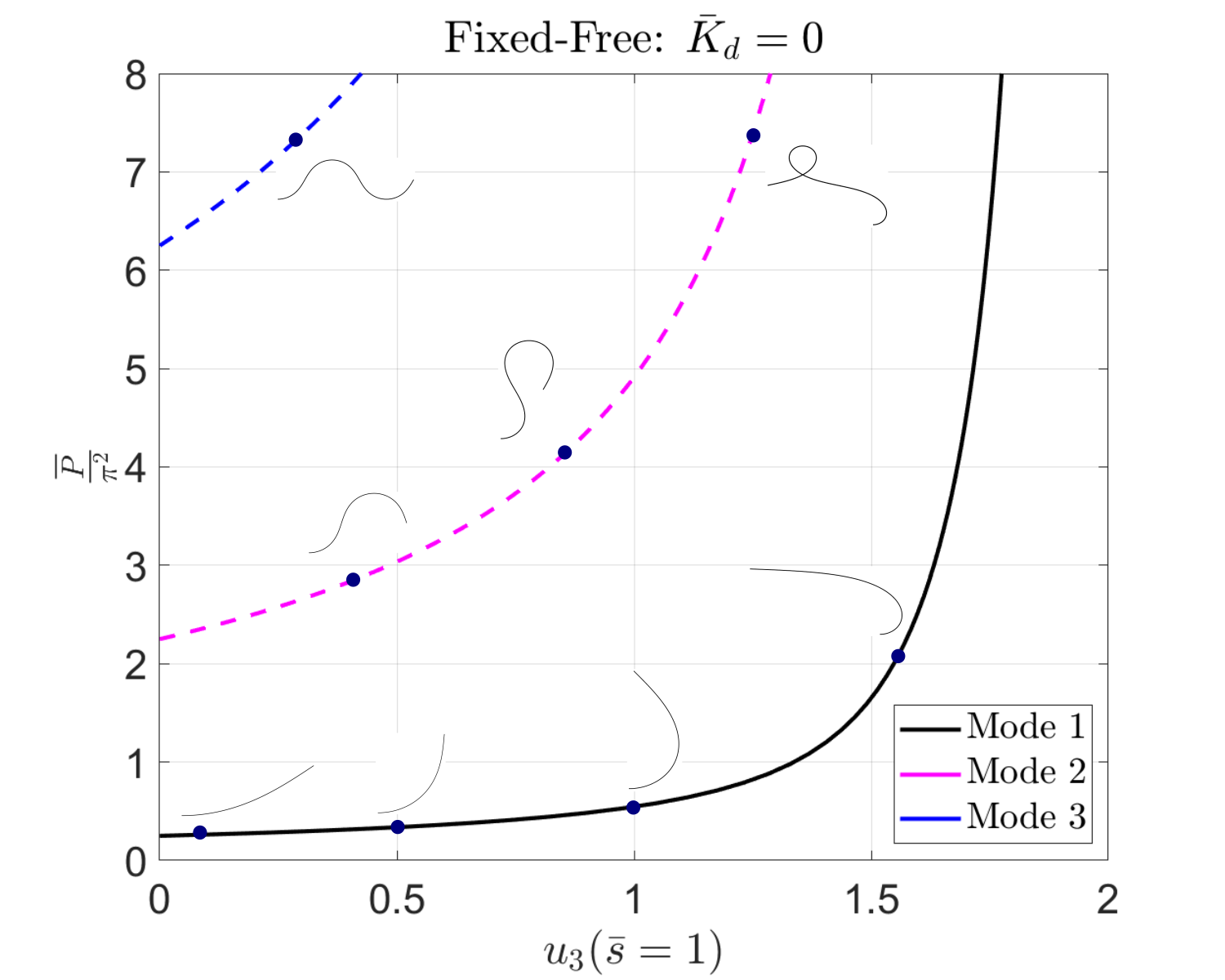
Fig. 7(a) shows the stability diagram for the first three nonlinear modes when the Elastica is fixed at one end while the other end remains free. We plot the horizontal displacement of the end-point, u3(s¯=1)=01cosθ(s¯)𝑑s¯subscript𝑢3¯𝑠1superscriptsubscript01𝜃¯𝑠differential-d¯𝑠u_{3}(\bar{s}=1)=\int_{0}^{1}\cos\theta(\bar{s})d\bar{s}, against loading parameter P¯¯𝑃\bar{P}. Note that P¯>0¯𝑃0\bar{P}>0 corresponds to compressive loads and P¯<0¯𝑃0\bar{P}<0 corresponds to tensile loads. The solid curves denote stable deformations while the dotted lines represent unstable deformations.
Refer to caption
(a)
Refer to caption
(b)
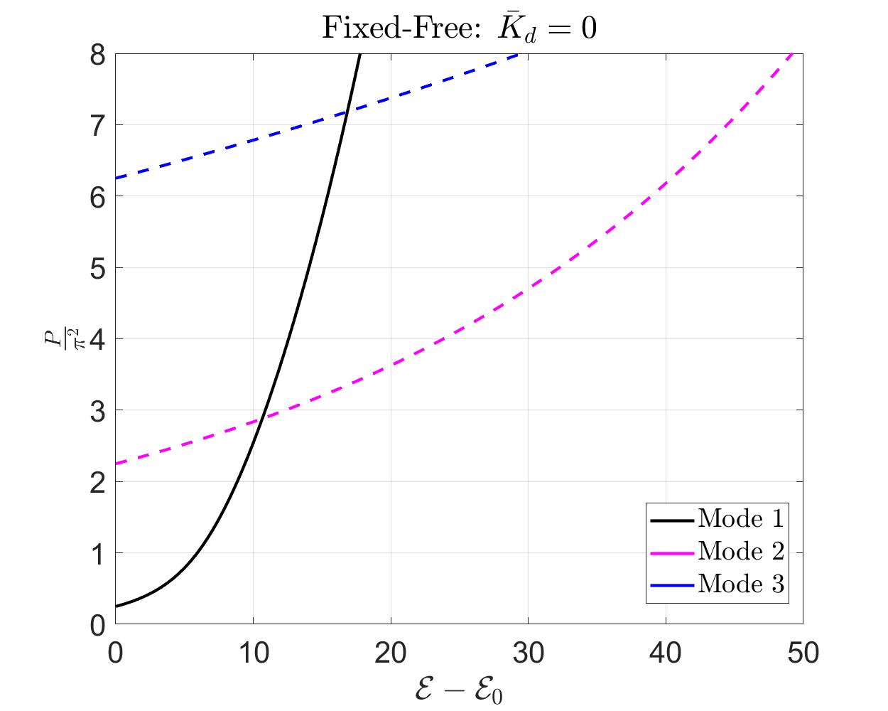
Figure 7: Euler’s Elastica: (a) Stability diagram, note that the first critical load is compressive, that is, P¯1=+π24subscript¯𝑃1superscript𝜋24\bar{P}_{1}=+\frac{\pi^{2}}{4}. (b) Total energy curve for fixed-free configuration; 0=0subscript00\mathcal{E}_{0}=0.

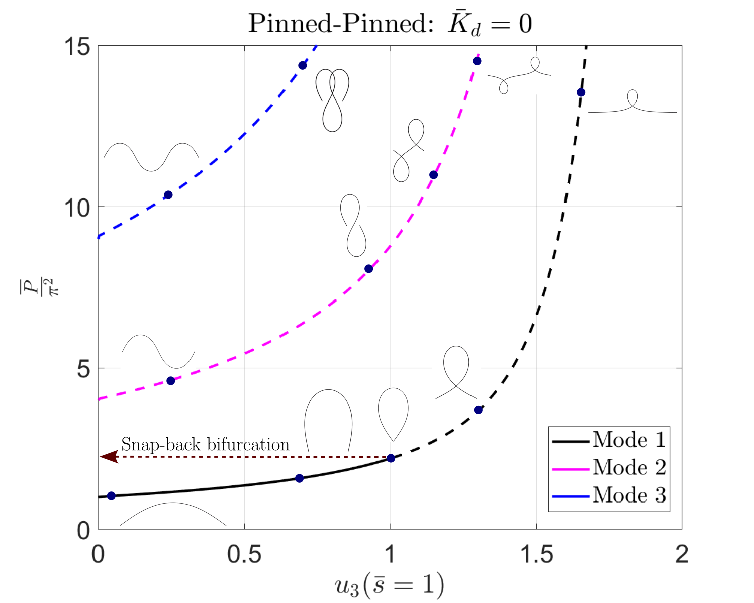
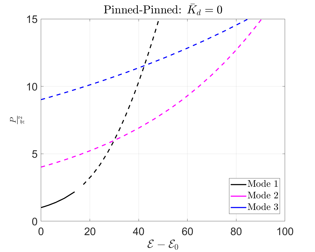
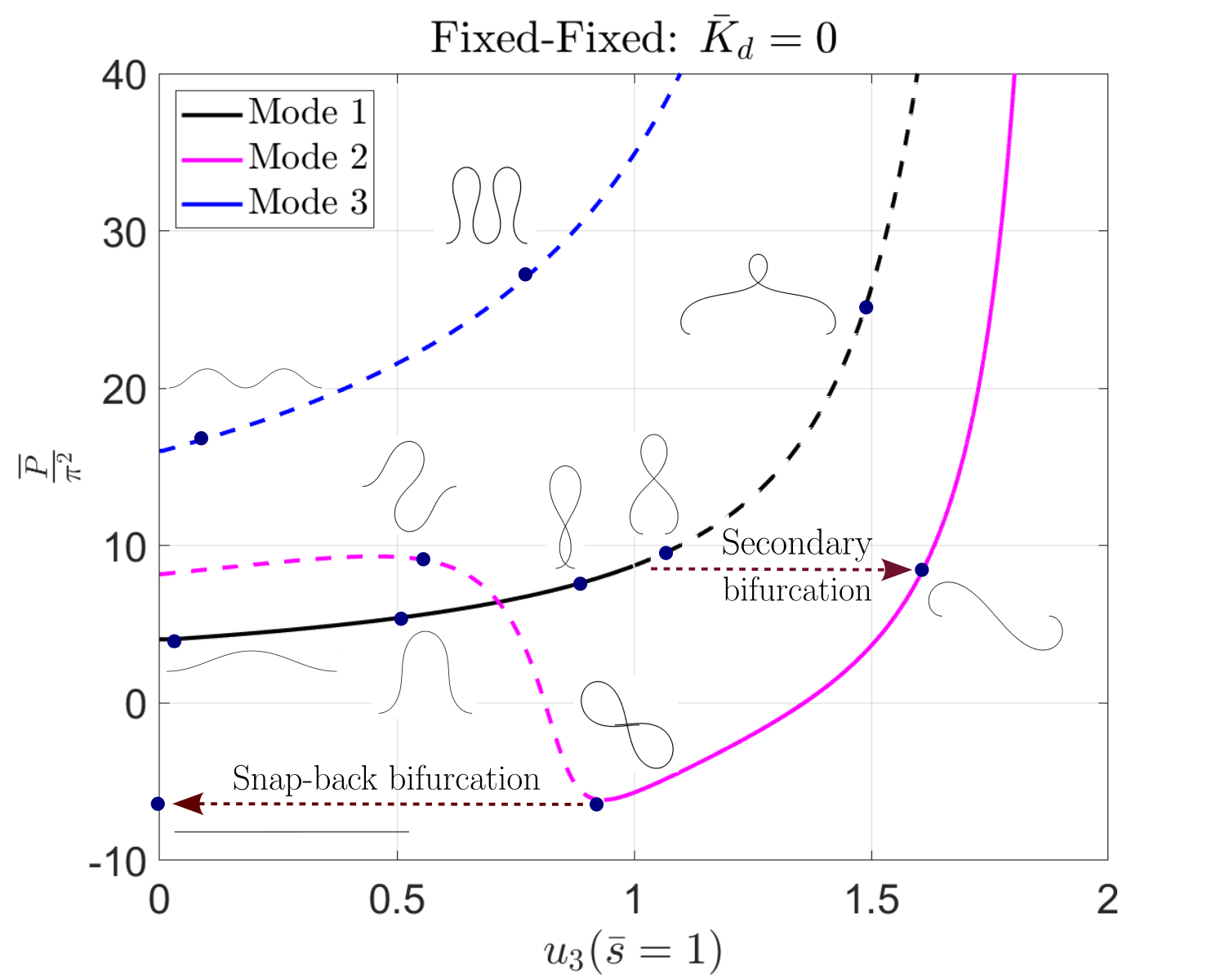
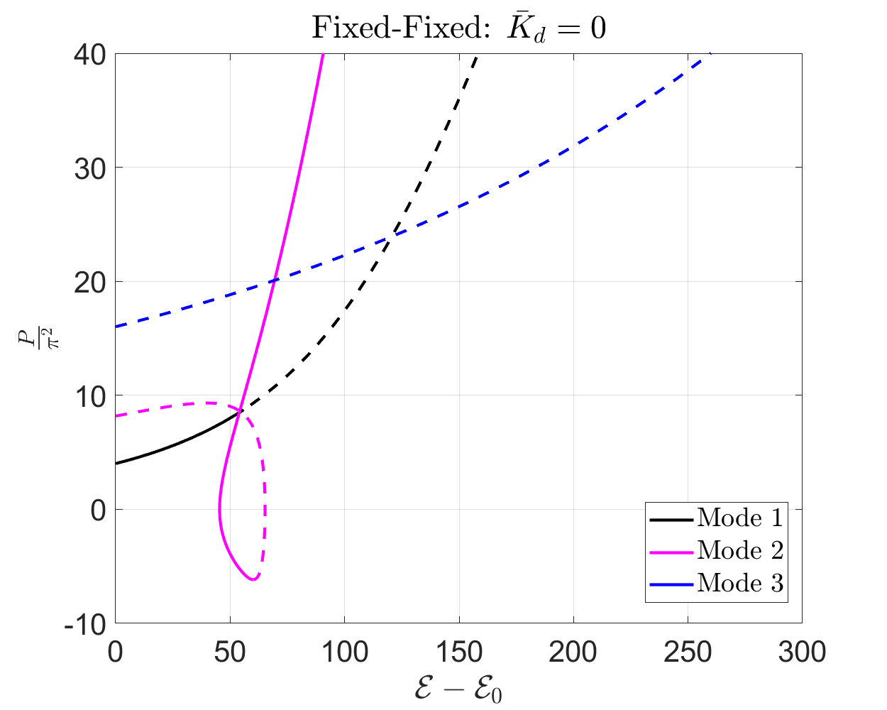
We observe that only the first nonlinear mode is stable. The stability diagram for the fixed-fixed scenario is shown in Fig. 8(a). We observe that the Elastica undergoes primary bifurcation along the first nonlinear mode initiating at the first critical P¯¯𝑃\bar{P} (obtained from linearized buckling analysis). The bifurcation at first critical P¯¯𝑃\bar{P} is continuous, as seen in Fig. 8(b). As P¯¯𝑃\bar{P} is increased beyond the first critical load, the two ends of the ribbon meet. Thereafter, it undergoes snap-through (secondary) bifurcation at P¯=10π2¯𝑃10superscript𝜋2\bar{P}=10\pi^{2} to the mode-2 branch. At the secondary bifurcation, the total energy of mode-1 becomes larger than that of mode-2, see Fig. 8. The ribbon continuous to deform on the second mode for P¯>10π2¯𝑃10superscript𝜋2\bar{P}>10\pi^{2}. If P¯¯𝑃\bar{P} is quasi-statically reduced along the mode-2 branch, the nature of buckling load gradually switches from compressive to tensile until it snap backs to the pre-buckled (reference) tensile configuration at P¯=6π2¯𝑃6superscript𝜋2\bar{P}=-6\pi^{2}. The stability diagram corresponding to pinned-pinned case (Fig. 9) shows that only mode-1 is the stable mode beyond the first critical load and it stays so till the end-points meet, after which the ribbon snaps to the pre-buckled (reference) configuration Levyakov2009 .
Refer to caption
(a)
Refer to caption
(b)
Figure 8: Euler’s Elastica: (a) Stability diagram (b) Total energy curve for fixed-fixed configuration; 0=0subscript00\mathcal{E}_{0}=0.
Refer to caption
(a)
Refer to caption
(b)
Figure 9: Euler’s Elastica: (a) Stability diagram (b) Total energy curve for pinned-pinned configuration; 0=0subscript00\mathcal{E}_{0}=0.

A close examination of Eqn. (27) reveals that under the transformation of θ𝜃\theta, i.e., θθ𝜃𝜃\theta\rightarrow-\theta, the equation possesses reflection symmetry if the condition R¯=0¯𝑅0\bar{R}=0 is met. We observe that R¯¯𝑅\bar{R} always remains zero for all P¯n(n=1,2,)subscript¯𝑃𝑛𝑛12\bar{P}_{n}\leavevmode\nobreak\ (n=1,2,\dots) for pinned-pinned scenario. Nevertheless, for the fixed-fixed case, R¯=0¯𝑅0\bar{R}=0 for odd n𝑛n (n=1,3,𝑛13n=1,3,\dots) while it is non-zero for even n𝑛n. The corresponding rich bifurcation behaviour in Fig. 8(a) could due attributed to this change of symmetry.

5.2 Soft ferromagnetic ribbon: Transverse external magnetic field, h¯e=𝒆2subscript¯𝑒subscript𝒆2\bar{h}_{e}={\bf\it e}_{2}

We recall the demag. energy in soft magnetic case is Kdat(𝒆2𝒏)2𝑑ssubscript𝐾𝑑𝑎𝑡superscriptsubscript𝒆2𝒏2differential-d𝑠K_{d}at\int({\bf\it e}_{2}\cdot{\bf\it n})^{2}ds. To minimize the demag. energy, the curve’s normal tends to align with the 𝒆3subscript𝒆3{\bf\it e}_{3} direction. This elongates the curve more in the 𝒆2subscript𝒆2{\bf\it e}_{2} direction. We consider K¯d=100subscript¯𝐾𝑑100\bar{K}_{d}=100 for our analysis, since the magnetostatic energy becomes comparable to the mechanical energy in this regime.

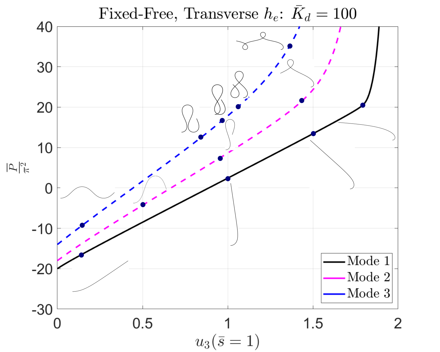
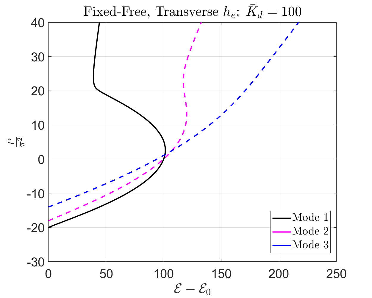
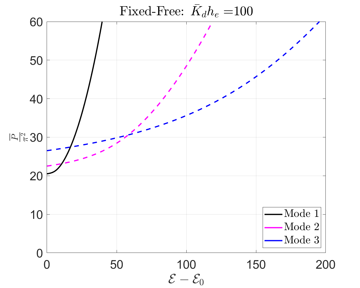
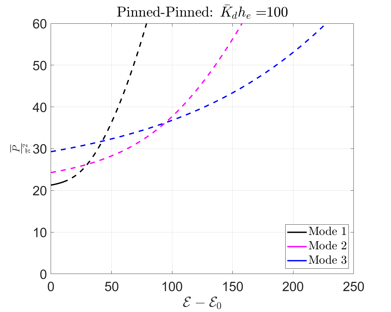
Fig. 10(a) shows the stability diagram for fixed-free boundary condition ferromagnetic ribbon in the presence of a transverse 𝒉esubscript𝒉𝑒{\bf\it h}_{e} external magnetic field, see Fig. 4. It is observed that the critical load here is tensile. The first nonlinear mode remains stable for all P¯>197.53¯𝑃197.53\bar{P}>-197.53 and this bifurcation is continuous.

Refer to caption
(a)
Refer to caption
(b)
Figure 10: Soft ferromagnetic ribbon, K¯d=100subscript¯𝐾𝑑100\bar{K}_{d}=100: (a) Stability diagram, note that the first critical load is tensile, that is, P¯1=20.01π2subscript¯𝑃120.01superscript𝜋2\bar{P}_{1}=-20.01\pi^{2}. (b) Total energy curve for fixed-free configuration under transverse magnetic field; 0=100subscript0100\mathcal{E}_{0}=-100.

For the fixed-fixed boundary condition, soft ferromagnetic ribbon buckles at a tensile load, and mode-1 deformation is observed for P¯>160.52¯𝑃160.52\bar{P}>-160.52, see Fig. 11. The ribbon snaps to the mode-2 branch as P¯¯𝑃\bar{P} is increased as seen in Fig. 11. The ribbon deforms further along the mode-2 branch with gradual decrease in P¯¯𝑃\bar{P}. As we unload, that is, decrease P¯¯𝑃\bar{P} on the mode-2 branch, we observe the formation of new stable deformed configurations for tensile loads before it snaps back to the reference state. We observe a prolonged stretch of a stable segment in the mode-2 branch under the influence of 𝒉esubscript𝒉𝑒{\bf\it h}_{e} for tensile loads (P¯<0¯𝑃0\bar{P}<0). This stable segment persists even after the two supports have crossed each other significantly. Interestingly, we observe novel and stable states in this segment of the mode-2 branch. This segment is highlighted in Fig. 11(a). We have highlighted one such novel and stable deformed configuration in red in Fig. 11(a), when the end displacement is u3=0.65subscript𝑢30.65u_{3}=0.65. Note that in the deformed configuration depicted in red in Fig. 11(a), there are two self-intersection points. A few intermediate novel deformed configurations are shown in red in Fig. 11(b). Curves with two self-intersection points are not observed in any stable configuration in the purely elastic case. As P¯¯𝑃\bar{P} is further reduced along this branch, that is, as we increase the tensile load, the ribbon undergoes a secondary bifurcation after which the ribbon snaps to the pre-buckled (reference) tensile configuration.
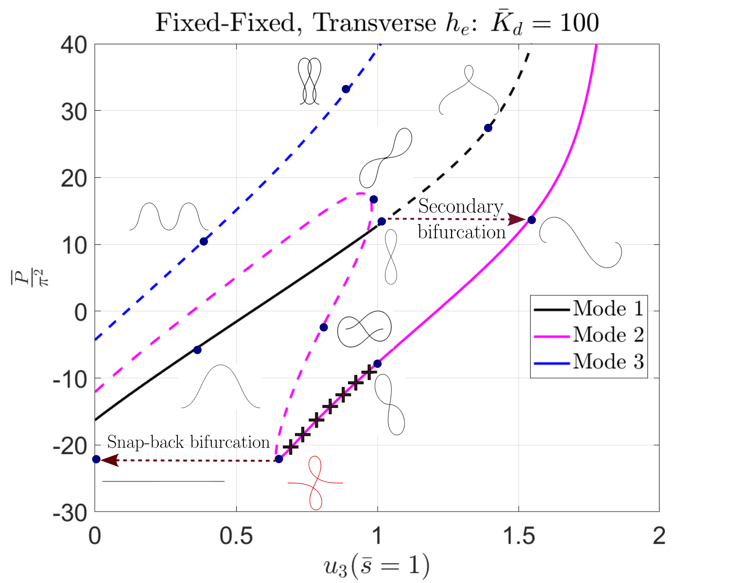
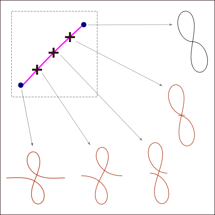
Refer to caption
(a)
Refer to caption
(b)
Refer to caption
(c)
Figure 11: Soft ferromagnetic ribbon, K¯d=100subscript¯𝐾𝑑100\bar{K}_{d}=100: (a) Stability diagram, segment of the mode-2 branch corresponding to novel stable curves is highlighted in ‘+’ symbol. Deformed config. shown in red represents one such novel stable curve on this segment that cannot be observed in purely elastic ribbon. (b) Segment of the mode-2 branch showing novel stable deformed configurations. (c) Total energy curve for fixed-fixed configuration under transverse magnetic field; 0=100subscript0100\mathcal{E}_{0}=-100.

For the pinned-pinned soft ferromagnetic ribbon, the stability diagram Fig. 12(a) is qualitatively similar to the purely elastic case, except that the deformed shape is elongated along the 𝒆2subscript𝒆2{\bf\it e}_{2} direction and the critical load is tensile. Thus, for a soft ferromagnetic ribbon for all the boundary conditions, the critical load is tensile and they can be determined from linearized equations (Eqn. (24)) about θ(s¯)0𝜃¯𝑠0\theta(\bar{s})\approx 0 such that sinθ(s¯)θ(s¯)𝜃¯𝑠𝜃¯𝑠\sin\theta(\bar{s})\approx\theta(\bar{s}) and cosθ(s¯)1𝜃¯𝑠1\cos\theta(\bar{s})\approx 1 as follows:

θ′′(s¯)+(P¯+2K¯d)θ(s¯)+R¯=0,superscript𝜃′′¯𝑠¯𝑃2subscript¯𝐾𝑑𝜃¯𝑠¯𝑅0\theta^{\prime\prime}(\bar{s})+(\bar{P}+2\bar{K}_{d})\theta(\bar{s})+\bar{R}=0, (74)

subject to the integral constraint (for fixed-fixed and pinned conditions):

y¯(1)=01θ(s¯)𝑑s¯=0,¯𝑦1superscriptsubscript01𝜃¯𝑠differential-d¯𝑠0\bar{y}(1)=\int_{0}^{1}\theta(\bar{s})\leavevmode\nobreak\ d\bar{s}=0,

and gives the critical loads as

  • fixed-free: P¯n=(n12)2π22K¯d,n=1,2,formulae-sequencesubscript¯𝑃𝑛superscript𝑛122superscript𝜋22subscript¯𝐾𝑑𝑛12\bar{P}_{n}=\left(n-\frac{1}{2}\right)^{2}\pi^{2}-2\bar{K}_{d},\quad n=1,2,\dots,

  • fixed-fixed: 2tanP¯n+2K¯d2=P¯n+2K¯d2subscript¯𝑃𝑛2subscript¯𝐾𝑑2subscript¯𝑃𝑛2subscript¯𝐾𝑑2\tan\frac{\sqrt{\bar{P}_{n}+2\bar{K}_{d}}}{2}=\sqrt{\bar{P}_{n}+2\bar{K}_{d}},

  • pinned-pinned: P¯n=n2π22K¯dsubscript¯𝑃𝑛superscript𝑛2superscript𝜋22subscript¯𝐾𝑑\bar{P}_{n}=n^{2}\pi^{2}-2\bar{K}_{d}.

Refer to caption
(a)
Refer to caption
(b)
Figure 12: Soft ferromagnetic ribbon, K¯d=100subscript¯𝐾𝑑100\bar{K}_{d}=100: (a) Stability diagram (b) Total energy curve for pinned-pinned configuration under transverse magnetic field; 0=100subscript0100\mathcal{E}_{0}=-100.

5.3 Hard ferromagnetic ribbon

We now present our analysis for the hard ferromagnetic ribbon. Recall that, in this case that the magnetization vector makes a constant angle with the tangent at each point along the curve. Comparing Eqns. (30) and (27) reveals that, in this case, magnetization does not change the structure of Euler’s Elastica equilibrium equations. The deformed configurations corresponding to the hard magnetic case are obtained by a simple translation of the stability curves of those of Euler’s Elastica (Figs. 7,8, 9) along P¯¯𝑃\bar{P}-axis, see Figs. 13, 14 and 15. It is also noted that the equations for the cases – axial 𝒉esubscript𝒉𝑒{\bf\it h}_{e}, 𝒎(s¯)=𝒕(s¯)𝒎¯𝑠𝒕¯𝑠{\bf\it m}(\bar{s})={\bf\it t}(\bar{s}) and transverse hesubscript𝑒h_{e}, 𝒎(s¯)=𝒏(s¯)𝒎¯𝑠𝒏¯𝑠{\bf\it m}(\bar{s})={\bf\it n}(\bar{s}) – coincide, thus leading to the same solutions. The critical loads significantly exceed those corresponding to the classical Elastica. This can easily be seen by linearizing Eqns. (30)1 and (30)4.

Our proposed model and results matches with the equilibrium equation for planar deformation of hard ferromagnetic ribbon under fixed-free configuration, as reported by Zhao et al Zhao2019 and Wang et al. Wang2020 ; Wang2022 , when only subjected to an external magnetic field and no mechanical load.

Axial external magnetic field hesubscript𝑒h_{e}

: Comparing equilibrium equation of the hard ferromagnetic ribbon with 𝒎(s¯)=𝒏(s¯)𝒎¯𝑠𝒏¯𝑠{\bf\it m}(\bar{s})={\bf\it n}(\bar{s}) (Eqn. (31)2) and Eqn. (27) shows that in this case

Q¯=R¯+2K¯dhe.¯𝑄¯𝑅2subscript¯𝐾𝑑subscript𝑒\bar{Q}=\bar{R}+2\bar{K}_{d}h_{e}. (75)

Thus, the results are identical.

Refer to caption
(a)
Refer to caption
(b)
Figure 13: Hard ferromagnetic ribbon: Axial hesubscript𝑒h_{e}, Fixed-Free, 𝒎=𝒕(s¯)𝒎𝒕¯𝑠{\bf\it m}={\bf\it t}(\bar{s}), K¯dhe=100subscript¯𝐾𝑑subscript𝑒100\bar{K}_{d}h_{e}=100: (a) Stability diagram (b) Total energy curve; 0=0subscript00\mathcal{E}_{0}=0.
Refer to caption
(a)
Refer to caption
(b)
Figure 14: Hard ferromagnetic ribbon: Axial hesubscript𝑒h_{e}, Fixed-Fixed, 𝒎=𝒕(s¯)𝒎𝒕¯𝑠{\bf\it m}={\bf\it t}(\bar{s}), K¯dhe=100subscript¯𝐾𝑑subscript𝑒100\bar{K}_{d}h_{e}=100: (a) Stability diagram (b) Total energy curve; 0=0subscript00\mathcal{E}_{0}=0.
Refer to caption
(a)
Refer to caption
(b)
Figure 15: Hard ferromagnetic ribbon: Axial hesubscript𝑒h_{e}, Pinned-Pinned, 𝒎=𝒕(s¯)𝒎𝒕¯𝑠{\bf\it m}={\bf\it t}(\bar{s}), K¯dhe=100subscript¯𝐾𝑑subscript𝑒100\bar{K}_{d}h_{e}=100: (a) Stability diagram (b) Total energy curve; 0=0subscript00\mathcal{E}_{0}=0.
Transverse external magnetic field hesubscript𝑒h_{e}

: The deformed configurations of the hard ferromagnetic ribbon with tangential magnetization distribution, 𝒎(s¯)=𝒕(s¯)𝒎¯𝑠𝒕¯𝑠{\bf\it m}(\bar{s})={\bf\it t}(\bar{s}), are identical to the purely elastic counterpart. On matching the coefficients of Eqns. (30)3 and (27), we arrrive at the following relationship between the Lagrange multipliers R¯¯𝑅\bar{R} and Q¯¯𝑄\bar{Q}:

Q¯=R¯2K¯dhe.¯𝑄¯𝑅2subscript¯𝐾𝑑subscript𝑒\bar{Q}=\bar{R}-2\bar{K}_{d}h_{e}. (76)

5.4 Limit as K¯dsubscript¯𝐾𝑑\bar{K}_{d}\rightarrow\infty

In this section, we explore the deformation of our planar ferromagnetic ribbons as the limit of K¯dsubscript¯𝐾𝑑\bar{K}_{d}\rightarrow\infty approaches infinity. This limit is also attained when E𝐸E, a𝑎a, l𝑙l, and Kdsubscript𝐾𝑑K_{d} are held constant, and as t0𝑡0t\rightarrow 0. This represents a physically relevant limit for nano rods/ribbons used in MEMS devices Samy2023 .

As K¯dsubscript¯𝐾𝑑\bar{K}_{d}\rightarrow\infty, the magnetostatic energy is much larger than the elastic energy. In this regime, the magnetization 𝒎𝒎{\bf\it m} and the normal 𝒏𝒏{\bf\it n} are perpendicular almost all along the length of the ribbon, except in short intervals where this condition cannot be met due to either the imposed mechanical boundary condition or due to the isoperimetric constraint imposed due to inextensibility. These short intervals exhibit a curvature with a radius denoted as rcsubscript𝑟𝑐r_{c}, see Fig. Fig. 16. An estimation of rcsubscript𝑟𝑐r_{c} can be obtained by balancing the elastic energy and demagnetization energy, as outlined below:

Total energy:EI20lκ2(s)𝑑s+Kdat0l(𝒎𝒏)2𝑑sEI02πr1r2𝑑s+Kdat02πr𝑑s=EI2πr+Kdat2πr.:Total energy𝐸𝐼2superscriptsubscript0𝑙superscript𝜅2𝑠differential-d𝑠subscript𝐾𝑑𝑎𝑡superscriptsubscript0𝑙superscript𝒎𝒏2differential-d𝑠𝐸𝐼superscriptsubscript02𝜋𝑟1superscript𝑟2differential-d𝑠subscript𝐾𝑑𝑎𝑡superscriptsubscript02𝜋𝑟differential-d𝑠𝐸𝐼2𝜋𝑟subscript𝐾𝑑𝑎𝑡2𝜋𝑟\begin{split}\text{Total energy}:&\quad\frac{EI}{2}\int_{0}^{l}\kappa^{2}(s)ds+K_{d}at\int_{0}^{l}({\bf\it m}\cdot{\bf\it n})^{2}ds\approx EI\int_{0}^{2\pi r}\frac{1}{r^{2}}ds+K_{d}at\int_{0}^{2\pi r}ds\\ &\qquad=\frac{EI\cdot 2\pi}{r}+K_{d}at\cdot 2\pi r.\end{split} (77)

Optimising the total energy with respect to r𝑟r, we obtain rc𝒪(tEKd)similar-tosubscript𝑟𝑐𝒪𝑡𝐸subscript𝐾𝑑r_{c}\sim\mathcal{O}\bigg{(}t\sqrt{\frac{E}{K_{d}}}\bigg{)}. The deformed configurations in this regime of fixed-free, fixed-fixed, and pinned-pinned soft ferromagnetic ribbons are shown in Figure 16.
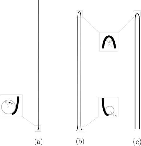
Refer to caption
Figure 16: Deformed shapes of soft ferromagnetic ribbon for K¯d=104subscript¯𝐾𝑑superscript104\bar{K}_{d}=10^{4} showing osculating circles at the curved bends: (a) fixed-free (b) fixed-fixed, and (c) pinned-pinned cases.

6 Conclusions

In this paper, we have presented a novel model that combines ideas from Euler’s Elastica and continuum theory of micromagnetics to predict the deformation of ferromagnetic ribbons. We have analysed the buckling of a planar inextensible ribbon subjected to a large but constant external magnetic field and a gradually applied quasi-static load. While maintaining fixed magnetisation, we investigate the influence of magnetisation on the deformation of the planar ferromagnetic ribbon. Exploring how deformation influences magnetisation is an intriguing area for future research, although it presents a challenging problem. Our analysis commences by deriving and incorporating the magnetostatic energy of a curved structure into the total energy of the system. We derive the equilibrium equations and solve them numerically to obtain the equilibrium path as the load is increased. Further, we also determine the stability of the equilibrium solutions by casting the second variation of the total energy as a Sturm-Liouville eigenvalue problem, which is solved numerically.

We examine ribbons composed of both hard and soft ferromagnetic properties, exploring different orientations of externally applied magnetic fields and various mechanical boundary conditions. We observe that the critical buckling load is tensile mainly for a soft ferromagnetic ribbon under various canonical boundary conditions. Interestingly, our findings reveal the presence of novel stable configurations in the case of a fixed-fixed setup with a transversally applied external magnetic field. We anticipate that these stable configurations can be observed through meticulously conducted experiments.

Our analysis can be readily extended to understanding the deformation of planar ferromagnetic rods. The magnetostatic energy of planar ferromagnetic rod scales as 𝒪(Kdπr2l)𝒪subscript𝐾𝑑𝜋superscript𝑟2𝑙\mathcal{O}(K_{d}\pi r^{2}l) Slastikov2011 . A balance of the elastic energy 𝒪(Eπ(r48l))𝒪𝐸𝜋superscript𝑟48𝑙\mathcal{O}(E\pi\big{(}\frac{r^{4}}{8l})\big{)}, and the magnetostatic energy for ferromagnetic rods would suggest that our analysis remains valid for rods with an aspect ratio of 𝒪(E8Kd)𝒪𝐸8𝐾𝑑\mathcal{O}\bigg{(}\sqrt{\frac{E}{8Kd}}\bigg{)}.

The stability analysis conducted in our study solely examines planar perturbations. It is widely recognized that, in the case of Euler’s Elastica, stability under planar perturbations does not guarantee stability of the equilibrium configurations under fully three-dimensional perturbations Maddocks1984 . Motivated by this study, we outline the following future research directions:

\bullet 

Explore stability under three-dimensional perturbations, and ascertain the potential role of the vertical reaction, R¯¯𝑅\bar{R}, in this analysis.

\bullet 

Investigating the influence of twist and out-of-plane deformation on ferromagnetic ribbons.

\bullet 

Design laboratory experiments to observe novel stable deformed configurations of ferromagnetic ribbon structures, as identified in our analysis.

Acknowledgements.
We acknowledge Dr. Raghavendra Venkatraman (Courant Institute) for his valuable suggestions and insights on the draft of this paper. Furthermore, we would like to acknowledge the Indian Institute of Science Startup Grant and the Prime Minister’s Research Fellowship (PMRF ID: 0201857) for providing financial support for this research.

Conflict of interest

The authors declare that they have no conflict of interest.

Appendix A Derivation of magnetostatic energy

In this section, we present the calculation of the leading order demag. energy of a deformed planar ferromagnetic ribbon. The magnetostatic energy is evaluated by solving Maxwell’s equations of magnetostatics

×𝒉m(𝒙)=0,(𝒉m+𝒎(𝒙))=0.formulae-sequencesubscript𝒉𝑚𝒙0subscript𝒉𝑚𝒎𝒙0\begin{split}\curl{{\bf\it h}_{m}({\bf\it x})}&=0,\\ \divergence({\bf\it h}_{m}+{\bf\it m}({\bf\it x}))&=0.\end{split} (78)

Applying Fourier transform to the above equations imply

𝝃×𝒉^mcross-product𝝃subscript^𝒉𝑚\displaystyle{\bf\it\xi}\crossproduct\hat{{\bf\it h}}_{m} =0,absent0\displaystyle=0, (79)
𝝃(𝒉^m+𝒎^)𝝃subscript^𝒉𝑚^𝒎\displaystyle{\bf\it\xi}\cdot(\hat{{\bf\it h}}_{m}+\hat{{\bf\it m}}) =0,absent0\displaystyle=0, (80)

where 𝒇^(𝝃):=3𝒇(𝒙)exp(i2π𝒙𝝃)𝑑𝒙assign^𝒇𝝃subscriptsuperscript3𝒇𝒙𝑖2𝜋𝒙𝝃differential-d𝒙\hat{{\bf\it f}}({\bf\it\xi}):=\int_{\mathbb{R}^{3}}{\bf\it f}({\bf\it x})\exp(-i2\pi{\bf\it x}\cdot{\bf\it\xi})d{\bf\it x}. Eqn. (79) implies 𝒉^m𝝃conditionalsubscript^𝒉𝑚𝝃\hat{{\bf\it h}}_{m}\parallel{\bf\it\xi} and hence,

𝒉^m=(𝒉^m𝝃^)𝝃^ where 𝝃^=𝝃|𝝃|.subscript^𝒉𝑚subscript^𝒉𝑚^𝝃^𝝃 where ^𝝃𝝃𝝃\hat{{\bf\it h}}_{m}=(\hat{{\bf\it h}}_{m}\cdot\hat{{\bf\it\xi}})\hat{{\bf\it\xi}}\text{ where }\hat{{\bf\it\xi}}=\frac{{\bf\it\xi}}{\absolutevalue{{\bf\it\xi}}}. (81)

Eqn. (80) implies that 𝝃𝒉^m=𝝃𝒎^𝝃subscript^𝒉𝑚𝝃^𝒎{\bf\it\xi}\cdot\hat{{\bf\it h}}_{m}=-{\bf\it\xi}\cdot\hat{{\bf\it m}} and hence 𝒉^m=(𝝃^𝒎^)𝝃^subscript^𝒉𝑚^𝝃^𝒎^𝝃\hat{{\bf\it h}}_{m}=-(\hat{{\bf\it\xi}}\cdot\hat{{\bf\it m}})\hat{{\bf\it\xi}}. Using Planchevel’s identity, we can then write the magnetostatic energy as follows

3|𝒉m|2𝑑𝒙=3|𝒉^m|2𝑑𝝃=3(𝝃^𝒎^)2𝑑𝝃=3(𝝃𝒎^)2|𝝃|2𝑑𝝃=3|𝒎^|2|𝝃|2𝑑𝝃.subscriptsuperscript3superscriptsubscript𝒉𝑚2differential-d𝒙subscriptsuperscript3superscriptsubscript^𝒉𝑚2differential-d𝝃subscriptsuperscript3superscript^𝝃^𝒎2differential-d𝝃subscriptsuperscript3superscript𝝃^𝒎2superscript𝝃2differential-d𝝃subscriptsuperscript3superscript^𝒎2superscript𝝃2differential-d𝝃\int_{\mathbb{R}^{3}}\absolutevalue{{\bf\it h}_{m}}^{2}d{\bf\it x}=\int_{\mathbb{R}^{3}}\absolutevalue{\hat{{\bf\it h}}_{m}}^{2}d{\bf\it\xi}=\int_{\mathbb{R}^{3}}(\hat{{\bf\it\xi}}\cdot\hat{{\bf\it m}})^{2}d{\bf\it\xi}=\int_{\mathbb{R}^{3}}\frac{({\bf\it\xi}\cdot\hat{{\bf\it m}})^{2}}{\absolutevalue{{\bf\it\xi}}^{2}}d{\bf\it\xi}=\int_{\mathbb{R}^{3}}\frac{\absolutevalue{\widehat{\divergence{\bf\it m}}}^{2}}{\absolutevalue{{\bf\it\xi}}^{2}}d{\bf\it\xi}. (82)

We carry out the above integration in the material frame (𝒅1(s),𝒅2(s),𝒅3(s))subscript𝒅1𝑠subscript𝒅2𝑠subscript𝒅3𝑠({\bf\it d}_{1}(s),{\bf\it d}_{2}(s),{\bf\it d}_{3}(s)) and 𝒙𝒓(s)+a~𝒅1(s)+t~𝒅2(s)maps-to𝒙𝒓𝑠~𝑎subscript𝒅1𝑠~𝑡subscript𝒅2𝑠{\bf\it x}\mapsto{\bf\it r}(s)+\tilde{a}{\bf\it d}_{1}(s)+\tilde{t}{\bf\it d}_{2}(s). The Fourier transform in the material frame is given as follows:

[𝒎](𝝃)=𝒎^(𝝃)=Ω(𝒎)exp(i2π𝒙𝝃)𝑑𝒙=Ω(𝒎)exp(i2π(𝒓(s)+a~𝒅1(s)+t~𝒅2(s))𝝃)J𝑑s𝑑t~𝑑a~,delimited-[]𝒎𝝃^𝒎𝝃subscriptΩ𝒎𝑖2𝜋𝒙𝝃differential-d𝒙subscriptΩ𝒎𝑖2𝜋𝒓𝑠~𝑎subscript𝒅1𝑠~𝑡subscript𝒅2𝑠𝝃𝐽differential-d𝑠differential-d~𝑡differential-d~𝑎\mathcal{F}[\divergence{\bf\it m}]({\bf\it\xi})=\widehat{\divergence{\bf\it m}}({\bf\it\xi})=\int_{\Omega}(\divergence{\bf\it m})\exp(-i2\pi{\bf\it x}\cdot{\bf\it\xi})d{\bf\it x}=\int_{\Omega}(\divergence{\bf\it m})\exp(-i2\pi({\bf\it r}(s)+\tilde{a}{\bf\it d}_{1}(s)+\tilde{t}{\bf\it d}_{2}(s))\cdot{\bf\it\xi})Jdsd\tilde{t}d\tilde{a}, (83)

here, (v)𝑣\mathcal{F}(v) denotes Fourier transform of v𝑣v and J=|(x1,x2,x3)(s,a~,t~)|𝐽subscript𝑥1subscript𝑥2subscript𝑥3𝑠~𝑎~𝑡J=\absolutevalue{\frac{\partial(x_{1},x_{2},x_{3})}{\partial(s,\tilde{a},\tilde{t})}} is the Jacobian associated with the change of variables. The divergence of 𝒎𝒎{\bf\it m} is invariant upon coordinate transformation and is expressed as follows in the material frame:

𝒎=1hsha~ht~{(ha~ht~md3)s+(ht~hsmd1)a~+(hsha~md2)t~},𝒎1subscript𝑠subscript~𝑎subscript~𝑡partial-derivative𝑠subscript~𝑎subscript~𝑡subscript𝑚subscript𝑑3partial-derivative~𝑎subscript~𝑡subscript𝑠subscript𝑚subscript𝑑1partial-derivative~𝑡subscript𝑠subscript~𝑎subscript𝑚subscript𝑑2\divergence{\bf\it m}=\frac{1}{h_{s}h_{\tilde{a}}h_{\tilde{t}}}\left\{\partialderivative{(h_{\tilde{a}}h_{\tilde{t}}m_{d_{3}})}{s}+\partialderivative{(h_{\tilde{t}}h_{s}m_{d_{1}})}{\tilde{a}}+\partialderivative{(h_{s}h_{\tilde{a}}m_{d_{2}})}{\tilde{t}}\right\}, (84)

here, hs=|𝒙s|,ha~=|𝒙a~|formulae-sequencesubscript𝑠partial-derivative𝑠𝒙subscript~𝑎partial-derivative~𝑎𝒙h_{s}=\absolutevalue{\partialderivative{{\bf\it x}}{s}},h_{\tilde{a}}=\absolutevalue{\partialderivative{{\bf\it x}}{\tilde{a}}} and ht~=|𝒙t~|subscript~𝑡partial-derivative~𝑡𝒙h_{\tilde{t}}=\absolutevalue{\partialderivative{{\bf\it x}}{\tilde{t}}}.
Note:

  • 𝒙s=𝒓(s)+a~𝒅1(s)+t~𝒅2(s)=𝒅3(s)+t~κ𝒅3(s)=(1+t~κ)𝒅3(s)hs=(1+t~κ)partial-derivative𝑠𝒙superscript𝒓𝑠~𝑎superscriptsubscript𝒅1𝑠~𝑡superscriptsubscript𝒅2𝑠subscript𝒅3𝑠~𝑡𝜅subscript𝒅3𝑠1~𝑡𝜅subscript𝒅3𝑠subscript𝑠1~𝑡𝜅\partialderivative{{\bf\it x}}{s}={\bf\it r}^{\prime}(s)+\tilde{a}{\bf\it d}_{1}^{\prime}(s)+\tilde{t}{\bf\it d}_{2}^{\prime}(s)={\bf\it d}_{3}(s)+\tilde{t}\kappa{\bf\it d}_{3}(s)=(1+\tilde{t}\kappa){\bf\it d}_{3}(s)\implies h_{s}=(1+\tilde{t}\kappa),

  • 𝒙a~=𝒅1(s)ha~=1partial-derivative~𝑎𝒙subscript𝒅1𝑠subscript~𝑎1\partialderivative{{\bf\it x}}{\tilde{a}}={\bf\it d}_{1}(s)\implies h_{\tilde{a}}=1,

  • 𝒙t~=𝒅2(s)ht~=1partial-derivative~𝑡𝒙subscript𝒅2𝑠subscript~𝑡1\partialderivative{{\bf\it x}}{\tilde{t}}={\bf\it d}_{2}(s)\implies h_{\tilde{t}}=1.

Furthermore, J=hsha~ht~𝐽subscript𝑠subscript~𝑎subscript~𝑡J=h_{s}h_{\tilde{a}}h_{\tilde{t}}, and hence

𝒎𝒎\displaystyle\divergence{\bf\it m} =1J{md3s+(1+t~κ)md1a~+(1+t~κ)md2t~+κmd2}absent1𝐽partial-derivative𝑠subscript𝑚subscript𝑑31~𝑡𝜅partial-derivative~𝑎subscript𝑚subscript𝑑11~𝑡𝜅partial-derivative~𝑡subscript𝑚subscript𝑑2𝜅subscript𝑚subscript𝑑2\displaystyle=\frac{1}{J}\left\{\partialderivative{m_{d_{3}}}{s}+(1+\tilde{t}\kappa)\partialderivative{m_{d_{1}}}{\tilde{a}}+(1+\tilde{t}\kappa)\partialderivative{m_{d_{2}}}{\tilde{t}}+\kappa m_{d_{2}}\right\}
=1J{(a~md1+t~md2+smd3)+κ(t~a~md1+t~t~md2+md2)}.absent1𝐽subscript~𝑎subscript𝑚subscript𝑑1subscript~𝑡subscript𝑚subscript𝑑2subscript𝑠subscript𝑚subscript𝑑3𝜅~𝑡subscript~𝑎subscript𝑚subscript𝑑1~𝑡subscript~𝑡subscript𝑚subscript𝑑2subscript𝑚subscript𝑑2\displaystyle=\frac{1}{J}\left\{(\partial_{\tilde{a}}m_{d_{1}}+\partial_{\tilde{t}}m_{d_{2}}+\partial_{s}m_{d_{3}})+\kappa(\tilde{t}\partial_{\tilde{a}}m_{d_{1}}+\tilde{t}\partial_{\tilde{t}}m_{d_{2}}+m_{d_{2}})\right\}. (85)

Substituting the above expression for 𝒎𝒎\divergence{\bf\it m} in Eqn. (83) can now be written as follows:

[𝒎](𝝃)=Ω1J{(a~md1+t~md2+smd3)+κ(t~a~md1+t~t~md2+md2)}exp(i2π(𝒓(s)+a~𝒅1(s)+t~𝒅2(s))𝝃)J𝑑s𝑑t~𝑑a~.delimited-[]𝒎𝝃subscriptΩ1𝐽subscript~𝑎subscript𝑚subscript𝑑1subscript~𝑡subscript𝑚subscript𝑑2subscript𝑠subscript𝑚subscript𝑑3𝜅~𝑡subscript~𝑎subscript𝑚subscript𝑑1~𝑡subscript~𝑡subscript𝑚subscript𝑑2subscript𝑚subscript𝑑2𝑖2𝜋𝒓𝑠~𝑎subscript𝒅1𝑠~𝑡subscript𝒅2𝑠𝝃𝐽differential-d𝑠differential-d~𝑡differential-d~𝑎\mathcal{F}[\divergence{\bf\it m}]({\bf\it\xi})=\int_{\Omega}\frac{1}{J}\left\{(\partial_{\tilde{a}}m_{d_{1}}+\partial_{\tilde{t}}m_{d_{2}}+\partial_{s}m_{d_{3}})+\kappa(\tilde{t}\partial_{\tilde{a}}m_{d_{1}}+\tilde{t}\partial_{\tilde{t}}m_{d_{2}}+m_{d_{2}})\right\}\exp(-i2\pi({\bf\it r}(s)+\tilde{a}{\bf\it d}_{1}(s)+\tilde{t}{\bf\it d}_{2}(s))\cdot{\bf\it\xi})Jdsd\tilde{t}d\tilde{a}. (86)

Since 𝒓(0)=0𝒓0bold-italic-0{\bf\it r}(0)={\bf\it 0} and 𝒓(s)𝝃=0s𝒅3(s)𝑑s𝝃=sξd3𝒓𝑠𝝃superscriptsubscript0𝑠subscript𝒅3superscript𝑠differential-dsuperscript𝑠𝝃𝑠subscript𝜉subscript𝑑3{\bf\it r}(s)\cdot{\bf\it\xi}=\int_{0}^{s}{\bf\it d}_{3}(s^{\prime})ds^{\prime}\cdot{\bf\it\xi}=s\xi_{d_{3}} and therefore, (𝒓(s)+a~𝒅1(s)+t~𝒅2(s))𝝃=a~ξd1+t~ξd2+sξd3𝒓𝑠~𝑎subscript𝒅1𝑠~𝑡subscript𝒅2𝑠𝝃~𝑎subscript𝜉subscript𝑑1~𝑡subscript𝜉subscript𝑑2𝑠subscript𝜉subscript𝑑3({\bf\it r}(s)+\tilde{a}{\bf\it d}_{1}(s)+\tilde{t}{\bf\it d}_{2}(s))\cdot{\bf\it\xi}=\tilde{a}\xi_{d_{1}}+\tilde{t}\xi_{d_{2}}+s\xi_{d_{3}}. The divergence of 𝒎𝒎{\bf\it m} in the material frame is written as a sum of these six integrals:

[𝒎](𝝃)=I1+I2+I3+I4+I5+I6,delimited-[]𝒎𝝃subscript𝐼1subscript𝐼2subscript𝐼3subscript𝐼4subscript𝐼5subscript𝐼6\mathcal{F}[\divergence{\bf\it m}]({\bf\it\xi})=I_{1}+I_{2}+I_{3}+I_{4}+I_{5}+I_{6}, (87)

where

I1=[a~md1](𝝃d)=ξd1F0(a,ξd1)F0(t,ξd2)[md1χ(0,l)(s)](ξd3)(even in ξd2),I2=[t~md2](𝝃d)=ξd2F0(a,ξd1)F0(t,ξd2)[md2χ(0,l)(s)](ξd3)(odd in ξd2),I3=[smd3](𝝃d)=F0(a,ξd1)F0(t,ξd2)[smd3χ(0,l)(s)](ξd3)(even in ξd2),I4=[κt~a~md1](𝝃d)=ξd1F0(a,ξd1)F1(t,ξd2)[κmd1χ(0,l)(s)](ξd3)(odd in ξd2),I5=[κt~t~md2](𝝃d)=F0(a,ξd1)ξd2F1(t,ξd2)[κmd2χ(0,l)(s)](ξd3)(even in ξd2),I6=[κmd2](𝝃d)=F0(a,ξd1)F1(t,ξd2)[κmd2χ(0,l)(s)](ξd3)(even in ξd2),formulae-sequencesubscript𝐼1delimited-[]subscript~𝑎subscript𝑚subscript𝑑1subscript𝝃𝑑subscript𝜉subscript𝑑1subscript𝐹0𝑎subscript𝜉subscript𝑑1subscript𝐹0𝑡subscript𝜉subscript𝑑2delimited-[]subscript𝑚subscript𝑑1subscript𝜒0𝑙𝑠subscript𝜉subscript𝑑3(even in ξd2)subscript𝐼2delimited-[]subscript~𝑡subscript𝑚subscript𝑑2subscript𝝃𝑑subscript𝜉subscript𝑑2subscript𝐹0𝑎subscript𝜉subscript𝑑1subscript𝐹0𝑡subscript𝜉subscript𝑑2delimited-[]subscript𝑚subscript𝑑2subscript𝜒0𝑙𝑠subscript𝜉subscript𝑑3(odd in ξd2)subscript𝐼3delimited-[]subscript𝑠subscript𝑚subscript𝑑3subscript𝝃𝑑subscript𝐹0𝑎subscript𝜉subscript𝑑1subscript𝐹0𝑡subscript𝜉subscript𝑑2delimited-[]subscript𝑠subscript𝑚subscript𝑑3subscript𝜒0𝑙𝑠subscript𝜉subscript𝑑3(even in ξd2)subscript𝐼4delimited-[]𝜅~𝑡subscript~𝑎subscript𝑚subscript𝑑1subscript𝝃𝑑subscript𝜉subscript𝑑1subscript𝐹0𝑎subscript𝜉subscript𝑑1subscript𝐹1𝑡subscript𝜉subscript𝑑2delimited-[]𝜅subscript𝑚subscript𝑑1subscript𝜒0𝑙𝑠subscript𝜉subscript𝑑3(odd in ξd2)subscript𝐼5delimited-[]𝜅~𝑡subscript~𝑡subscript𝑚subscript𝑑2subscript𝝃𝑑subscript𝐹0𝑎subscript𝜉subscript𝑑1subscript𝜉subscript𝑑2subscript𝐹1𝑡subscript𝜉subscript𝑑2delimited-[]𝜅subscript𝑚subscript𝑑2subscript𝜒0𝑙𝑠subscript𝜉subscript𝑑3(even in ξd2)subscript𝐼6delimited-[]𝜅subscript𝑚subscript𝑑2subscript𝝃𝑑subscript𝐹0𝑎subscript𝜉subscript𝑑1subscript𝐹1𝑡subscript𝜉subscript𝑑2delimited-[]𝜅subscript𝑚subscript𝑑2subscript𝜒0𝑙𝑠subscript𝜉subscript𝑑3(even in ξd2)\begin{split}I_{1}&=\mathcal{F}[\partial_{\tilde{a}}m_{d_{1}}]({\bf\it\xi}_{d})=\xi_{d_{1}}F_{0}(a,\xi_{d_{1}})F_{0}(t,\xi_{d_{2}})\mathcal{F}[m_{d_{1}}\chi_{(0,l)}(s)](\xi_{d_{3}})\quad\text{(even in $\xi_{d_{2}}$)},\\ I_{2}&=\mathcal{F}[\partial_{\tilde{t}}m_{d_{2}}]({\bf\it\xi}_{d})=\xi_{d_{2}}F_{0}(a,\xi_{d_{1}})F_{0}(t,\xi_{d_{2}})\mathcal{F}[m_{d_{2}}\chi_{(0,l)}(s)](\xi_{d_{3}})\quad\text{(odd in $\xi_{d_{2}}$)},\\ I_{3}&=\mathcal{F}[\partial_{s}m_{d_{3}}]({\bf\it\xi}_{d})=F_{0}(a,\xi_{d_{1}})F_{0}(t,\xi_{d_{2}})\mathcal{F}[\partial_{s}m_{d_{3}}\chi_{(0,l)}(s)](\xi_{d_{3}})\quad\text{(even in $\xi_{d_{2}}$)},\\ I_{4}&=\mathcal{F}[\kappa\tilde{t}\partial_{\tilde{a}}m_{d_{1}}]({\bf\it\xi}_{d})=\xi_{d_{1}}F_{0}(a,\xi_{d_{1}})F_{1}(t,\xi_{d_{2}})\mathcal{F}[\kappa m_{d_{1}}\chi_{(0,l)}(s)](\xi_{d_{3}})\quad\text{(odd in $\xi_{d_{2}}$)},\\ I_{5}&=\mathcal{F}[\kappa\tilde{t}\partial_{\tilde{t}}m_{d_{2}}]({\bf\it\xi}_{d})=F_{0}(a,\xi_{d_{1}})\xi_{d_{2}}F_{1}(t,\xi_{d_{2}})\mathcal{F}[\kappa m_{d_{2}}\chi_{(0,l)}(s)](\xi_{d_{3}})\quad\text{(even in $\xi_{d_{2}}$)},\\ I_{6}&=\mathcal{F}[\kappa m_{d_{2}}]({\bf\it\xi}_{d})=F_{0}(a,\xi_{d_{1}})F_{1}(t,\xi_{d_{2}})\mathcal{F}[\kappa m_{d_{2}}\chi_{(0,l)}(s)](\xi_{d_{3}})\quad\text{(even in $\xi_{d_{2}}$)},\end{split} (88)

where F0(v,η)subscript𝐹0𝑣𝜂F_{0}(v,\eta) and F1(v,η)subscript𝐹1𝑣𝜂F_{1}(v,\eta) are defined as follows:

F0(v,η)=v/2v/2exp(i2πηv)𝑑v and F1(v,η)=v/2v/2vexp(i2πηv)𝑑v.formulae-sequencesubscript𝐹0𝑣𝜂superscriptsubscript𝑣2𝑣2𝑖2𝜋𝜂superscript𝑣differential-dsuperscript𝑣 and subscript𝐹1𝑣𝜂superscriptsubscript𝑣2𝑣2superscript𝑣𝑖2𝜋𝜂superscript𝑣differential-dsuperscript𝑣F_{0}(v,\eta)=\int_{-v/2}^{v/2}\exp(-i2\pi\eta v^{\prime})dv^{\prime}\quad\text{ and }\quad F_{1}(v,\eta)=\int_{-v/2}^{v/2}v^{\prime}\exp(-i2\pi\eta v^{\prime})dv^{\prime}.

The magnetostatic energy can now be expressed in terms of I1,I2,I3,I4,I5,I6subscript𝐼1subscript𝐼2subscript𝐼3subscript𝐼4subscript𝐼5subscript𝐼6I_{1},I_{2},I_{3},I_{4},I_{5},I_{6} as follows:

3|𝒎^(𝝃d)|2|𝝃d|2𝑑𝝃d=3(I1+I2+I3+I4+I5+I6)2|𝝃d|2=I12|𝝃d|2𝒪(t2)+I22|𝝃d|2𝒪(t)+I32|𝝃d|2𝒪(t2)+I42|𝝃d|2𝒪(t5)+I52|𝝃d|2𝒪(t3)+I62|𝝃d|2𝒪(t3)+2I1I3|𝝃d|2𝒪(t2)+2I1I5|𝝃d|2𝒪(t3)+2I1I6|𝝃d|2𝒪(t2)+2I2I4|𝝃d|2𝒪(t3)+2I3I5|𝝃d|2𝒪(t3)+2I3I6|𝝃d|2𝒪(t2)+2I5I6|𝝃d|2𝒪(t3).subscriptsuperscript3superscript^𝒎subscript𝝃𝑑2superscriptsubscript𝝃𝑑2differential-dsubscript𝝃𝑑subscriptsuperscript3superscriptsubscript𝐼1subscript𝐼2subscript𝐼3subscript𝐼4subscript𝐼5subscript𝐼62superscriptsubscript𝝃𝑑2subscriptsuperscriptsubscript𝐼12superscriptsubscript𝝃𝑑2𝒪superscript𝑡2subscriptsuperscriptsubscript𝐼22superscriptsubscript𝝃𝑑2𝒪𝑡subscriptsuperscriptsubscript𝐼32superscriptsubscript𝝃𝑑2𝒪superscript𝑡2subscriptsuperscriptsubscript𝐼42superscriptsubscript𝝃𝑑2𝒪superscript𝑡5subscriptsuperscriptsubscript𝐼52superscriptsubscript𝝃𝑑2𝒪superscript𝑡3subscriptsuperscriptsubscript𝐼62superscriptsubscript𝝃𝑑2𝒪superscript𝑡3subscript2subscript𝐼1subscript𝐼3superscriptsubscript𝝃𝑑2𝒪superscript𝑡2subscript2subscript𝐼1subscript𝐼5superscriptsubscript𝝃𝑑2𝒪superscript𝑡3subscript2subscript𝐼1subscript𝐼6superscriptsubscript𝝃𝑑2𝒪superscript𝑡2subscript2subscript𝐼2subscript𝐼4superscriptsubscript𝝃𝑑2𝒪superscript𝑡3subscript2subscript𝐼3subscript𝐼5superscriptsubscript𝝃𝑑2𝒪superscript𝑡3subscript2subscript𝐼3subscript𝐼6superscriptsubscript𝝃𝑑2𝒪superscript𝑡2subscript2subscript𝐼5subscript𝐼6superscriptsubscript𝝃𝑑2𝒪superscript𝑡3\int_{\mathbb{R}^{3}}\frac{\absolutevalue{\widehat{\divergence{\bf\it m}}({\bf\it\xi}_{d})}^{2}}{\absolutevalue{{\bf\it\xi}_{d}}^{2}}d{\bf\it\xi}_{d}=\int_{\mathbb{R}^{3}}\frac{(I_{1}+I_{2}+I_{3}+I_{4}+I_{5}+I_{6})^{2}}{\absolutevalue{{\bf\it\xi}_{d}}^{2}}\\ =\underbrace{\int\frac{I_{1}^{2}}{\absolutevalue{{\bf\it\xi}_{d}}^{2}}}_{\mathcal{O}(t^{2})}+\underbrace{\int\frac{I_{2}^{2}}{\absolutevalue{{\bf\it\xi}_{d}}^{2}}}_{\mathcal{O}(t)}+\underbrace{\int\frac{I_{3}^{2}}{\absolutevalue{{\bf\it\xi}_{d}}^{2}}}_{\mathcal{O}(t^{2})}+\underbrace{\int\frac{I_{4}^{2}}{\absolutevalue{{\bf\it\xi}_{d}}^{2}}}_{\mathcal{O}(t^{5})}+\underbrace{\int\frac{I_{5}^{2}}{\absolutevalue{{\bf\it\xi}_{d}}^{2}}}_{\mathcal{O}(t^{3})}+\underbrace{\int\frac{I_{6}^{2}}{\absolutevalue{{\bf\it\xi}_{d}}^{2}}}_{\mathcal{O}(t^{3})}\\ +\underbrace{2\int\frac{I_{1}I_{3}}{\absolutevalue{{\bf\it\xi}_{d}}^{2}}}_{\mathcal{O}(t^{2})}+\underbrace{2\int\frac{I_{1}I_{5}}{\absolutevalue{{\bf\it\xi}_{d}}^{2}}}_{\mathcal{O}(t^{3})}+\underbrace{2\int\frac{I_{1}I_{6}}{\absolutevalue{{\bf\it\xi}_{d}}^{2}}}_{\mathcal{O}(t^{2})}+\underbrace{2\int\frac{I_{2}I_{4}}{\absolutevalue{{\bf\it\xi}_{d}}^{2}}}_{\mathcal{O}(t^{3})}+\underbrace{2\int\frac{I_{3}I_{5}}{\absolutevalue{{\bf\it\xi}_{d}}^{2}}}_{\mathcal{O}(t^{3})}+\underbrace{2\int\frac{I_{3}I_{6}}{\absolutevalue{{\bf\it\xi}_{d}}^{2}}}_{\mathcal{O}(t^{2})}+\underbrace{2\int\frac{I_{5}I_{6}}{\absolutevalue{{\bf\it\xi}_{d}}^{2}}}_{\mathcal{O}(t^{3})}. (89)

The remaining product terms are odd functions in ξd2subscript𝜉subscript𝑑2\xi_{d_{2}} and hence they integrate out to zero. Therefore we have the leading order term for the magnetostatic energy as follows:

3|𝒎^(𝝃d)|2|𝝃d|2𝑑𝝃d=3I22|𝝃d|2𝑑𝝃d+𝒪(t2).subscriptsuperscript3superscript^𝒎subscript𝝃𝑑2superscriptsubscript𝝃𝑑2differential-dsubscript𝝃𝑑subscriptsuperscript3superscriptsubscript𝐼22superscriptsubscript𝝃𝑑2differential-dsubscript𝝃𝑑𝒪superscript𝑡2\int_{\mathbb{R}^{3}}\frac{\absolutevalue{\widehat{\divergence{\bf\it m}}({\bf\it\xi}_{d})}^{2}}{\absolutevalue{{\bf\it\xi}_{d}}^{2}}d{\bf\it\xi}_{d}=\int_{\mathbb{R}^{3}}\frac{I_{2}^{2}}{\absolutevalue{{\bf\it\xi}_{d}}^{2}}d{\bf\it\xi}_{d}+\mathcal{O}(t^{2}). (90)

Now,

limt03I22|𝝃d|2𝑑𝝃d=atmd2^(ξd3)𝑑ξd3+𝒪(t2)=ats=0l(md2)2𝑑s+𝒪(t2).subscript𝑡0subscriptsuperscript3superscriptsubscript𝐼22superscriptsubscript𝝃𝑑2differential-dsubscript𝝃𝑑𝑎𝑡subscript^subscript𝑚subscript𝑑2subscript𝜉subscript𝑑3differential-dsubscript𝜉subscript𝑑3𝒪superscript𝑡2𝑎𝑡superscriptsubscript𝑠0𝑙superscriptsubscript𝑚subscript𝑑22differential-d𝑠𝒪superscript𝑡2\lim_{t\to 0}\int_{\mathbb{R}^{3}}\frac{I_{2}^{2}}{\absolutevalue{{\bf\it\xi}_{d}}^{2}}d{\bf\it\xi}_{d}=at\int_{\mathbb{R}}\widehat{m_{d_{2}}}(\xi_{d_{3}})d\xi_{d_{3}}+\mathcal{O}(t^{2})=at\int_{s=0}^{l}(m_{d_{2}})^{2}ds+\mathcal{O}(t^{2}). (91)

Hence, we have

3|𝒉m|2𝑑𝒙=ats=0l(md2)2𝑑s+𝒪(t2).subscriptsuperscript3superscriptsubscript𝒉𝑚2differential-d𝒙𝑎𝑡superscriptsubscript𝑠0𝑙superscriptsubscript𝑚subscript𝑑22differential-d𝑠𝒪superscript𝑡2\int_{\mathbb{R}^{3}}\absolutevalue{{\bf\it h}_{m}}^{2}d{\bf\it x}=at\int_{s=0}^{l}(m_{d_{2}})^{2}ds+\mathcal{O}(t^{2}). (92)

Appendix B Numerical discretization of equilibrium equations

We demonstrate the discretization process for Eqn. (24) invoking fixed-fixed boundary conditions. We discretize the domain into N+1𝑁1N+1 nodal points as s¯i=ih;i=0,1,,N+1formulae-sequencesubscript¯𝑠𝑖𝑖𝑖01𝑁1\bar{s}_{i}=ih;i=0,1,\dots,N+1 where h=1N+11𝑁1h=\frac{1}{N+1}. We utilize second-order accurate central difference scheme to approximate the second-order derivative in Eqn. (24). The dicrete system of equations alongwith the boundary conditions is

θi12θi+θi+1h2+P¯sinθi+K¯dsin2θi+R¯cosθisubscript𝜃𝑖12subscript𝜃𝑖subscript𝜃𝑖1superscript2¯𝑃subscript𝜃𝑖subscript¯𝐾𝑑2subscript𝜃𝑖¯𝑅subscript𝜃𝑖\displaystyle\frac{\theta_{i-1}-2\theta_{i}+\theta_{i+1}}{h^{2}}+\bar{P}\sin\theta_{i}+\bar{K}_{d}\sin 2\theta_{i}+\bar{R}\cos\theta_{i} =0;i=1,2,,N,formulae-sequenceabsent0𝑖12𝑁\displaystyle=0;\qquad i=1,2,\dots,N, (93)
θ0=0,θN+1=0,formulae-sequencesubscript𝜃00subscript𝜃𝑁10\displaystyle\theta_{0}=0,\theta_{N+1}=0,

where θisubscript𝜃𝑖\theta_{i} denotes the numerical counterpart of θ(s¯=s¯i)𝜃¯𝑠subscript¯𝑠𝑖\theta(\bar{s}=\bar{s}_{i}).
Upon incorporating the boundary conditions, we assemble the discrete equations to form the following non-linear system

1h2[210121012112112](θ1θ2θiθN1θN)+P¯(sinθ1sinθ2sinθisinθN1sinθN)+K¯d(sin2θ1sin2θ2sin2θisin2θN1sin2θN)+R¯(cosθ1cosθ2cosθicosθN1cosθN)=(00000).1superscript2matrix210missing-subexpressionmissing-subexpressionmissing-subexpressionmissing-subexpression121missing-subexpressionmissing-subexpressionmissing-subexpressionmissing-subexpression0missing-subexpressionmissing-subexpressionmissing-subexpressionmissing-subexpression121missing-subexpressionmissing-subexpressionmissing-subexpressionmissing-subexpressionmissing-subexpressionmissing-subexpressionmissing-subexpressionmissing-subexpressionmissing-subexpression121missing-subexpressionmissing-subexpressionmissing-subexpressionmissing-subexpressionmissing-subexpression12matrixsubscript𝜃1subscript𝜃2subscript𝜃𝑖subscript𝜃𝑁1subscript𝜃𝑁¯𝑃matrixsubscript𝜃1subscript𝜃2subscript𝜃𝑖subscript𝜃𝑁1subscript𝜃𝑁subscript¯𝐾𝑑matrix2subscript𝜃12subscript𝜃22subscript𝜃𝑖2subscript𝜃𝑁12subscript𝜃𝑁¯𝑅matrixsubscript𝜃1subscript𝜃2subscript𝜃𝑖subscript𝜃𝑁1subscript𝜃𝑁matrix00000\displaystyle\frac{1}{h^{2}}\begin{bmatrix}-2&1&0&&&&\\ 1&-2&1&&&&\\ 0&\ddots&\ddots&\ddots&&&\\ &\ddots&1&-2&1&\ddots&\\ &&&\ddots&\ddots&\ddots&\\ &&&&1&-2&1\\ &&&&&1&-2\end{bmatrix}\begin{pmatrix}\theta_{1}\\ \theta_{2}\\ \vdots\\ \theta_{i}\\ \vdots\\ \theta_{N-1}\\ \theta_{N}\end{pmatrix}+\bar{P}\begin{pmatrix}\sin\theta_{1}\\ \sin\theta_{2}\\ \vdots\\ \sin\theta_{i}\\ \vdots\\ \sin\theta_{N-1}\\ \sin\theta_{N}\end{pmatrix}+\bar{K}_{d}\begin{pmatrix}\sin 2\theta_{1}\\ \sin 2\theta_{2}\\ \vdots\\ \sin 2\theta_{i}\\ \vdots\\ \sin 2\theta_{N-1}\\ \sin 2\theta_{N}\end{pmatrix}+\bar{R}\begin{pmatrix}\cos\theta_{1}\\ \cos\theta_{2}\\ \vdots\\ \cos\theta_{i}\\ \vdots\\ \cos\theta_{N-1}\\ \cos\theta_{N}\end{pmatrix}=\begin{pmatrix}0\\ 0\\ \vdots\\ 0\\ \vdots\\ 0\\ 0\end{pmatrix}. (94)

In compact form, the discretized system can be written for all three cases (for fixed-free case where R¯=0¯𝑅0\bar{R}=0) as

𝑲𝜽+P¯sin𝜽+K¯dsin2𝜽+R¯cos𝜽=0.𝑲𝜽¯𝑃𝜽subscript¯𝐾𝑑2𝜽¯𝑅𝜽bold-italic-0\displaystyle{\bf\it K\theta}+\bar{P}\sin{\bf\it\theta}+\bar{K}_{d}\sin 2{\bf\it\theta}+\bar{R}\cos{\bf\it\theta}={\bf\it 0}. (95)

Discretizing the integral (or isoperimetric) constraint using trapezoidal rule

01sinθ(s¯)𝑑s¯=0superscriptsubscript01𝜃¯𝑠differential-d¯𝑠0\displaystyle\int_{0}^{1}\sin\theta(\bar{s})d\bar{s}=0 h2[sinθ00+2(sinθ1++sinθN)+sinθN+10]=0,absent2delimited-[]subscriptsubscript𝜃002subscript𝜃1subscript𝜃𝑁subscriptsubscript𝜃𝑁100\displaystyle\implies\frac{h}{2}[\underbrace{\sin\theta_{0}}_{0}+2(\sin\theta_{1}+\dots+\sin\theta_{N})+\underbrace{\sin\theta_{N+1}}_{0}]=0, (96)
sinθ1++sinθN=0.absentsubscript𝜃1subscript𝜃𝑁0\displaystyle\implies\sin\theta_{1}+\dots+\sin\theta_{N}=0. (97)

Forming a combined nonlinear set of equations

(𝑲𝜽+P¯sin𝜽+K¯dsin2𝜽+R¯cos𝜽sinθ1++sinθN)matrix𝑲𝜽¯𝑃𝜽subscript¯𝐾𝑑2𝜽¯𝑅𝜽subscript𝜃1subscript𝜃𝑁\displaystyle\begin{pmatrix}{\bf\it K\theta}+\bar{P}\sin{\bf\it\theta}+\bar{K}_{d}\sin 2{\bf\it\theta}+\bar{R}\cos{\bf\it\theta}\\ \sin\theta_{1}+\dots+\sin\theta_{N}\end{pmatrix} =(00),absentmatrixbold-italic-00\displaystyle=\begin{pmatrix}{\bf\it 0}\\ 0\end{pmatrix}, (98)
𝒇(𝜽,R¯,P¯)=0.absent𝒇𝜽¯𝑅¯𝑃bold-italic-0\displaystyle\implies{\bf\it f}({\bf\it\theta},\bar{R},\bar{P})={\bf\it 0}. (99)

Appendix C Bifurcation analysis

We briefly describe the bifurcation analysis for planar deformation of ribbons. We begin with taking the second variation of the total magnetoelastic energy functional, followed by Fourier expansion for kinematically-compatible variations, we establish stability criterion for deformed configuration under various loading scenarios and end conditions. The numerical procedure to implement this criterion has been explained in Section 4.

C.1 Derivation of stability condition

Let us non-dimensionalize the energy functional for planar-deformed magnetoelastic rods and ribbons. The external magnetic field is applied along the Cartesian 𝒆2subscript𝒆2{\bf\it e}_{2}-axis, that is, 𝒉e=he𝒆2subscript𝒉𝑒subscript𝑒subscript𝒆2{\bf\it h}_{e}=h_{e}{\bf\it e}_{2} such that 𝒎(s)=𝒆2𝒎𝑠subscript𝒆2{\bf\it m}(s)={\bf\it e}_{2}. Upon substituting the values in Eqn. (17) and non-dimensionalizing the energy functionals appropriately, we have

¯(θ)=1201(θ(s¯))2𝑑s¯+K¯d01cos2θ(s¯)at𝑑s¯2K¯dheat011𝑑s¯constantP¯(101cosθ(s¯)𝑑s¯)R¯01sinθ(s¯)𝑑s¯.¯𝜃12superscriptsubscript01superscriptsuperscript𝜃¯𝑠2differential-d¯𝑠subscript¯𝐾𝑑superscriptsubscript01superscript2𝜃¯𝑠𝑎𝑡differential-d¯𝑠subscript2subscript¯𝐾𝑑subscript𝑒𝑎𝑡superscriptsubscript011differential-d¯𝑠constant¯𝑃1superscriptsubscript01𝜃¯𝑠differential-d¯𝑠¯𝑅superscriptsubscript01𝜃¯𝑠differential-d¯𝑠\mathcal{\overline{E}}(\theta)=\frac{1}{2}\int_{0}^{1}(\theta^{\prime}(\bar{s}))^{2}d\bar{s}+\bar{K}_{d}\int_{0}^{1}\cos^{2}\theta(\bar{s})atd\bar{s}-\underbrace{2\bar{K}_{d}h_{e}at\int_{0}^{1}1\cdot d\bar{s}}_{\text{constant}}-\bar{P}\bigg{(}1-\int_{0}^{1}\cos\theta(\bar{s})d\bar{s}\bigg{)}-\bar{R}\int_{0}^{1}\sin\theta(\bar{s})d\bar{s}. (100)

Introducing first order perturbation to the assumed extremum θ𝜃\theta as θ^(s¯)=θ(s¯)+ϵη(s¯)^𝜃¯𝑠𝜃¯𝑠italic-ϵ𝜂¯𝑠\hat{\theta}(\bar{s})=\theta(\bar{s})+\epsilon\eta(\bar{s}) where η(s¯)𝜂¯𝑠\eta(\bar{s}) is a kinematically admissible planar variation and ϵitalic-ϵ\epsilon is a small parameter. Now,

¯(θ+ϵη)=1201(θ+ϵη)2𝑑s¯+K¯d01cos2(θ+ϵη)at𝑑s¯+P¯01cos(θ+ϵη)𝑑s¯R¯01sin(θ+ϵη)𝑑s¯+constant.¯𝜃italic-ϵ𝜂12superscriptsubscript01superscriptsuperscript𝜃italic-ϵsuperscript𝜂2differential-d¯𝑠subscript¯𝐾𝑑superscriptsubscript01superscript2𝜃italic-ϵ𝜂𝑎𝑡differential-d¯𝑠¯𝑃superscriptsubscript01𝜃italic-ϵ𝜂differential-d¯𝑠¯𝑅superscriptsubscript01𝜃italic-ϵ𝜂differential-d¯𝑠constant\mathcal{\overline{E}}(\theta+\epsilon\eta)=\frac{1}{2}\int_{0}^{1}(\theta^{\prime}+\epsilon\eta^{\prime})^{2}d\bar{s}+\bar{K}_{d}\int_{0}^{1}\cos^{2}(\theta+\epsilon\eta)atd\bar{s}+\bar{P}\int_{0}^{1}\cos(\theta+\epsilon\eta)d\bar{s}-\bar{R}\int_{0}^{1}\sin(\theta+\epsilon\eta)d\bar{s}+\text{constant}. (101)

Differentiating the above with respect to ϵitalic-ϵ\epsilon twice and putting ϵ=0italic-ϵ0\epsilon=0 results in the second variational of ¯(θ)¯𝜃\mathcal{\overline{E}}(\theta)

δ2¯(θ)=d2¯(θ+ϵη)dϵ2|ϵ=0=01η2ds¯2K¯d01cos2θη2ds¯P¯01cosθη2ds¯+R¯01sinθη2ds¯.\delta^{2}\mathcal{\overline{E}}(\theta)=\derivative[2]{\mathcal{\overline{E}}(\theta+\epsilon\eta)}{\epsilon}\bigg{\rvert}_{\epsilon=0}=\int_{0}^{1}\eta^{\prime 2}d\bar{s}-2\bar{K}_{d}\int_{0}^{1}\cos 2\theta\eta^{2}d\bar{s}-\bar{P}\int_{0}^{1}\cos\theta\eta^{2}d\bar{s}+\bar{R}\int_{0}^{1}\sin\theta\eta^{2}d\bar{s}. (102)

Integrating by parts the first term,

δ2¯(θ)superscript𝛿2¯𝜃\displaystyle\delta^{2}\mathcal{\overline{E}}(\theta) =ηη|01=001η′′η𝑑s¯2K¯d01cos2θη2ds¯P¯01cosθη2ds¯+R¯01sinθη2ds¯,\displaystyle=\underbrace{\eta^{\prime}\eta\bigg{\rvert}_{0}^{1}}_{=0}-\int_{0}^{1}\eta^{\prime\prime}\eta d\bar{s}-2\bar{K}_{d}\int_{0}^{1}\cos 2\theta\eta^{2}d\bar{s}-\bar{P}\int_{0}^{1}\cos\theta\eta^{2}d\bar{s}+\bar{R}\int_{0}^{1}\sin\theta\eta^{2}d\bar{s}, (103)
δ2¯(θ)absentsuperscript𝛿2¯𝜃\displaystyle\implies\delta^{2}\mathcal{\overline{E}}(\theta) =01[η′′+2K¯dcos2θη+P¯cosθηR¯sinθη]η𝑑s¯,absentsuperscriptsubscript01delimited-[]superscript𝜂′′2subscript¯𝐾𝑑2𝜃𝜂¯𝑃𝜃𝜂¯𝑅𝜃𝜂𝜂differential-d¯𝑠\displaystyle=-\int_{0}^{1}[\eta^{\prime\prime}+2\bar{K}_{d}\cos 2\theta\eta+\bar{P}\cos\theta\eta-\bar{R}\sin\theta\eta]\eta d\bar{s}, (104)

for all kinematically admissible functions η(s¯)𝜂¯𝑠\eta(\bar{s}). The stability criterion requires that

δ2¯(θ){>0 stable<0 unstable.superscript𝛿2¯𝜃casesabsent0 stableabsent0 unstable\displaystyle\delta^{2}\mathcal{\overline{E}}(\theta)\begin{cases}>0&\text{ stable}\\ <0&\text{ unstable}.\end{cases} (105)

Introducing first variation to the integral constraint 01sinθ(s¯)𝑑s¯=0superscriptsubscript01𝜃¯𝑠differential-d¯𝑠0\int_{0}^{1}\sin\theta(\bar{s})d\bar{s}=0 results in

01cosθ(s¯)η(s¯)𝑑s¯=0.superscriptsubscript01𝜃¯𝑠𝜂¯𝑠differential-d¯𝑠0\displaystyle\int_{0}^{1}\cos\theta(\bar{s})\eta(\bar{s})d\bar{s}=0. (106)

C.2 Construction of Strum-Liouville problem

A meticulous study of the second variation δ2¯(θ)superscript𝛿2¯𝜃\delta^{2}\mathcal{\overline{E}}(\theta) necessitates the construction of the following Sturm-Liouville problem whose non-trivial solutions are ϕn(s¯)subscriptitalic-ϕ𝑛¯𝑠\phi_{n}(\bar{s}):

ϕn′′(s¯)+λn(2K¯dcos2θ+P¯cosθR¯sinθ)ϕn(s¯)=CRncosθ(s¯),superscriptsubscriptitalic-ϕ𝑛′′¯𝑠subscript𝜆𝑛2subscript¯𝐾𝑑2𝜃¯𝑃𝜃¯𝑅𝜃subscriptitalic-ϕ𝑛¯𝑠subscript𝐶subscript𝑅𝑛𝜃¯𝑠\displaystyle\phi_{n}^{\prime\prime}(\bar{s})+\lambda_{n}(2\bar{K}_{d}\cos 2\theta+\bar{P}\cos\theta-\bar{R}\sin\theta)\phi_{n}(\bar{s})=C_{R_{n}}\cos\theta(\bar{s}), (107)

where λnsubscript𝜆𝑛\lambda_{n} are the eigenvalues, ϕnsubscriptitalic-ϕ𝑛\phi_{n} the corresponding eigenmodes of Eqn. (107) and L(s¯)=(2K¯dcos2θ+P¯cosθR¯sinθ)𝐿¯𝑠2subscript¯𝐾𝑑2𝜃¯𝑃𝜃¯𝑅𝜃L(\bar{s})=(2\bar{K}_{d}\cos 2\theta+\bar{P}\cos\theta-\bar{R}\sin\theta) denotes the weight function. CRnsubscript𝐶subscript𝑅𝑛C_{R_{n}} is meant to enforce the isoperimetric constraint (Eqn. (106)). The conditions on ϕn(s¯)subscriptitalic-ϕ𝑛¯𝑠\phi_{n}(\bar{s}) are

  • fixed-fixed case: ϕn(0)=ϕn(1)=0subscriptitalic-ϕ𝑛0subscriptitalic-ϕ𝑛10\phi_{n}(0)=\phi_{n}(1)=0 and 01cosθ(s¯)ϕn(s¯)𝑑s¯=0superscriptsubscript01𝜃¯𝑠subscriptitalic-ϕ𝑛¯𝑠differential-d¯𝑠0\int_{0}^{1}\cos\theta(\bar{s})\phi_{n}(\bar{s})d\bar{s}=0,

  • pinned-pinned case: ϕn(0)=ϕn(1)=0superscriptsubscriptitalic-ϕ𝑛0superscriptsubscriptitalic-ϕ𝑛10\phi_{n}^{\prime}(0)=\phi_{n}^{\prime}(1)=0 and 01cosθ(s¯)ϕn(s¯)𝑑s¯=0superscriptsubscript01𝜃¯𝑠subscriptitalic-ϕ𝑛¯𝑠differential-d¯𝑠0\int_{0}^{1}\cos\theta(\bar{s})\phi_{n}(\bar{s})d\bar{s}=0,

  • fixed-free case: ϕn(0)=ϕn(1)=0subscriptitalic-ϕ𝑛0superscriptsubscriptitalic-ϕ𝑛10\phi_{n}(0)=\phi_{n}^{\prime}(1)=0.

Multiplying both sides of Eqn. (107) by ϕnsubscriptitalic-ϕ𝑛\phi_{n}, integrating over the domain and using the conditions stipulated on ϕn(s¯)subscriptitalic-ϕ𝑛¯𝑠\phi_{n}(\bar{s}), we get

01[ϕn′′(s¯)+λnL(s¯)]ϕn𝑑s¯superscriptsubscript01delimited-[]superscriptsubscriptitalic-ϕ𝑛′′¯𝑠subscript𝜆𝑛𝐿¯𝑠subscriptitalic-ϕ𝑛differential-d¯𝑠\displaystyle\int_{0}^{1}[\phi_{n}^{\prime\prime}(\bar{s})+\lambda_{n}L(\bar{s})]\phi_{n}d\bar{s} =CRn01cosθ(s¯)ϕn𝑑s¯0,absentsubscript𝐶subscript𝑅𝑛subscriptsuperscriptsubscript01𝜃¯𝑠subscriptitalic-ϕ𝑛differential-d¯𝑠0\displaystyle=C_{R_{n}}\underbrace{\int_{0}^{1}\cos\theta(\bar{s})\phi_{n}d\bar{s}}_{0},
λn01L(s¯)ϕn2𝑑s¯absentsubscript𝜆𝑛superscriptsubscript01𝐿¯𝑠superscriptsubscriptitalic-ϕ𝑛2differential-d¯𝑠\displaystyle\implies\lambda_{n}\int_{0}^{1}L(\bar{s})\phi_{n}^{2}d\bar{s} =01ϕn2𝑑s¯.absentsuperscriptsubscript01superscriptsubscriptitalic-ϕ𝑛2differential-d¯𝑠\displaystyle=\int_{0}^{1}\phi_{n}^{\prime 2}d\bar{s}. (108)

We multiply Eqn. (107) by ϕmsubscriptitalic-ϕ𝑚\phi_{m} and integrate over the domain to get

01[ϕn′′(s¯)+λnL(s¯)ϕn(s¯)]ϕm𝑑s¯superscriptsubscript01delimited-[]superscriptsubscriptitalic-ϕ𝑛′′¯𝑠subscript𝜆𝑛𝐿¯𝑠subscriptitalic-ϕ𝑛¯𝑠subscriptitalic-ϕ𝑚differential-d¯𝑠\displaystyle\int_{0}^{1}[\phi_{n}^{\prime\prime}(\bar{s})+\lambda_{n}L(\bar{s})\phi_{n}(\bar{s})]\phi_{m}d\bar{s} =CRn01cosθ(s¯)ϕm𝑑s¯0,absentsubscript𝐶subscript𝑅𝑛subscriptsuperscriptsubscript01𝜃¯𝑠subscriptitalic-ϕ𝑚differential-d¯𝑠0\displaystyle=C_{R_{n}}\underbrace{\int_{0}^{1}\cos\theta(\bar{s})\phi_{m}d\bar{s}}_{0},
01ϕnϕm𝑑s¯+λn01L(s¯)ϕnϕm𝑑s¯absentsuperscriptsubscript01superscriptsubscriptitalic-ϕ𝑛superscriptsubscriptitalic-ϕ𝑚differential-d¯𝑠subscript𝜆𝑛superscriptsubscript01𝐿¯𝑠subscriptitalic-ϕ𝑛subscriptitalic-ϕ𝑚differential-d¯𝑠\displaystyle\implies-\int_{0}^{1}\phi_{n}^{\prime}\phi_{m}^{\prime}d\bar{s}+\lambda_{n}\int_{0}^{1}L(\bar{s})\phi_{n}\phi_{m}d\bar{s} =0.absent0\displaystyle=0. (109)

Similarly, consider Eqn. (55) for ϕmsubscriptitalic-ϕ𝑚\phi_{m}, multiply it by ϕnsubscriptitalic-ϕ𝑛\phi_{n} and integrate by parts to get

01ϕmϕn𝑑s¯+λm01L(s¯)ϕnϕm𝑑s¯superscriptsubscript01superscriptsubscriptitalic-ϕ𝑚superscriptsubscriptitalic-ϕ𝑛differential-d¯𝑠subscript𝜆𝑚superscriptsubscript01𝐿¯𝑠subscriptitalic-ϕ𝑛subscriptitalic-ϕ𝑚differential-d¯𝑠\displaystyle-\int_{0}^{1}\phi_{m}^{\prime}\phi_{n}^{\prime}d\bar{s}+\lambda_{m}\int_{0}^{1}L(\bar{s})\phi_{n}\phi_{m}d\bar{s} =0.absent0\displaystyle=0. (110)

Subtracting the second equation from the first results in

(λnλm)01L(s¯)ϕnϕm𝑑s¯subscript𝜆𝑛subscript𝜆𝑚superscriptsubscript01𝐿¯𝑠subscriptitalic-ϕ𝑛subscriptitalic-ϕ𝑚differential-d¯𝑠\displaystyle(\lambda_{n}-\lambda_{m})\int_{0}^{1}L(\bar{s})\phi_{n}\phi_{m}d\bar{s} =0.absent0\displaystyle=0. (111)

For nm𝑛𝑚n\neq m, λnλmsubscript𝜆𝑛subscript𝜆𝑚\lambda_{n}\neq\lambda_{m}, we obtain the orthogonality condition as

01L(s¯)ϕnϕm𝑑s¯superscriptsubscript01𝐿¯𝑠subscriptitalic-ϕ𝑛subscriptitalic-ϕ𝑚differential-d¯𝑠\displaystyle\int_{0}^{1}L(\bar{s})\phi_{n}\phi_{m}d\bar{s} =0.absent0\displaystyle=0. (112)
Spectral decomposition

Let us use ϕn(s¯\phi_{n}(\bar{s} alongwith the weight function L(s¯)𝐿¯𝑠L(\bar{s}) to construct a Fourier series representation (converging in the mean) to the square-integrable function η(s¯)𝜂¯𝑠\eta(\bar{s}),

η(s¯)𝜂¯𝑠\displaystyle\eta(\bar{s}) =n=1cnϕn(s¯),cn are Fourier coefficients.absentsuperscriptsubscript𝑛1subscript𝑐𝑛subscriptitalic-ϕ𝑛¯𝑠subscript𝑐𝑛 are Fourier coefficients\displaystyle=\sum_{n=1}^{\infty}c_{n}\phi_{n}(\bar{s}),\qquad c_{n}\text{ are Fourier coefficients}. (113)

Substitute the above representation in Eqn. (104),

δ2¯(θ)superscript𝛿2¯𝜃\displaystyle\delta^{2}\mathcal{\overline{E}}(\theta) =01[cnϕn′′+L(s¯)cnϕn]cmϕm𝑑s¯absentsuperscriptsubscript01delimited-[]subscript𝑐𝑛superscriptsubscriptitalic-ϕ𝑛′′𝐿¯𝑠subscript𝑐𝑛subscriptitalic-ϕ𝑛subscript𝑐𝑚subscriptitalic-ϕ𝑚differential-d¯𝑠\displaystyle=-\int_{0}^{1}[c_{n}\phi_{n}^{\prime\prime}+L(\bar{s})c_{n}\phi_{n}]c_{m}\phi_{m}d\bar{s}
=cmcn01[CRncosθλnL(s¯)ϕn(s¯)]ϕm(s¯)𝑑s¯cncm01L(s¯)ϕm(s¯)ϕn(s¯)𝑑s¯absentsubscript𝑐𝑚subscript𝑐𝑛superscriptsubscript01delimited-[]subscript𝐶subscript𝑅𝑛𝜃subscript𝜆𝑛𝐿¯𝑠subscriptitalic-ϕ𝑛¯𝑠subscriptitalic-ϕ𝑚¯𝑠differential-d¯𝑠subscript𝑐𝑛subscript𝑐𝑚superscriptsubscript01𝐿¯𝑠subscriptitalic-ϕ𝑚¯𝑠subscriptitalic-ϕ𝑛¯𝑠differential-d¯𝑠\displaystyle=-c_{m}c_{n}\int_{0}^{1}[C_{R_{n}}\cos\theta-\lambda_{n}L(\bar{s})\phi_{n}(\bar{s})]\phi_{m}(\bar{s})d\bar{s}-c_{n}c_{m}\int_{0}^{1}L(\bar{s})\phi_{m}(\bar{s})\phi_{n}(\bar{s})d\bar{s}
=cmcnCRn01cosθϕm(s¯)𝑑s¯=0+cncm(λn1)01L(s¯)ϕm(s¯)ϕn(s¯)𝑑s¯(use orthogonality condition)absentsubscript𝑐𝑚subscript𝑐𝑛subscript𝐶subscript𝑅𝑛subscriptsuperscriptsubscript01𝜃subscriptitalic-ϕ𝑚¯𝑠differential-d¯𝑠absent0subscript𝑐𝑛subscript𝑐𝑚subscript𝜆𝑛1subscriptsuperscriptsubscript01𝐿¯𝑠subscriptitalic-ϕ𝑚¯𝑠subscriptitalic-ϕ𝑛¯𝑠differential-d¯𝑠(use orthogonality condition)\displaystyle=-c_{m}c_{n}C_{R_{n}}\underbrace{\int_{0}^{1}\cos\theta\phi_{m}(\bar{s})d\bar{s}}_{=0}+c_{n}c_{m}(\lambda_{n}-1)\underbrace{\int_{0}^{1}L(\bar{s})\phi_{m}(\bar{s})\phi_{n}(\bar{s})d\bar{s}}_{\text{(use orthogonality condition)}}
=cn2(λn1)01L(s¯)ϕn2(s¯)𝑑s¯absentsuperscriptsubscript𝑐𝑛2subscript𝜆𝑛1superscriptsubscript01𝐿¯𝑠superscriptsubscriptitalic-ϕ𝑛2¯𝑠differential-d¯𝑠\displaystyle=c_{n}^{2}(\lambda_{n}-1)\int_{0}^{1}L(\bar{s})\phi_{n}^{2}(\bar{s})d\bar{s}
=cn2(λn1)1λn01(ϕn(s¯))2𝑑s¯.absentsuperscriptsubscript𝑐𝑛2subscript𝜆𝑛11subscript𝜆𝑛superscriptsubscript01superscriptsuperscriptsubscriptitalic-ϕ𝑛¯𝑠2differential-d¯𝑠\displaystyle=c_{n}^{2}(\lambda_{n}-1)\frac{1}{\lambda_{n}}\int_{0}^{1}(\phi_{n}^{\prime}(\bar{s}))^{2}d\bar{s}.

The stability criterion is

δ2¯(θ)=n=1cn2(11λn)01(ϕn(s¯))2𝑑s¯{>0 if λn[0,1] stable<0 if λn[0,1] unstable.formulae-sequenceabsentsuperscript𝛿2¯𝜃superscriptsubscript𝑛1superscriptsubscript𝑐𝑛211subscript𝜆𝑛superscriptsubscript01superscriptsuperscriptsubscriptitalic-ϕ𝑛¯𝑠2differential-d¯𝑠casesabsent0 if subscript𝜆𝑛01 stableabsent0 if subscript𝜆𝑛01 unstable\displaystyle\implies\delta^{2}\mathcal{\overline{E}}(\theta)=\sum_{n=1}^{\infty}c_{n}^{2}\bigg{(}1-\frac{1}{\lambda_{n}}\bigg{)}\int_{0}^{1}(\phi_{n}^{\prime}(\bar{s}))^{2}d\bar{s}\quad\begin{cases}>0\text{ if }\lambda_{n}\notin[0,1]&\text{ stable}\\ <0\text{ if }\lambda_{n}\in[0,1]&\text{ unstable}.\end{cases} (114)

References

  • (1) Armanini, C., Dal Corso, F., Misseroni, D., Bigoni, D.: From the elastica compass to the elastica catapult: an essay on the mechanics of soft robot arm. Proceedings of the Royal Society A: Mathematical, Physical and Engineering Sciences 473(2198), 20160870 (2017)
  • (2) Audoly, B., Pomeau, Y.: Elasticity and Geometry: From Hair Curls to the Non-linear Response of Shells. OUP Oxford (2010). URL https://books.google.co.in/books?id=FMQRDAAAQBAJ
  • (3) Balaeff, A., Mahadevan, L., Schulten, K.: Modeling dna loops using the theory of elasticity. Physical Review E 73(3), 031919 (2006)
  • (4) Bigoni, D., Bosi, F., Misseroni, D., Corso, F.D., Noselli, G.: New phenomena in nonlinear elastic structures: from tensile buckling to configurational forces. In: CISM International Centre for Mechanical Sciences, pp. 55–135. Springer Vienna (2015). DOI 10.1007/978-3-7091-1877-1“˙2. URL https://doi.org/10.1007/978-3-7091-1877-1_2
  • (5) Coyne, J.: Analysis of the formation and elimination of loops in twisted cable. IEEE Journal of Oceanic Engineering 15(2), 72–83 (1990)
  • (6) Dabade, V., Venkatraman, R., James, R.D.: Micromagnetics of galfenol. Journal of Nonlinear Science 29(2), 415–460 (2018). DOI 10.1007/s00332-018-9492-8. URL http://dx.doi.org/10.1007/s00332-018-9492-8
  • (7) Dabade, V., Venkatraman, R., James, R.D.: Micromagnetics of galfenol. Journal of Nonlinear Science 29, 415–460 (2019)
  • (8) DeSimone, A., Kohn, R.V., Müller, S., Otto, F.: A reduced theory for thin-film micromagnetics. Communications on Pure and Applied Mathematics: A Journal Issued by the Courant Institute of Mathematical Sciences 55(11), 1408–1460 (2002)
  • (9) Doedel, E., Keller, H.B., Kernevez, J.P.: Numerical analysis and control of bifurcation problems: (i) bifurcation in finite dimensions. International Journal of Bifurcation and Chaos 01(03), 493–520 (1991). DOI 10.1142/s0218127491000397. URL https://doi.org/10.1142/s0218127491000397
  • (10) Doedel, E., Keller, H.B., Kernevez, J.P.: Numerical analysis and control of bifurcation problems: (i) bifurcation in infinite dimensions. International Journal of Bifurcation and Chaos 01(04), 745–772 (1991). DOI 10.1142/s0218127491000555. URL https://doi.org/10.1142/s0218127491000555
  • (11) Handral, P., Rangarajan, R.: An elastica robot: Tip-control in tendon-actuated elastic arms. Extreme Mechanics Letters 34, 100584 (2020)
  • (12) James, R.: Configurational forces in magnetism with application to the dynamics of a small-scale ferromagnetic shape memory cantilever. Continuum Mechanics and Thermodynamics 14(1), 55–86 (2002). DOI 10.1007/s001610100072. URL http://dx.doi.org/10.1007/s001610100072
  • (13) Keip, M.A., Sridhar, A.: A variationally consistent phase-field approach for micro-magnetic domain evolution at finite deformations. Journal of the Mechanics and Physics of Solids 125, 805–824 (2019). DOI 10.1016/j.jmps.2018.11.012. URL http://dx.doi.org/10.1016/j.jmps.2018.11.012
  • (14) Kim, Y., Parada, G.A., Liu, S., Zhao, X.: Ferromagnetic soft continuum robots. Science Robotics 4(33), eaax7329 (2019)
  • (15) Kuznetsov, V., Levyakov, S.: Complete solution of the stability problem for elastica of euler’s column. International journal of non-linear mechanics 37(6), 1003–1009 (2002)
  • (16) Levyakov, S.V., Kuznetsov, V.V.: Stability analysis of planar equilibrium configurations of elastic rods subjected to end loads. Acta Mechanica 211(1–2), 73–87 (2009). DOI 10.1007/s00707-009-0213-0. URL http://dx.doi.org/10.1007/s00707-009-0213-0
  • (17) Maddocks, J.: Stability of nonlinearly elastic rods. Archive for rational mechanics and analysis 85(4), 311–354 (1984)
  • (18) Maddocks, J.H.: Stability of nonlinearly elastic rods. Archive for Rational Mechanics and Analysis 85(4), 311–354 (1984). DOI 10.1007/bf00275737. URL http://dx.doi.org/10.1007/BF00275737
  • (19) Peletan, L., Baguet, S., Torkhani, M., Jacquet-Richardet, G.: Quasi-periodic harmonic balance method for rubbing self-induced vibrations in rotor–stator dynamics. Nonlinear Dynamics 78(4), 2501–2515 (2014). DOI 10.1007/s11071-014-1606-8. URL https://doi.org/10.1007/s11071-014-1606-8
  • (20) Pressley, A.: Elementary Differential Geometry. Springer London (2010). DOI 10.1007/978-1-84882-891-9. URL https://doi.org/10.1007/978-1-84882-891-9
  • (21) Ramachandran, V., Bartlett, M.D., Wissman, J., Majidi, C.: Elastic instabilities of a ferroelastomer beam for soft reconfigurable electronics. Extreme Mechanics Letters 9, 282–290 (2016). DOI 10.1016/j.eml.2016.08.007. URL https://doi.org/10.1016/j.eml.2016.08.007
  • (22) Samy, O., Otsuji, T., El Moutaouakil, A.: Terahertz absorptance in mos2/graphene nanoribbon heterostructures. In: 2023 Photonics Electromagnetics Research Symposium (PIERS). IEEE (2023). DOI 10.1109/piers59004.2023.10221462. URL http://dx.doi.org/10.1109/PIERS59004.2023.10221462
  • (23) Slastikov, V.V., Sonnenberg, C.: Reduced models for ferromagnetic nanowires. IMA Journal of Applied Mathematics 77(2), 220–235 (2011). DOI 10.1093/imamat/hxr019. URL https://doi.org/10.1093/imamat/hxr019
  • (24) Wang, L., Guo, C.F., Zhao, X.: Magnetic soft continuum robots with contact forces. Extreme Mechanics Letters 51, 101604 (2022). DOI https://doi.org/10.1016/j.eml.2022.101604. URL https://www.sciencedirect.com/science/article/pii/S2352431622000013
  • (25) Wang, L., Kim, Y., Guo, C.F., Zhao, X.: Hard-magnetic elastica. Journal of the Mechanics and Physics of Solids 142, 104045 (2020). DOI https://doi.org/10.1016/j.jmps.2020.104045. URL https://www.sciencedirect.com/science/article/pii/S0022509620302805
  • (26) Woodson, H.H., Melcher, J.R.: Electromechanical Dynamics, p. 634. Wiley (1985). URL https://ocw.mit.edu/courses/res-6-003-electromechanical-dynamics-spring-2009/
  • (27) Zhao, R., Kim, Y., Chester, S.A., Sharma, P., Zhao, X.: Mechanics of hard-magnetic soft materials. Journal of the Mechanics and Physics of Solids 124, 244–263 (2019). DOI 10.1016/j.jmps.2018.10.008. URL https://doi.org/10.1016/j.jmps.2018.10.008