Comparison of Microservice Call Rate Predictions
for Replication in the Cloud

Abstract.

Today, many users deploy their microservice-based applications with various interconnections on a cluster of Cloud machines, subject to stochastic changes due to dynamic user requirements. To address this problem, we compare three machine learning (ML) models for predicting the microservice call rates based on the microservice times and aiming at estimating the scalability requirements. We apply the linear regression (LR), multilayer perceptron (MLP), and gradient boosting regression (GBR) models on the Alibaba microservice traces. The prediction results reveal that the LR model reaches a lower training time than the GBR and MLP models. However, the GBR reduces the mean absolute error and the mean absolute percentage error compared to LR and MLP models. Moreover, the prediction results show that the required number of replicas for each microservice by the gradient boosting model is close to the actual test data without any prediction.

2023 ACM/IEEE. Personal use of this material is permitted. Permission from ACM/IEEE must be obtained for all other uses, in any current or future media, including reprinting/republishing this material for advertising or promotional purposes, creating new collective works, for resale or redistribution to servers or lists, or reuse of any copyrighted component of this work in other works.

1. Introduction

The recent shift towards the increasing number of microservice-based applications in the Cloud-native infrastructure brings new scheduling, deployment, and orchestration challenges (joseph2020intma, ), such as scaling out overloaded microservices in response to increasing load.

Research problem

inspected in this work, extends our previous work (mehran2022matching, ), where we explored microservice scheduling on provisioned resources. In (mehran2022matching, ), we did not inspect the scalability requirements of the containerized microservices by prediction models considering different request arrival rates from end-users acting as producers (luo2021characterizing, ). Traditional microservice scaling methods (arkian2021model, ; rzadca2020autopilot, ) focus on the resource or application processing metrics without predicting the stochastic changes in user requirements, such as dynamic request rates.

Example

tabulated in Table 1 presents an example involving three producers calling three microservices deployed on three resources. In this scenario, the microservices experience varying call rates initiated by the producers. Every producer request leads to interactions with its corresponding microservice on the specific resource within a specific time. Typically, microservices with higher execution times necessitate horizontal scalability to accommodate the call rate. In other words, a direct correlation exists between the microservice time and call rate, motivating the need to explore prediction models addressing their horizontal scaling (horn2022multi, ). Table 1 shows that during a $2\text{\,}\mathrm{s}\text{/}$ execution, the microservices $m_{0}$, $m_{1}$, and $m_{2}$ receive the following number of calls:

$$\begin{array}[]{ll}m_{0}:&$2\text{\,}\mathrm{s}\text{/}$\cdot$2\text{\,}\mathrm{c}\mathrm{a}\mathrm{l}\mathrm{l}\mathrm{s}\mathrm{/}\mathrm{s}$=$4\text{\,}\mathrm{c}\mathrm{a}\mathrm{l}\mathrm{l}\mathrm{s}$;\\ m_{1}:&$2\text{\,}\mathrm{s}\text{/}$\cdot$2\text{\,}\mathrm{c}\mathrm{a}\mathrm{l}\mathrm{l}\mathrm{s}\mathrm{/}\mathrm{s}$=$4\text{\,}\mathrm{c}\mathrm{a}\mathrm{l}\mathrm{l}\mathrm{s}$;\\ m_{2}:&$2\text{\,}\mathrm{s}\text{/}$\cdot$3\text{\,}\mathrm{c}\mathrm{a}\mathrm{l}\mathrm{l}\mathrm{s}\mathrm{/}\mathrm{s}$=$6\text{\,}\mathrm{c}\mathrm{a}\mathrm{l}\mathrm{l}\mathrm{s}$.\end{array}$$

However, at the end of the $2\text{\,}\mathrm{s}\text{/}$ interval, the microservices $m_{0}$, $m_{1}$, and $m_{2}$ still respond to their third, second, and first calls. To reduce the bottleneck on the Cloud infrastructure (nikolov2021conceptualization, ), we need to scale the microservices based on the multiplication function between the correlated microservice time and call rate up to the following number of replicas:

$$\begin{array}[]{ll}m_{0}\mathrm{~{}on~{}}r_{0}:&$2\text{\,}\mathrm{c}\mathrm{a}\mathrm{l}\mathrm{l}\mathrm{s}\mathrm{/}\mathrm{s}$\cdot$0.7\text{\,}\mathrm{s}\mathrm{/}\mathrm{c}\mathrm{a}\mathrm{l}\mathrm{l}$=$1.4${}\approx$2$;\\ m_{1}\mathrm{~{}on~{}}r_{1}:&$2\text{\,}\mathrm{c}\mathrm{a}\mathrm{l}\mathrm{l}\mathrm{s}\mathrm{/}\mathrm{s}$\cdot$1.5\text{\,}\mathrm{s}\mathrm{/}\mathrm{c}\mathrm{a}\mathrm{l}\mathrm{l}$=$3$;\\ m_{2}\mathrm{~{}on~{}}r_{2}:&$3\text{\,}\mathrm{c}\mathrm{a}\mathrm{l}\mathrm{l}\mathrm{s}\mathrm{/}\mathrm{s}$\cdot$2\text{\,}\mathrm{s}\mathrm{/}\mathrm{c}\mathrm{a}\mathrm{l}\mathrm{l}$=$6$.\end{array}$$

Table 1. Motivational example.

Microservice	Resource	Microservice time ($\mathrm{s}\mathrm{/}\mathrm{c}\mathrm{a}\mathrm{l}\mathrm{l}$)	Call rate ($\mathrm{c}\mathrm{a}\mathrm{l}\mathrm{l}\mathrm{s}\mathrm{/}\mathrm{s}$)
$m_{0}$	$r_{0}$	$0.7$	$2$
$m_{1}$	$r_{1}$	$1.5$	$2$
$m_{2}$	$r_{2}$	$2$	$3$

Method

proposed in this work, addresses the scalability problem through microservices call rate predictions employing ML models involving two features:

• Microservice time defining the processing time of each containerized microservice on the Cloud virtual machine;

• Microservice call rate defining the number of calls/requests invoking a microservice.

We apply ML models to predict microservices call rate based on the microservice time and estimate the number of microservice replicas to support stochastic changes due to the dynamic user requirements. Recently, there has been a growing interest in the applicability of deep learning models to tabular data (gorishniy2023revisiting, ; gorishniy2023embeddings, ). However, tree-based machine learning (ML) models such as bagging (e.g., RandomForest) or boosting (e.g., XGBoost (chen2015xgboost, ), gradient boosting tree, and gradient boosting regression) are among the popular learners for tabular data that outperform deep learning methods (grinsztajn2022tree, ). Nevertheless, related work did not explore and evaluate the gradient boosting regression (GBR) and multilayer perceptron (MLP) learning methods for microservice call rate prediction. Therefore, we apply and compare the GBR, neural network-based MLP, and traditional linear regression (LR) models to estimate the number of replicas for each microservice.

Contributions

comprise a comparative evaluation of the ML models on trace data collected from a real-word Alibaba Cloud cluster (luo2022depth, ) indicating that the GBR reaches a balance between the prediction errors, including the mean absolute error (MAE) and mean absolute percentage error (MAPE), and the training time compared to the MLP and LR methods.

Outline

The paper has eight sections. We survey the related work in Section 2. Section 3 describes the application, resource, schedule, microservice time models, and the main objective, followed by the ML prediction models in Section 4. Section 5 presents the architecture of the replication predictions. Section 6 describes the experimental design and evaluation, followed by the results presented in Section 7. Finally, Section 8 concludes the paper.

2. Related Work

This section reviews the state-of-the-art analysis of microservice traces, workload prediction, and autoscaling of microservices in the Cloud infrastructures.

Microservice prediction

Luo et al. (luo2022power, ) designed a proactive workload scheduling method by adopting CPU and memory utilization to ensure service level agreements while scaling up the resources. The work in (rahman2019predicting, ) predicted the end-to-end latency between microservices in the Cloud based on the MLP, LR, and GBR models. Cheng et al. (cheng2017high, ) applied GBR for predicting the resource requirements to execute the user’s workload. Rossi et al. (rossi2020geo, ) proposed a reinforcement learning scaling method based on the microservice time. Ştefan et al. (eInformatica2022Art07, ) presented a deep learning-based workload prediction to autoscale microservices, highlighting the MLP model.

Alibaba microservice trace analysis

Luo et al. (luo2022depth, ) explored the large-scale deployments of microservices based on their dependencies and the runtime execution times on the Alibaba Cloud clusters and showed that service response time tightly relies on the call graph topology among microservices that impacts the runtime performance. He et al. (hegraphgru2023, ) proposed a graph attention network-based method to predict the resource usages based on the topological relationships among the Cloud physical machines and validated this method through the Alibaba microservice dataset.

Autoscaling

Arkian et al. (arkian2021model, ) presented a geo-distributed auto-scaling model for the Apache Flink framework to sustain the throughput among resources, optimizing the network latency and resource utilization. Autopilot (rzadca2020autopilot, ) proposed a method to scale in/out the number of replicas from each service in a time interval (e.g., $5\text{\,}\mathrm{min}\text{/}$) based on the $\mathtt{CPU}$ usage and the average required utilization of the microservices.

Research gap

Related methods designed the microservice prediction models based on the completion time or the cost. We extend these methods by researching microservice call rate and replica prediction based on the microservice time using LR, GBR, and MLP machine learning models.

3. Data Processing Model

This section presents the formal model underneath our work.

Data processing streams

$\mathcal{S}=\left(\mathcal{M},\mathcal{M}_{\mathcal{P}},\mathcal{D}\right)$ consist of:

Microservices

representing a set of independent tasks $\mathcal{M}=\left\{m_{i}\ |\ 0\leq i<\mathcal{N}_{\mathcal{M}}\right\}$.

Producer

$\mathcal{P}\in\mathcal{M}_{\mathcal{P}}$ generating data at the rate $\mathtt{MCR}_{\mathcal{P}{}i}$ that requires further processing by a microservice $m_{i}$.

Dataflow

$\mathtt{data}_{\mathcal{P}{}i}$ streaming from a producer $\mathcal{P}\in\mathcal{M}_{\mathcal{P}}$ to a microservice $m_{i}\in\mathcal{M}$: $\mathcal{D}=\left\{\left(\mathcal{P},m_{i},\mathtt{data}_{\mathcal{P}{}i}\right)|\left(\mathcal{P},m_{i}\right)\in\mathcal{M}_{\mathcal{P}}\times\mathcal{M}\right\}$.

Resource requirements

$\mathtt{req}\left(m_{i}\right)$ for proper processing of a dataflow $\mathtt{data}_{\mathcal{P}{}i}$ by a microservice $m_{i}$ is a pair representing the minimum number of cores $\mathtt{CORE}\left(m_{i}\right)$, memory $\mathtt{MEM}\left(m_{i}\right)$ size (in $\mathrm{MB}\text{/}$), and deadline for execution (in $\mathrm{s}\text{/}$) (samani2023incremental, ):

$$\mathtt{req}\left(m_{i}\right)=\left(\mathtt{CORE}\left(m_{i}\right),\mathtt{MEM}\left(m_{i}\right),\mathtt{DEADLINE}\left(m_{i}\right)\right).$$

Minimum processing load

$\mathtt{CPU}\left(m_{i}\right)$ is the (million) number of instructions $($\mathrm{M}\mathrm{I}$)$) of dataflow $\mathtt{data}_{\mathcal{P}{}i}$ processed by a microservice $m_{i}$.

Resources

$\mathcal{R}=\left\{r_{j}|0\leq j<\mathcal{N}_{\mathcal{R}}\right\}$ represent a set of $\mathcal{N}_{\mathcal{R}}$ Cloud virtual machines. We define a resource $r_{j}=\left(\mathtt{CORE}_{j},\mathtt{MEM}_{j}\right)$ as a vector representing its available processing core $\mathtt{CORE}_{j}$ and memory $\mathtt{MEM}_{j}$ size (in $\mathrm{GB}\text{/}$), depending on its utilization. Every device has an available processing speed denoted as $\mathtt{CPU}_{j}$ (in $\mathrm{M}\mathrm{I}$ per second).

Schedule

of microservice $m_{i}$ is a mapping on a resource $r_{j}=\mathtt{sched}(m_{i})$ that satisfies its processing and memory requirements: $\mathtt{CORE}\left(m_{i}\right)\leq\mathtt{CORE}_{j}\ \land\ \mathtt{MEM}\left(m_{i}\right)\leq\mathtt{MEM}_{j}\ \land\mathtt{MT}_{i,j}\leq\mathtt{DEADLINE}\left(m_{i}\right)$, where $\mathtt{MT}{i,j}$ is the microservice time defined in the next paragraph.

Microservice time

$\mathtt{MT}\left(m_{i},r_{j}\right)$ or $\mathtt{MT}_{i,j}$ of $m_{i}$ on a resource $r_{j}=\mathtt{sched}\left(m_{i}\right)$ is the ratio between its computational workload $\mathtt{CPU}\left(m_{i}\right)$ (in $\mathrm{M}\mathrm{I}$) and the processing speed $\mathtt{CPU}_{j}$ (in $\mathrm{M}\mathrm{I}$ per second) (mehran2022matching, ):

$$\mathtt{MT}_{i,j}=\frac{\mathtt{CPU}\left(m_{i}\right)}{\mathtt{CPU}_{j}}.$$

Objective

is to estimate the number of replicas $\mathcal{L}_{ij}$ for horizontally scaling a microservice $m_{i}$ based on the producer call rate $\mathtt{MCR}_{\mathcal{P}i}$ and its microservice time $\mathtt{MT}_{i,j}$ on a resource $r_{j}$: $\mathcal{L}_{i}=\mathtt{MCR}_{\mathcal{P}i}\cdot\mathtt{MT}_{i,j}$.

4. Prediction Models

This section summarizes the ML models used in this paper for predicting microservice call rates based on their service times, further used to decide their replicas.

Linear regression

defines a relation between the microservice time $\mathtt{MT}_{i,j}$ (as the input feature to the model) and the microservice call rate $\mathtt{MCR}_{\mathcal{P}{}i}$ (as the output feature of the model), where $r_{j}=\mathtt{sched}\left(m_{i}\right)$. Thereafter, we model a linear relation between the predicted microservice call rate $\mathtt{MCR}^{\prime}_{\mathcal{P}{}i}$ and the actual microservice time $\mathtt{MT}_{i,j}$:

$$\mathtt{MCR}^{\prime}_{\mathcal{P}{}i}=\mathtt{MT}_{i,j}\cdot\mathtt{w}_{\mathcal{P}{}i}+\mathtt{b}_{\mathcal{P}{}i},$$

where $\mathtt{w}_{\mathcal{P}{}i}$ and $\mathtt{b}_{\mathcal{P}{}i}$ denote the weight and bias of the LR model, learned to fit a linear relation between the predicted microservice call rate $\mathtt{MCR}^{\prime}_{\mathcal{P}{}i}$ and the microservice time $\mathtt{MT}_{i,j}$. The microservice weights form a set:

$$\mathtt{w}=\{\mathtt{w}_{\mathcal{P}{}i}|\mathcal{P}\in\mathcal{M}_{\mathcal{P}}\ \land\ 0\leq i<\mathcal{N}_{\mathcal{M}}\},$$

calculated by minimizing the sum of the squared differences between the predicted microservice call rate $\mathtt{MCR}{{}^{\prime}}_{\mathcal{P}{}i}$ and the weighted microservice time $\mathtt{MT}_{i,j}\cdot\mathtt{w}_{\mathcal{P}{}i}$ (scikit-lr, ):

$$\min_{\mathtt{w}}\sum_{\mathtt{w}_{\mathcal{P}{}i}\in\mathtt{w}}\left(\mathtt{MCR}^{\prime}_{\mathcal{P}{}i}-\mathtt{MT}_{i,j}\cdot\mathtt{w}_{\mathcal{P}{}i}\right)^{2}.$$

Moreover, the biases have independent and identical normal distributions with mean zero and constant variance (lr.mathwork, ).

Multilayer perceptron

belongs to the category of the feedforward artificial neural network, comprising a minimum of three layers of neurons (keeni1999estimation, ): an input layer, one or more hidden layers, and an output layer (see Figure 1). This algorithm combines inputs with initial weights in a weighted sum and subsequently passes through an activation function and mirrors the process observed in the perceptron (nn.linear, ). This model propagates backward through the ML layers and iteratively trains the partial output of the loss function to update the model parameters (see Figure 1):

$$\mathtt{MCR}^{\prime}_{\mathcal{P}{}i}=\sum\limits_{h=1}^{\mathcal{N}_{\mathcal{N}}}\Bigg{(}\big{(}\mathtt{MT}_{i,j}\cdot\mathtt{w}_{\mathcal{P}{}i}^{(1)}[x,h]+\mathtt{b}_{\mathcal{P}{}i}^{(1)}[x,h]\big{)}\cdot\\ \cdot\mathtt{w}_{\mathcal{P}{}i}^{(2)}[h,y]+\mathtt{b}_{\mathcal{P}{}i}^{(2)}[h,y]\Bigg{)},$$

where $\mathtt{w}_{\mathcal{P}{}i}$ and $\mathtt{b}_{\mathcal{P}{}i}$ denote the learnable weight and bias of the linear MLP model and $\mathcal{N}_{\mathcal{N}}$ defines the number of neurons in a hidden layer (keeni1999estimation, ). This paper defines a single-neuron input layer $x=1$ and a corresponding output layer $y=3$.

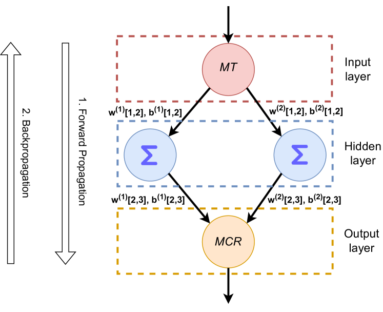
Figure 1. MLP neural network architecture.

Gradient boosting regression

estimates and constructs an additive model in a forward stage-wise manner. GBR (natekin2013gradient, ) can ensemble multiple prediction models (e.g., regression trees) to create a more accurate model (zhong2022machine, ).

$$\mathtt{MCR}^{\prime}_{\mathcal{P}{}i}=F_{\mathcal{E}}(\mathtt{MT}_{i,j})=\sum_{e=1}^{\mathcal{E}}h_{e}(\mathtt{MT}_{i,j}),$$

where the $h_{e}$ is a boosting estimator and $\mathcal{E}$ is a constant corresponding to the number of estimators (ensemble.methods, ) used by the fixed-size decision tree regressors.

5. Architecture Design

We present in this section the architecture design of our method implemented in the $DataCloud$ toolbox (nikolov2023container, ).

5.1. $DataCloud$

We designed the architecture of our method in the context of the $DataCloud$ (roman2022big, ) project supporting the lifecycle of microservices-based applications processing streams and batches of data on the computing continuum through the interaction of four tools.

$DEF-PIPE$

defines the application services and structure from the user input using a domain-specific language model to define the microservice requirements (tahmasebi2022dataclouddsl, );

$SIM-PIPE$

simulates the dataflow execution based on the microservice’s processing speed and memory size requirements before large-scale deployment (thomas2022sim, );

$ADA-PIPE$

receives the microservices, explores their requirements, such as processing and memory size, predicts the number of replicas for each microservice based on its resource requirements, adapts the execution, and sends to $DEP-PIPE$ for the deployment;

$DEP-PIPE$

deploys the dataflow processing microservices on the computing resources based on $ADA-PIPE$ schedules and manages their execution on multiple Kubernetes clusters at the user’s location or in the Cloud (simonet2022toward, ).

5.2. $ADA-PIPE$

Figure 2 illustrates the $ADA-PIPE$’s component with its replica prediction, consisting of seven components.

Microservice requirement analysis

receives resource needs $\mathtt{req}\left(m_{i}\right)$ of the user application microservices to update the trace. Moreover, it includes the simulation information of the microservice times provided by $SIM-PIPE$ to predict the microservices to the trace;

Microservice trace

consists of rows with the timestamp, microservice name, microservice container instance identifier, and the collected metrics (i.e., $\mathtt{MCR}_{\mathcal{P}{}i}$, $\mathtt{MT}_{i,j}$) (luo2021characterizing, );

Feature set

receives the dataset and extracts the microservice call rate $\mathtt{MCR}_{\mathcal{P}{}i}$ for a corresponding microservice time $\mathtt{MT}_{i,j}$. The ML models learn to fit the $\mathtt{MT}$ as the input to the $\mathtt{MCR}_{\mathcal{P}{}i}$ as the output;

ML hyperparameter design

component receives the feature set consisting of $\mathtt{MCR}_{\mathcal{P}{}i}$ and $\mathtt{MT}_{i,j}$ for fine-tuning and optimizing the ML models. It utilizes an exhaustive search to configure and tune the hyperparameters;

Prediction model

forecasts the microservice call rate based on the microservice time by utilizing the ML prediction models, including LR, MLP, and GBR (see Section 4);

Replica

component estimates the required instances to scale out from each microservice based on the multiplication between its predicted call rate $\mathtt{MCR}{{}^{\prime}}_{\mathcal{P}{}i}$ and time $\mathtt{MT}_{i,j}$;

Orchestration

manages the microservices on the Cloud virtual machines by utilizing the Kubernetes replica scaling based on the predicted microservice call rates and decisions taken by the integrated scheduler (mehran2022matching, ).

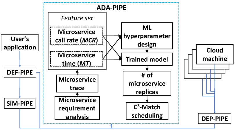
Figure 2. $ADA-PIPE$ architecture.

6. Experimental Design

This section presents our experimental design for the dataset preparation, testbed, and tuning of hyperparameters.

6.1. Dataset preparation

We validated our method using simulation based on an Alibaba microservice dataset available in a public repository. The dataset contains dataflows with various communication paradigms among over $1300$ microservices running on more than $90\,000$ containers for twelve hours, recorded in a time interval of $30\text{\,}\mathrm{s}\text{/}$ (luo2021characterizing, ). We selected $180\,000$ rows of the dataset, denoting the microservice times $\mathtt{MT}_{i,j}$= $0.01\text{\,}\mathrm{m}\mathrm{s}\mathrm{/}\mathrm{c}\mathrm{a}\mathrm{l}\mathrm{l}5859\text{\,}\mathrm{m}\mathrm{s}\mathrm{/}\mathrm{c}\mathrm{a}\mathrm{l}\mathrm{l}$, and the microservice call rates $\mathtt{MCR}_{\mathcal{P}{}i}$ = $0.025\text{\,}\mathrm{c}\mathrm{a}\mathrm{l}\mathrm{l}\mathrm{s}\mathrm{/}\mathrm{s}4874\text{\,}\mathrm{c}\mathrm{a}\mathrm{l}\mathrm{l}\mathrm{s}\mathrm{/}\mathrm{s}$.

6.2. Testbed design

We implemented ML algorithms in Python 3.9 using scikit-learn API (scikitlearn_api, ). Afterward, we compared the runtime performance of the algorithms on two machines:

• Google CoLaboratory (CoLab) with NVIDIA^® Tesla^(TM) T4 GPU accelerator and $16\text{\,}\mathrm{GB}\text{/}$ of memory;

• Personal device with an $8$-core Intel^® Core^(TM) i7-7600U processor and $16\text{\,}\mathrm{GB}\text{/}$ of memory.

6.3. ML hyperparameter design

This section presents the learning procedure of fine-tuning and optimization of the hyperparameters of the GBR and MLP models, summarized in Table 2, based on three steps: exhaustive search, hyperparameter tuning, and hyperparameter configuration. However, we rely on the default settings of ordinary least squares optimization for the LR model (scikit-lr, ).

6.3.1. Gradient boosting regressor

uses a learning curve to evaluate the changes in the training loss for different iterations based on the number of evaluators and the learning rate (see Figure 3(a)).

Exhaustive search

uses the GridSearchCV library of the ML toolkit scikit-learn and sets the number of estimators to $300$ and learning rate to $0.02$, which results in overfitting the training data.

Hyperparameter tuning

modifies the number of estimators in the range of $10170$ and the learning rate in the range of $0.020.4$ to converge to a stability point with a faster training time.

Hyperparameter configuration

sets the number of estimators to $15$ and the learning to rate to $0.4$ with an improved training score without overfitting and reduced training time. Figure 3(a) shows that, during the training loop, the model tunes each gradient tree or estimator to the previous tree model’s error until it reaches the maximum number of estimators set.

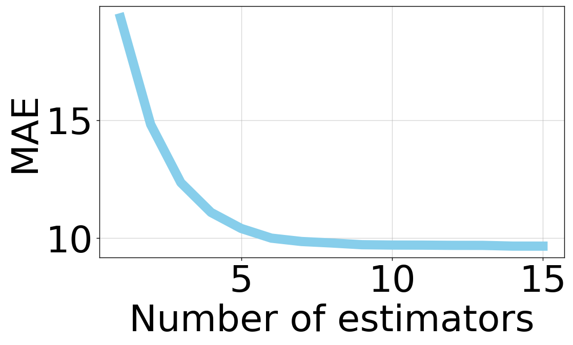
(a)

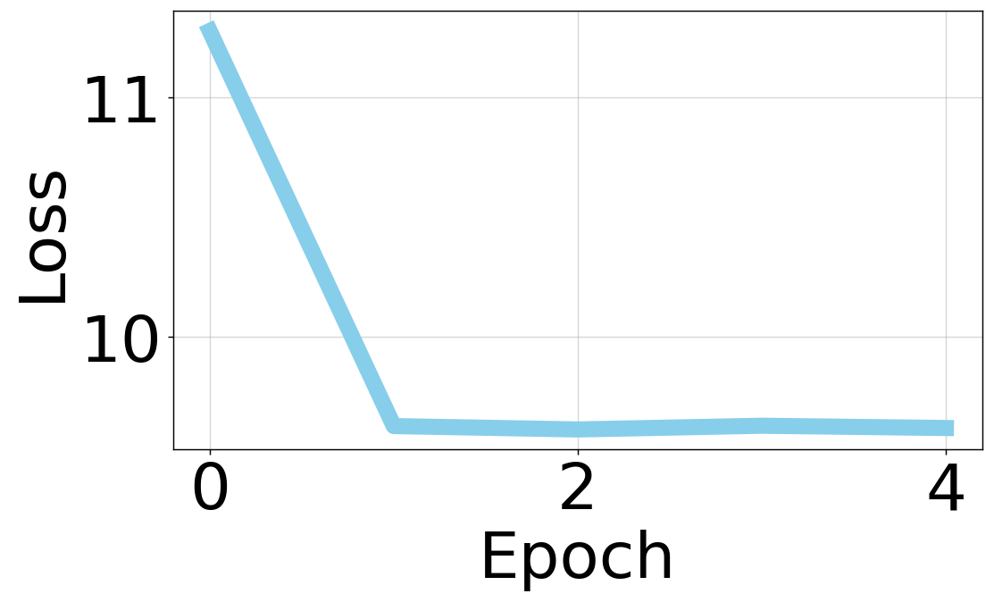
(b)

Figure 3. GBR and MLP losses.

6.3.2. Multilayer perceptron

uses the three-step learning curve evaluating the ML model’s performance through the changes in the training loss with different training iterations, number of layers, and number of neurons in the network (see Figure 3(b)).

Exhaustive search

uses the PyTorch library and sets the number of hidden layers to $3$, the number of neurons to $100$, and the learning rate to $0.4$ in $50$ epochs, overfitting the training data.

Hyperparameter tuning

decreases the learning rate to $0.0005$ to comprehend more about the training procedure. Afterward, we reduce the complexity of the model by lowering the number of neurons and hidden layers (see Figure 1) in each epoch because of the single input of $\mathtt{MT}_{i,j}$ in the dataset.

Hyperparameter configuration

of the MLP model with two epochs, one hidden layer of two neurons, and a learning rate of $0.003$ predicts the $\mathtt{MCR}_{\mathcal{P}{}i}$ without overfitting, as shown in Figure 3(b).

Table 2. ML hyperparameter design.

Model	Hyperparameter	Description	Value
MLP	Hidden layers	Number of hidden layers	1
	Optimizer	Optimization algorithm	Adam
	Learning rate	Learning step size at each iteration	$0.003$
	Loss	Error quantification between $\mathtt{MCR}^{\prime}_{\mathcal{P}{}i}$ and $\mathtt{MCR}_{\mathcal{P}{}i}$	L1Loss
GBR	Subsample	Ratio of training sample	0.8
	Learning rate	Coefficient shrinkage	$0.4$
	Number of estimators	Max. number of gradient trees for model boosting	$15$
	Max. depth	Maximum depth of a tree	$8$
	Min. samples split	Minimum number of samples for splitting the tree	$200$
	Min. samples leaf	Minimum number of samples for tree’s leaves	$40$
	Loss	MAE between $\mathtt{MCR}^{\prime}_{\mathcal{P}{}i}$ and $\mathtt{MCR}_{\mathcal{P}{}i}$	MAE

6.4. Evaluation metrics

In this section, we evaluate the performance of LR, MLP, and GBR prediction models using five metrics.

Pearson correlation coefficient

between the microservice time and its call rate in the Alibaba trace:

$$\frac{\sum\limits_{\mathcal{P}\in\mathcal{M}_{\mathcal{P}}\land m_{i}\in\mathcal{M}}\left(\mathtt{MT}_{i,j}-\overline{\mathtt{MT}_{i,j}}\right)\cdot\left(\mathtt{MCR}_{\mathcal{P}{}i}-\overline{\mathtt{MCR}_{\mathcal{P}{}i}}\right)}{\sqrt{\sum\limits_{\mathcal{P}\in\mathcal{M}_{\mathcal{P}}\land m_{i}\in\mathcal{M}}\left(\mathtt{MT}_{i,j}-\overline{\mathtt{MT}_{i,j}}\right)}\cdot\sqrt{\sum\limits_{\mathcal{P}\in\mathcal{M}_{\mathcal{P}}\land m_{i}\in\mathcal{M}}\left(\mathtt{MCR}_{\mathcal{P}{}i}-\overline{\mathtt{MCR}_{\mathcal{P}{}i}}\right)}}$$

where $\overline{\mathtt{MT}_{i,j}}$ and $\overline{\mathtt{MCR}_{\mathcal{P}{}i}}$ show the average microservice time and the call rate, respectively.

Predicted microservice call rate

$\mathtt{MCR}{{}^{\prime}}_{\mathcal{P}{}i}$ defined in Section 4.

Number of replicas

$\mathcal{L}_{i}$ defined in Section 3.

Mean absolute error

also referred to as L1Loss (L1Loss, ), represents the average sum of absolute differences between the predicted microservice call rates $\mathtt{MCR}^{\prime}_{\mathcal{P}{}i}$ and $\mathtt{MCR}_{\mathcal{P}{}i}$, respectively, in the testing and training:

$$\mathrm{MAE}={\frac{1}{\mathcal{N}_{\mathcal{M}}}}\cdot\sum\limits_{\mathcal{P}\in\mathcal{M}_{\mathcal{P}}\land m_{i}\in\mathcal{M}}\left|\mathtt{MCR}_{\mathcal{P}{}i}-\mathtt{MCR}^{\prime}_{\mathcal{P}{}i}\right|.$$

Mean absolute percentage error

($\mathrm{MAPE}$) quantifies the prediction accuracy of an ML model:

$$\mathrm{MAPE}={\frac{1}{\mathcal{N}_{\mathcal{M}}}\cdot\sum\limits_{\mathcal{P}\in\mathcal{M}_{\mathcal{P}}\land m_{i}\in\mathcal{M}}\left|\frac{\mathtt{MCR}_{\mathcal{P}{}i}-\mathtt{MCR}^{\prime}_{\mathcal{P}{}i}}{\mathtt{MCR}_{\mathcal{P}{}i}}\right|}.$$

7. Experimental Results

This section presents the performance evaluations of the ML models in predicting the microservice call rates and replicas.

7.1. Feature distribution and correlation

Figure 4 shows the distribution, correlation, and relative variation of the two features $\mathtt{MT}_{i,j}$ and $\mathtt{MCR}_{\mathcal{P}{}i}$ in the Alibaba dataset using the Pearson coefficient. The results denote that we achieve a high correlation $75\text{\,}\mathrm{\char 37\relax}\text{/}$ between both feature sets, denoting that the prediction is applied to a correlated set of features.

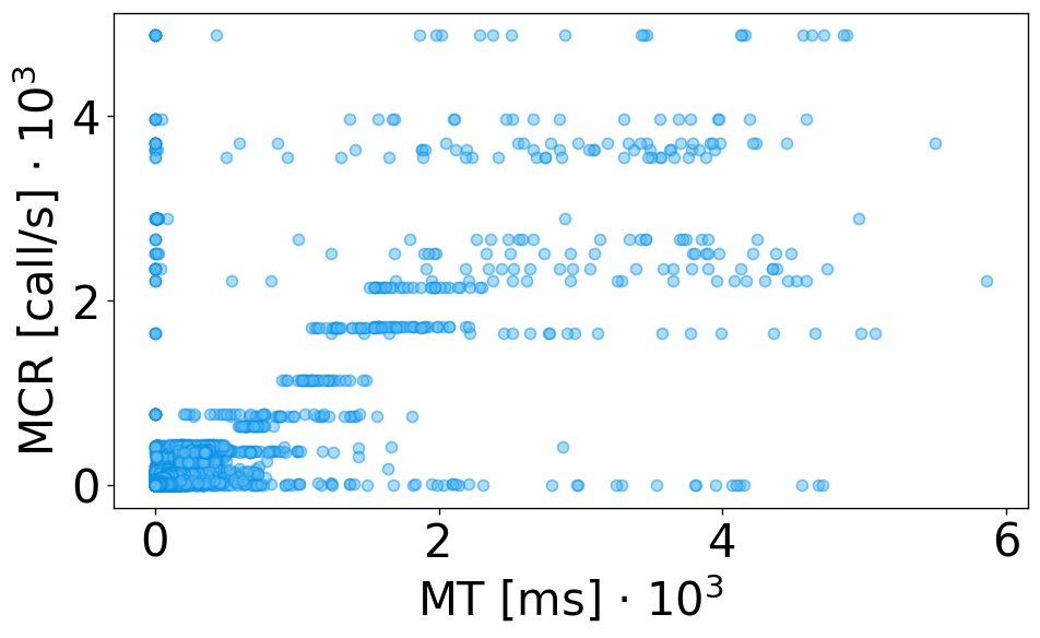
Figure 4. Distribution and correlation of $\mathtt{MT}_{i,j}$ and $\mathtt{MCR}_{\mathcal{P}{}i}$ in Alibaba microservices dataset.

7.2. Model fitting

Figure 5(a) shows that the LR model fits a linear relation between the predicted microservice call rate $\mathtt{MCR}^{\prime}_{\mathcal{P}{}i}$ and microservice time $\mathtt{MT}_{i,j}$. Figure 5(b) depicts fitting a linear MLP model to the test dataset. Although the model learns to fit a linear relation between the microservice time and call rate, it has a slightly lower MAE than the LR, as shown in Table 3. This indicates that the MLP model remains a proper fit for this dataset despite its neural network baseline imposing a computationally intensive method compared to LR and GBR. Figure 5(c) shows that the GBR ensemble model does not follow a linear pattern because it iteratively fits new decision tree regressors to the loss of the previous ensemble. In other words, the model continuously tunes and boosts its predictions by fitting a new subset of training data to the ensemble of previous models to create a single low-error predictive model.

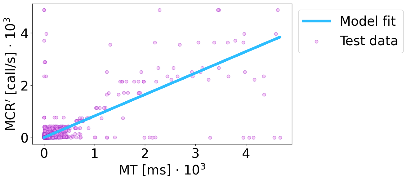
(a)

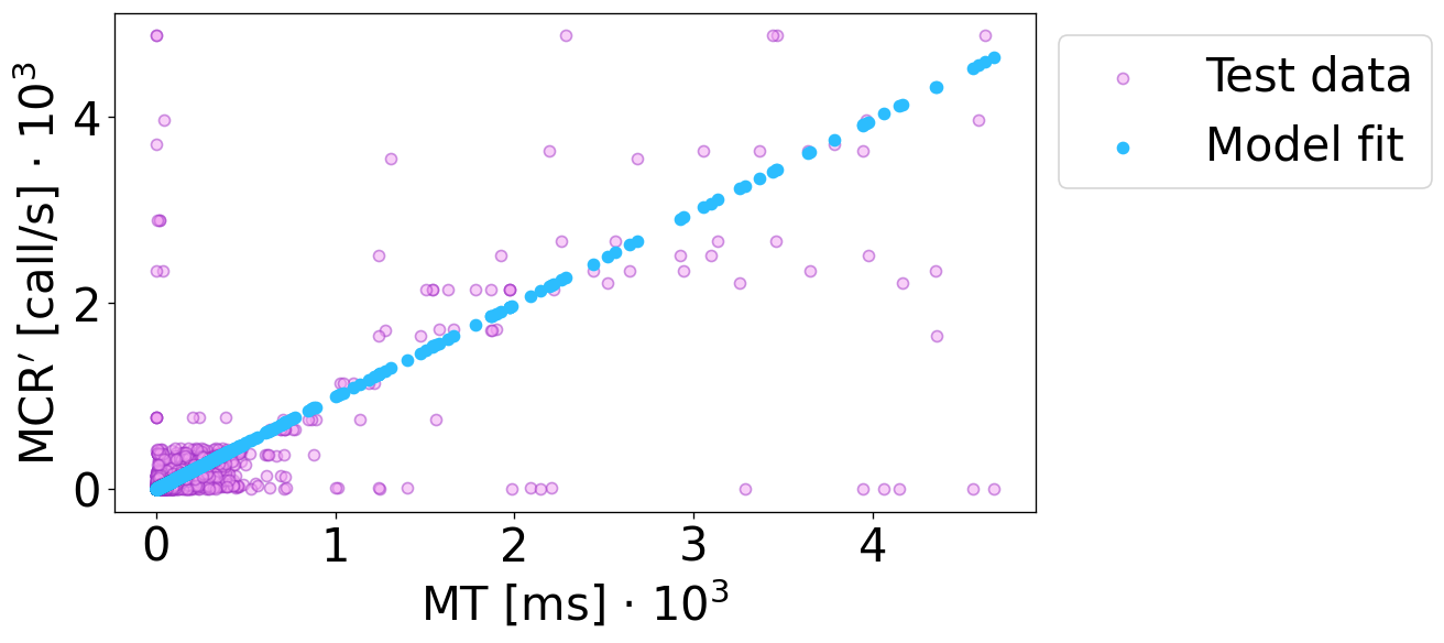
(b)

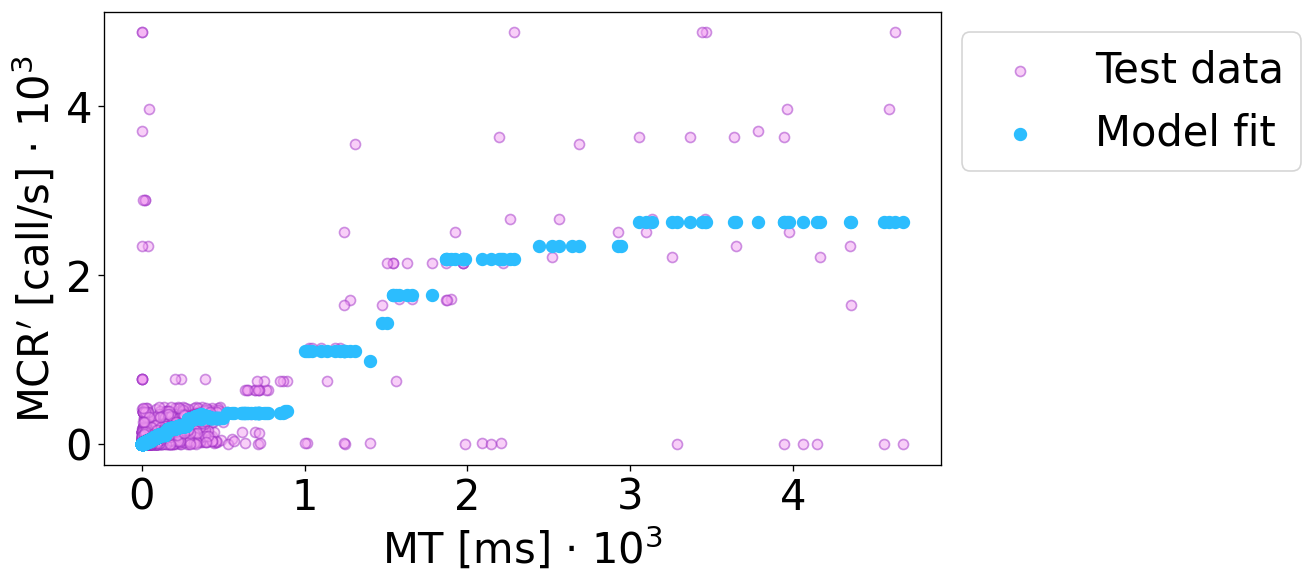
(c)

Figure 5. ML model fitting to the test dataset.

Table 3. MAE, MAPE, and training times of the prediction models.

Prediction model	MAE	MAPE	Training time [$\mathrm{s}\text{/}$]
LR	$10.2512.84$	$16.316.4$	$1.32$
MLP	$9.3\text{\,}\text{/}9.4\text{\,}\text{/}$	$16.516.7$	$1114$
GBR	$8.908.94$	$11.511.7$	$34.5$

7.3. Training time

Table 3 illustrates the superiority of the LR method that lowers the training time with the expense of increasing the prediction errors compared with the MLP and GBR. The neural network-based MLP increases the training time of the prediction, although it is based upon the linear models as defined in Section 4. However, the GBR model reaches a balance between the prediction errors, including the MAE and MAPE, and the training time of the training model.

7.4. Number of replicas

Table 4 shows that the ML models estimate the number of replicas by following almost close prediction errors. The results show that the GBR model reaches lower MAPE regarding replication prediction compared to the LR and MLP.

Table 4. MAPE of the prediction models.

Prediction model	MAPE
LR	$14.314.5$
MLP	$15.916.2$
GBR	$10.911.1$

8. Conclusion and Future Work

We explored and compared three ML methods to improve the resource provisioning affected by stochastic changes due to the users’ requirements by investigating the performance evaluation of a set of ML models on the monitoring data. We used three different ML models, LR, GBR, and MLP, that predict the microservice call rate based on the microservice time scheduled in the Alibaba Cloud resources. Since utilizing the MLP for this problem with one input and one output was complex, we set a small number of neurons and layers in its prediction model. The experimental results show that the GBR reduces the MAE and the MAPE compared to LR and MLP models. Moreover, the results show that the gradient boosting model estimates the number of replicas for each microservice close to the actual data without any prediction. In the future, we plan to explore integrating the ML models in the Kubernetes autoscaling component (horn2022multi, ) and evaluate the optimal deployment of microservices.

References

- (1) Christina Terese Joseph and K Chandrasekaran. Intma: Dynamic interaction-aware resource allocation for containerized microservices in cloud environments. Journal of Systems Architecture, 111:101785, 2020.
- (2) Narges Mehran, Zahra Najafabadi Samani, Dragi Kimovski, and Radu Prodan. Matching-based scheduling of asynchronous data processing workflows on the computing continuum. In 2022 IEEE International Conference on Cluster Computing (CLUSTER), pages 58–70, 2022.
- (3) Shutian Luo, Huanle Xu, Chengzhi Lu, Kejiang Ye, Guoyao Xu, Liping Zhang, Yu Ding, Jian He, and Chengzhong Xu. Characterizing microservice dependency and performance: Alibaba trace analysis. In Proceedings of the ACM Symposium on Cloud Computing, pages 412–426, 2021.
- (4) Hamidreza Arkian, Guillaume Pierre, Johan Tordsson, and Erik Elmroth. Model-based stream processing auto-scaling in geo-distributed environments. In ICCCN 2021-30th International Conference on Computer Communications and Networks, 2021.
- (5) Krzysztof Rzadca, Pawel Findeisen, Jacek Swiderski, Przemyslaw Zych, Przemyslaw Broniek, Jarek Kusmierek, Pawel Nowak, Beata Strack, Piotr Witusowski, Steven Hand, et al. Autopilot: workload autoscaling at google. In Proceedings of the Fifteenth European Conference on Computer Systems, pages 1–16, 2020.
- (6) Angelina Horn, Hamid Mohammadi Fard, and Felix Wolf. Multi-objective hybrid autoscaling of microservices in kubernetes clusters. In Euro-Par 2022: Parallel Processing: 28th International Conference on Parallel and Distributed Computing, pages 233–250. Springer, 2022.
- (7) Nikolay Nikolov, Yared Dejene Dessalk, Akif Quddus Khan, Ahmet Soylu, Mihhail Matskin, Amir H Payberah, and Dumitru Roman. Conceptualization and scalable execution of big data workflows using domain-specific languages and software containers. Internet of Things, page 100440, 2021.
- (8) Yury Gorishniy, Ivan Rubachev, Valentin Khrulkov, and Artem Babenko. Revisiting deep learning models for tabular data, 2023.
- (9) Yury Gorishniy, Ivan Rubachev, and Artem Babenko. On embeddings for numerical features in tabular deep learning, 2023.
- (10) Tianqi Chen, Tong He, Michael Benesty, Vadim Khotilovich, Yuan Tang, Hyunsu Cho, Kailong Chen, Rory Mitchell, Ignacio Cano, Tianyi Zhou, et al. Xgboost: extreme gradient boosting. R package version 0.4-2, 1(4):1–4, 2015.
- (11) Léo Grinsztajn, Edouard Oyallon, and Gaël Varoquaux. Why do tree-based models still outperform deep learning on typical tabular data? Advances in Neural Information Processing Systems, 35:507–520, 2022.
- (12) Shutian Luo, Huanle Xu, Chengzhi Lu, Kejiang Ye, Guoyao Xu, Liping Zhang, Jian He, and Chengzhong Xu. An in-depth study of microservice call graph and runtime performance. IEEE Transactions on Parallel and Distributed Systems, 33(12):3901–3914, 2022.
- (13) Shutian Luo, Huanle Xu, Kejiang Ye, Guoyao Xu, Liping Zhang, Guodong Yang, and Chengzhong Xu. The power of prediction: microservice auto scaling via workload learning. In Proceedings of the 13th Symposium on Cloud Computing, pages 355–369, 2022.
- (14) Joy Rahman and Palden Lama. Predicting the end-to-end tail latency of containerized microservices in the cloud. In 2019 IEEE International Conference on Cloud Engineering (IC2E), pages 200–210, 2019.
- (15) Yi-Lin Cheng, Ching-Chi Lin, Pangfeng Liu, and Jan-Jan Wu. High resource utilization auto-scaling algorithms for heterogeneous container configurations. In 23rd IEEE International Conference on Parallel and Distributed Systems (ICPADS), pages 143–150, 2017.
- (16) Fabiana Rossi, Valeria Cardellini, Francesco Lo Presti, and Matteo Nardelli. Geo-distributed efficient deployment of containers with kubernetes. Computer Communications, 159:161–174, 2020.
- (17) Sebastian Ştefan and Virginia Niculescu. Microservice-oriented workload prediction using deep learning. e-Informatica Software Engineering Journal, 16(1):220107, March 2022. Available online: 25 Mar. 2022.
- (18) Hangtao He, Linyu Su, and Kejiang Ye. Graphgru: A graph neural network model for resource prediction in microservice cluster. In 2022 IEEE 28th International Conference on Parallel and Distributed Systems (ICPADS), pages 499–506, 2023.
- (19) Zahra Najafabadi Samani, Narges Mehran, Dragi Kimovski, Shajulin Benedikt, Nishant Saurabh, and Radu Prodan. Incremental multilayer resource partitioning for application placement in dynamic fog. IEEE Transactions on Parallel and Distributed Systems, pages 1–18, 2023.
- (20) scikit-learn developers. Linear regression pipeline by scikit-learn. https://scikit-learn.org/stable/modules/linear_model.html#ordinary-least-squares, 2023.
- (21) The MathWorks, Inc. What Is a Linear Regression Model? https://www.mathworks.com/help/stats/what-is-linear-regression.html, 2023.
- (22) Kanad Keeni, Kenji Nakayama, and Hiroshi Shimodaira. Estimation of initial weights and hidden units for fast learning of multilayer neural networks for pattern classification. In IJCNN’99. International Joint Conference on Neural Networks. Proceedings (Cat. No. 99CH36339), volume 3, pages 1652–1656. IEEE, 1999.
- (23) PyTorch Contributors. Linear – pytorch 2.0 documentation. https://pytorch.org/docs/stable/generated/torch.nn.Linear.html#linear, 2023.
- (24) Alexey Natekin and Alois Knoll. Gradient boosting machines, a tutorial. Frontiers in neurorobotics, 7:21, 2013.
- (25) Zhiheng Zhong, Minxian Xu, Maria Alejandra Rodriguez, Chengzhong Xu, and Rajkumar Buyya. Machine learning-based orchestration of containers: A taxonomy and future directions. ACM Computing Surveys (CSUR), 54(10s):1–35, 2022.
- (26) scikit-learn developers. 1.11. ensemble methods – scikit-learn 1.3.0 documentation. https://scikit-learn.org/stable/modules/ensemble.html#gradient-boosting, 2023.
- (27) Nikolay Nikolov, Arnor Solberg, Radu Prodan, Ahmet Soylu, Mihhail Matskin, and Dumitru Roman. Container-based data pipelines on the computing continuum for remote patient monitoring. Computer, 56(10):40–48, 2023.
- (28) Dumitru Roman, Radu Prodan, Nikolay Nikolov, Ahmet Soylu, Mihhail Matskin, Andrea Marrella, Dragi Kimovski, Brian Elvesæter, Anthony Simonet-Boulogne, Giannis Ledakis, Hui Song, Francesco Leotta, and Evgeny Kharlamov. Big data pipelines on the computing continuum: Tapping the dark data. Computer, 55(11):74–84, 2022.
- (29) Shirin Tahmasebi, Amirhossein Layegh, Nikolay Nikolov, Amir H Payberah, Khoa Dinh, Vlado Mitrovic, Dumitru Roman, and Mihhail Matskin. Dataclouddsl: Textual and visual presentation of big data pipelines. In 2022 IEEE 46th Annual Computers, Software, and Applications Conference (COMPSAC), pages 1165–1171. IEEE, 2022.
- (30) Aleena Thomas, Nikolay Nikolov, Antoine Pultier, Dumitru Roman, Brian Elvesæter, and Ahmet Soylu. Sim-pipe dryrunner: An approach for testing container-based big data pipelines and generating simulation data. In 2022 IEEE 46th Annual Computers, Software, and Applications Conference (COMPSAC), pages 1159–1164. IEEE, 2022.
- (31) Anthony Simonet-Boulogne, Arnor Solberg, Amir Sinaeepourfard, Dumitru Roman, Fernando Perales, Giannis Ledakis, Ioannis Plakas, and Souvik Sengupta. Toward blockchain-based fog and edge computing for privacy-preserving smart cities. Frontiers in Sustainable Cities, page 136, 2022.
- (32) Lars Buitinck, Gilles Louppe, Mathieu Blondel, Fabian Pedregosa, Andreas Mueller, Olivier Grisel, Vlad Niculae, Peter Prettenhofer, Alexandre Gramfort, Jaques Grobler, Robert Layton, Jake VanderPlas, Arnaud Joly, Brian Holt, and Gaël Varoquaux. API design for machine learning software: experiences from the scikit-learn project. In ECML PKDD Workshop: Languages for Data Mining and Machine Learning, pages 108–122, 2013.
- (33) PyTorch Contributors. L1loss – pytorch 2.0 documentation. https://pytorch.org/docs/stable/generated/torch.nn.L1Loss.html#torch.nn.L1Loss, 2023.