Unruh-De Witt detectors, Bell-CHSH inequality and Tomita-Takesaki theory

Abstract

The interaction between Unruh-De Witt spin $1/2$ detectors and a real scalar field is scrutinized by making use of the Tomita-Takesaki modular theory as applied to the Von Neumann algebra of the Weyl operators. The use of the modular theory enables to evaluate in an exact way the trace over the quantum field degrees of freedom. The resulting density matrix is employed to the study of the Bell-CHSH correlator. It turns out that, as a consequence of the interaction with the quantum field, the violation of the Bell-CHSH inequality exhibits a decreasing as compared to the case in which the scalar field is absent.

I Introduction

The so-called Unruh-De Witt detectors serve as highly useful models that are largely employed in the study of relativistic quantum information, see [1, 2, 3] and refs. therein.

In the current work, we shall utilize spin $1/2$ Unruh-De Witt detectors to investigate the potential impact of a quantum relativistic scalar field on the Bell-CHSH inequality [4, 5]. More precisely, we shall start by considering the interaction of a pair of q-bits with a real Klein-Gordon field in Minkowski spacetime. The initial state of the Klein-Gordon field is identified as the vacuum state $|0\rangle$. Concerning the q-bits, the corresponding state will be taken as

$$|\psi\rangle_{AB}=\frac{|g_{A}\rangle\otimes|g_{B}\rangle+r|e_{A}\rangle\otimes|e_{B}\rangle}{\sqrt{1+r^{2}}},\;\;\;r\in[0,\,1]\;,$$ (1)

where, using the same notation of [2, 3], $|g_{j}\rangle$, $|e_{j}\rangle$, $j=A,B$ stand for the ground and excited states of the two-level Hamiltonian

$$h_{j}=\frac{1}{2}\Omega_{j}(\sigma_{j}^{z}+\mathbb{1}),\;\;\;\;j=A,\,B,$$ (2)

with $\sigma_{j}^{z}$ being the diagonal Pauli matrix along the $z$-direction. The states $|g_{j}\rangle$, $|e_{j}\rangle$ possess energy $0$ and $\Omega_{j}$, respectively. As it is customary in the study of entanglement, the indices $A,B$ refer to Alice and Bob which, according to the relativistic causality requirement, are located in the right and left Rindler wedges, Moreover, the parameter $r$ in expression (1) will enable us to interpolate between a product state, corresponding to $r=0$, and a maximally entangled state, i.e. when $r=1$.

For the Hamiltonian describing the interaction between the q-bits and the real scalar field $\varphi(x)$, we have [2, 3],

$$h_{Ij}(x)=f_{j}(x)\mu_{j}(\tau_{j}(x))\otimes\varphi(x),$$ (3)

where

$$\mu_{j}(\tau_{j})=\sigma_{j}^{+}e^{i\Omega_{j}\tau{j}}+\sigma_{j}^{-}e^{-i\Omega_{j}\tau{j}}$$ (4)

is the monopole moment of the detector $j$ with proper time $\tau_{j}$ [2, 3]. The matrices $\sigma^{\pm}$ stand for the ladder operators

$$\sigma_{j}^{+}|g_{j}\rangle =|e_{j}\rangle$$

$$\sigma_{j}^{-}|e_{j}\rangle =|g_{j}\rangle.$$

The functions $f_{j}(x)$ are smooth test functions with compact support, $f_{j}(x)\in{\cal C}_{0}^{\infty}(\mathbb{R}^{4})$.

At this stage, we need to specify the starting density matrix, namely

$$\rho_{AB\varphi}(0)=\rho_{AB}(0)\otimes|0\rangle\langle 0|\;,$$ (5)

where

$$\rho_{AB}(0)=|\psi\rangle_{AB}\;{}_{AB}\langle\psi|\;.$$ (6)

Furthermore, the time evolution of the initial density matrix, Eq.(5), is governed by the unitary operator

$$\mathcal{U}=Te^{-i\int d^{4}x(h_{IA}(x)+h_{IB}(x))},$$ (7)

where $T$ is the time ordering operator, i.e.

$$\rho_{AB\varphi}(t)=\mathcal{U}\;\rho_{AB\varphi}(0)\;\mathcal{U}^{\dagger}\;.$$ (8)

The next step is that of obtaining the density matrix ${\hat{\rho}}_{AB}$ for the q-bits system by tracing out the field modes:

$${\hat{\rho}}_{AB}={\rm Tr}_{\varphi}(\rho_{AB\varphi}(t))\;.$$ (9)

Finally, one is ready to evaluate the Bell-CHSH correlator

$$\langle\mathcal{C}\rangle = {\rm Tr}({\hat{\rho}}_{AB}\mathcal{C})$$

$$\mathcal{C} = (A+A^{\prime})B+(A-A^{\prime})B^{\prime}\;,$$ (10)

where $(A,A^{\prime})$, $(B,B^{\prime})$ are the Bell operators, see Section (IV). In that way we are able to investigate the violation of the Bell-CHSH inequality by taking into account the effects arising from the presence of the quantum field $\varphi(x)$, encoded in the density matrix ${\hat{\rho}}_{AB}$.

Having outlined the working setup, we proceed by stating our main result as well as by presenting the organization of the present work:

• the first aspect which we would like to highlight is the role which will be played by the unitary Weyl operators

  $$W_{f_{j}}=e^{i{\varphi}(f_{j})}\;,\qquad j=A,B\;,$$ (11)

  where $\varphi(f_{j})$ is the smeared field [6]

  $$\varphi(f_{j})=\int d^{4}x\;f_{j}(x)\varphi(x)\;.$$ (12)

  As one can figure out, these operators arise from the evolution operator $\mathcal{U}$, as discussed in Sect.(III). It is well established that the operators $W(f_{j})$ enjoy a rich algebraic structure, giving rise to a von Neumann algebra [6, 7, 8, 9, 10]. In particular, from the Reeh-Schlieder theorem [6, 7], it follows that the vacuum state $|0\rangle$ is both cyclic and separating for the aforementioned von Neumann algebra,

• These properties enable us to make use of the powerful Tomita-Takesaki modular theory [11]. As shown in [8, 9, 10], the modular theory is very well suited for the algebra of the Weyl operators. In particular, as it will be discussed in Section (III), the modular operators $(j,\delta)$ provide an exact evaluation of the correlation functions of the Weyl operators in terms of the inner products between Alice’s and Bob’s test functions $f_{A}$ and $f_{B}$.

• As a consequence, as detailed in Section (IV) and Section (V), the impact of the quantum field $\varphi$ on the violation of the Bell-CHSH inequality can be evaluated in closed form. Notably, it turns out that the violation of the Bell-CHSH inequality exhibits a decreasing behavior as compared to the case in which the field $\varphi$ is absent. This behavior is clearly visible through the exponential factors arising from the correlation functions of the Weyl operators, as exemplified in equation (65).

II Evaluation of the q-bits density matrix in the case of the $\delta$-coupled detectors

Let us begin the study of the denisty matrix ${\hat{\rho}}_{AB}$ by considering the so-called $\delta$-coupling [2, 3], corresponding to the regime in which the interaction between the q-bits and the scalar field $\varphi$ occurs at very short timescales, described thorugh $\delta$-functions of the proper times of the two detectors $(A,B)$. Following [2, 3], the evolution operator is given by $\mathcal{U}=\mathcal{U}_{A}\otimes\mathcal{U}_{B}$, where the unitary operator for the detector $j=A,B$ is

$$\mathcal{U}_{j}=e^{-i\mu_{j}(\tau_{j0})\otimes\varphi(f_{j})},$$ (13)

with the commutation relation

$$\left[\mathcal{U}_{A},\mathcal{U}_{B}\right]=0.$$ (14)

Using the algebra of the Pauli matrices, it is easy to show that expression (13) can be written as

$$\mathcal{U}_{j}=\mathbb{1}\otimes c_{j}-i\mu_{j}(\tau_{j0})\otimes s_{j},$$ (15)

where $c_{j}\equiv\cos\varphi(f_{j})$ and $s_{j}\equiv\sin\varphi(f_{j})$. Given the initial matrix density $\rho_{AB\varphi}(0)$, Eq.(5), its evolution reads

$$\rho_{AB\varphi} =\left(\mathcal{U}_{A}\otimes\mathcal{U}_{B}\right)\rho_{AB\varphi}(0)\;\mathcal{U}_{A}^{\dagger}\otimes\mathcal{U}_{B}^{\dagger}$$

$$=\left(\mathbb{1}_{A}\otimes\mathbb{1}_{B}c_{A}c_{B}\right.$$

$$\quad-i\mathbb{1}_{A}\otimes\mu_{B}c_{A}s_{A}$$

$$\quad-i\mu_{A}\otimes\mathbb{1}_{B}s_{A}c_{B}$$

$$\quad\left.-\mu_{A}\otimes\mu_{B}s_{A}s_{B}\right)\rho_{AB}(0)\otimes|0\rangle\langle 0|$$

$$\times\left(\mathbb{1}_{A}\otimes\mathbb{1}_{B}c_{A}c_{B}\right.$$

$$\quad+i\mathbb{1}_{A}\otimes\mu_{B}c_{A}s_{A}$$

$$\quad+i\mu_{A}\otimes\mathbb{1}_{B}s_{A}c_{B}$$

$$\quad\left.-\mu_{A}\otimes\mu_{B}s_{A}s_{B}\right)\;.$$ (16)

Taking the trace over $\varphi$, we get

$$\hat{\rho}_{AB}= \rho_{AB}(0)\langle c_{A}^{2}c_{B}^{2}\rangle-\rho_{AB}(0)(\mu_{A}\otimes\mu_{B})\langle c_{A}c_{B}s_{A}s_{B}\rangle$$

$$+(\mathbb{1}_{A}\otimes\mu_{B})\rho_{AB}(0)(\mathbb{1}_{A}\otimes\mu_{B})\langle c_{A}^{2}s_{B}^{2}\rangle$$

$$+(\mathbb{1}_{A}\otimes\mu_{B})\rho_{AB}(0)(\mu_{A}\otimes\mathbb{1}_{B})\langle c_{A}s_{A}c_{B}s_{B}\rangle$$

$$+(\mu_{A}\otimes\mathbb{1}_{B})\rho_{AB}(0)(\mu_{A}\otimes\mathbb{1}_{B})\langle c_{A}c_{B}s_{A}s_{B}\rangle$$

$$+(\mu_{A}\otimes\mathbb{1}_{B})\rho_{AB}(0)(\mu_{A}\otimes\mathbb{1}_{B})\langle s_{A}^{2}c_{B}^{2}\rangle$$

$$-(\mu_{A}\otimes\mu_{B})\rho_{AB}(0)\langle c_{A}s_{A}c_{B}s_{B}\rangle$$

$$+(\mu_{A}\otimes\mu_{B})\rho_{AB}(0)(\mu_{A}\otimes\mu_{B})\langle s_{A}^{2}s_{B}^{2}\rangle\;,$$ (17)

where $\langle c_{A}c_{B}s_{A}s_{B}\rangle$, etc., denotes the expectation value of the Weyl operators, namely

$$\langle c_{A}c_{B}s_{A}s_{B}\rangle=\langle 0|c_{A}c_{B}s_{A}s_{B}|0\rangle\;.$$ (18)

As we shall see in the next Section, these correlation functions will be handled in closed form by means of the Tomita-Takesaki theory. Once the density matrix ${\hat{\rho}}_{AB}$ is known, one can proceed with the investigation of the Bell-CHSH correlator, i.e.

$$\langle{\cal C}\rangle = {\rm Tr}({\hat{\rho}}_{AB}\;{\cal C})$$

$${\cal C} = (A-A^{\prime})B+(A-A^{\prime})B^{\prime}\;,$$ (19)

where $(A,A^{\prime})$ and $(B,B^{\prime})$ stand for Alice’s and Bob’s Bell’s operators:

$$A = A^{\dagger}\;,\quad A^{\prime}=A^{\prime\dagger}\;,\quad B=B^{\dagger}\;,\quad B^{\prime}=B^{\prime\dagger}$$

$$A^{2} = A^{\prime 2}=B^{2}=B^{\prime 2}=1$$

$$\left[A,B\right] = [A,B^{\prime}]=[A^{\prime},B]=[A^{\prime},B^{\prime}]=0\;.$$ (20)

The Bell-CHSH inequality is said to be violated whenever

$$2<|\langle{\cal C}\rangle|\leq 2\sqrt{2}\;,$$ (21)

where the maximum value $2\sqrt{2}$ is known as the Tsirelson bound [12]. The detailed analysis of Eq.(19) can be found in Section (IV).

III Tomita-Takesaki modular theory theory and the von Neumann algebra of the Weyl Operators

In order to face the evaluation of the correlation functions of the Weyl operators, Eq.(18), it is worth to provide a short account on some basic features of the properties of the related von Neumann algebra. Let us begin by reminding the expression of the causal Pauli-Jordan distribution $\Delta_{PJ}(x-y)$:

$$[\varphi(x),\varphi(y)] = i\Delta_{PJ}(x-y)$$

$$i\Delta_{PJ}(x-y)\! = \!\!\int\!\!\frac{d^{4}k}{(2\pi)^{3}}\varepsilon(k^{0})\delta(k^{2}-m^{2})e^{-ik(x-y)}\;,$$

with $\varepsilon(x)\equiv\theta(x)-\theta(-x)$, As it is well known, $\Delta_{PJ}(x-y)$ is Lorentz invariant and vanishes when $x$ and $y$ are space-like

$$\Delta_{PJ}(x-y)=0\;,\quad{\rm for}\quad(x-y)^{2}<0\;.$$ (23)

Let $\mathcal{O}$ be and open region of the Minkowski spacetime and let $\mathcal{M}(\mathcal{O})$ be the space of test functions $\in\mathcal{C}_{0}^{\infty}(\mathbb{R}^{4})$ with support contained in $\mathcal{O}$:

$$\mathcal{M}(\mathcal{O})=\{f\,|supp(f)\subseteq\mathcal{O}\}.$$ (24)

One introduces the symplectic complement [8, 9] of $\mathcal{M}(\mathcal{O})$ as

$$\mathcal{M^{\prime}}(\mathcal{O})=\{g\,|\Delta_{PJ}(g,f)=0,\;\forall f\in\mathcal{M}(\mathcal{O})\},$$ (25)

that is, $\mathcal{M}(\mathcal{O})$ is given by the set of all test functions for which the smeared Pauli-Jordan expression $\Delta_{PJ}(f,g)$ vanishes for any $f$ belonging to $\mathcal{M}(\mathcal{O})$

$$\left[\varphi(f),\varphi(g)\right]=i\Delta_{PJ}(f,g)\;.$$ (26)

The symplectic complement $\mathcal{M^{\prime}}(\mathcal{O})$ allows us to rephrase causality, Eq.(23), as [8, 9]

$$\left[\varphi(f),\varphi(g)\right]=0,$$ (27)

whenever $f\in\mathcal{M}(\mathcal{O})$ and $g\in\mathcal{M^{\prime}}(\mathcal{O})$.

We proceed by introducing the Weyl operators [8, 9, 10], a class of unitary operators obtained by exponentiating the smeared field

$$W_{h}=e^{i{\varphi}(h)}.$$ (28)

Using the Baker–Campbell–Hausdorff formula and the commutation relation (LABEL:PJ), it turns out that the Weyl operators give rise to the following algebraic structure:

$$W_{f}W_{g} =e^{-\frac{i}{2}\Delta_{\textrm{PJ}}(f,g)}\;W_{(f+g)},$$

$$W_{f}^{\dagger}W_{f} =W_{f}W_{f}^{\dagger}=1,$$

$$W^{\dagger}_{f} =W_{(-f)}.$$ (29)

Furthermore, for $f$ and $g$ space-like, the Weyl operators $W_{f}$ and $W_{g}$ commute. Expanding the field in terms of creation and annihilation operators, see [10], one can compute the expectation value of the Weyl operator, finding

$$\langle 0|W_{h}|0\rangle=\;e^{-\frac{1}{2}{\lVert h\rVert}^{2}},$$ (30)

where $||h||^{2}=\langle h|h\rangle$ and

$$\langle f|g\rangle = \int\frac{d^{3}k}{(2\pi)^{3}}\frac{1}{2\omega_{k}}f(\omega_{k},\vec{k})^{*}g(\omega_{k},\vec{k})$$

$$f(\omega_{k},\vec{k}) = \int d^{4}x\;e^{ikx}f(x)\;,$$ (31)

is the Lorentz invariant inner product between the test functions $(f,g)$ [8, 9, 10]. Taking now all possible products and linear combinations of the Weyl operators defined on $\mathcal{M}(\mathcal{O})$, gives rise to a von Neumann algebra $\mathcal{A}(\mathcal{M})$. In particular, from the the Reeh-Schlieder theorem [6, 7, 8, 9], it turns out that the vacuum state $|0\rangle$ is both cyclic and separating for the von Neumann algebra $\mathcal{A}$. Therefore, we can make use of the Tomita-Takesaki modular theory [11, 7, 8, 9, 10] and introduce the anti-linear unbounded operator $S$ whose action on the von Neumann algebra $\mathcal{A}(\mathcal{M})$ is defined as

$$S\;a|0\rangle=a^{\dagger}|0\rangle,\qquad\forall a\in\mathcal{A}(\mathcal{M}),$$ (32)

from which it follows that $S^{2}=1$ and $S|0\rangle=|0\rangle$. By performing a polar decomposition of the operator $S$ [11, 7, 8, 9, 10], one gets

$$S=J\Delta^{1/2},$$ (33)

where $J$ is anti-unitary and $\Delta$ is positive and self-adjoint. These modular operators satisfy the following properties [11, 7, 8, 9, 10]:

$$J\Delta^{1/2}J =\Delta^{-1/2},\quad\,\,\Delta^{\dagger}=\Delta,$$

$$S^{\dagger} =J\Delta^{-1/2},\,\,\,\,\,J^{\dagger}=J,$$

$$\Delta =S^{\dagger}S,\quad\,\,\,\,\,\,J^{2}=1.$$ (34)

According to the Tomita-Takesaki theorem [11, 7, 8, 9, 10], one has that $J\mathcal{A}(\mathcal{M})J=\mathcal{A}^{\prime}(\mathcal{M})$, that is, upon conjugation by the operator $J$, the algebra $\mathcal{A}(\mathcal{M})$ is mapped into its commutant $\mathcal{A^{\prime}}(\mathcal{M})$, namely:

$$\mathcal{A^{\prime}}(\mathcal{M})=\{\;a^{\prime}\,|\;[a,a^{\prime}]=0,\forall a\in\mathcal{A}(\mathcal{M})\;\}.$$ (35)

The Tomita-Takesaki modular theory is particularly suited for the analysis of the Bell-CHSH inequality within the framework of relativistic Quantum Field Theory [8, 9]. As shown in [10], it gives a way of constructing in a purely algebraic way Bob’s operators from Alice’s ones by making use of the modular conjugation $J$. That is, given Alice’s operator $A_{f}$, one can assign the operator $B_{f}=JA_{f}J$ to Bob, with the guarantee that they commute with each other since by the Tomita-Takesaki theorem the operator $B_{f}=JA_{f}J$ belongs to the commutant $\mathcal{A^{\prime}}(\mathcal{M})$ [10].

A very useful result on the Tomita-Takesaki modular theory, proven by [13, 14], enables one to lift the action of the modular operatos $(J,\Delta)$ to the space of the test functions. In fact, when equipped with the Lorentz-invariant inner product $\langle f|g\rangle$, Eq.(31), the set of test functions give rise to a complex Hilbert space $\mathcal{F}$ which enjoys several features. More precisely, it turns out that the subspaces $\mathcal{M}$ and $i\mathcal{M}$ are standard subspaces for $\mathcal{F}$ [13], meaning that: i) $\mathcal{M}\cap i\mathcal{M}=\{0\}$; ii) $\mathcal{M}+i\mathcal{M}$ is dense in $\mathcal{F}$. According to [13], for such subspaces it is possible to set a modular theory analogous to that of the Tomita-Takesaki. One introduces an operator $s$ acting on $\mathcal{M}+i\mathcal{M}$ as

$$s(f+ih)=f-ih.\;,$$ (36)

for $f,h\in\mathcal{M}$. Notice that with this definition, it follows that $s^{2}=1$. Using the polar decomposition, one has:

$$s=j\delta^{1/2},$$ (37)

where $j$ is an anti-unitary operator and $\delta$ is positive and self-adjoint. Similarly to the operators $(J,\,\Delta)$, the operators $(j,\,\delta)$ fulfill the following properties [13]:

$$j\delta^{1/2}j =\delta^{-1/2},\,\,\,\,\,\,\delta^{\dagger}=\delta$$

$$s^{\dagger} =j\delta^{-1/2},\,\,\,j^{\dagger}=j$$

$$\delta =s^{\dagger}s,\,\,\,\,\,\,\,\,\,\,\,j^{2}=1.$$ (38)

Moreover, as shown in [13], a test function $f$ belongs to $\mathcal{M}$ if and only if

$$sf=f\;.$$ (39)

In fact, suppose that $f\in\mathcal{M}$. On general grounds, owing to Eq.(36), one writes

$$sf=h_{1}+ih_{2}\;,$$ (40)

for some $(h_{1},h_{2})$. Since $s^{2}=1$ it follows that

$$f=s(h_{1}+ih_{2})=h_{1}-ih_{2}\;,$$ (41)

so that $h_{1}=f$ and $h_{2}=0$. In much the same way, one has that $f^{\prime}\in\mathcal{M}^{\prime}$ if and only if $s^{\dagger}f^{\prime}=f^{\prime}$.

The lifting of the action of the operators $(J,\Delta)$ to the space of test functions is thus achieved by [14]

$$Je^{i{\varphi}(f)}J=e^{-i{\varphi}(jf)},\quad\Delta e^{i{\varphi}(f)}\Delta^{-1}=e^{i{\varphi}(\delta f)}.$$ (42)

Also, it is worth noting that if $f\in\mathcal{M}\implies jf\in\mathcal{M}^{\prime}$. This property follows from

$$s^{\dagger}(jf)=j\delta^{-1/2}jf=\delta f=j(j\delta f)=j(sf)=jf\;.$$ (43)

It is also worth reminding that, in the case of wedge regions in Minkowski spacetime, the spectrum of $\delta$ coincides with the positive real line, i.e., $\log(\delta)=\mathbb{R}$ [15], being an unbounded operator with continuous spectrum.

We have now all ingredients for the evaluation of the correlation functions of the Weyl operators. Looking at expression (17), it is easy to realize that te basic quantity to be computed is of the kind

$$\langle e^{i\varphi(f_{A})}e^{\pm i\varphi(f_{B})}\rangle=\langle e^{i(\varphi(f_{A})\pm\varphi(f_{B}))}\rangle=e^{-\frac{1}{2}||f_{A}\pm f_{B}||^{2}}\;,$$ (44)

so that we need to evaluate the following norms $(||f_{A}||^{2},||f_{B}||^{2})$ and the inner product $\langle f_{A}|f_{B}\rangle$. We focus first on Alice’s test function $f_{A}$. We require that $f_{A}\in{\cal M(O)}$ where ${\cal O}$ is taken to be located in the right Rindler wedge. Following [8, 9, 10], the test function $f_{A}$ can be further specified by relying on the spectrum of the operator $\delta$. Ppicking up the spectral subspace specified by $[\lambda^{2}-\varepsilon,\lambda^{2}+\varepsilon]\subset(0,1)$ and introducing the normalized vector $\varphi$ belonging to this subspace, one writes

$$f_{A}=\eta(1+s)\varphi\;,$$ (45)

where $\eta$ is an arbitrary parameter. As required by the setup outlined above, equation (45) ensures that

$$sf_{A}=f_{A}\;.$$ (46)

We notice that $j\varphi$ is orthogonal to $\varphi$, i.e., $\langle\varphi|j\varphi\rangle=0$. In fact, from

$$\delta^{-1}(j\varphi)=j(j\delta^{-1}j)\varphi=j(\delta\varphi),$$ (47)

it follows that the modular conjugation $j$ exchanges the spectral subspace $[\lambda^{2}-\varepsilon,\lambda^{2}+\varepsilon]$ into $[1/\lambda^{2}-\varepsilon,1/\lambda^{2}+\varepsilon]$. Concerning now Bob’s test function $f_{B}$, we make use of the modular conjugation operator $j$ and define

$$f_{B}=jf_{A}\;,$$ (48)

so that

$$s^{\dagger}f_{B}=f_{B}$$ (49)

meaning that, as required by the relativistic causality, $f_{B}$ belongs to the symplectic complement $\mathcal{M^{\prime}}(\mathcal{O})$, located in the left Rindler wedge, namely: $f_{B}\in\mathcal{M^{\prime}}(\mathcal{O})$. Finally, taking into account that $\varphi$ belongs to the spectral subspace $[\lambda^{2}-\varepsilon,\lambda^{2}+\varepsilon]$, it follows that [10],

$$||f_{A}||^{2} =||jf_{A}||^{2}=\eta^{2}(1+\lambda^{2})$$

$$\langle f_{A}|jf_{A}\rangle =2\eta^{2}\lambda\;.$$ (50)

IV Analysis of the Bell-CHSH inequality

We are now ready to investigate the Bell-CHSH inequality, Eq.(19). Let us begin by defining the Bell operators [8, 9, 16]:

$$A|g_{A}\rangle = e^{i\alpha}|e_{A}\rangle\;,\qquad A|e_{A}\rangle=e^{-i\alpha}|g_{A}\rangle$$

$$A^{\prime}|g_{A}\rangle = e^{i\alpha^{\prime}}|e_{A}\rangle\;,\qquad A^{\prime}|e_{A}\rangle=e^{-i\alpha^{\prime}}|g_{A}\rangle$$

$$B|g_{B}\rangle = e^{-i\beta}|e_{B}\rangle\;,\qquad B|e_{B}\rangle=e^{i\beta}|g_{B}\rangle$$

$$B^{\prime}|g_{B}\rangle = e^{-i\beta^{\prime}}|e_{B}\rangle\;,\qquad B^{\prime}|e_{B}\rangle=e^{i\beta^{\prime}}|g_{B}\rangle\;,$$ (51)

which fulfill the whole set of conditions (20). The parameters $(\alpha,\alpha^{\prime},\beta,\beta^{\prime})$ are the four Bell’s angles entering the Bell-CHSH inequality, These parameters will be chosen at the best convenience.

Reminding that the initial state for $AB$ is

$$|\psi\rangle_{AB}=\frac{|g_{A}\rangle\otimes|g_{B}\rangle+r|e_{A}\rangle\otimes|e_{B}\rangle}{\sqrt{1+r^{2}}},\;\;\;r\in[0,\,1]\;,$$ (52)

and making use of

$$\mu_{A}|g_{A}\rangle=e^{i\Omega_{A}\tau_{A}^{0}}|e_{A}\rangle\;,\qquad\mu_{A}|e_{A}\rangle=e^{-i\Omega_{A}\tau_{A}^{0}}|g_{A}\rangle,$$ (53)

and similar expression for $\mu_{B}$, for the Bell-CHSH correlator $\langle C\rangle$ we get

$$\langle\mathcal{C}\rangle =\frac{2r}{1+r^{2}}[\cos(\alpha+\beta)\langle c_{A}^{2}c_{B}^{2}\rangle$$

$$\quad+\cos(\alpha-\beta+2\omega_{B})\langle c_{A}^{2}s_{B}^{2}\rangle$$

$$\quad+\cos(\alpha-\beta-2\omega_{A})\langle s_{A}^{2}c_{B}^{2}\rangle$$

$$\quad+\cos(\alpha+\beta-2\omega_{A}-2\omega_{B})\langle s_{A}^{2}s_{B}^{2}\rangle]$$

$$\left.\quad+2\cos(\alpha-\omega_{A}-\beta+\omega_{B})\langle c_{A}s_{A}c_{B}s_{B}\rangle\right.$$

$$\quad-2\cos(\alpha-\omega_{A}+\beta-\omega_{B})\langle c_{A}s_{A}c_{B}s_{B}\rangle$$

$$\quad+(\alpha\rightarrow\alpha^{\prime})+(\beta\rightarrow\beta^{\prime})$$

$$\quad-(\alpha\rightarrow\alpha^{\prime},\,\beta\rightarrow\beta^{\prime}),$$ (54)

where $\omega_{A}\equiv\Omega_{A}\tau_{A}^{0}$ and $\omega_{B}\equiv\Omega_{B}\tau_{B}^{0}$. Furthermore, by employing expressions (50), it follows that

$$\langle\mathcal{C}\rangle= \frac{2r}{1+r^{2}}\left\{\frac{1}{4}\cos(\alpha+\beta)\left[1+2e^{-2(1+\lambda^{2})\eta^{2}}\right.\right.$$

$$+\frac{1}{2}e^{-4(1+\lambda)^{2}\eta^{2}}+\frac{1}{2}e^{-4(1-\lambda)^{2}\eta^{2}}\left.\right]$$

$$+\frac{1}{4}\left(\cos(\alpha-\beta+2\omega_{B})+\cos(\alpha-\beta+2\omega_{A})\right)$$

$$\times\left[1-\frac{1}{2}e^{-4(1+\lambda)^{2}\eta^{2}}-\frac{1}{2}e^{-4(1-\lambda)^{2}\eta^{2}}\right]$$

$$+\frac{1}{4}\cos(\alpha+\beta-2\omega_{A}-2\omega_{B})$$

$$\times\left.\left[1-2e^{-2(1+\lambda^{2})\eta^{2}}+\frac{1}{2}e^{-4(1+\lambda)^{2}\eta^{2}}+\frac{1}{2}e^{-4(1-\lambda)^{2}\eta^{2}}\right]\right\}$$

$$+\left(\cos(\alpha-\beta-\omega_{A}+\omega_{B})-\cos(\alpha+\beta-\omega_{A}-\omega_{B})\right)$$

$$\times\frac{1}{4}\left[\frac{1}{2}e^{-4(1-\lambda)^{2}\eta^{2}}-\frac{1}{2}e^{-4(1+\lambda)^{2}\eta^{2}}\right]$$

$$+(\alpha\rightarrow\alpha^{\prime})+(\beta\rightarrow\beta^{\prime})-(\alpha\rightarrow\alpha^{\prime},\,\beta\rightarrow\beta^{\prime}).$$ (55)

From this expression one learns several things:

• the contribution arising from the scalar field $\varphi$ is encoded in the terms containing the exponentials $e^{-4\eta^{2}(1\pm\lambda)^{2}}$ and $e^{-2\eta^{2}(1+\lambda^{2})}$. It is worth reminding here that the parameter $\eta^{2}$ is related to the norm of the test function $f_{A}$, Eqs.(50).

• when the quantum field $\varphi$ is removed, i.e. $\eta^{2}\rightarrow 0$, expression (55) reduces to the usual Bell-CHSH inequality, namely

  $$\langle{\cal C}\rangle_{\eta=0} = \frac{2r}{1+r^{2}}\left(\cos(\alpha+\beta)+\cos(\alpha^{\prime}+\beta)\right)$$ (56)

  $$+ \frac{2r}{1+r^{2}}\left(\cos(\alpha+\beta^{\prime})-\cos(\alpha^{\prime}+\beta^{\prime})\right)\;.$$

  It is known that the angular part of Eq.(56) is maximized by [8, 9]:

  $$\alpha=0\;,\qquad\beta=-\frac{\pi}{4}\;\qquad\alpha^{\prime}=\frac{\pi}{2}\;,\qquad\beta^{\prime}=\frac{\pi}{4}\;,$$ (57)

  yielding

  $$\langle{\cal C}\rangle_{\eta=0}=2\sqrt{2}\frac{2r}{1+r^{2}}\;,$$ (58)

  which, for a maximally entangled state, $r=1$, gives Tsirelson’s bound

  $$\langle{\cal C}\rangle_{\eta=0,r=1}=2\sqrt{2}\;.$$ (59)

• however, when $\eta^{2}\neq 0$, i.e. when the quantum field $\varphi$ is present, the exponential factors $e^{-4\eta^{2}(1\pm\lambda)^{2}}$ and $e^{-2\eta^{2}(1+\lambda^{2})}$ have the effect of producing a damping, resulting in a decreasing of the violation of the Bell-CHSH inequality as compared to the pure Quantum Mechanical case, as it can be seen from Fig.(1) and Fig.(2), where the plot of the quantity

  $${\cal R}=\langle C\rangle-\langle C\rangle_{\eta=0}\;,$$ (60)

  is depicted. A damping behavior is signaled by ${\cal R}\leq 0$.

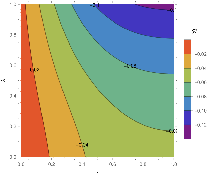
Figure 1: Contour plot exhibiting the negative behavior of $\cal R$ for as a function of $\lambda$ and $r$, for $\omega_{A}=0.5$, $\omega_{B}=0.6$, $\eta=0.1$. The four Bell’s angles $(\alpha,\alpha^{\prime},\beta,\beta^{\prime})$ are chosen as in Eq.(57).

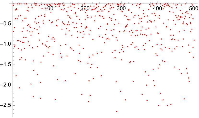
Figure 2: Plot exhibiting the negative behavior of $\cal R$ for randomly chosen values of the parameters $(\lambda,r,\omega_{A},\omega_{B},\eta)$. The four Bell’s angles $(\alpha,\alpha^{\prime},\beta,\beta^{\prime})$ are chosen as in Eq.(57).

V The dephasing coupling

The damping effect due to the scalar field $\varphi$ may be captured in a very simple way by looking at the so-called dephasing coupling [2, 3], whose corresponding unitary evolution operator reads

$$\mathcal{U}_{J}=e^{-i\sigma_{j}^{z}\;\otimes\;\varphi(f_{j})}\;\;\;\;\;\;j=A,\,B$$ (61)

with $\mathcal{U}=\mathcal{U}_{A}\otimes\mathcal{U}_{B}$. For the evolved wave function, we have

$$\frac{\left(e^{i\varphi(f_{A}+f_{B})}|g_{A}\rangle|g_{B}\rangle+re^{-i\varphi(f_{A}+f_{B})}|e_{A}\rangle|e_{B}\rangle\right)}{(1+r^{2})^{\frac{1}{2}}}|0\rangle.$$ (62)

For the density matrix, we have

$$\rho_{AB\varphi}= \left[e^{i\varphi(f_{A}+f_{B})}|g_{A}\rangle|g_{B}\rangle+re^{-i\varphi(f_{A}+f_{B})}|e_{A}\rangle|e_{B}\rangle\right]|0\rangle$$

$$\times\langle 0|\left[e^{-i\varphi(f_{A}+f_{B})}\langle g_{A}|\langle g_{B}|+re^{i\varphi(f_{A}+f_{B})}\langle e_{A}|\langle e_{B}|\right].$$ (63)

Tracing over $\varphi$

$$\hat{\rho}_{AB}=\frac{1}{1+r^{2}} \left[|g_{A}\rangle|g_{B}\rangle\langle g_{A}|\langle g_{B}|\right.$$

$$+re^{-2{\lVert f_{A}+f_{B}\rVert}^{2}}|g_{A}\rangle|g_{B}\rangle\langle e_{A}|\langle e_{B}|$$

$$+re^{-2{\lVert f_{A}+f_{B}\rVert}^{2}}|e_{A}\rangle|e_{B}\rangle\langle g_{A}|\langle g_{B}|$$

$$\left.+r^{2}|e_{A}\rangle|e_{B}\rangle\langle e_{A}|\langle e_{B}|\right].$$ (64)

Proceeding as in the previous section, for the Bell-CHSH inequality we get

$$\langle\mathcal{C}\rangle =\frac{2r}{1+r^{2}}e^{-4\eta^{2}(1+\lambda)^{2}}\left[\cos(\alpha+\beta)+\cos(\alpha^{\prime}+\beta)\right.$$

$$\left.+\cos(\alpha+\beta^{\prime})-\cos(\alpha^{\prime}+\beta^{\prime})\right]\;,$$ (65)

which clearly exhibits a decreasing with respect to the case in which the field is absent.

VI Conclusions

In this work we have analyzed the interaction between a spin $1/2$ Unruh-De Witt detector and a relativistic quantum scalar field $\varphi$. Emphasis has been placed on a thorough examination of the effects arising from the presence of the scalar field on the Bell-CHSH inequality.

In particular, in the cases involving the so-called $\delta$-coupled detector and the dephasing channel, we evaluated the influence of the scalar field in closed form. That was possible due to the use of the von Neumann algebra of the Weyl operators and of the powerful Tomita-Takesaki modular theory, especially well-suited for the study of the Bell-CHSH inequality in Quantum Field Theory.

The main result of the present investigation is that the presence of a scalar quantum field theory causes a damping effect, resulting in a decreasing of the violation of the Bell-CHSH inequality as compared to the case in which the field is absent.

To some extent, this behavior can be traced back to the fact that, in the case of spin $1/2$, the pure Quantum Mechanical Bell-CHSH inequality attains Tsireslon’s bound, $2\sqrt{2}$, which is the maximum allowed value. As such, one could expect that the presence of a quantum scalar field can give rise to a decreasing of the value of the violation, as reported in Figs. (1) and (2).

As a future investigation, we are already considering the case of the interaction between a spin 1 detector, i.e. a pair q-trits, and a scalar field. This system is of particularly interest due to the well known feature that, for a spin 1, the Tsirelson bound is not achieved in Quantum Mechanics, see [17, 18]. Rather, the maximum value attained is $\frac{2}{3}(1+2\sqrt{2})\sim 2.5$. One sees thus that, in the case of spin 1, there is a small allowed window, namely $[\frac{2}{3}(1+2\sqrt{2}),2\sqrt{2}]$, which, unlike the case of spin $1/2$, might yield to a potential increase of the value of the violation of the Bell-CHSH inequality due to the interaction with a scalar quantum field [19].

References

- [1] B. Reznik, Entanglement from the vacuum, Found. Phys. 33, 167 (2003).
- [2] E. Tjoa, Phys. Rev. A 106, 032432 (2022).
- [3] E. Tjoa, Phys. Rev. D 108, 045003 (2023).
- [4] J. S. Bell, On the Einstein Podolsky Rosen paradox, Physics Physique Fizika 1, 195 (1964).
- [5] J. F. Clauser, M. A. Horne, A. Shimony and R. A. Holt, Proposed Experiment to Test Local Hidden-Variable Theories, Phys. Rev. Lett. 23, 880 (1969).
- [6] R. Haag, Local quantum physics: Fields, particles, algebras, Springer-Verlag, 1992.
- [7] E. Witten, APS Medal for Exceptional Achievement in Research: Invited article on entanglement properties of quantum field theory, Rev. Mod. Phys. 90, 045003 (2018).
- [8] S. J. Summers and R. Werner, Bell’s Inequalities and Quantum Field Theory. 1. General Setting, J. Math. Phys. 28, 2440 (1987).
- [9] S. J. Summers and R. Werner, Bell’s inequalities and quantum field theory. II. Bell’s inequalities are maximally violated in the vacuum, J. Math. Phys. 28, 2448 (1987).
- [10] P. De Fabritiis, F. M. Guedes, M. S. Guimaraes, G. Peruzzo, I. Roditi, and S. P. Sorella, Weyl operators, Tomita-Takesaki theory, and Bell-Clauser-Horne-Shimony-Holt inequality violations, Phys. Rev. D 108, 085026 (2023).
- [11] O. Bratteli and D. W. Robinson, Operator Algebras and Quantum Statistical Mechanics 1, Springer, 1997.
- [12] B .S . Tsirelson, J. Math. Sci. 36, 557 (1987).
- [13] M. A. Rieffel and A. Van Daele, A bounded operator approach to Tomita-Takesaki theory, Pacific J. Math. 69, 187 (1977).
- [14] J-P. Eckmann and K. Osterwalder, An application of Tomita’s theory of modular Hilbert algebras: Duality for free Bose fields, J. Funct. Anal. 13, 1 (1973).
- [15] J. J. Bisognano and E. H. Wichmann, On the Duality Condition for a Hermitian Scalar Field, J. Math. Phys. 16, 985 (1975).
- [16] S. P. Sorella, Found. Phys. 53, 59 (2023).
- [17] N. Gisin and A. Peres, Phys. Lett. A 162, 15 (1992).
- [18] G. Peruzzo and S. P. Sorella, Phys. Lett. A 474, 128847 (2023).
- [19] In preparation.