A General and Scalable Method for Optimizing Real-Time Systems

Abstract

In real-time systems optimization, designers often face a challenging problem posed by the non-convex and non-continuous schedulability conditions, which may even lack an analytical form to understand their properties. To tackle this challenging problem, we treat the schedulability analysis as a black box that only returns true/false results. We propose a general and scalable framework to optimize real-time systems, named Numerical Optimizer with Real-Time Highlight (NORTH). NORTH is built upon the gradient-based active-set methods from the numerical optimization literature but with new methods to manage active constraints for the non-differentiable schedulability constraints. In addition, we also generalize NORTH to NORTH+, to collaboratively optimize certain types of discrete variables (e.g., priority assignments, categorical variables) with continuous variables based on numerical optimization algorithms. We demonstrate the algorithm performance with two example applications: energy minimization based on dynamic voltage and frequency scaling (DVFS), and optimization of control system performance. In these experiments, NORTH achieved $10^{2}$ to $10^{5}$ times speed improvements over state-of-the-art methods while maintaining similar or better solution quality. NORTH+ outperforms NORTH by 30% with similar algorithm scalability. Both NORTH and NORTH+ support black-box schedulability analysis, ensuring broad applicability.

I Introduction

Many impressive scheduling algorithms and schedulability analysis techniques have been developed by the real-time systems community in recent years. However, performing optimization with these schedulability constraints is challenging because these constraints often have non-differentiable and/or non-convex forms, such as the ceiling function for calculating response time calculation [1]. Some other schedulability analyses are even more challenging because they do not have an analytical form, such as those based on demand bound functions [2], real-time calculus [3], abstract event model interfaces [4], and timed automata [5, 6].

Optimizing real-time systems faces the additional challenge of their ever-increasing complexity. The functionality of modern real-time systems is rapidly expanding [7], and there may be hundreds of software tasks [8] and even more runnable in automotive systems. What is also becoming more complex is the underlying hardware and software systems, such as heterogeneous computation platforms, specialized hardware accelerators, and domain-specific operating systems.

The existing real-time system optimization algorithms cannot adequately address the above two challenges as they lack scalability and/or applicability. For example, it is usually challenging to model complicated schedulability constraints in standard mathematical optimization frameworks. Although some customized optimization frameworks [9, 10, 11] have been designed for real-time systems, these frameworks usually rely on special assumptions, such as sustainable schedulability analysis with respect to the design variables (e.g., periods [9] and worst-case execution times (WCETs) [10, 11]). Such special assumptions may not hold in certain schedulability analysis [6] or could be challenging to verify in general schedulability analysis.

This paper proposes a new optimization framework for real-time systems with black box schedulability analysis that only returns true/false results. The framework, called Numerical Optimizer with Real-Time Highlight (NORTH), utilizes numerical optimization methods for real-time systems optimization. Compared to alternative optimization frameworks such as Integer Linear Programming (ILP), numerical optimization methods are more general (they work with objective functions or constraints of many forms) and have good scalability for large-scale optimization problems.

Unfortunately, existing numerical methods cannot be directly applied to optimize real-time systems. For example, gradient-based methods often rely on well-defined gradient information, but many schedulability constraints are not differentiable. Although numerical gradients [14] can be utilized to obtain gradient information, these methods may still suffer from poor solution quality when applied to non-differentiable problems. Additionally, gradient-free methods usually have worse run-time efficiency and performance than gradient-based methods [14].

Targeted at the issues above, we modify the gradient-based method to avoid evaluating the gradient of schedulability constraints and then propose a novel technique, variable elimination (VE), to enable searching for better solutions along the boundary of schedulable solution space. Unlike the classical gradient-projection algorithms, which have high computation costs for general nonlinear constraints [14], VE uses simple heuristics (fixing the values of some variables) to achieve similar effects while providing theoretical guarantees in certain situations (see Section V).

The optimization framework NORTH is further generalized to optimize continuous variables while performing priority assignments iteratively. Within each iteration, the continuous variables are optimized by NORTH, while the priority assignments are optimized by a new algorithm. The algorithm is based on the observation that priority assignments usually share a monotonic relationship with response time. Therefore, we can utilize numerical optimizers to analyze how to improve the objective functions by changing the response time and then adjusting priority assignments to change the response time accordingly.

Contributions. To the best of our knowledge, this paper presents the first optimization framework for real-time systems based on numerical algorithms. The framework is applied to two example problems: energy minimization based on DVFS and control system performance optimization. Compared with the alternatives, NORTH has the following advantages:

• Generality: NORTH supports optimization with any schedulability analysis that provides true/false results. Besides, NORTH also supports optimizing a mix of continuous variables and priority assignments.

• Scalability: NORTH has good scalability because the frequency of schedulability analysis calls typically scales polynomically with the number of variables.

• Quality: NORTH adapts classical numerical optimization methods and proposes new approaches to improve performance further. Besides, if available, special properties about the problem can be utilized to achieve better performance (see more in Section V-B and Theorem 3). It is shown to outperform gradient-based optimizers and state-of-the-art methods.

II Related Work

Many works have been done to optimize real-time systems. Broadly speaking, there are four categories [10]: (1) meta-heuristics [15, 16] such as simulated annealing; (2) direct usage of standard mathematical optimization frameworks such as branch-and-bound (BnB) [17], ILP [18, 19], and convex programming [20]; (3) problem-specific (e.g., minimizing energy in systems with DVFS) methods [21]; (4) customized optimization frameworks including [22, 9, 10, 11]. The meta-heuristic methods are relatively slow and are often outperformed by other methods. The application of other methods is limited because they usually rely on special properties of the schedulability analysis. For example, ILP requires that schedulability analysis can be transformed into linear functions, while [10, 11] depends on sustainable schedulability analysis.

Numerical optimization methods are widely applied in many situations because of their generality and scalability. Classical methods include active-set methods (ASM) and interior point methods (IPM) [14], and their recent extensions, such as Dog-leg [23], Levenberg-Marquardt [24], and gradient-projection [25]. However, these optimization methods cannot be directly utilized for non-differentiable schedulability constraints. Although numerical gradient could be helpful, it may become misleading at non-differentiable points. Gradient-free methods, e.g., model-based interpolation and the Nelder–Mead method [26], usually run much slower and are less well-studied than gradient-based methods [14]. Some recent studies utilize machine learning to solve some real-time system problems [27, 28]. However, these methods may make the design process more time-consuming due to the challenge of preparing a large-scale training dataset.

Energy minimization based on Dynamic Voltage and Frequency Scaling (DVFS) has been extensively studied for systems with different scheduling algorithms [29, 30, 31, 20, 32, 33] and more sophisticated system models, such as directed acyclic graph (DAG) models on multi-core [34], mixed-criticality scheduling [35], and limited-preemptive DAG task models [6]. These schedulability analysis methods could be complicated and lack the special properties upon which state-of-art approaches rely. For instance, the schedulability analysis in Nasri et al. [6] is not sustainable.

The second example application is the optimization of control performance [36], which is usually modeled as a function of periods and response times [10]. Various algorithms have been proposed for this problem, such as mixed-integer geometric programming [37], genetic algorithm [15], BnB [38, 36], and some customized optimization frameworks [9, 10]. However, the applications of these works are limited to certain schedulability analyses or system models.

This journal paper extends its previous conference paper submission [39] by introducing NORTH+, a new optimization framework that facilitates the coordinate optimizing continuous and discrete variables (e.g., priority assignments (Section VI) and categorical variables (Section VIII-B)). NORTH+ is built upon NORTH with an extra step to optimize the discrete variables. Besides, targeted at one of the most popular discrete variables in real-time systems, priority assignments, we propose a new assignment algorithm based on numerical optimization that also works with black-box schedulability constraints. Experiments (Section IX-C) demonstrated that NORTH+ improves 30% performance when optimizing categorical variables and priority assignments while maintaining equally good scalability as NORTH. The new priority assignment algorithm also performs better than other heuristic priority assignment algorithms.

III System model

III-A Notations

In this paper, scalars are denoted with light symbols, while vectors and matrices are denoted in bold. Subscripts such as $i$ usually represent the ${i}^{\textit{th}}$ element within vectors. We denote the iteration number in a superscript in parentheses during optimization iterations. For example, $\textbf{x}_{i}^{(0)}$ denotes the ${i}^{\textit{th}}$ element of a vector x at the ${0}^{\textit{th}}$ iteration. We use $\|\textbf{v}\|$ to denote the Euclidean norm of a vector v, $\|\textbf{v}\|_{1}$ for norm-1, $|\textbf{S}|$ for the number of elements in a set S, and $|x|$ for the absolute value. We typically use $h$ to denote numerical granularity ($10^{-5}$ in experiments), x for variables, $\mathcal{F}(\textbf{x})$ for objective functions, and $\boldsymbol{\nabla}\mathcal{F}(\textbf{x})$ for gradient. In task sets, we usually use $\tau_{i}$ to denote a task and $r_{i}(\textbf{x})$ for a response time function of $\tau_{i}$ that depends on the variable x. In the context of real-world applications, we adhere to the standard notation within the specific domain to avoid any potential confusion.

In cases where $\mathcal{F}(\textbf{x})$ has a sum-of-square form:

$$\min_{\textbf{x}}\sum_{i}\mathcal{F}^{2}_{i}(\textbf{x})$$ (1)

then we have a Jacobian matrix J defined as follows:

$$\textbf{J}_{ij}=\frac{\partial\mathcal{F}_{i}(\textbf{x})}{\partial\textbf{x}_{j}}$$ (2)

where $\textbf{J}_{ij}$ is the entry of J at the ${i}^{\textit{th}}$ row and the ${j}^{\textit{th}}$ column. J’s transpose is denoted as $\textbf{J}^{T}$.

III-B Concepts from Numerical Optimization

For clarity, we define and explain some terms in numerical optimization as outlined in Nocedal et al. [14]:

Definition III.1 (Feasible solution).

A feasible solution x of an optimization problem is one that satisfies all the constraints.

Definition III.2 (Differentiable point).

If the objective function $\mathcal{F}(\textbf{x})$ is differentiable at x, then x is a differentiable point.

Definition III.3 (Descent vector).

A vector $\boldsymbol{\Delta}$ is called a descent vector for function $\mathcal{F}(\textbf{x})$ at x if

$$\mathcal{F}(\textbf{x}+\boldsymbol{\Delta})<\mathcal{F}(\textbf{x})$$ (3)

Definition III.4 (Descent direction).

A vector $\boldsymbol{\Delta}$ is a descent direction if there is $\alpha>0$ such that $\alpha\boldsymbol{\Delta}$ is a descent vector.

Continuous variable: A continuous variable can take any floating-point values within its domain.

Active/inactive constraints: An inequality constraint $g(\textbf{x})\leq 0$ is active at a point $\textbf{x}^{*}$ if $g(\textbf{x}^{*})=0$. $g(\textbf{x})\leq 0$ is inactive if it holds with strict “larger/smaller than” (i.e., $g(\textbf{x}^{*})<0$ at $\textbf{x}^{*}$). Equality constraints are always active constraints.

Active-set methods (ASM): In constrained optimization problems, ASM only considers active constraints when finding an update step in each iteration. This is based on the observation that inactive constraints do not affect an update if the update is small enough. Examples of ASM include the simplex method and the sequential-quadratic programming.

Trust-region methods (TRM): TRM are optimization techniques that iteratively update a searching region around the current solution. TRM adapts the size of the trust region during each iteration, balancing between exploring new solutions within the trust region and ensuring that the objective function within the trust region is accurately approximated.

Linearization: A continuous function $f(\textbf{x})$ can be approximated by a linear function based on the Taylor expansion:

$$f(\textbf{x})\approx f(\textbf{x}^{(0)})+\nabla f(\textbf{x}^{(0)})(\textbf{x}-\textbf{x}^{(0)})$$ (4)

III-C Problem Formulation

We consider a real-time system design problem as follows:

$$\min_{\textbf{x}}\ \ \ \ \ \mathcal{F}=\sum_{i}\mathcal{F}_{i}(\textbf{x})$$ (5)

subject to $$\ \text{Sched}(\textbf{x})=0$$ (6)

$$\ \text{lb}_{i}\leq\textbf{x}_{i}\leq\text{ub}_{i}$$ (7)

where $\textbf{x}\in\mathbb{R}^{N}$ denotes the optimization variables or design choices, such as run-time frequency, task periods, or priority assignments; $\text{lb}_{i}$ and $\text{ub}_{i}$ denote $\textbf{x}_{i}$’s lower bound and upper bound, respectively; $\mathcal{F}_{i}(\textbf{x}):\mathbb{R}^{N}\xrightarrow[]{}\textbf{R}$ denotes the objective function, such as energy consumption. The schedulability analysis constraint is only required to return binary results:

$$\text{Sched}(\textbf{x})=\begin{cases}0,&\text{system is schedulable}\\ 1,&\text{otherwise}\end{cases}$$ (8)

The assumption allows the framework to be applied in many challenging situations where the schedulability analysis does not have analytical forms, such as demand bound functions [2] or timed automata [5, 6].

Assumption 1.

A feasible initial solution is available.

For instance, in DVFS, the maximum CPU frequency could be the feasible initial solution in many situations.

Assumption 2.

The variables x are continuous variables, such as task WCETs and periods.

Please note that Assumption 2 does not assume the constraints or objective functions to be differentiable with respect to x.

Assumption 2 only applies to the optimization framework NORTH introduced in Section IV and V-D but not for NORTH+ in Section VI, which introduces how to optimize priority assignments. Section VIII discusses how to relax these two assumptions.

Challenges. The primary challenge is the blacksbox schedulability constraint (6) which cannot provide gradient information. However, most numerical optimization algorithms are proposed for problems with differentiable objective functions and/or constraints. Straightforward applications with numerical gradients may cause significant performance loss.

Moreover, schedulability analysis can be computationally expensive in many cases. Therefore, minimizing the number of schedulability analysis calls is essential to achieve good algorithm scalability.

III-D Application: Energy Optimization

We first consider an energy minimization problem based on DVFS [21]. DVFS reduces power consumption by running tasks at lower CPU run-time frequencies, albeit at the expense of longer response times. Therefore, it is important to guarantee the system’s schedulability while optimizing energy consumption. Given a task set of $N$ periodic tasks, we hope to change the run-time frequency f to minimize the energy consumption $E_{i}(\textbf{f})$ of each task $\tau_{i}$:

$$\min_{\textbf{f}}\ \ \ \ \ \sum_{i=0}^{N-1}(\sqrt{E_{i}(\textbf{f})})^{2}$$ (9)

subject to $$\ \text{Sched}(\textbf{x})=0$$ (10)

$$\ \text{lb}_{i}\leq\textbf{f}_{i}\leq\text{ub}_{i},i\in[0,N-1]$$ (11)

where the energy function $E_{i}(\textbf{f})$ is estimated as:

$$E_{i}(\textbf{f})=\frac{H}{T_{i}}(\beta+\alpha\textbf{f}_{i}^{\gamma})\times c_{i}$$ (12)

where $H$ is the hyper-period (the least common multiple of tasks’ periods), $T_{i}$ is $\tau_{i}$’s period. The energy function describes an accurate power model [40, 41] that considers the static and dynamic power consumption [41, 42] with parameters ($\alpha=1.76\text{Watts}/\text{GHz}^{3}$, $\gamma=3$, $\beta=0.5$). The execution time $c_{i}$ of $\tau_{i}$ is determined by a frequency model [21, 20]:

$$c_{i}=c_{i}^{\text{fix}}+\frac{c_{i}^{\text{var}}}{\textbf{f}_{i}}$$ (13)

where both speed-independent and speed-dependent operations are considered.

The schedulability analysis can be provided by any method. For the sake of comparing with baseline methods, the response time analysis (RTA) model for fixed task priority scheduling in single-core and preemptive platforms [43] is first considered:

$$r_{i}=c_{i}+\sum_{j\in\text{hp}(i)}\lceil\frac{r_{i}}{T_{j}}\rceil{c_{j}}$$ (14)

where $\text{hp}(i)$ denotes the tasks with higher priority than $\tau_{i}$. Denote $\tau_{i}$’s deadline as $D_{i}$, and we have

$$\text{Sched}(\textbf{f})=\begin{cases}0,&\forall i,r_{i}(\textbf{f})\leq D_{i}\\ 1,&\text{otherwise}\end{cases}$$ (15)

Another schedulability analysis considered is the model verification methods proposed by Nasri et al. [6] for node-level preemptive DAG tasks. These methods often provide less pessimism than many analytic approaches in real systems. However, many available methods [10] cannot be applied to optimize with it due to the lack of analytical expressions and sustainability property.

III-E Application: Control Quality Optimization

The second application focuses on optimizing the control performance [10]. Similar to the problem description in Zhao et al. [10], the control system performance is approximated by a function of period $\textbf{T}_{i}$ and response time $r_{i}(\textbf{T},\textbf{P})$:

$$\min_{\textbf{T},\textbf{P}}\ \ \ \ \ \sum_{i=0}^{N-1}(\sqrt{\alpha_{i}\textbf{T}_{i}+\beta_{i}r_{i}(\textbf{T},\textbf{P})+\gamma_{i}r_{i}^{2}(\textbf{T},\textbf{P})})^{2}$$ (16)

subject to $$\ \text{Sched}(\textbf{T},\textbf{P})=0$$ (17)

$$\ \text{lb}_{i}\leq\textbf{T}_{i}\leq\text{ub}_{i},i\in[0,N-1]$$ (18)

where $\textbf{T}_{i}$ is the task $\tau_{i}$’s period; P denotes the task set’s priority assignments; $\alpha_{i}$, $\beta_{i}$ and $\gamma_{i}$ are control system’s weight parameters and can be estimated from experiments; $r_{i}(\textbf{T},\textbf{P})$ is $\tau_{i}$’s response time. We used the schedulability analysis proposed in [6] in our experiments, though any other forms of schedulability analysis are also supported.

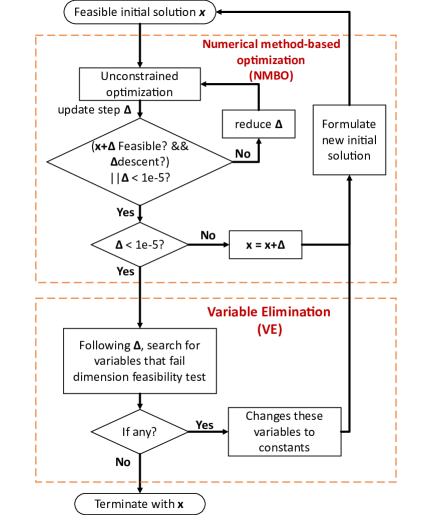
Figure 1: NORTH framework and components overview:
NMBO: Beginning with a feasible solution x, NORTH first utilizes trust-region methods to find an update direction $\boldsymbol{\Delta}$ for the optimization problem without the schedulability constraints. If $\boldsymbol{\Delta}$ leads x into an infeasible region, then $\boldsymbol{\Delta}$ is kept decreased until $\textbf{x}+\boldsymbol{\Delta}$ is feasible.
VE: After NMBO terminates, we check whether there are close active constraints. If so, the involved variables are transformed into constants in future iterations. The algorithm terminates when there are no more variables to optimize.

IV Numerical method-Based Optimization

IV-A Motivation

This section introduces a Numerical Method-Based Optimization (NMBO) algorithm to address the challenge of non-differentiable schedulability constraints. Leveraging active-set methods (ASM) and trust-region methods (TRM), NMBO allows temporarily “ignoring” inactive constraints during iterations, thereby avoiding analyzing gradients of the non-differentiable schedulability constraints in many cases.

The flowchart of NMBO is shown in figure 1. Each iteration begins with a feasible solution $\textbf{x}^{(k)}$ and performs unconstrained optimization to obtain an update step $\boldsymbol{\Delta}$. It then verifies whether $\textbf{x}^{(k)}+\boldsymbol{\Delta}$ is feasible and improves $\mathcal{F}(\textbf{x}^{(k)})$. If so, $\boldsymbol{\Delta}$ is accepted; otherwise, we decrease $\boldsymbol{\Delta}$ based on trust-region algorithms[14]. Finally, NMBO will terminate at either a stationary point (i.e., points with zero gradients) or feasible region boundaries.

In our experiments, Levenberg-Marquardt algorithm [44, 24] (LM), one of the classical trust-region algorithms, is used as the unconstrained optimizer. LM updates iterations with the following formula:

$$(\textbf{J}^{(k)T}\textbf{J}^{(k)}+\lambda\ \text{diag}(\textbf{J}^{(k)T}\textbf{J}^{(k)}))\boldsymbol{\Delta}=-\textbf{J}^{(k)T}\boldsymbol{\mathcal{F}}(\textbf{x}^{(k)})$$ (19)

where $\textbf{J}^{(k)}$ is the Jacobian matrix after linearizing the objective function (1). We can control the parameter $\lambda$ in Equation (19) to change the length of $\boldsymbol{\Delta}$. For example, larger $\lambda$ implies smaller $\boldsymbol{\Delta}$.

IV-B Numerical Gradient

Numerical gradients can be calculated as follows when the analytical gradient cannot be derived (e.g., black-box objective functions):

$$\frac{\partial\mathcal{F}_{i}(\textbf{x})}{\partial\textbf{x}_{i}}=\frac{\mathcal{F}_{i}(\textbf{x}_{1},..,\textbf{x}_{i}+h,..,\textbf{x}_{N})-\mathcal{F}_{i}(\textbf{x}_{1},..,\textbf{x}_{i}-h,..,\textbf{x}_{N})}{2h}$$ (20)

where $h=10^{-5}$ in our experiments, more consideration on how to choose $h$ can be found in Nocedal et al. [14]. The numerical gradients should be used with caution because we often observe that:

Observation 1.

Numerical gradient (20) at non-differentiable points could be a non-descent vector or lead to a non-feasible solution.

$\textbf{Justification}.\$ This is because the exact gradient at non-differentiable points is not well-defined and, therefore, is sensitive to many factors, such as the choice of $h$.

Observation 2.

Gradient-based constrained optimizers may terminate at infeasible solutions if the constraints are not differentiable.

$\textbf{Justification}.\$ This is because the numerical gradient of non-differentiable constraints is not reliable.

NMBO overcomes the challenges above by constructing local approximation models exclusively for objective functions rather than constraints. This is because schedulability constraints frequently lack differentiability, while the objective functions may not. If the objective function contains non-differentiable components, we use $0$ for its numerical gradient instead. After obtaining a descent vector $\boldsymbol{\Delta}$, NMBO accepts it only if $\textbf{x}^{(k)}+\boldsymbol{\Delta}$ is feasible. Therefore, NMBO guarantees to find feasible results while maintaining the speed advantages of classical gradient-based optimization algorithms.

IV-C Termination Conditions for NMBO

NMBO will terminate if the relative difference in the objective function

$$\delta_{\text{rel}}=\frac{\mathcal{F}(\textbf{x}^{(k+1)})-\mathcal{F}(\textbf{x}^{(k)})}{\mathcal{F}(\textbf{x}^{(k)})}$$ (21)

becomes very small, e.g., $\delta_{\text{rel}}\leq 10^{-5}$. NMBO will also terminate if the number of iterations exceeds a certain number (e.g., $10^{3}$).

Example 1.

Let’s consider a simplified energy minimization problem:

$$\min_{\textbf{c}_{1},\textbf{c}_{2}}\ (8\textbf{c}_{1}^{-1})^{2}+(\textbf{c}_{2}^{-1})^{2}$$ (22)

subject to $$\text{Sched}(\textbf{c}_{1},\textbf{c}_{2})=0$$ (23)

$$4\leq\textbf{c}_{1}\leq 10$$ (24)

$$1\leq\textbf{c}_{2}\leq 10$$ (25)

where the WCET of each task are the variables.

The task set includes two tasks: task 1 and task 2. Task 1’s initial execution time, period, and deadline are $\{4,10,6\}$, respectively; Task 2’s initial execution time, period, and deadline are $\{1,40,40\}$, respectively; Task 1 has a higher priority than task 2. The schedulability analysis is based on Equation (14) and (15).

Let’s consider an initial solution $\textbf{c}^{(0)}=(4,1)$. We use LM to perform unconstrained optimization, and use $10^{3}$ as the initial $\lambda$ in equation (19), then we can perform one iteration as follows:

$$\textbf{J}^{(0)}=\begin{bmatrix}-8/4^{2}&0\\ 0&-1/1^{3}\end{bmatrix}=\begin{bmatrix}-0.5&0\\ 0&-1\end{bmatrix}$$ (26)

$$\textbf{c}^{(1)}=\textbf{c}^{(0)}+\boldsymbol{\Delta}=\begin{bmatrix}4.004&1.001\end{bmatrix}$$ (27)

Multilpe iterations will be performed until $\textbf{c}^{(k)}$ becomes close to violating the schedulability constraints, e.g., $(5.999,1.499)$. At this point, NMBO cannot make big progress further without violating the schedulability constraints and so will terminate.

Observation 3.

The schedulability analysis process in an iterative algorithm such as NMBO can often be sped up if it can utilize a “warm start”.

$\textbf{Justification}.\$ Iterative algorithms typically make progress incrementally, which is beneficial for improving runtime speed in various schedulability analyses. For instance, consider the classical response time analysis (14). After the execution time $\textbf{c}_{i}$ of $\tau_{i}$ increases to $\textbf{c}_{i}+\boldsymbol{\Delta}_{i}$ where $\boldsymbol{\Delta}_{i}>0$, $r_{i}(\textbf{c}_{i})$ could be a warm start to analyze $r_{i}(\textbf{c}_{i})+\boldsymbol{\Delta}_{i}$ during the fixed-point iterations. Please check Davis et al. [45] to learn more about this topic.

V Variable Elimination

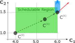
Figure 2: Variable elimination motivating example. Consider the problem in Example 1 and assume NMBO terminates at $(5.999,1.499)$. The red arrow shows the update step $\boldsymbol{\Delta}$ from classical unconstrained optimizers. Moving toward the red arrow will make task 1 miss its deadline. However, we can improve $\textbf{c}^{(k)}$ without violating the schedulability constraints by only updating $\textbf{x}_{2}$ following $\boldsymbol{\Delta}$ while leaving $\textbf{x}_{1}$ unchanged.

V-A Motivation and Definitions

There are usually chances to improve performance further after NMBO terminates. Figure 2 shows an example from Example 1, where a feasible update direction (blue) is hidden in an infeasible descent vector $\boldsymbol{\Delta}$ (red). Therefore, it is possible to optimize a subset of variables that will not immediately violate constraints, thereby enhancing the objective function. We call this simple idea variable elimination (VE).

To that end, detecting the feasible region’s boundary during iterations is important. This is not easy for the binary schedulability analysis constraint, which only returns true or false results. Early work [46, 47] usually assumes a specific form of schedulability analysis and so cannot work with Equation (6). The classical definition of active constraints introduced in Section III-B is also unsuitable because it is defined for continuous functions. Therefore, we generalize the definition of active constraints for the binary schedulability analysis:

Definition V.1 (Active schedulability constraint).

A binary schedulability constraint, equation (6), is an active constraint at a point $\textbf{x}^{*}$ if:

$$\text{Sched}(\textbf{x}^{*})=0$$ (28)

$$\exists\boldsymbol{\delta},\|\boldsymbol{\delta}\|\leq h,\text{Sched}(\textbf{x}^{*}+\boldsymbol{\delta})=1$$ (29)

where $h>0$ is the numerical granularity.

In other words, if a schedulability constraint is active at $\textbf{x}^{*}$, that means $\textbf{x}^{*}$ is schedulable but is close to becoming unschedulable.

Upon termination of NMBO, some constraints may become active constraints and prevent NMBO from making progress. One potential solution is removing these active constraints from the optimization problem. However, we must also guarantee that the final solutions respect these active constraints. Therefore, we can find the variables involved in the active constraints, lock their values from future optimization, and then safely ignore these active constraints in future iterations. Based on Definition V.1, we can find these variables based on the following method:

Definition V.2 (Dimension feasibility test).

A solution $\textbf{x}\in\mathbb{R}^{N}$ for problem (5) passes dimension-j feasibility test of length d along the direction $\boldsymbol{\Delta}$ if $\textbf{x}\oplus(\frac{\boldsymbol{\Delta}_{j}}{|\boldsymbol{\Delta}_{j}|}d,j)$ is feasible, with $j\in[0,N-1]$.

where the $\oplus$ operation for vectors x and y is defined as follows:

$$\textbf{y}=\textbf{x}\oplus(d,j)\ \Leftrightarrow\ \textbf{y}_{i}=\begin{cases}\textbf{x}_{i},&i\neq j\\ \textbf{x}_{i}+d&i=j\end{cases}$$ (30)

In simpler terms, a variable, $\textbf{x}_{i}$, should be eliminated if it fails the dimension-$i$ feasibility test along $\boldsymbol{\Delta}$ of length $d\geq h$, where the descent direction $\boldsymbol{\Delta}$ is given by unconstrained optimizers. After eliminating $\textbf{x}_{i}$ at $\textbf{x}^{(k)}$, its value will always be the same as $\textbf{x}^{(k)}_{i}$. Section V-D will introduce an adaptive strategy to find the elimination tolerance $d$.

Example 2.

Let’s continue with Example 1 and first consider an elimination tolerance $d=10^{-5}$. Following Definition V.2, $\textbf{c}^{(k)}$ passes dimension-1 (with $\textbf{c}_{1}$) and dimension-2 (with $\textbf{c}_{2}$) feasibility test. This is because both $(5.999+10^{-5},1.499)$ and $(5.999,1.499+10^{-5})$ are feasible. If $d=10^{-1}$, $\textbf{c}^{(k)}$ will fail the dimension-1 feasibility test (with $\textbf{c}_{1}$) but still pass the dimension-2 feasibility test (with $\textbf{c}_{2}$).

V-B Theoretical Analysis of Variable Elimination

The design metrics in many real-time systems are decoupled. This means that the metric is assessed for each task individually, where a set of variables are provided by each task, such as the problems described in Section III-D and III-E. The decoupled systems are useful because of the nice properties shown next:

Definition V.3 (Strict descent step).

At x, an update step $\boldsymbol{\Delta}\in\mathbb{R}^{N}$ is a strict descent step if

$$\forall i\in[0,N-1],\ \mathcal{F}(\textbf{x}\oplus(\boldsymbol{\Delta}_{i},i))\leq\mathcal{F}(\textbf{x})$$ (31)

Observation 4.

If $\mathcal{F}(\textbf{x})=\sum_{i=0}^{N-1}\mathcal{F}_{i}(\textbf{x}_{i})$ is differentiable at $\hat{\textbf{x}}$, then there exists $\alpha>0$ such that $\boldsymbol{\Delta}=-\alpha\boldsymbol{\nabla}\mathcal{F}$ is often a strict descent step.

$\textbf{Justification}.\$ This is based on Taylor expansion:

$$\forall i,\exists\alpha>0,\mathcal{F}(\hat{\textbf{x}}\oplus(\boldsymbol{\Delta}_{i},i)) \approx\mathcal{F}(\hat{\textbf{x}})+\boldsymbol{\Delta}_{i}\boldsymbol{\nabla}\mathcal{F}_{i}(\hat{\textbf{x}}_{i})$$

$$=\mathcal{F}(\hat{\textbf{x}})-\alpha(\boldsymbol{\nabla}\mathcal{F}_{i}(\hat{\textbf{x}}_{i}))^{2}\leq\mathcal{F}(\hat{\textbf{x}})$$

Next, we introduce extra symbols for the theorems below. At a feasible point $\textbf{x}\in\mathbb{R}^{N}$, $\boldsymbol{\Delta}\in\mathbb{R}^{N}$ denotes a descent direction provided by an unconstrained optimizer. Notice that $\boldsymbol{\Delta}\in\mathbb{R}^{N}$ may not be a feasible direction. $\boldsymbol{\mathcal{S}}$ denotes the set of dimension indexes $i$ that pass the dimension-$i$ feasibility test with length $d\geq h$ along $\boldsymbol{\Delta}$.

We use $\bar{\boldsymbol{\mathcal{S}}}$ to denote the set of indices that fail the test. Within the context of a dimension-i feasibility test and an update step $\boldsymbol{\Delta}$, we also introduce a vector ${\textbf{v}}_{i}^{\mathcal{D}}\in\mathbb{R}^{N}$ where its ${j}^{\textit{th}}$ element is given as follows:

$${\textbf{v}}_{i,j}^{\mathcal{D}}=\begin{cases}\boldsymbol{\Delta}_{j}&j=i\\ 0&\text{otherwise}\end{cases}$$ (32)

Theorem 1.

If $\boldsymbol{\Delta}$ is a strict descent step, and $|\boldsymbol{\boldsymbol{\mathcal{S}}}|=q>0$, then all the ${\textbf{v}}_{i}^{\mathcal{D}}$ are feasible descent vectors at x.

Proof.

Results of Definition V.3 and Theorem 4. ∎

Theorem 2.

If both the objective function $\mathcal{F}(\textbf{x})$ and the constraints in the optimization problem (5) are differentiable at $\textbf{x}^{(k)}$, and $|\boldsymbol{\mathcal{S}}|=q>0$, then there exists $\bar{d}<d$ such that $\textbf{x}^{(k)}+\boldsymbol{\hat{\Delta}}$ is feasible with no worse objective function values:

$$\boldsymbol{\hat{\Delta}}\in\{ \sum_{i}^{q}\alpha_{i}\textbf{v}_{i}^{\mathcal{D}}\ |\ \|\boldsymbol{\hat{\Delta}}\|_{1}\leq\bar{d},\ \alpha_{i}\geq 0\}$$ (33)

$$\mathcal{F}(\textbf{x}^{(k)}+\boldsymbol{\hat{\Delta}})\leq\mathcal{F}(\textbf{x}^{(k)})$$ (34)

Proof.

The theorem can be proved by applying the Taylor expansion to the objective functions and constraints. ∎

Although the objective functions and schedulability constraints in real-time systems are not differentiable everywhere in $\mathbb{R}^{N}$, VE is still useful because there are many differentiable points x. Actually, if we randomly sample a feasible point $\textbf{x}\in\mathbb{R}^{N}$, x is more likely to be a differentiable point than a non-differentiable point because there are only limited non-differentiable points but infinite differentiable points. During the optimization iterations, if $\textbf{x}^{(k)}$ is a differentiable point, then Theorem 2 states that VE can find a descent and feasible update direction to improve $\textbf{x}^{(k)}$.

V-C Generalization to Non-differentiable Objective Function

In cases that NMBO terminates at a non-differentiable point $\textbf{x}^{(k)}$, we can generalize the dimension feasibility test (Definition V.2) as follows:

Definition V.4 (Dimension feasibility descent test).

A solution $\textbf{x}\in\mathbb{R}^{N}$ for optimization problem (5) passes dimension-j feasibility descent test of length d along the direction $\boldsymbol{\Delta}$ if $\textbf{x}\oplus(\frac{\boldsymbol{\Delta}_{j}}{|\boldsymbol{\Delta}_{j}|}d,j)$ is feasible, where $j\in[0,N-1]$ and

$$\mathcal{F}(\textbf{x}\oplus(\frac{\boldsymbol{\Delta}_{j}}{|\boldsymbol{\Delta}_{j}|}d,j))\leq\mathcal{F}(\textbf{x})$$ (35)

It is useful in scenarios where non-sustainable response time analysis is included in the objective function.

V-D Performing Variable Elimination

Theorem 2 suggests that $\textbf{x}^{(k)}$ can be improved by gradient-based optimizers if $\textbf{x}_{\bar{\boldsymbol{\mathcal{S}}}}$ are transformed into constant values at $\textbf{x}^{(k)}$. This idea can be implemented following Algorithm 1.

The elimination tolerance $d$ is found by first trying small values (e.g., the numerical granularity $h$). If no variables are eliminated, we can keep increasing $d$ (for example, 1.5x each time) until we can eliminate at least one variable.

Input: $\textbf{x}^{(k)}$, descent step $\boldsymbol{\Delta}$, elimination tolerance $d$, un-eliminated indexes set $\boldsymbol{\mathcal{U}}$

Output: eliminated variable indexes

1 for $(i\ \textbf{in}\ \boldsymbol{\mathcal{U}})$ do

2       $\textbf{x}_{i}^{(k)}=\textbf{x}_{i}^{(k)}+d\frac{\boldsymbol{\Delta}_{i}}{|\boldsymbol{\Delta}_{i}|}$

3       if  (AnyConstraintIsViolated($\textbf{x}_{i}^{(k)}$) OR IsNonDifferentiable($\textbf{x}_{i}^{(k)}$)) then

4             return i

5       end if

       $\textbf{x}_{i}^{(k)}=\textbf{x}_{i}^{(k)}-d\frac{\boldsymbol{\Delta}_{i}}{|\boldsymbol{\Delta}_{i}|}$ // Recover $x_{i}^{(k)}$

6      

7 end for

Algorithm 1 Variable elimination

Example 3.

Let’s continue with Example 1 and see how to select $d$ and variables ($\textbf{c}_{1}$ or $\textbf{c}_{2}$) to eliminate. We can first try to increase $\textbf{c}_{1}$ and $\textbf{c}_{2}$ by $d=10^{-5}$ respectively but then find that no constraints are violated. Therefore, $d$ is kept being increased (1.5x each time) until $d=10^{-5}\times 1.5^{12}>0.001$. In this case, $\textbf{c}^{(k)}$ fails the dimension-1 feasibility test (with $\textbf{c}_{1}$) while still passing the dimension-2 feasibility test (with $\textbf{c}_{2}$). Hence, $\textbf{c}_{1}$ will be eliminated first. In future iterations, $\textbf{c}_{1}$ will be a constant 5.999, and $\textbf{c}_{2}$ will become the only variable left.

V-E Speed up variable elimination

We can speed up the process of finding eliminated variables for some schedulability analysis. Let’s denote the update step for $\textbf{x}_{i}$ as $\Delta=d\frac{\boldsymbol{\Delta}_{i}}{|\boldsymbol{\Delta}_{i}|}$ in Algorithm 1.

Theorem 3.

If an variable $\textbf{x}_{i}$ is eliminated at a feasible point x, and there exists another variable $\textbf{x}_{j}$ that has bigger influence than $\textbf{x}_{i}$ in terms of schedulability, which means:

$$\text{Sched}(..,x_{j},..,x_{i}+d\frac{\boldsymbol{\Delta}_{i}}{|\boldsymbol{\Delta}_{i}|},..)=1$$ (36)

$$\text{Sched}(..,x_{j}+d\frac{\boldsymbol{\Delta}_{j}}{|\boldsymbol{\Delta}_{j}|},..,x_{i},..)\geq\text{Sched}(..,x_{j},..,x_{i}+d\frac{\boldsymbol{\Delta}_{i}}{|\boldsymbol{\Delta}_{i}|},..)$$ (37)

and assume $\boldsymbol{\Delta}_{i}\boldsymbol{\Delta}_{j}\geq 0$. In this case, $\textbf{x}_{j}$ should also be eliminated.

Proof.

Based on Equation (36) and (37), $\textbf{x}_{j}$ satisfies the elimination conditions. ∎

Theorem 3 states that if we know some variables, denoted as $x_{j}$, have a bigger influence on schedulability than other variables, denoted $x_{i}$, then we can always first check whether the lower-influence variables $x_{i}$ need to be eliminated. If so, variables with bigger influence $x_{j}$ are known to be eliminated, and we can save extra iterations in NMBO and VE.

Although analyzing variables’ relative influence for black-box schedulability analysis is difficult, such analysis is possible for many famous schedulability analyses. For example, consider preemptive computation platforms where execution times are variables. The utility test for the earliest deadline first scheduling algorithm (tasks with lower periods have a bigger influence) and Equation (14) for the rate monotonic [48] scheduling algorithm are good examples.

Example 4.

As an example of Theorem 3, we consider the response time analysis (14) and use WCET c as the variables. In this case, $\textbf{c}_{i}$ of tasks with higher priority has a bigger influence in terms of schedulability. To see that, let’s assume c does not pass the dimension-$i$ feasibility test, denote $\tau_{k}$ as a task with higher priority than $\tau_{i}$, $r_{i}(\textbf{c}_{i},\textbf{c}_{k})$ as $\tau_{i}$’s response time. Then, there exists $\Delta>0$ such that

$$r_{i}(\textbf{c}_{i},\textbf{c}_{k})=\textbf{c}_{i}+\sum_{j\in\text{hp}(i)}\lceil\frac{r_{i}(\textbf{c}_{i},\textbf{c}_{k})}{T_{j}}\rceil{\textbf{c}_{j}}\leq D_{i}$$ (38)

$$r_{i}(\textbf{c}_{i}+\Delta,\textbf{c}_{k})=\textbf{c}_{i}+\Delta+\sum_{j\in\text{hp}(i)}\lceil\frac{r_{i}(\textbf{c}_{i}+\Delta,\textbf{c}_{k})}{T_{j}}\rceil{\textbf{c}_{j}}>D_{i}$$ (39)

Then, $\textbf{c}_{k}$ is guaranteed to be eliminated with $\textbf{c}_{i}$ because:

$$\begin{split}r_{i}(\textbf{c}_{i},\textbf{c}_{k}+\Delta)&=\textbf{c}_{i}+\sum_{j\in\text{hp}(i),j\neq k}\lceil\frac{r_{i}(\textbf{c}_{i},\textbf{c}_{k}+\Delta)}{T_{j}}\rceil{\textbf{c}_{j}}\\ &+\lceil\frac{r_{i}(\textbf{c}_{i},\textbf{c}_{k}+\Delta)}{T_{k}}\rceil{(\textbf{c}_{k}+\Delta)}\\ &\geq r_{i}(\textbf{c}_{i}+\Delta,\textbf{c}_{k})>D_{i}\end{split}$$ (40)

The “$\geq$” sign can be seen to hold by considering the process of fixed-point iteration and noting the following

$$\lceil\frac{r_{i}(\textbf{c}_{i},\textbf{c}_{k})}{T_{k}}\rceil{\Delta}\geq\Delta$$ (41)

V-F Termination Condition

The algorithm may terminate at a stationary point found by NMBO. However, in most cases, after NMBO terminates in each iteration, VE will find new variables to eliminate due to the schedulability constraints. Eventually, NORTH will terminate after all the variables are eliminated.

Theorem 4.

The number of iterations in NORTH is no larger than $N$, where $N$ is the number of variables.

Proof.

This is because the values of elimination tolerance $d$ are selected to guarantee that at least one variable will be eliminated in each iteration. ∎

Example 5.

In Example 3, after eliminating $\textbf{c}_{1}$ at $5.999$, $\textbf{c}_{2}$ becomes the only left variable. In the next iteration, NMBO will run and terminate at the schedulability boundary when $\textbf{c}_{2}=15.89$, where $\tau_{2}$’s response time $r_{2}=39.89<40$. The algorithm does not make further progress (e.g., terminate at $\textbf{c}_{2}=15.99$) because the relative error difference between the last two iterations in NMBO is already smaller than $10^{-5}$ when $\textbf{c}_{2}=15.89$.

After NMBO terminates, VE proceeds to find new variables for elimination. The elimination tolerance $d=10^{-5}\times 1.5^{12}$ from Example 3 is first tried but cannot eliminate any new variables. Therefore, we keep increasing $d$ until $d=10^{-5}\times 1.5^{23}>0.11$, where $\textbf{c}_{2}+d$ violates the scheduleability constraint. Therefore, $\textbf{c}_{2}$ is eliminated next. After that, there are no variables to optimize, and so NORTH will terminate at 5.999, 15.89, which is very close to the optimal solution (6, 16).

The idea of VE may be similar to gradient projection (GP). However, VE differs from GP by avoiding the expensive and complicated projecting process and instead using the much simpler heuristics from Definition V.2. Also, GP usually assumes the problem is differentiable, which is not required by VE.

Theorem 5.

Solutions found by North are always feasible.

Proof.

This can be seen by considering the iteration process shown in Figure 1: The initial solution is feasible; NMBO only accepts feasible updates, while VE does not change the values of variables. Besides, all the constraints are kept and remain unchanged throughout the iterations. Therefore, the theorem is proved. ∎

V-G Discussion and Limitations of Variable Elimination

VE is useful when there are active scheduling constraints. In real-time system optimization, the optimal solution is often near the boundary of the schedulable region, and VE is therefore often helpful.

Another way to view VE is that variables usually have different sensitivity to schedulability constraints. Therefore, we must differentiate these variables (by dimension feasibility test) and make distinct adjustments (by variable elimination and NMBO). In this case, VE finds the variables far from violating the schedulability constraints and allows the unconstrained optimizers to optimize these variables further.

VE sacrifices the potential performance improvements associated with the eliminated variables. However, exploiting these potential performance improvements could be complicated and computationally expensive (e.g., projected gradients, see more in Noccedal et al. [14]). Besides, the potential performance improvements are likely to be limited because NORTH showed close-to-optimal performance in experiments.

VI Hybrid optimization

VI-A Framework Overview

In this section, we generalize NORTH to NORTH+, which supports collaborative optimization of continuous and discrete variables. The overview of NORTH+ is shown in figure 3, where we adopt an iterative framework to optimize the continuous and discrete variables separately. This is inspired by the coordinate-descent algorithm [49]. When optimizing continuous variables, the discrete variables are treated as constant. Similarly, the continuous variables are treated as constant when optimizing the discrete variables. Although NORTH can optimize the continuous variables, an algorithm to optimize the discrete variables is required for NORTH+ to work.

This section uses priority assignments as the discrete variables and introduces a new algorithm to perform priority assignments guided by numerical optimization algorithms. The algorithm is based on the following observation:

Observation 5.

After increasing a task $\tau_{i}$’s priority, its worst-case response time $r_{i}$ usually will not become longer.

Although not always true, the observation above establishes a monotonic relationship between priority assignments and response time. Furthermore, since response times are continuous variables, we can first treat response time r as variables, obtain an update step $\boldsymbol{\Delta}\textbf{r}$, and then adjust priority assignments to make $\boldsymbol{\Delta}\textbf{r}$ happen.

VI-B Problem description

For the convenience of presentation, we restate the hybrid optimization problem considered in this section:

$$\min_{\textbf{x},\textbf{P}}\ \ \ \ \ \mathcal{F}(\textbf{x},\textbf{r})$$ (42)

subject to $$\ \textbf{r}=\boldsymbol{\mathcal{G}}(\textbf{x},\textbf{P})$$ (43)

$$\ \forall\tau_{i}\in\boldsymbol{\tau},\textbf{r}_{i}\leq D_{i}$$ (44)

$$\ \text{lb}_{i}\leq\textbf{x}_{i}\leq\text{ub}_{i},i\in[0,N-1]$$ (45)

where x are continuous variables that represent the design choices, such as the execution times or periods of tasks (Assumption 2); The priority assignments P for a task set $\boldsymbol{\tau}$ are described by an ordered sequence of all the tasks. Tasks that appear earlier in the sequence have higher priority. The response time analysis function $\boldsymbol{\mathcal{G}}(\textbf{x},\textbf{P})$ is a black-box function that depends on x and P.

An example application is given in Section III-E.

Example 6.

A priority assignment vector $\textbf{P}=\{\tau_{1},\tau_{2},\tau_{0}\}$ denotes that $\tau_{1}$ has the highest priority, $\tau_{0}$ has the lowest priority.

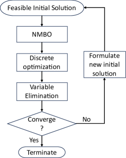
Figure 3: Overall optimization framework NORTH+. The NMBO and VE components are shown in figure 1, and the discrete optimization step is introduced in this section.

VI-C Optimize the Response Time Vector

The hybrid optimization problem (42) is transformed into an unconstrained optimization problem as follows:

$$\min_{\textbf{P}}\mathcal{Z}(\textbf{r}|\textbf{x})=\mathcal{F}(\textbf{r}|\textbf{x})-w\sum_{\tau_{i}\in\boldsymbol{\tau}}\textbf{Barrier}(D_{i}-\textbf{r}_{i}))$$ (46)

where $\mathcal{F}(\textbf{r}|\textbf{x})$ denote that x is treated as a constant in the function, $w>0$ controls the relative importance of the barrier function [50]:

$$\textbf{Barrier}(x)=\begin{cases}\log(x),&x>0\\ -\infty,&\text{otherwise}\end{cases}$$ (47)

The transformed objective function above is safe because a good solver minimizes the objective function, avoiding unschedulable situations.

The gradient evaluation of the objective function (46) with respect to the response time r is given as follows:

$$\boldsymbol{\nabla}_{\textbf{r}}\mathcal{Z}=\boldsymbol{\nabla}_{\textbf{r}}\mathcal{F}(\textbf{x},\textbf{r})-w\sum_{\tau_{i}\in\boldsymbol{\tau}}\frac{1}{D_{i}-\textbf{r}_{i}}$$ (48)

A simple way to update the response time is by following the gradient descent algorithm:

$$\boldsymbol{\Delta r}=-\alpha\boldsymbol{\nabla}_{\textbf{r}}$$ (49)

where $\alpha>0$ is decided as in the typical gradient descent algorithms. More sophisticated methods such as LM (Equation (19)) can also be used,

VI-D Optimize Priority Assignments

Given an initial feasible priority assignment, this section presents a heuristic algorithm to adjust priority assignments to optimize $\mathcal{Z}(\textbf{r}|\textbf{x})$ following $\boldsymbol{\Delta r}$. The hope is that we can change $\textbf{r}^{(k)}$ into $\textbf{r}^{(k)}+\boldsymbol{\Delta r}$ as much as possible by adjusting priority assignments $\textbf{P}^{(k)}$.

The priority assignments are adjusted in an iterative way where we change one task’s priority each time. At first, all the tasks are pushed into a set $\boldsymbol{\mathcal{S}}^{todo}=\boldsymbol{\tau}$, which contains the tasks waiting to adjust priority assignments. Within each iteration, we pick up one task from $\boldsymbol{\mathcal{S}}^{todo}$ and try to increase its priority until doing so cannot improve the objective function. The pseudocode of this idea is shown in Algorithm 2. The function in line 4 is introduced in section VI-E.

Input: $\textbf{x}^{(k)}$, gradient $\boldsymbol{\nabla}_{\textbf{r}}\mathcal{Z}$, current objective function value $F^{(k)}$, priority assignments $\boldsymbol{P}^{(k)}$

Output: $\boldsymbol{P}^{(k+1)}$

1 $\boldsymbol{\mathcal{S}}^{todo}=\boldsymbol{\tau}$

2

3while $\boldsymbol{\mathcal{S}}^{todo}\neq\emptyset$  do

4       $\tau_{i}$ = PickTaskWithPotential($\boldsymbol{\mathcal{S}}^{todo}$, $\boldsymbol{\nabla}_{\textbf{r}}\mathcal{Z}$)

5       if $\tau_{i}$ has potential then

6             while true do

7                   $\boldsymbol{P}$ = IncreasePriority($\boldsymbol{P}^{(k)}$, $\tau_{i}$ )

8                   if $\mathcal{F}$(x, r(x, $\boldsymbol{P}$)) $<$ $F^{(k)}$ then

9                         $\boldsymbol{P}^{(k)}$ = $\boldsymbol{P}$

10                        

11                  else

12                        break

13                   end if

14                  

15             end while

16            

17       end if

18      Pop($\boldsymbol{\mathcal{S}}^{todo}$, $\tau_{i}$)

19 end while

$\boldsymbol{P}^{(k+1)}=\boldsymbol{P}^{(k)}$

Algorithm 2 Optimize priority assignments

VI-E How to select tasks to increase its priority?

If the schedulability analysis is time-consuming, Algorithm 2 may waste lots of time performing unnecessary schedulability analysis. Therefore, we propose two heuristics to decide how to select tasks that can improve the objective function.

We first introduce some notations. We use $\textbf{P}^{(k)}$ to denote the priority assignment at ${k}^{\textit{th}}$ iteration, use $\textbf{P}^{G}$ to denote a priority assignment vector from $\boldsymbol{\nabla}_{\textbf{r}}\mathcal{Z}^{(k)}$ where tasks with bigger gradient have higher priority.

Given a priority assignment vector P, $\textbf{P}(i)$ denotes the priority order of the task $\tau_{i}$. For example, the highest priority task’s priority order is 1, and the lowest priority task’s priority order is $N$ if there are $N$ tasks.

Example 7.

Let’s consider the task set in Example 1 except that we are optimizing task periods with the following objective function

$$\min_{\textbf{T},\textbf{P}}T_{1}+T_{2}+r_{1}(\textbf{T},\textbf{P})+r_{2}(\textbf{T},\textbf{P})$$ (50)

Furthermore, consider a variable at ${k}^{\textit{th}}$ iteration where $\textbf{T}^{(k)}_{1}=10,\textbf{T}^{(k)}_{2}=6$. When optimizing the period variables, we assume that the system follows the implicit deadline policy, which means that the deadline is always the same as the period variable. The initial priority vector $\textbf{P}^{(k)}=\{1,2\}$, which means task 1 has a higher priority than task 2.

Assume the weight parameter $w$ in objective function (46) is $1$, then we have $\textbf{r}_{1}=4,\textbf{r}_{2}=5$, $\boldsymbol{\nabla}_{\textbf{r}}\mathcal{Z}^{(k)}=[1.25,2]^{T}$, $\textbf{P}^{G}(1)=2$, $\textbf{P}^{G}(2)=1$.

Observation 6.

Increasing a task $\tau_{i}$’s priority is more likely to improve the objective function if $\textbf{P}^{G}(i)<\textbf{P}^{(k)}(i)$

$\textbf{Justification}.\$ The basic idea of the algorithm is that a task with a bigger gradient should be assigned with a higher priority because it has more influence on the objective function. Therefore, a task with a small gradient should not be assigned with higher priority.

Example 8.

Continue with Example 7. There is no need to increase task 1’s priority even if task 1 does not have the highest priority because its gradient is smaller than task 2’s.

Observation 7.

If increasing the priority of a task $\tau_{i}$ from its current priority $j$ fails to improve the objective function, then it is highly likely that the same will hold even if other tasks’ priority assignments change in future iterations.

The second observation can be implemented via a hash map, which records the number of failed priority adjustments for task $\tau_{i}$ when assigned the ${j}^{\textit{th}}$ highest priority. If the failed adjustments exceed a threshold (1 in our experiments), then we will not try to increase $\tau_{i}$’s priority when it is at $j$.

VI-F Encourage convergence

The weight parameter $w$ in the objective function (46) can be set up following the classical interior point method. The initial $w$ parameter could have a relatively large value ($10^{7}$ in our experiments); $w$ decreases by half after finishing one iteration every time. Eventually, $w$ will converge to 0 such that the transformed objective function (46) will converge to the actual objective function.

VII Run-time complexity estimation

The run-time complexity of NORTH is analyzed as follows:

$$\text{Cost}_{NORTH}=N_{\text{Elimi}}\times(\text{Cost}_{\text{TR}}+\text{Cost}_{\text{Elimi}})$$ (51)

where $N_{\text{Elimi}}$ denotes the number of elimination loops, $\text{Cost}_{\text{TR}}$ denotes the cost of the trust-region optimizer, and $\text{Cost}_{\text{Elimi}}$ denotes the cost of variable elimination. Let’s use $N$ to denote the number of variables and analyze each of these terms.

Firstly, following Theorem 4, we have

$$N_{\text{Elimi}}\leq N$$ (52)

Let’s use $\text{Cost}_{\text{sched}}$ to denote the cost for schedulability analyses, $\text{N}_{\text{TR}}$ for the number of trust-region iterations, then:

$$\text{Cost}_{\text{TR}}\leq N_{\text{TR}}\times(\text{Cost}_{\text{sched}}+O(N^{3}))$$ (53)

where $\text{N}_{\text{TR}}$ mostly is decided by the convergence rate of the gradient-based optimizer, which is often very fast, e.g., super-linear or quadratic convergence rate [14]. The $O(N^{3})$ term above denotes the cost of matrix computation.

As for the last term in Equation (51):

$$\text{Cost}_{\text{Elimi}}\leq N\times\text{Cost}_{\text{sched}}$$ (54)

The run-time complexity of NORTH+ has an extra term regarding adjusting priority assignments:

$$\text{Cost}_{NORTH+}=\text{Cost}_{NORTH}+N_{\text{Elimi}}\times O(N^{2})\times\text{Cost}_{Sched}$$ (55)

where we have the $N^{2}$ term because each task’s priority can only be increased at most $N$ times.

VIII Application and generalizations

In this section, we discuss how to relax the two assumptions 1 and 2 and limitations.

VIII-A Finding feasible initial solutions

The optimization variables in real-time systems usually have semantic meanings. In these cases, feasible initial solutions can be found by setting them the values that are more likely to be schedulable, e.g., the shortest execution time/longest period. This method is optimal in finding initial solutions if the schedulability analyses are sustainable, such as the schedulability analysis based on the response time analysis (14). Please see more results in Section IX-E.

Alternatively, the feasible initial solution can be found by solving a phase-1 optimization problem [50]. This method is applicable when the influence of violating schedulability constraints can be obtained quantitatively. For example, tardiness, which measures the additional time tasks require for completion beyond specified deadlines. In this case, we can first solve a phase-1 problem, which minimizes the sum of barrier functions of all the tasks. For each task $\tau_{i}$, denote its deadline and worst-case response time as $D_{i}$ and $r_{i}$, the barrier function is defined as follows:

$$\text{Barrier}(D_{i}-r_{i})=\begin{cases}0&D_{i}\geq r_{i}\\ -(D_{i}-r_{i})&D_{i}<r_{i}\end{cases}$$ (56)

The barrier function is expected to reduce to zero after optimization. If so, a feasible initial solution is obtained.

VIII-B Optimizing Categorical Variables

NORTH can optimize categorical variables if there is a rounding strategy to transform these variables into and back continuous variables. Variables that satisfy such requirements could be integer periods or run-time frequencies that can only be selected within a discrete set. In these cases, performing variable rounding is usually not difficult. For example, if all the constraints are monotonic (in cases of schedulability constraints, that means they are sustainable), we can round floating-point variables into integers as follows: If rounding down the variable does not adversely affect system schedulability, we may do so to ensure schedulability; otherwise, we round it up.

One potential issue is that some schedulability analyses may only accept categorical variables, such as when optimizing the periods (usually not float-point numbers) [6]. In this case, we must round the float-point solution into discrete variables before performing the schedulability analysis. This method is used in the NORTH+ experiment in Section IX-C.

VIII-C Limitations

NORTH relies on the gradient information from the objective function to utilize the gradient-based optimizers. For example, if $\alpha_{i}=0$ for all the $i$ in the objective function (16), then the gradient of (16) with respect to the period variables would be either 0 or undefined. In this case, NORTH probably cannot make any progress. Another limitation is that NORTH usually cannot guarantee to find global optimal solutions since it relies on gradient-based optimizers.

IX Experiments

NORTH and NORTH+ are implemented in C++, where the numerical optimization algorithms are provided by a popular library GTSAM[51] in the robotics area [52, 53, 54, 55]. We perform the experiments on a desktop (Intel i7-11700 CPU, 16 GB Memory) with the following baseline methods:

• Zhao20, from [10]. It requires the schedulability analysis to be sustainable to be applicable. If not time-out, it finds the optimal solution.

• MIGP, mixed-integer geometric programming. The MIGP is solved by gpposy[56] with BnB solver in YALMIP[57].

• IPM, a famous constrained optimization method [14]. It is implemented with IFOPT and IPOPT [58, 59]. Numerical gradients are used in experiments to be applicable.

• NMBO, introduced in Section IV.

• NORTH, the optimization framework shown in figure 1.

• SA, simulated annealing. The cooling rate is 0.99, the temperature is $10^{5}$, and the iteration limit is $10^{6}$.

LM (19) is the unconstrained optimizer in all the NORTH-related methods. There is a time limit of 600 seconds for each method. We use the initial solution during performance evaluation if a baseline method cannot find a feasible solution within the time limit. Some methods are not shown in the figures because they are not applicable or require too much time to run.

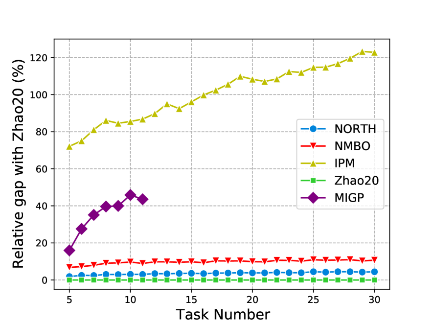
(a) DVFS performance with FTP Scheduling

(b) DVFS performance with DAG [6]

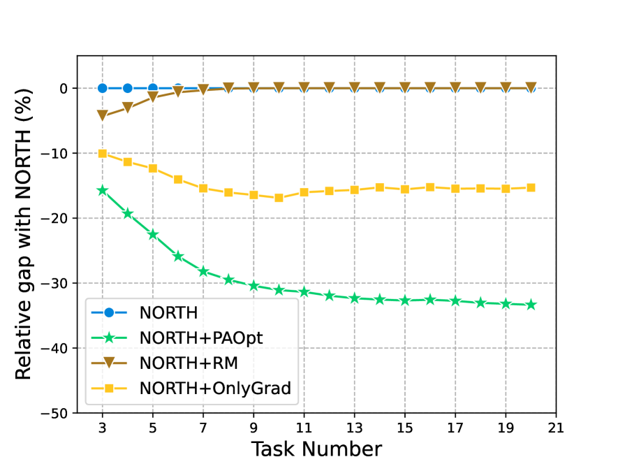
(c) Hybrid control performance optimization

(d) DVFS log run-time with FTP Scheduling

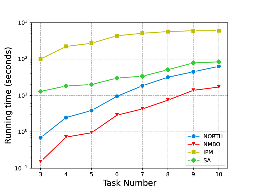
(e) DVFS log run-time with DAG [6]

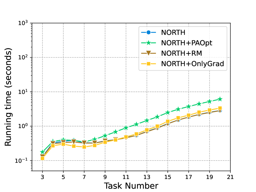
(f) Hybrid control optimization log run-time

Figure 4: The performance and run-time speed of the experiments.

IX-A Energy Optimization based on FTP Model

In this experiment, we adopted the same settings as in Zhao et al. [10] for the convenience of comparison. The objective function is simplified as follows:

$$E_{i}(\textbf{f})=\frac{H}{T_{i}}(\alpha\textbf{f}_{i}^{3})\times(\frac{c_{i}^{\text{org}}}{\textbf{f}_{i}})$$ (57)

where $c_{i}^{\text{org}}$ denotes the WCETs for $\textbf{f}_{i}=1$.

We generate the task sets randomly as follows. The task set’s utilization was randomly generated from $0.5$ to $0.9$. For each task, its period was selected from a log-uniform distribution from $10^{2}$ to $10^{5}$; its utilization was generated using Uunifast [45]; its run-time frequency is lower-bounded by half of its initial value; its deadlines were the same as its period; its priorities were assigned based on the Rate Monotonic (RM) policy. The response time analysis (14) and equation (15) provide the schedulability constraints.

In Figure 4(a), the relative gap between a baseline method and Zhao20 is defined as follows:

$$\frac{E_{\text{baseline}}-E_{\text{Zhao20}}}{E_{\text{Zhao20}}}\times 100\%$$ (58)

IX-B Energy Optimization for DAG Model

In the second experiment, we consider the exact optimization problem (9) where the schedulability analysis is provided by Nasri et al. [6]. The schedulability analysis considers a task set whose dependency is modeled by a directed acyclic graph (DAG). The task set is executed on a non-preemptive multi-core computation platform. The schedulability analysis is not sustainable with respect to either tasks’ worst-case execution time or periods. Therefore, MIGP or Zhao20 cannot be applied to solve this problem.

The simulated task sets were generated randomly, where each task set contained several periodic DAG tasks. We generate the DAG structures following [60], which randomly added an edge from one node to another with a probability (0.2 in our experiments). The number of nodes within each DAG follows a uniform distribution between 1 and 20. Nodes of the same DAG have the same period. The period of each DAG was randomly selected according to a popular automotive benchmark [8] in the literature [61, 62]. Considering the current schedulability analysis is time-consuming, the actual periods were randomly selected within a sub-set: $\{1,2,5,10,20,50,100\}$. The number of DAGs, $N$, in each task set ranges from 3 to 10. For each $N\in[3,10]$, 105 task sets were generated, where 15 task sets were generated for each total utilization ranging from $0.1\times 4$ to $0.9\times 4$. All the task sets were assumed to execute on a homogeneous 4-core computing platform. The utilization of each DAG within a task set and the execution time of each node are all generated with a modified Uunifast [45] algorithm, which makes sure that each DAG/node’s utilization is no larger than 100$\%$. During optimization, the relative error tolerance is $10^{-3}$, and the initial elimination tolerance is 10.

The execution time of all the nodes of all the DAGs are the optimization variables. When $N=10$, there were 100 nodes on average to optimize, 200 nodes at most. Figure 4(b) and figure 4(e) show the results, where the relative performance gap is calculated against the initial energy consumption.

IX-C Control Performance Optimization

Our third experiment considers the control performance optimization problem in Section III-E. This problem is more challenging because the objective function contains non-differentiable response time functions; furthermore, both continuous variables (periods) and discrete variables (priority assignments) need to be optimized.

The schedulability analysis is again given by Narsi et al. [6]. The simulated task sets were generated similarly to the energy optimization experiment above, except for the following. The execution time of each node is generated randomly within the range [1, 100]. Within each task set, the initial period of all the nodes of all the DAG is set as the same value: five times the sum of all the nodes’ execution time, rounded into a multiple of 1000. In the objective function (16), the random parameters are generated following Zhao et al. [10] except that we add a small quadratic term: $\alpha_{i}$ was randomly generated in the range [1, $10^{3}$], $\beta_{i}$ was generated in the range [1, $10^{4}$], $\gamma_{i}$ is randomly generated in the range [-10, 10] ($\gamma_{i}$ is much smaller than $\alpha_{i}$ and $\beta_{i}$ following the cost function plotted in Mancuso et al. [36]).

Since the schedulability analysis is sensitive to the hyper-period of the task sets, we limit the choice of tasks’ period parameters into a discrete set $\{1,2,3,4,5,6,8\}\times\{100,1000,10000\}$ during optimization. The choices of period parameters are similar to the literature [63, 8] but provide more options.

The optimization variables are the periods of all the DAGs and the priorities of all the nodes of all the DAGs. The period of all the nodes within the same DAG is assumed to be the same. When $N=20$, there are $20$ period variables and 200 priority variables on average.

To the best of our knowledge, no known work considers similar problems. Therefore, we add three more baseline methods to compare the performance of priority assignments. These methods follow the basic framework of NORTH+ in figure 3 except that the discrete optimization step is performed based on different heuristics:

• NORTH+RM: assign priorities to tasks based on RM.

• NORTH+OnlyGrad: assign priorities to tasks based on the gradient of objective functions with respect to the period variables. Tasks with bigger gradients have higher priority. In other words, the $w$ parameter in equation (48) is 0.

• NORTH+PAOpt, the priority optimization algorithm proposed in Section VI

Figure 4(c) and figure 4(f) shows the results.

IX-D Result Analysis and Discussions

IX-D1 NORTH analysis

The first two experiments showed that NORTH can achieve excellent performance while maintaining fast runtime speed. Compared with the state-of-the-art methods Zhao20 [10] (it finds global optimal solutions if not time-out), NORTH maintains similar performance (around 1$\sim$3$\%$) while running $10^{2}\sim 10^{5}$ times faster in example applications. Furthermore, in cases of tight time budget, NORTH could achieve even better performance in some cases. NORTH also outperforms the classical numerical optimization algorithm IPM in terms of both performance and speed because IPM cannot directly handle the non-differentiable schedulability constraint (6), even with numerical gradients. Finally, our experiments also show that NORTH supports optimizing large systems with fast speed.

IX-D2 NORTH+ analysis

Figure 4(c) compares the performance between NORTH and NORTH+. Built upon NORTH, NORTH+ supports optimizing continuous and discrete variables and further improves performance. Compared with simple heuristics such as RM and OnlyGrad, the proposed priority assignment algorithm achieved the best performance because it properly balanced both the objective function and the system’s schedulability requirements. Figure 4(f) shows the run-time speed of the baseline methods. NORTH+ runs slower because it has to perform the extra priority assignments. However, all the algorithms have similar and good scalability as the task set scales bigger.

IX-E Obtaining feasible initial solutions

In our experiments, we derived the initial solution through a straightforward heuristic: selecting the shortest execution time and the longest period. Such a strategy is optimal (i.e., if this strategy cannot find a feasible initial solution, then no other strategies can find feasible initial solutions) for sustainable schedulability analysis. As for non-sustainable schedulability analysis, the heuristic may fail to find feasible solutions.

Therefore, we performed another experiment to measure the chance that the strategy could find feasible initial solutions for the second experiment in Section IX-B. In each task set, only three DAGs are considered, with an average of 10 nodes per DAG. This allows enumeration to examine the system’s schedulability. We also imposed a 100-second time limit in verifying whether there is a feasible initial solution and discarded the task set from the statistics if time-out. Overall, 3343 out of 4500 random task sets were schedulable, and the heuristic successfully identified feasible solutions in 96$\%$ of the schedulable cases. Table I shows more detailed statistics.

Table I: Proportion of schedulable random DAG task sets using shortest execution time (Schedulability analysis from [6], across per-core average utilization).

Utilization (%)	10	20	30	40	50	60	70	80	90
Propotion (%)	100	100	100	100	97	93	88	72	47

X Conclusion

In this paper, we introduce NORTH, a general and scalable framework for real-time system optimization based on numerical optimization methods. NORTH is general because it works with arbitrary black-box schedulability analysis, drawing inspiration from classical numerical optimization algorithms. However, NORTH distinguishes itself from them by how to identify and manage active constraints while satisfying the schedulability constraints. Furthermore, novel heuristic algorithms are also proposed to perform collaborative optimization of continuous and discrete variables (e.g., categorical variables and priority assignments) iteratively guided by numerical algorithms. The framework’s effectiveness is demonstrated through two example applications: energy consumption minimization and control system performance optimization. Extensive experiments suggest that the framework can achieve similar solution quality as state-of-the-art methods while running $10^{2}$ to $10^{5}$ times faster and being more broadly applicable.

References

- [1] N. Audsley, A. Burns, M. Richardson, K. Tindell, and A. J. Wellings, “Applying new scheduling theory to static priority pre-emptive scheduling,” Software engineering journal, vol. 8, no. 5, pp. 284–292, 1993.
- [2] S. Baruah, A. K. Mok, and L. E. Rosier, “Preemptively scheduling hard-real-time sporadic tasks on one processor,” [1990] Proceedings 11th Real-Time Systems Symposium, pp. 182–190, 1990.
- [3] L. Thiele, S. Chakraborty, and M. Naedele, “Real-time calculus for scheduling hard real-time systems,” in 2000 IEEE International Symposium on Circuits and Systems (ISCAS), vol. 4, pp. 101–104 vol.4, 2000.
- [4] R. Henia, A. Hamann, M. Jersak, R. Racu, K. Richter, and R. Ernst, “System level performance analysis–the symta/s approach,” IEE Proceedings-Computers and Digital Techniques, vol. 152, no. 2, pp. 148–166, 2005.
- [5] K. G. Larsen, P. Pettersson, and W. Yi, “Uppaal in a nutshell,” International Journal on Software Tools for Technology Transfer, vol. 1, pp. 134–152, 1997.
- [6] M. Nasri, G. Nelissen, and B. B. Brandenburg, “Response-time analysis of limited-preemptive parallel dag tasks under global scheduling,” in ECRTS, 2019.
- [7] L. Heintzman, A. Hashimoto, N. Abaid, and R. K. Williams, “Anticipatory planning and dynamic lost person models for Human-Robot search and rescue,” in 2021 IEEE International Conference on Robotics and Automation (ICRA), pp. 8252–8258, ieeexplore.ieee.org, May 2021.
- [8] A. H. Simon Kramer, Dirk Ziegenbein, “Real world automotive benchmarks for free,” in 6th International Workshop on Analysis Tools and Methodologies for Embedded and Real-time Systems (WATERS), 2015.
- [9] Y. Zhao, V. Gala, and H. Zeng, “A unified framework for period and priority optimization in distributed hard real-time systems,” IEEE Transactions on Computer-Aided Design of Integrated Circuits and Systems, vol. 37, no. 11, pp. 2188–2199, 2018.
- [10] Y. Zhao, R. Zhou, and H. Zeng, “An optimization framework for real-time systems with sustainable schedulability analysis,” 2020 IEEE Real-Time Systems Symposium (RTSS), pp. 333–344, 2020.
- [11] Y. Zhao, R. Zhou, and H. Zeng, “Design optimization for real-time systems with sustainable schedulability analysis,” Real-Time Systems, vol. 58, no. 3, pp. 275–312, 2022.
- [12] S. Baruah and A. Burns, “Sustainable scheduling analysis,” in 2006 27th IEEE International Real-Time Systems Symposium (RTSS’06), pp. 159–168, IEEE, 2006.
- [13] A. Burns and S. Baruah, “Sustainability in real-time scheduling,” J. Comput. Sci. Eng., vol. 2, pp. 74–97, 2008.
- [14] Nocedal and J. Wright, Numerical Optimization, 2nd edition. Springer New York, NY, 2006.
- [15] M. Shin and M. Sunwoo, “Optimal period and priority assignment for a networked control system scheduled by a fixed priority scheduling system,” International Journal of Automotive Technology, vol. 8, pp. 39–48, 2007.
- [16] K. Tindell, A. Burns, and A. Wellings, “Allocating hard real-time tasks: An np-hard problem made easy,” Real-Time Systems, vol. 4, pp. 145–165, 2004.
- [17] J. Jonsson and K. Shin, “A parametrized branch-and-bound strategy for scheduling precedence-constrained tasks on a multiprocessor system,” Proceedings of the 1997 International Conference on Parallel Processing (Cat. No.97TB100162), pp. 158–165, 1997.
- [18] M. Natale, L. Guo, H. Zeng, and A. Sangiovanni-Vincentelli, “Synthesis of multitask implementations of simulink models with minimum delays,” IEEE Transactions on Industrial Informatics, vol. 6, pp. 637–651, 2010.
- [19] H. Zeng and M. Di Natale, “Efficient implementation of autosar components with minimal memory usage,” in 7th IEEE International Symposium on Industrial Embedded Systems (SIES’12), pp. 130–137, IEEE, 2012.
- [20] H. Aydin, V. Devadas, and D. Zhu, “System-level energy management for periodic real-time tasks,” 2006 27th IEEE International Real-Time Systems Symposium (RTSS’06), pp. 313–322, 2006.
- [21] M. Bambagini, M. Marinoni, H. Aydin, and G. Buttazzo, “Energy-aware scheduling for real-time systems: A survey,” ACM Trans. Embed. Comput. Syst., vol. 15, pp. 7:1–7:34, 2016.
- [22] Y. Zhao and H. Zeng, “The virtual deadline based optimization algorithm for priority assignment in fixed-priority scheduling,” in 2017 IEEE Real-Time Systems Symposium (RTSS), pp. 116–127, IEEE, 2017.
- [23] M. POWELL, “A new algorithm for unconstrained optimization,” in Nonlinear Programming (J. Rosen, O. Mangasarian, and K. Ritter, eds.), pp. 31–65, Academic Press, 1970.
- [24] D. Marquardt, “An algorithm for least-squares estimation of nonlinear parameters,” Journal of The Society for Industrial and Applied Mathematics, vol. 11, pp. 431–441, 1963.
- [25] M. V. Balashov, B. Polyak, and A. A. Tremba, “Gradient projection and conditional gradient methods for constrained nonconvex minimization,” Numerical Functional Analysis and Optimization, vol. 41, pp. 822 – 849, 2019.
- [26] J. A. Nelder and R. Mead, “A simplex method for function minimization,” Comput. J., vol. 7, pp. 308–313, 1965.
- [27] S. Lee, H. Baek, H. Woo, K. G. Shin, and J. Lee, “Ml for rt: Priority assignment using machine learning,” 2021 IEEE 27th Real-Time and Embedded Technology and Applications Symposium (RTAS), pp. 118–130, 2021.
- [28] Z. Bo, Y. Qiao, C. Leng, H. Wang, C. Guo, and S. Zhang, “Developing real-time scheduling policy by deep reinforcement learning,” 2021 IEEE 27th Real-Time and Embedded Technology and Applications Symposium (RTAS), pp. 131–142, 2021.
- [29] F. F. Yao, A. Demers, and S. Shenker, “A scheduling model for reduced cpu energy,” Proceedings of IEEE 36th Annual Foundations of Computer Science, pp. 374–382, 1995.
- [30] P. Pillai and K. Shin, “Real-time dynamic voltage scaling for low-power embedded operating systems,” Proceedings of the eighteenth ACM symposium on Operating systems principles, 2001.
- [31] A. Qadi, S. Goddard, and S. Farritor, “A dynamic voltage scaling algorithm for sporadic tasks,” RTSS 2003. 24th IEEE Real-Time Systems Symposium, 2003, pp. 52–62, 2003.
- [32] C.-H. Lee and K. Shin, “On-line dynamic voltage scaling for hard real-time systems using the edf algorithm,” 25th IEEE International Real-Time Systems Symposium, pp. 319–335, 2004.
- [33] E. Bini, G. Buttazzo, and G. Lipari, “Minimizing cpu energy in real-time systems with discrete speed management,” ACM Trans. Embed. Comput. Syst., vol. 8, pp. 31:1–31:23, 2009.
- [34] A. Bhuiyan, D. Liu, A. Khan, A. Saifullah, N. Guan, and Z. Guo, “Energy-efficient parallel real-time scheduling on clustered multi-core,” IEEE Transactions on Parallel and Distributed Systems, vol. 31, pp. 2097–2111, 2020.
- [35] A. Bhuiyan, F. Reghenzani, W. Fornaciari, and Z. Guo, “Optimizing energy in non-preemptive mixed-criticality scheduling by exploiting probabilistic information,” IEEE Transactions on Computer-Aided Design of Integrated Circuits and Systems, vol. 39, pp. 3906–3917, 2020.
- [36] G. M. Mancuso, E. Bini, and G. Pannocchia, “Optimal priority assignment to control tasks,” ACM Trans. Embed. Comput. Syst., vol. 13, pp. 161:1–161:17, 2014.
- [37] A. Davare, Q. Zhu, M. D. Natale, C. Pinello, S. Kanajan, and A. L. Sangiovanni-Vincentelli, “Period optimization for hard real-time distributed automotive systems,” 2007 44th ACM/IEEE Design Automation Conference, pp. 278–283, 2007.
- [38] E. Bini and M. D. Natale, “Optimal task rate selection in fixed priority systems,” 26th IEEE International Real-Time Systems Symposium (RTSS’05), pp. 11 pp.–409, 2005.
- [39] S. Wang, R. K. Williams, and H. Zeng, “A general and scalable method for optimizing real-time systems with continuous variables,” IEEE Real-Time and Embedded Technology and Applications Symposium, pp. 119–132, 2023.
- [40] P. Huang, P. Kumar, G. Giannopoulou, and L. Thiele, “Energy efficient dvfs scheduling for mixed-criticality systems,” 2014 International Conference on Embedded Software (EMSOFT), pp. 1–10, 2014.
- [41] Z. Guo, A. Bhuiyan, D. Liu, A. Khan, A. Saifullah, and N. Guan, “Energy-efficient real-time scheduling of dags on clustered multi-core platforms,” 2019 IEEE Real-Time and Embedded Technology and Applications Symposium (RTAS), pp. 156–168, 2019.
- [42] S. Pagani and J.-J. Chen, “Energy efficient task partitioning based on the single frequency approximation scheme,” 2013 IEEE 34th Real-Time Systems Symposium, pp. 308–318, 2013.
- [43] M. Joseph and P. K. Pandya, “Finding response times in a real-time system,” Comput. J., vol. 29, pp. 390–395, 1986.
- [44] K. Levenberg, “A method for the solution of certain non – linear problems in least squares,” Quarterly of Applied Mathematics, vol. 2, pp. 164–168, 1944.
- [45] R. I. Davis, A. Zabos, and A. Burns, “Efficient exact schedulability tests for fixed priority real-time systems,” IEEE Transactions on Computers, vol. 57, pp. 1261–1276, 2008.
- [46] F. Dorin, P. Richard, M. Richard, and J. Goossens, “Schedulability and sensitivity analysis of multiple criticality tasks with fixed-priorities,” Real-Time Systems, vol. 46, pp. 305–331, 2010.
- [47] P. B. Betoret, I. Ripoll, and A. Crespo, “Minimum deadline calculation for periodic real-time tasks in dynamic priority systems,” IEEE Transactions on Computers, vol. 57, pp. 96–109, 2008.
- [48] C. Liu and J. Layland, “Scheduling algorithms for multiprogramming in a hard-real-time environment,” J. ACM, vol. 20, pp. 46–61, 1973.
- [49] J. H. Friedman, T. J. Hastie, H. Hofling, and R. Tibshirani, “Pathwise coordinate optimization,” The Annals of Applied Statistics, vol. 1, pp. 302–332, 2007.
- [50] S. P. Boyd and L. Vandenberghe, “Convex optimization,” IEEE Transactions on Automatic Control, vol. 51, pp. 1859–1859, 2006.
- [51] F. Dellaert, “Factor graphs and gtsam: A hands-on introduction,” in Factor Graphs and GTSAM: A Hands-on Introduction, 2012.
- [52] F. Dellaert and M. Kaess, “Factor graphs for robot perception,” Found. Trends Robotics, vol. 6, pp. 1–139, 2017.
- [53] M. Kaess, A. Ranganathan, and F. Dellaert, “isam: Incremental smoothing and mapping,” IEEE Transactions on Robotics, vol. 24, pp. 1365–1378, 2008.
- [54] M. Mukadam, J. Dong, F. Dellaert, and B. Boots, “Steap: simultaneous trajectory estimation and planning,” Autonomous Robots, pp. 1–20, 2018.
- [55] S. Wang, J. Chen, X. Deng, S. A. Hutchinson, and F. Dellaert, “Robot calligraphy using pseudospectral optimal control in conjunction with a novel dynamic brush model,” 2020 IEEE/RSJ International Conference on Intelligent Robots and Systems (IROS), pp. 6696–6703, 2020.
- [56] A. Mutapcic, K. Koh, S. Kim, and S. Boyd, “Ggplab version 1.00: a matlab toolbox for geometric programming,” 2006.
- [57] J. Lofberg, “Yalmip : a toolbox for modeling and optimization in matlab,” 2004 IEEE International Conference on Robotics and Automation (IEEE Cat. No.04CH37508), pp. 284–289, 2004.
- [58] A. Wächter and L. T. Biegler, “On the implementation of an interior-point filter line-search algorithm for large-scale nonlinear programming,” Mathematical Programming, vol. 106, pp. 25–57, 2006.
- [59] A. W. Winkler, “Ifopt - A modern, light-weight, Eigen-based C++ interface to Nonlinear Programming solvers Ipopt and Snopt.,” 2018.
- [60] Q. He, M. Lv, and N. Guan, “Response time bounds for dag tasks with arbitrary intra-task priority assignment,” in ECRTS, 2021.
- [61] M. Verucchi, M. Theile, M. Caccamo, and M. Bertogna, “Latency-aware generation of single-rate dags from multi-rate task sets,” 2020 IEEE Real-Time and Embedded Technology and Applications Symposium (RTAS), pp. 226–238, 2020.
- [62] S. Bozhko, G. von der Bruggen, and B. B. Brandenburg, “Monte carlo response-time analysis,” 2021 IEEE Real-Time Systems Symposium (RTSS), 2021.
- [63] H. Zeng and M. D. Natale, “An efficient formulation of the real-time feasibility region for design optimization,” IEEE Trans. Computers, vol. 62, pp. 644–661, 2013.