The Giant Molecular Cloud G148.24+00.41: Gas Properties, Kinematics, and Cluster Formation at the Nexus of Filamentary Flows

Abstract

Filamentary flows toward the centre of molecular clouds have been recognized as a crucial process in the formation and evolution of stellar clusters. In this paper, we present a comprehensive observational study that investigates the gas properties and kinematics of the Giant Molecular Cloud G148.24+00.41 using the observations of CO (1-0) isotopologues. We find that the cloud is massive (10⁵ M_⊙) and is one of the most massive clouds of the outer Galaxy. We identified six likely velocity coherent filaments in the cloud having length, width, and mass in the range of 14$-$38 pc, 2.5$-$4.2 pc, and (1.3$-$6.9) $\times$ 10³ M_⊙, respectively. We find that the filaments are converging towards the central area of the cloud, and the longitudinal accretion flows along the filaments are in the range of $\sim$ 26$-$264 M_⊙ Myr^-1. The cloud has fragmented into 7 clumps having mass in the range of $\sim$ 260$-$2100 M_⊙ and average size around $\sim$ 1.4 pc, out of which the most massive clump is located at the hub of the filamentary structures, near the geometric centre of the cloud. Three filaments are found to be directly connected to the massive clump and transferring matter at a rate of $\sim$ 675 M_⊙ Myr^-1. The clump hosts a near-infrared cluster. Our results show that large-scale filamentary accretion flows towards the central region of the collapsing cloud is an important mechanism for supplying the matter necessary to form the central high-mass clump and subsequent stellar cluster.

1 Introduction

It is largely established that a large fraction of stars form in stellar clusters (Lada & Lada, 2003). However, how exactly stellar clusters form, in particular intermediate to high-mass clusters, remains largely unknown and has been the subject of several recent reviews (Longmore et al., 2014; Krumholz et al., 2019; Krause et al., 2020; Adamo et al., 2020). Massive to intermediate-mass clusters play an important role in the evolution and chemical enrichment of the Galaxy through radiation and winds. As they contain a large number of stars from the same parental cloud, they also serve as an important astrophysical laboratory for studying the stellar initial mass function, stellar evolution, and stellar dynamics.

The different mechanisms which have been proposed for cluster formation are monolithic collapse mode and flow-driven models like global hierarchical collapse (GHC; Vázquez-Semadeni et al., 2019) and inertial inflow (I2; Padoan et al., 2020). In the monolithic mode, a sufficient amount of gas is hypothesized to be condensed into the cluster volume before star formation commences and thus predicts the formation of a massive clump before the onset of star formation (Banerjee & Kroupa, 2015). In flow-driven models, the matter flows hierarchically in the cloud from large-scale regions down to its collapse centre in a ‘conveyor belt’ fashion, eventually forming a stellar cluster at the bottom of the potential of the cloud (Longmore et al., 2014; Walker et al., 2016; Barnes et al., 2019; Vázquez-Semadeni et al., 2019; Krumholz & McKee, 2020). In this multi-scale dynamical mass transfer, each level in the hierarchy of density structures is accreting from its parent structure.

Understanding the dominant mode(s) of massive cluster formation requires studying massive molecular clouds that are at the early stages of their evolution, because i) a massive bound cloud with a significant dense gas reservoir is required to form a high-mass cluster, and ii) once star formation is underway, the massive members of the cluster can erase/alter the initial conditions and structure of the parental gas on a very short timescale via feedbacks such as radiation, jets, and stellar winds.

Over the last decade, various dust continuum and molecular line observations suggest that the interstellar medium is filamentary, consisting of filamentary structures of different shapes and sizes at all scales (André et al., 2010; Molinari et al., 2010; Schisano et al., 2014; Shimajiri et al., 2019; Liu et al., 2021; Li et al., 2022; Zavagno et al., 2023). Depending on densities and scales, they are often called filaments, fibres, and streamers (for details, see review articles by Hacar et al., 2022; Pineda et al., 2022). The filaments are the preferred sites of active star formation (Könyves et al., 2015; André, 2017), with high-mass stars and stellar clusters preferentially forming in the high-density regions of the clouds such as hubs and ridges (Myers, 2009; Motte et al., 2018; Kumar et al., 2020, 2022; Beltrán et al., 2022; Yang et al., 2023; Zhang et al., 2023), where converging flows found to be funnelling the cold matter to the hub through the filamentary networks (e.g. Schneider et al., 2010; Treviño-Morales et al., 2019). Thus, evaluating the physical conditions of the gas in molecular clouds and characterizing structures, such as filaments, ridges, and hubs, and investigating their kinematics using molecular line data, are crucial steps for understanding the evolution of molecular clouds and associated cluster formation.

In a recent work, Rawat et al. (2023) characterized and investigated one such aforementioned type of cloud, "G148.24+00.41", in order to find out its cluster formation potential and mechanism(s) by which an eventual cluster may emerge. Rawat et al. (2023) found that G148.24+00.41 is a bound, massive (mass $\sim$ 10⁵ M_⊙), and cold (dust temperature $\sim$ 14.5 K) giant molecular cloud (GMC) located at a kinematic distance of $\sim$ 3.4 $\pm$ 0.3 kpc. The cloud is still in the early stages of its evolution, such that stellar feedback is not yet significant. Comparing with nearby molecular clouds as well as the massive clouds of the Galactic centre, they conclude that the total gas mass content and dense gas fraction ($\sim$ 18%) of G148.24+00.41 is similar to the Orion-A cloud (Lada et al., 2010). Based on $\it{Herschel}$ observations, Rawat et al. (2023) visually identified several large-scale (5$-$10 pc) filament-like structures (shown in Fig. 1) in the cloud, which appear to merge near the geometric centre of the cloud. This configuration is found to resemble the hub-filamentary systems of molecular clouds (e.g. Myers, 2009), where star-cluster formation takes place. Using $\it{Spitzer}$ mid-infrared images, the authors observed the presence of an embedded cluster at the hub location (shown in Fig. 1). The cluster is not visible in optical and barely visible in near-infrared 2MASS images, suggesting that the young cluster is still forming. The cluster location corresponds to an Infrared source, RAFGL 5107, identified by IRAS based on far-infrared observations (Wouterloot & Brand, 1989). Using various observational metrics of the cloud (such as enclosed mass over radius, density profile, fractalness, spatial and temporal distribution of protostars, degree and scales of mass-segregation, and distribution and structure of the cold gas) and comparing them with the prediction of aforementioned models of cluster formation, Rawat et al. (2023) argue that the cloud has the potential to make an intermediate to high-mass cluster through the hierarchical assembly of both gas and stars, such as those predicated in conveyor-belt type models.

Rawat et al. (2023), based on dust continuum and stellar content analyses, proposed that G148.24+00.41 has the potential to make a rich cluster, preferentially at the hub location. The physical and kinematic structure of gas in GMCs is typically complex due to the interplay of turbulence and gravity. Gas kinematics provides a diagnostic tool for understanding the physical processes involved in the conversion of gas mass into stellar mass. In this work, using low spatial resolution molecular line data of CO (1–0) isotopologues, we explore 1-square degree area centred around the hub of G148.24+00.41, and present the first detailed study of large-scale gas properties and kinematics of the various structures associated with the cloud. We aim to understand the gas assembly processes from cloud-scale to clump-scale; thus, the role of the gaseous structures in the formation of the stars or star clusters as evidenced in the cloud by Rawat et al. (2023).

We organize this paper as follows. In Section 2, we describe the data used in this work. In Section 3, we present the global gas properties and kinematics of G148.24+00.41, and compare our results with the nearby Galactic clouds. In Section 3.3, we discuss the clumps of the cloud and their properties. In Section 3.2, we discuss filamentary structures, their extraction, properties, and the gas kinematics along the filaments. We also present the measured longitudinal gas mass accretion rate along the filaments. In Section 4, we discuss our results in the context of cluster formation scenario in the G148.24+00.41 cloud and summarize our findings in Section 5.

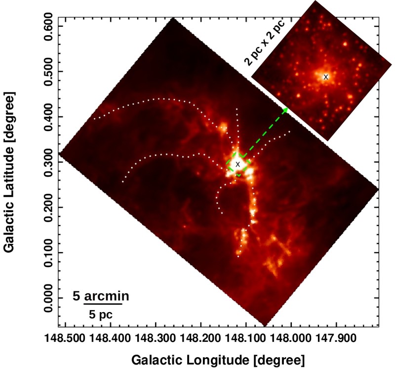
Figure 1: Central area of the G148.24+00.41 cloud as seen in $\it{Herschel}$ 250 $\mu$m band, showing the hub-filamentary morphology. The inset image shows the presence of an embedded cluster within the hub region (shown by a green box) at 3.6 $\mu$m. The filamentary structures are from Rawat et al. (2023). We note that for a better presentation of the molecular data, in this work, this figure, as well as the subsequent figures, are presented in the galactic coordinates, whereas figures of Rawat et al. (2023) are in the FK5 system.

2 Data

The molecular line observations of the G148.24+00.41 complex in ¹²CO, ¹³CO, and C¹⁸O lines (J = 1–0 transitions) at 115.271, 110.201, and 109.782 GHz, respectively, were observed with the 13.7-m radio telescope as part of the Milky Way Imaging Scroll Painting (MWISP; Su et al., 2019) survey, led by the Purple Mountain Observatory (PMO). The MWISP survey mapping covers the Galactic longitude from l = $9\degree.75$ to $230\degree.25$ and the Galactic latitude from b = $-5\degree.25$ to $5\degree.25$. The three CO isotopologue line observations were done simultaneously using a 3 $\times$ 3 beam sideband-separating Superconducting Spectroscopic Array Receiver (SSAR) system (Shan et al., 2012) and using the position-switch on-the-fly mode, scanning the region at a rate of 50″per second. The calibration was done using the standard chopping wheel method that allows switching between the sky and an ambient temperature load. The calibrated data were then re-gridded to 30″pixels and mosaicked to a FITS cube using the GILDAS software package (Guilloteau & Lucas, 2000). The antenna temperature ($T_{\mathrm{A}}$) has been converted to the main-beam temperature ($T_{\mathrm{{MB}}}$) using the relation $T_{\mathrm{{MB}}}=T_{\mathrm{A}}/B_{\mathrm{{eff}}}$, where B_eff is the beam efficiency, which is 46% at 115 GHz and 49% at 110 GHz. The spatial resolutions (Half Power Beam Width; HPBW) of the observations are around $\sim$ 49″, 52″, and 52″for ¹²CO, ¹³CO, and C¹⁸O , respectively, which correspond to a spatial resolution of $\sim$ 0.8$-$0.9 pc at the distance of the cloud ($\sim$ 3.4 kpc). The spectral resolution of ¹²CO is $\sim$ 0.16 km s^-1 with a typical rms noise level of the spectral channel is about 0.5 K, and of ¹³CO and C¹⁸O is $\sim$ 0.17 km s^-1 with a rms noise level of 0.3 K (for details, see Su et al., 2019).

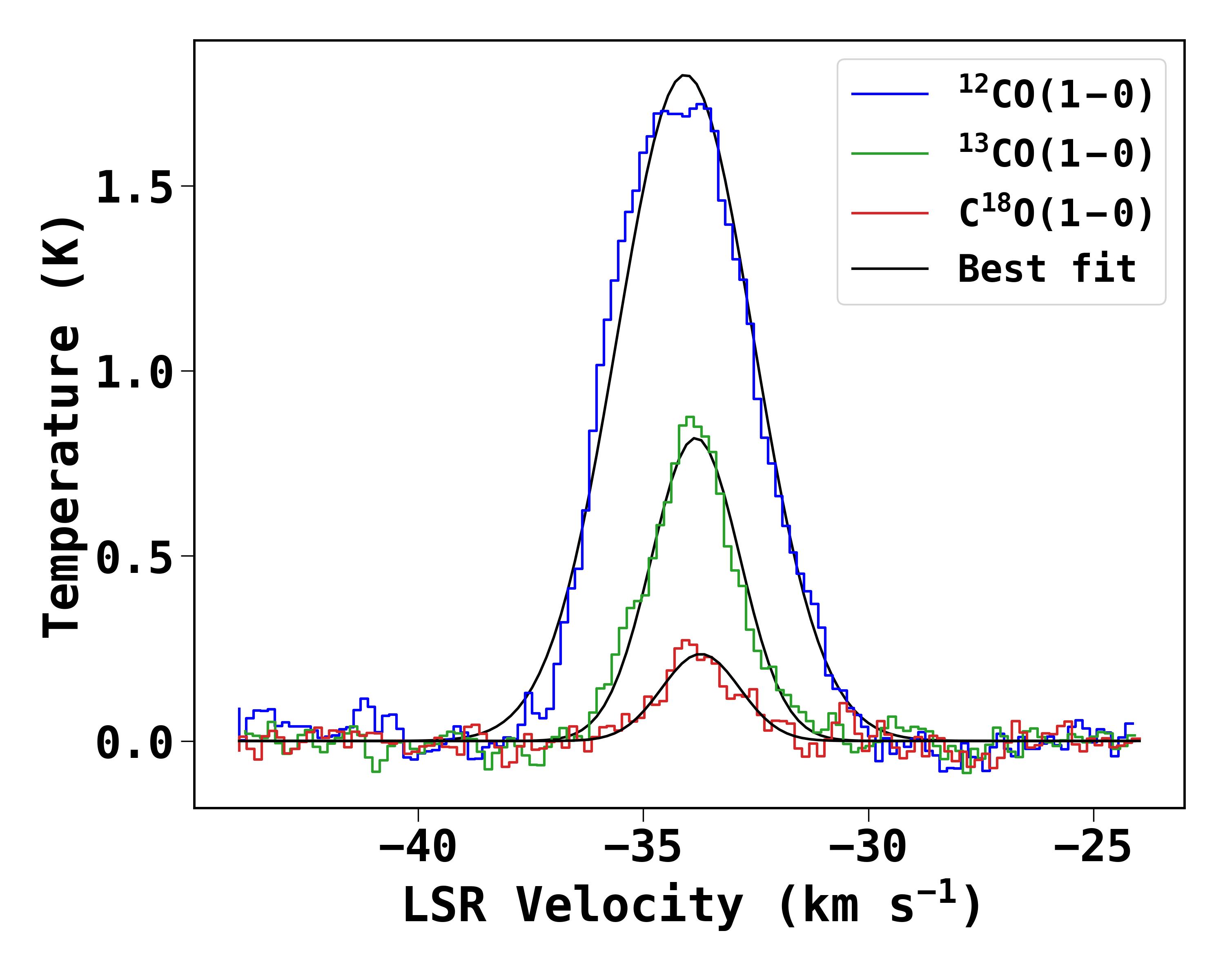
Figure 2: The average ¹²CO, ¹³CO, and C¹⁸O spectral profiles towards the direction of the G148.24+00.41 cloud. The black solid curve shows the Gaussian fit over the spectra.

3 Results and Analysis

The advantage of using the CO (1–0) isotopologues is that one can use the ¹²CO emission to trace the enveloping layer (i.e. $\sim$ 10² cm^-3) of the molecular cloud to reveal its large-scale low surface brightness structures and dynamics. On the other hand, the optically thin ¹³CO and C¹⁸O emission (discussed in Section 3.1.2) can trace the denser regions (i.e. $\sim$ 10³–10⁴ cm^-3) such as large-scale filamentary structure and dense clumps within the cloud. By combining the CO isotopologues, the overall properties of the diffuse regions of the cloud, as well as the gas properties and physical conditions of the dense structures within it, can be determined.

3.1 Global Cloud Morphology, Properties, and Kinematics

3.1.1 Gas morphology and kinematics

Rawat et al. (2023), based on ¹²CO  spectrum and comparing the CO gas morphology with the dust continuum images ($\it{Herschel}$ images at 250, 350 and 500  $\mu$m), showed that the G148.24+00.41 cloud component mainly lies in the velocity range of $-$37.0 km s^-1to $-$30.0 km s^-1 in agreement with the previous studies (e.g. Urquhart et al., 2008; Miville-Deschênes et al., 2017). Fig. 2 shows the average spectrum of all three isotopologues towards the cloud. We fitted a Gaussian function to the line profiles and derived the peak velocity, velocity dispersion ($\sigma_{1d}$), and velocity range of each spectrum, which are given in Table 1. The estimated line-width ($\Delta V=2.35\,\sigma_{1d}$) and 3D velocity dispersion ($\sigma_{3d}=\sqrt{3}\times\sigma_{1d}$) associated with the ¹²CO  profile are 3.55 and 2.62 km s^-1, for ¹³CO are 2.30 and 1.70 km s^-1, and for C¹⁸O are 2.04 and 1.51 km s^-1, respectively. We want to point out that the optical thickness of ¹²CO  may affect the velocity centroid and velocity dispersion of the line profile. Therefore, the ¹²CO data has been used to measure the global properties and distribution of low-density gas, while the kinematics of dense structures or properties of dense clumps have been derived using the ¹³CO  and C¹⁸O  data.

The integrated intensity (moment-0) maps of ¹²CO, ¹³CO, and C¹⁸O line emissions, integrated in the velocity range given in Table 1, are shown in Fig. 3. Also shown are the contours above 3$\sigma$ of the background value, where $\sigma$ is the standard deviation of the background emission. As discussed earlier, in molecular clouds, the ¹²CO, traces better the diffuse emission, while ¹³CO and C¹⁸O probe deeper into the cloud and trace higher column density regions. Though the spatial resolution of the data is relatively low, the presence of several filamentary structures can be seen in the ¹³CO map (details are discussed in section 3.2), while C¹⁸O emission seems better at tracing the central area and the dense clumpy structures of the cloud. In G148.24+00.41, we find that ¹³CO covers $\sim$ 87% of the ¹²CO emission, while C¹⁸O covers only 43%.

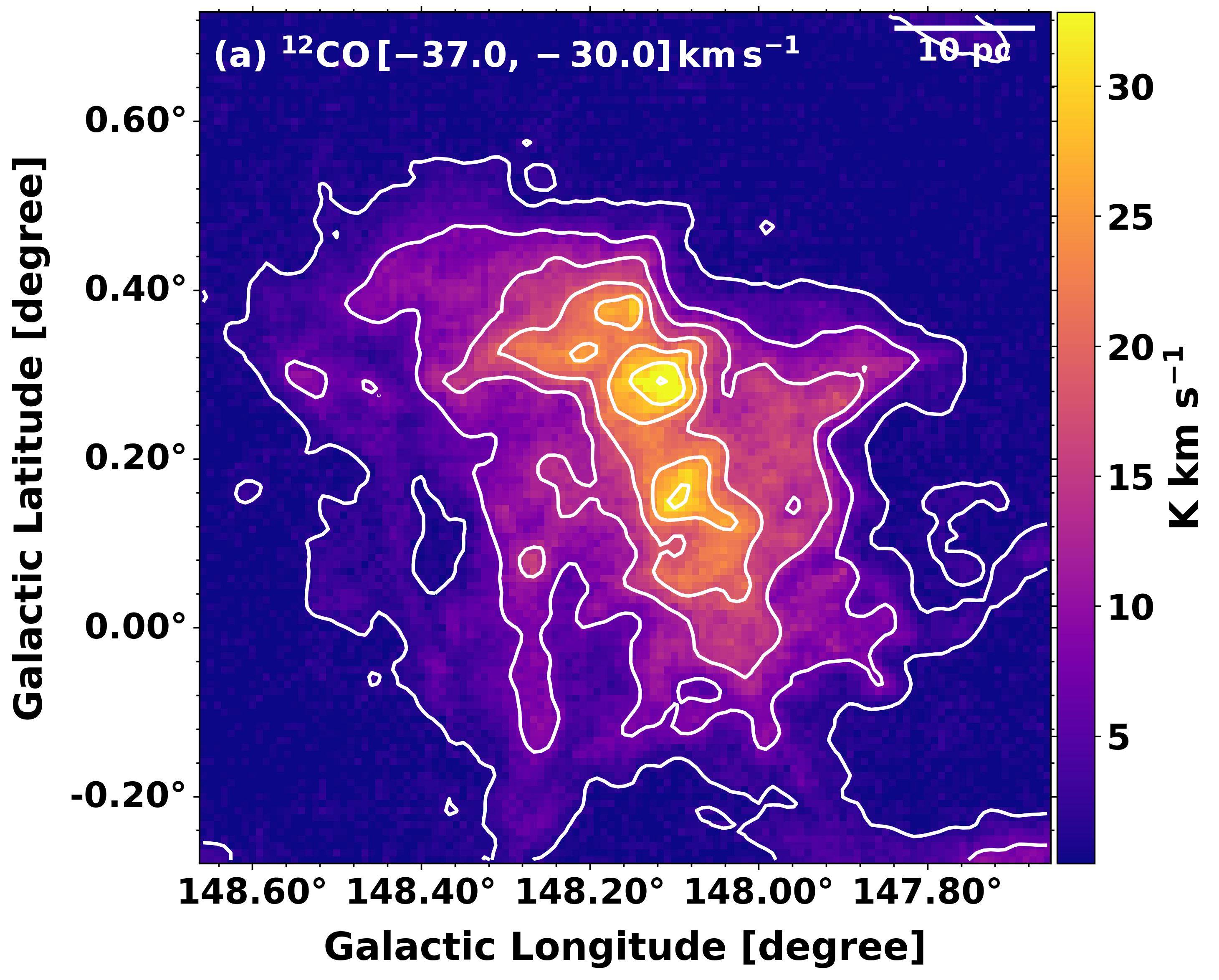
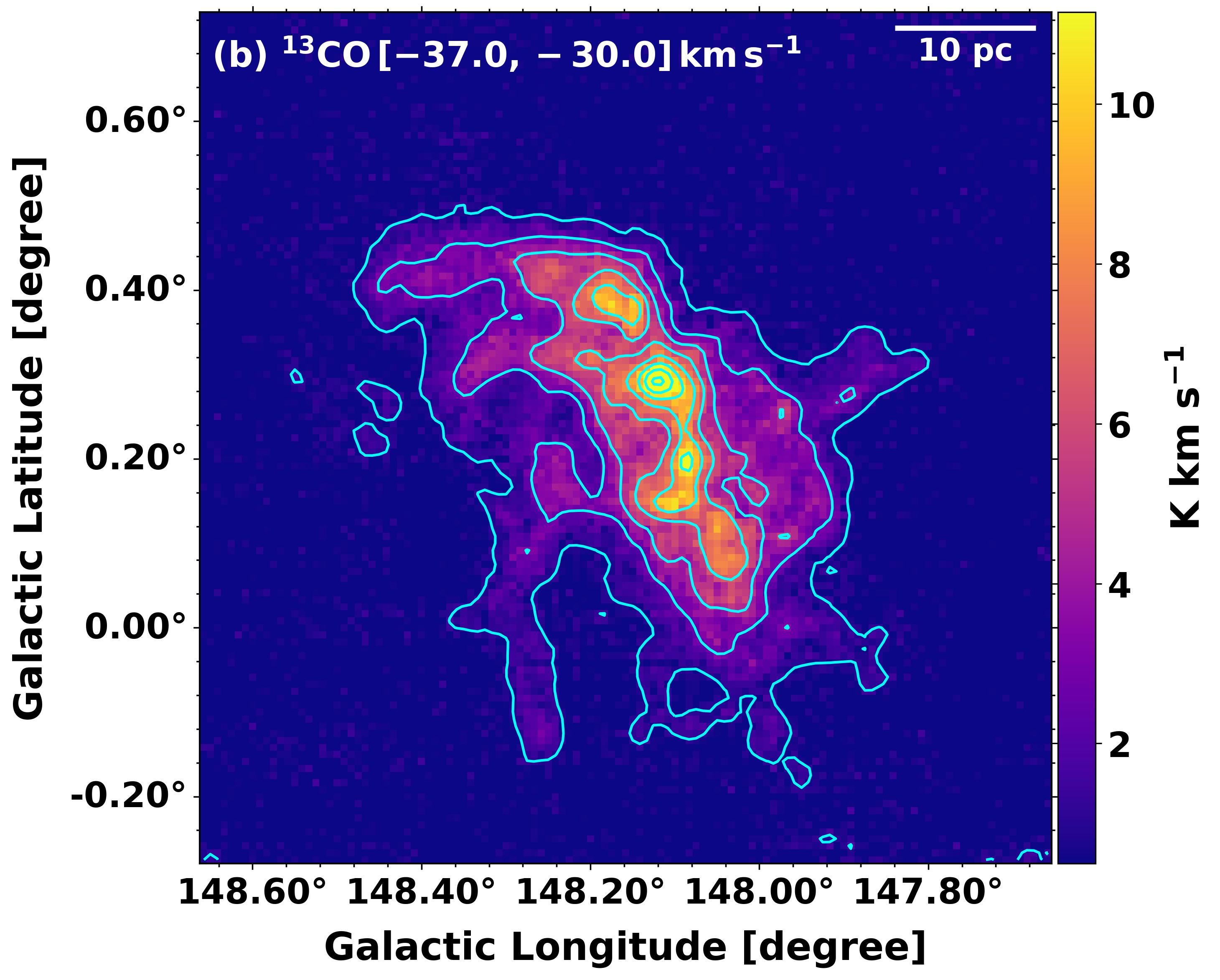
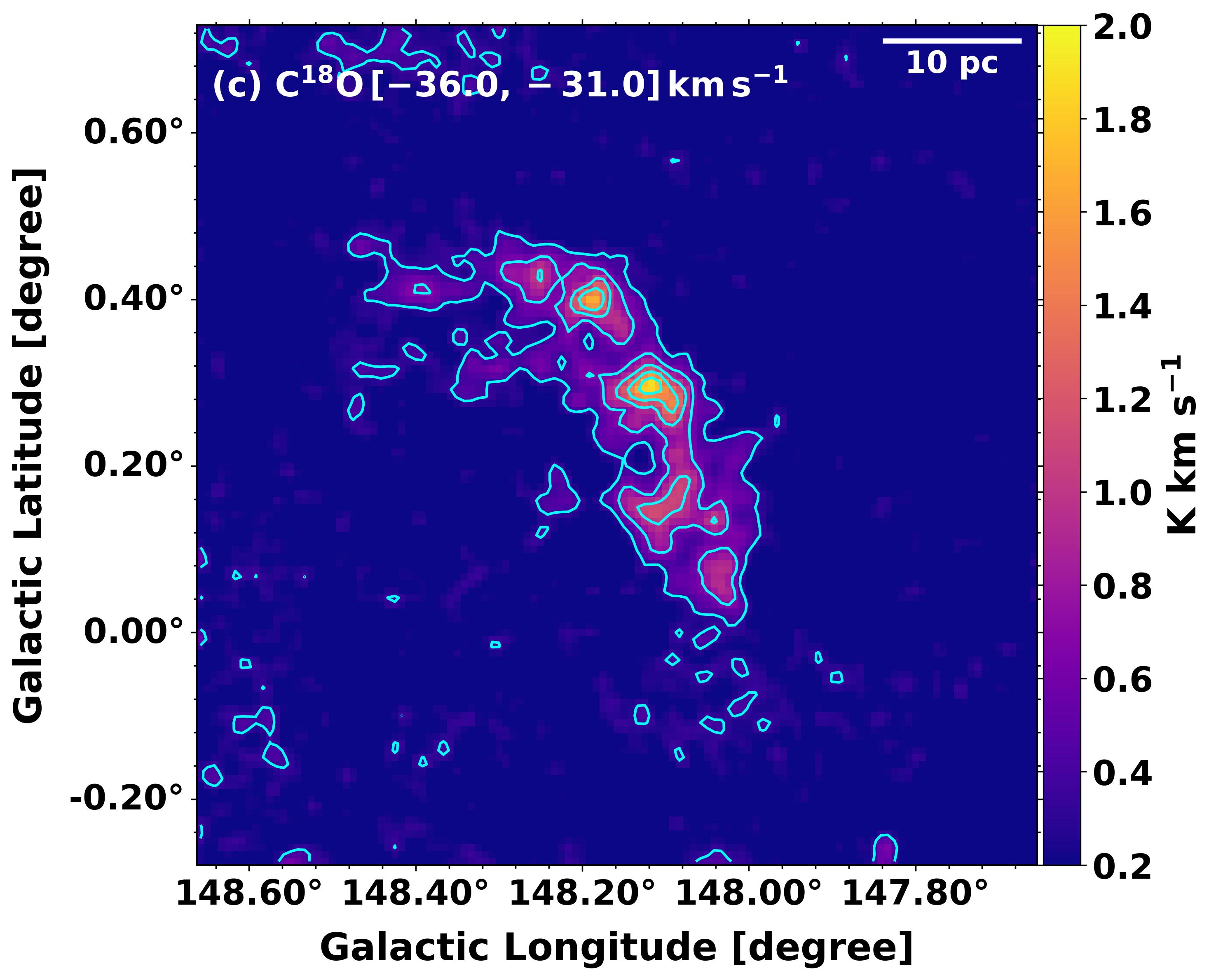
Figure 3: (a) ¹²CO  integrated intensity (moment-0) map of the cloud with contour levels at 1.5, 7.08, 12.67, 18.25, 23.83, 29.42, and 35 K km s^-1. (b) ¹³CO  integrated intensity map of the cloud with contour levels at 0.9, 2.7, 4.5, 6.3, 8.1, 9.9, 11.7, and 13.5 K km s^-1. (c) C¹⁸O  integrated intensity map of the cloud with contour levels at 0.35, 0.68, 1.01, 1.34, 1.67, and 2.0 K km s^-1. The contours are drawn 3$\sigma$ above the background value of individual maps. We note that the C¹⁸O map has been smoothened by 1 pixel to improve the signal.

In order to understand the overall velocity distribution and velocity dispersion of the ¹²CO and ¹³CO gas in the cloud, we made intensity-weighted mean velocity (moment-1) and velocity dispersion (moment-2) maps, which are shown in Figs. 4a-b and Figs. 4c-d, respectively. In general, the velocity distribution maps reveal that the outer extent of the cloud exhibits blue-shifted velocities relative to the systematic one, typically ranging from $-$36 to $-$34 km s^-1, while the central region displays a red-shifted velocity range, from $-$34 to $-$30 km s^-1. We note that, since moment analysis represents the mean velocity of the gas along the line of sight, it is insensitive to the kinematics of the multiple velocity structures, if present in the cloud (more discussion in Section 3.2.2). Figs. 4c-d shows that the velocity dispersion is not uniform across G148.24+00.41, it varies from 0.2 to 2.3 km s^-1, with a notable increase in the cloud’s central area. The velocity dispersion of ¹²CO gas may be on the higher side due to the optical depth effect, but this trend also holds true for the relatively optically thin ¹³CO line. In the central area, a patchy increase in velocity dispersion can be seen at several locations. We discuss more on this in Section 3.3.2. Additionally, the ¹²CO map reveals high velocity dispersion in the north-eastern side of the cloud, whose exact reason is not known to us. External shock compression can result in such high dispersions. Although a young ($\sim$ 4 Myr) H ii region is found to be present in the vicinity of the cloud (Romero & Cappa, 2009). However, the H ii region is located in the south-western direction of G148.24+00.41 and is also at a different distance (i.e. $\sim$ 1 kpc) with respect to it. A detailed investigation covering wider surroundings of G148.24+00.41 is needed to better understand its origin, which is beyond the scope of the present work.

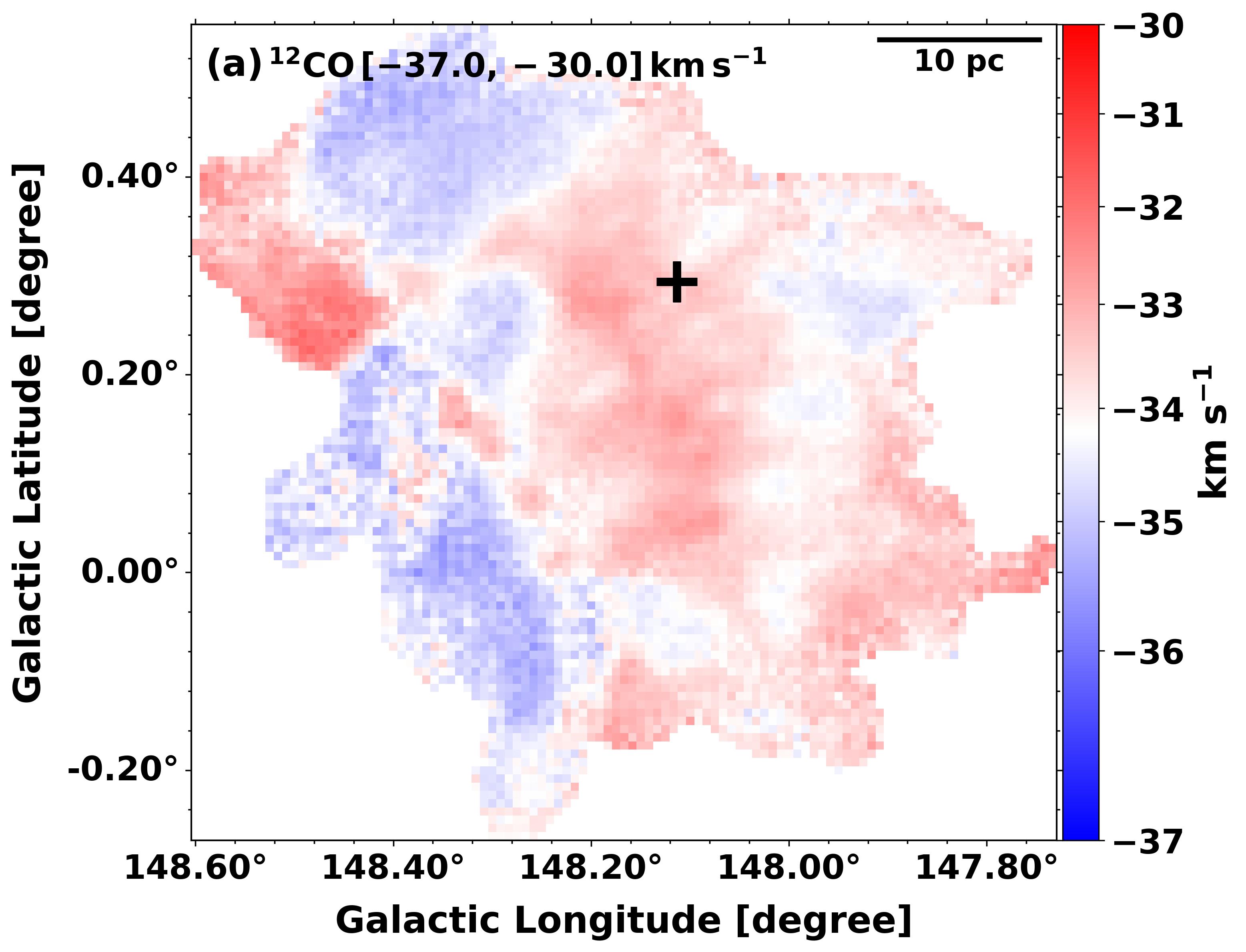
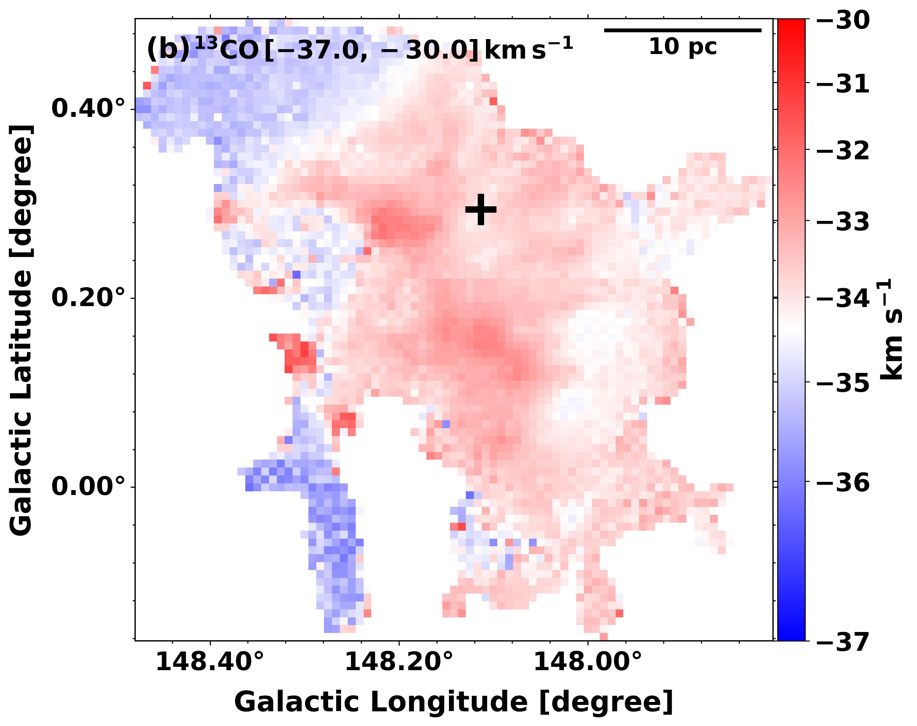
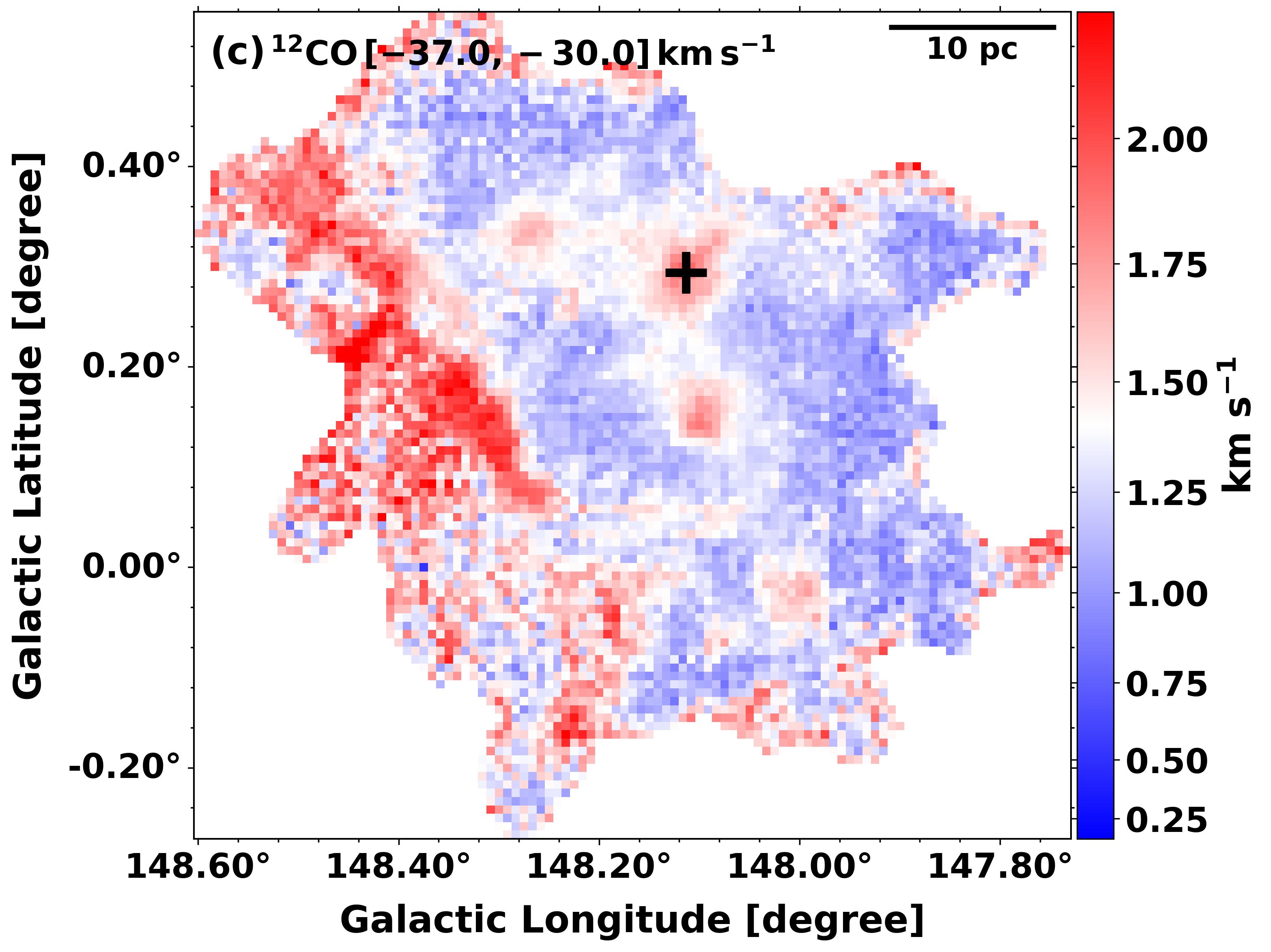
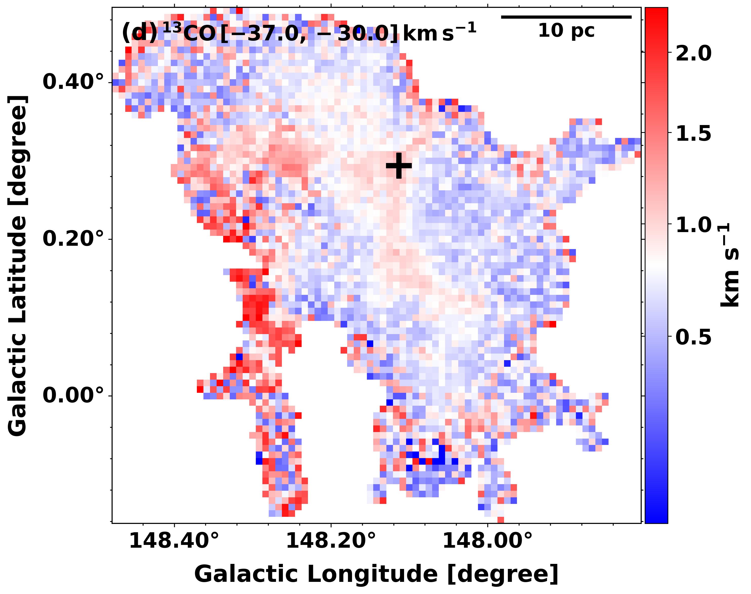
Figure 4: (a) ¹²CO and (b) ¹³CO velocity maps of G148.24+00.41. (c) ¹²CO and (d) ¹³CO velocity dispersion maps of G148.24+00.41. The location of the hub is marked with a plus sign.

3.1.2 Physical conditions and gas column density

Assuming the molecular cloud is under the local thermodynamic equilibrium (LTE) and ¹²CO is optically thick, the excitation temperature (T_ex), optical depth ($\tau$), and column density (N$(\mathrm{H}_{2})$) of the G148.24+00.41 cloud can be calculated with the measured brightness of CO isotopologues. Under LTE, the kinetic temperature of the gas is assumed to correspond to the excitation temperature.

The brightness temperature under the Rayleigh-Jeans approximation is expressed as $T_{\mathrm{{MB}}}$ = $f\times[J(T_{\mathrm{{ex}}})-J(T_{\mathrm{{bg}}})](1-e^{-\tau})$, where T_MB is the brightness temperature, $f$ is the beam filling factor, T_bg is the cosmic microwave background temperature, and $J(T)=\frac{h\nu}{k(\exp(h\nu/kT)-1)}$. Taking T_bg $\sim$ 2.7 K and assuming $f$=1, T_ex can be derived and written in a simplified form (Garden et al., 1991; Nishimura et al., 2015; Xu et al., 2018) as :

$$T^{1-0}_{\mathrm{{ex}}}=\frac{5.53}{\mathrm{ln}\left[1\ \ +\ \ \frac{5.53}{T^{12,1-0}_{\mathrm{{MB,peak}}}\ \ +\ \ 0.84}\right]},$$ (1)

where $T^{12,1-0}_{\mathrm{{MB,peak}}}$ is the peak brightness temperature of the ¹²CO emission along the line of sight. Based on the above formalism, we derived the excitation temperature at each pixel of the cloud. Fig. 5a shows the excitation temperature map, which ranges from 5 K to 21 K with a median around 8 K. The temperature map shows a relatively high temperature in the central region of the cloud with respect to the outer extent. This is likely due to the fact that the central region is heated by the protostellar radiation, where it has been found that protostars are actively forming (Rawat et al., 2023). The obtained average excitation temperature of the cloud is found to be similar to the ¹²CO based excitation temperature of massive GMCs with embedded filamentary dark clouds (e.g. $\sim$ 7.4 K, Hernandez & Tan, 2015, and references therein) and also similar to other nearby molecular clouds such as Taurus ($\sim$ 7.5 K, Goldsmith et al., 2008) and Perseus ($\sim$ 11 K, Pineda et al., 2008).

Next we derived the optical depth maps of ¹³CO and C¹⁸O gas using the following relations (Garden et al., 1991; Pineda et al., 2010):

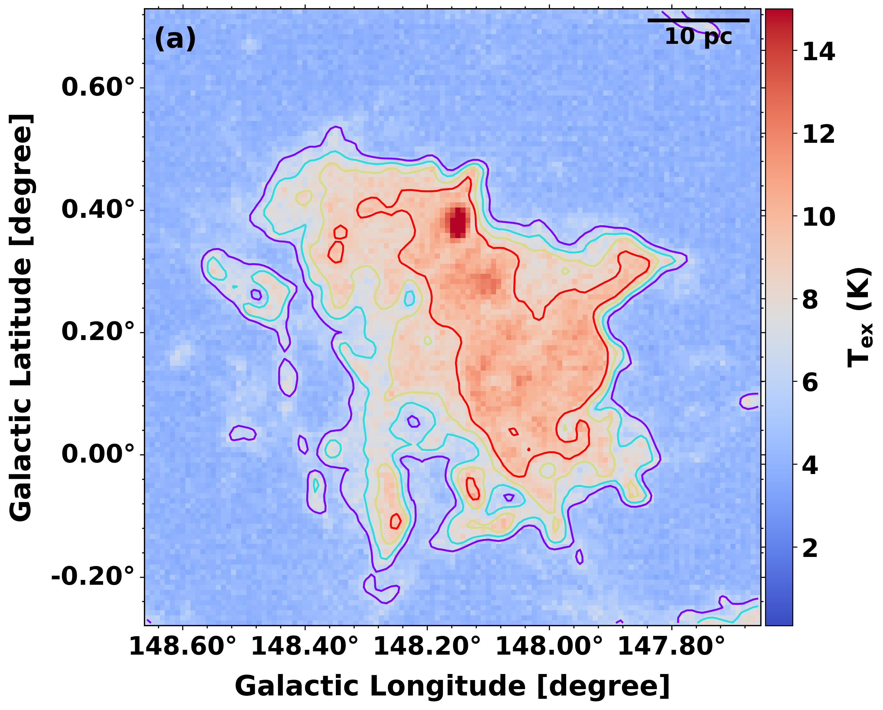
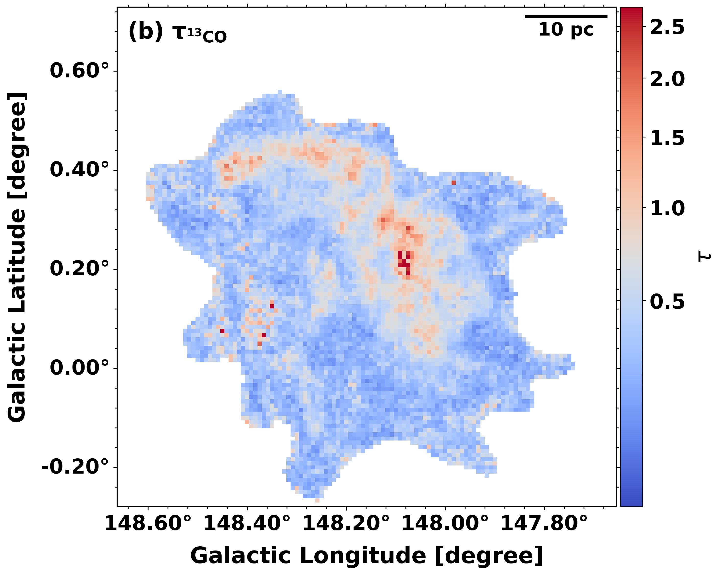
Figure 5: (a) Excitation temperature map overplotted with contours at 6, 7, 8, and 9 K. (b) Optical depth map of ¹³CO .

$$\tau_{13}=-\mathrm{ln}\left[1-\frac{T^{13}_{\mathrm{{MB,peak}}}}{5.29}\left[\frac{1}{\exp(5.29/T_{\mathrm{{ex}}})-1}-0.164\right]^{-1}\right]$$ (2)

$$\tau_{18}=-\mathrm{ln}\left[1-\frac{T^{18}_{\mathrm{{MB,peak}}}}{5.27}\left[\frac{1}{\exp(5.27/T_{\mathrm{{ex}}})-1}-0.166\right]^{-1}\right],$$ (3)

where $T^{13}_{\mathrm{{MB,peak}}}$ and $T^{18}_{\mathrm{{MB,peak}}}$ is the peak brightness temperature of ¹³CO and C¹⁸O , respectively.

The optical depths of ¹³CO and C¹⁸O lines are estimated to be 0.1 $<$ $\tau(\hbox{${}^{13}$CO}~{})$ $<$ 3.0 and 0.05 $<$ $\tau(\hbox{C${}^{18}$O}~{})$ $<$ 0.25, respectively. Fig. 5b shows the optical depth map of the ¹³CO emission. Within the cloud area, we found only a 5% fraction of the cloud area is of high ($\tau>1$) optical depth, implying that most of the observed ¹³CO emission is optically thin.

We then obtained the column density of ¹³CO and C¹⁸O using the following relations from Bourke et al. (1997):

$$N(\hbox{${}^{13}$CO}~{})_{\mathrm{{thin}}}=2.42\times 10^{14}\times\left(\frac{T_{\mathrm{{ex}}}+0.88}{1-\exp(-5.29/T_{\mathrm{{ex}}})}\right)\\ \times\frac{1}{J(T_{\mathrm{{ex}}})-J(T_{\mathrm{{bg}}})}\ \ \int T_{\mathrm{MB}}(\hbox{${}^{13}$CO}~{})dv$$ (4)

$$N(\hbox{C${}^{18}$O}~{})_{\mathrm{{thin}}}=2.42\times 10^{14}\times\left(\frac{T_{\mathrm{{ex}}}+0.88}{1-\exp(-5.27/T_{\mathrm{{ex}}})}\right)\\ \times\frac{1}{J(T_{\mathrm{{ex}}})-J(T_{\mathrm{{bg}}})}\ \ \int T_{\mathrm{MB}}(\hbox{C${}^{18}$O}~{})dv$$ (5)

However, the ¹³CO based column density may underestimate the column density in the central area of the cloud, where ¹³CO is optically thick. Many studies on the GMCs and Infrared Dark Clouds have accounted for line optical depth while estimating their physical properties (Roman-Duval et al., 2010; Hernandez et al., 2011). We, thus applied the following correction to the $N(\hbox{${}^{13}$CO})_{\rm{thin}}$ following Pineda et al. (2010); Li et al. (2015). Since the observed C¹⁸O emission is optically thin, no optical depth correction was made to $N(\hbox{C${}^{18}$O})_{\rm{thin}}$.

$$N(\hbox{${}^{13}$CO}~{})_{\mathrm{corrected}}=N(\hbox{${}^{13}$CO}~{})_{\mathrm{thin}}\times\frac{\tau_{13}}{1-e^{-\tau_{13}}}$$ (6)

We then convert the ¹³CO and C¹⁸O column density to the molecular hydrogen column density (N$(\mathrm{H}_{2})$) using the relation, N(H₂) = 7 $\times$ 10⁵ N(¹³CO) (Frerking et al., 1982) and N(H₂) = 7 $\times$ 10⁶ N(C¹⁸O) (Castets & Langer, 1995), respectively. The molecular hydrogen column densities from the ¹³CO and C¹⁸O gas emission are estimated to be around 0.9 $\times$ 10²¹ cm^-2 $<$ $\mathrm{N(H_{2})_{{}^{13}CO}}$ $<$ 2.4 $\times$ 10²² cm^-2 and 1.1 $\times$ 10²¹ cm^-2 $<$ $\mathrm{N(H_{2})_{C^{18}O}}$ $<$ 2.0 $\times$ 10²² cm^-2, respectively. We found for the common area, the column density of both the maps are in agreement with each other by a factor of 1.5. The observed variation in column density values might be due to the abundance variations of these isotopologues. For example, chemical models and observations suggest that selective photo-dissociation and fractionation can significantly affect the abundance of CO isotopologues (e.g. Shimajiri et al., 2015; Liszt, 2017).

Since ¹³CO covers a larger area and has a better signal-to-noise ratio compared to C¹⁸O , thus, we used ¹³CO based column density map for further analysis, such as in deriving the global properties of the cloud. Fig. 6 shows the ¹³CO based N$(\mathrm{H}_{2})$ map, tracing well the central dense location of the cloud. We find the peak value of N$(\mathrm{H}_{2})$ is around 2.4 $\times$ 10²² cm^-2, which corresponds to the location of the hub.

The ¹²CO emission in G148.24+00.41 is more extended than ¹³CO emission; thus, for estimating column density of the cloud area located outside the boundary of ¹³CO emission, we also estimated the hydrogen column density of each pixel directly from the ¹²CO intensity, I(¹²CO). To do so, we use the relation N(H₂) = X_CO I(¹²CO), where X_CO is the CO-to-H₂ conversion factor, whose typical value is $\sim$ 2.0 $\times$ 10²⁰ cm^-2 (K km s^-1)^-1 (Dame et al., 2001; Bolatto et al., 2013; Lewis et al., 2022) with an uncertainty of around 30% (Bolatto et al., 2013). We also estimated the total ¹²CO column density from the ¹³CO optical depth map, using an average value of ¹²CO / ¹³CO abundance of $\sim$ 60 (Frerking et al., 1982) and equation 3 of Garden et al. (1991). Doing so, we found that the total molecular hydrogen column density of the cloud based on both approaches is within a factor of 1.3.

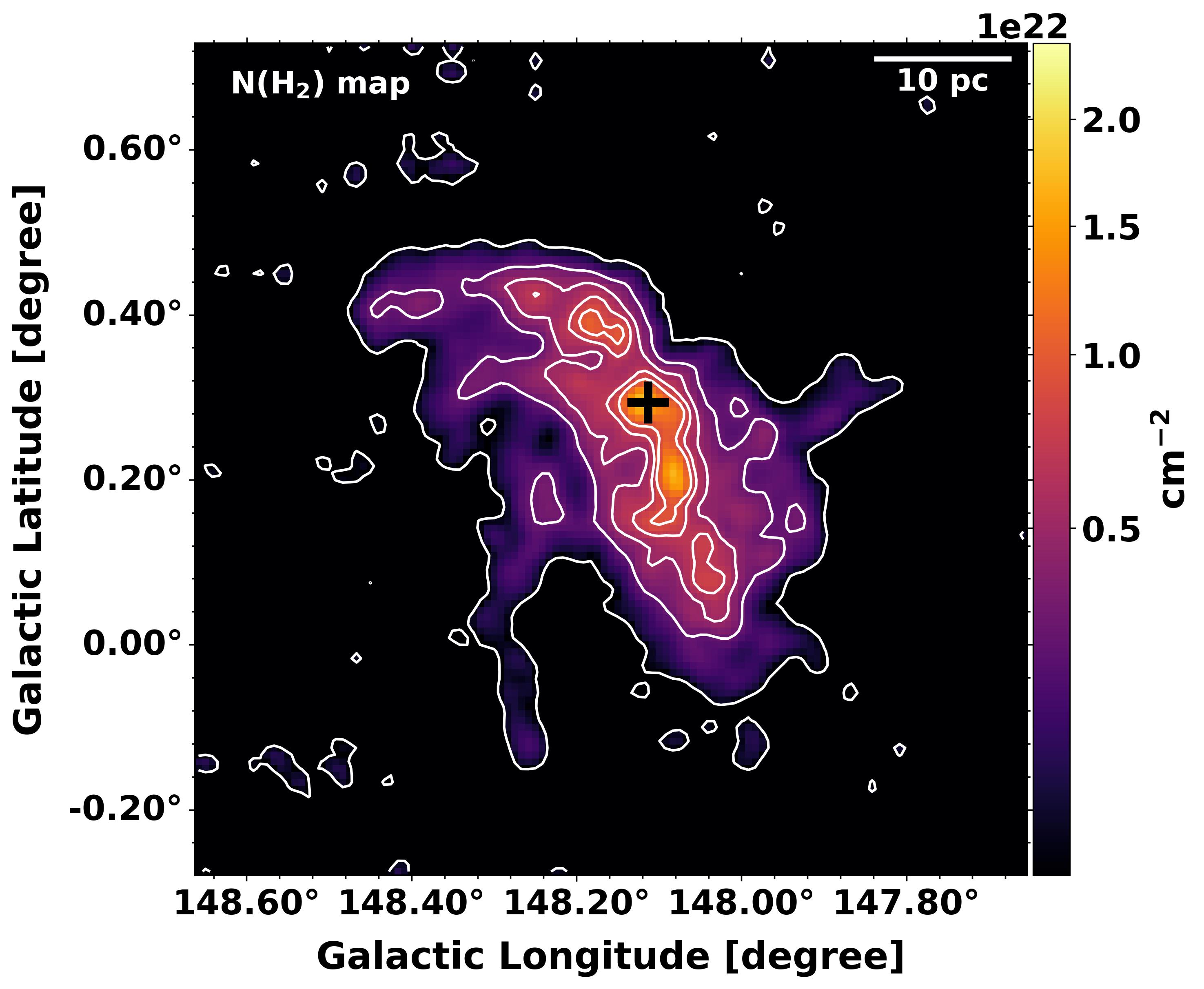
Figure 6: Molecular hydrogen column density map based on ¹³CO . The contour levels are shown above 3$\sigma$ of the background value, starting from 0.9 $\times$ 10²¹ to 9 $\times$ 10²¹ cm^-2 . The location of the hub is marked with a plus sign.

We then combined ¹²CO and ¹³CO column density maps to make a composite molecular hydrogen column density map. For the area lying outside the area of ¹³CO emission, we take the column density values from the ¹²CO emission. Although we use $\mathrm{N(H_{2})_{{}^{13}CO}}$ column density values within the ¹³CO emission area, we observed that some of the pixels in the central area of the ¹³CO map exhibit lower column density values than the neighbouring pixels. Overall, these outliers do not affect the measured global properties. Nonetheless, in these pixels, if the ratio (R) of $\mathrm{N(H_{2})_{{}^{13}CO}}$ to $\mathrm{N(H_{2})_{{}^{12}CO}}$ is found to be $>$ 1, the pixel values from the $\mathrm{N(H_{2})_{{}^{13}CO}}$ map are considered, otherwise, from the $\mathrm{N(H_{2})_{{}^{12}CO}}$ map. The combined composite map made in this way is shown in Fig. 7. The column density of the composite map lies in the range of 0.2 $\times$ 10²¹ cm^-2 to 2.4 $\times$ 10²² cm^-2. We checked the difference in column density values at the boundary of ¹³CO emission from both the tracers and found that they are within a factor of 1.2, thus reasonably agreeing with each other.

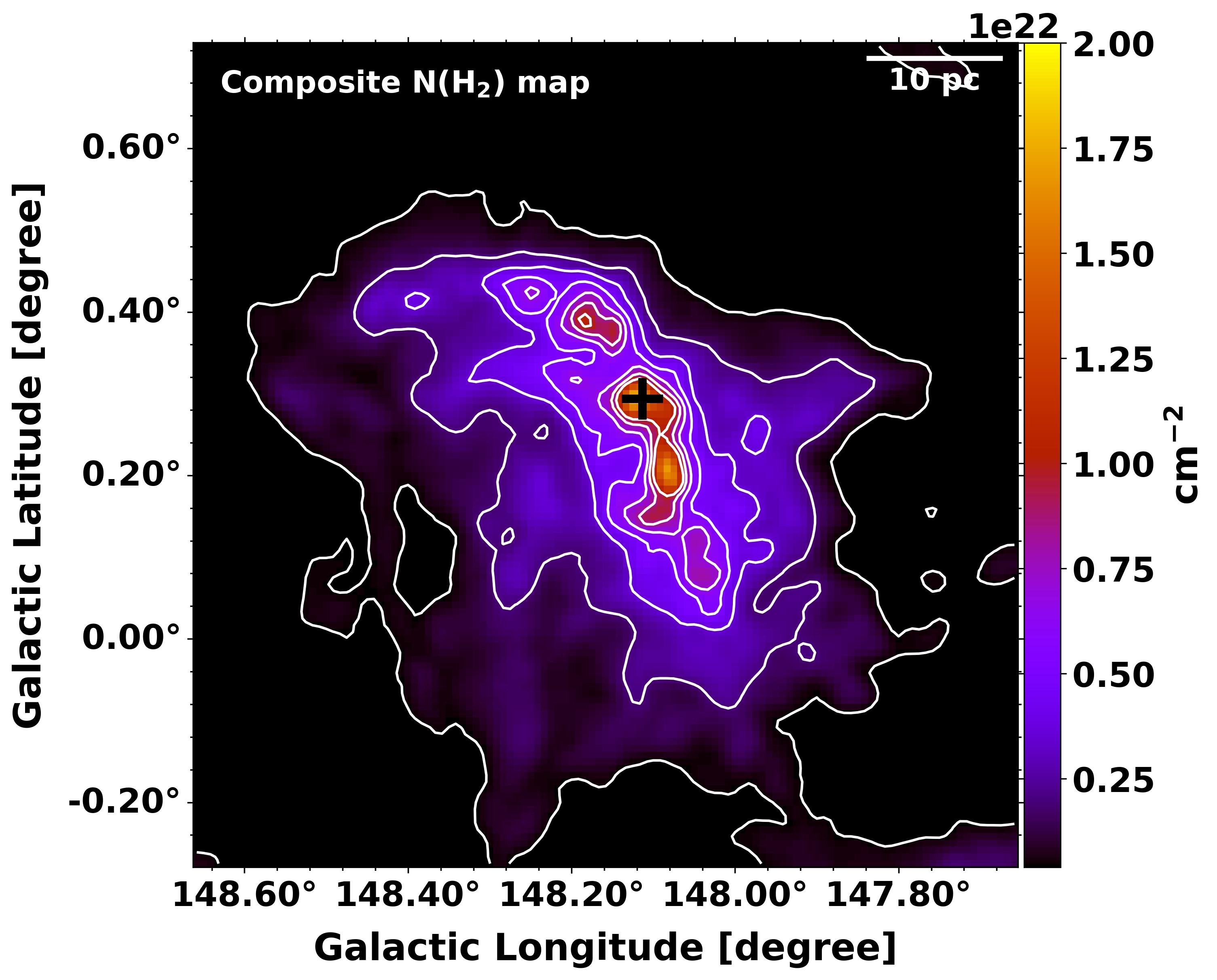
Figure 7: Composite N$(\mathrm{H}_{2})$ map based on ¹²CO  and ¹³CO column density maps. The contour levels are shown above 3$\sigma$ of the background value, starting from 4.3 $\times$ 10²⁰ to 1 $\times$ 10²² cm^-2 . The location of the hub is marked with a plus sign.

3.1.3 Global cloud properties and comparison with Galactic clouds

We obtained the cloud properties like mass, effective radius, surface density, and volume density, following the approach described in Rawat et al. (2023). Briefly, we estimated the mass of the cloud using the relation.

$$M_{\mathrm{c}}=\mu_{\mathrm{H_{2}}}m_{\mathrm{H}}A_{\mathrm{{pixel}}}\Sigma N(H_{2}),$$ (7)

where m_H is the mass of hydrogen, $A_{\mathrm{{pixel}}}$ is the area of a pixel in cm², and $\mu_{\mathrm{H_{2}}}$ is the mean molecular weight that is assumed to be 2.8 (Kauffmann et al., 2008). We define the outer extent (thus the area) of G148.24+00.41 for different tracers by considering emission within the 3$\sigma$ contours (see Fig. 3) and derive its properties within this area. The cloud mass from ¹²CO, ¹³CO, and C¹⁸O based N$(\mathrm{H}_{2})$ column density map, calculated above the 3$\sigma$ emission is $\sim$ 5.8 $\times$ 10⁴ M_⊙, $\sim$ 5.6 $\times$ 10⁴ M_⊙, and $\sim$ 3.5 $\times$ 10⁴ M_⊙, respectively. The cloud mass estimated from the composite column density map is found to be $\sim$ 7.2 $\times$ 10⁴ M_⊙. To check the boundness status of G148.24+00.41, we calculated its virial mass using the relation, $M_{vir}=126\times 1.33r_{\rm{eff}}\Delta V^{2}$, for density index, $\beta=1.5$ (see Eqn. 2 of Rawat et al., 2023). Using $r_{\rm{eff}}$ and $\Delta V$ values of ¹²CO, ¹³CO, and C¹⁸O  (see Table 1), the estimated $M_{\rm{vir}}$ is around $\sim$ 4 $\times$ 10⁴ M_⊙, 1.5 $\times$ 10⁴ M_⊙, and 8.6 $\times$ 10³ M_⊙, respectively. Since the virial mass of G148.24+00.41, as estimated by ¹²CO, ¹³CO, and C¹⁸O, is less than their respective gas mass, it implies that the cloud is bound in all three CO isotopologues. We acknowledge that the optical thickness of ¹²CO line can make the line profile broader, as discussed in Section 3.1.1, thus, the ¹²CO based virial mass can be an upper limit. Even then, the aforementioned boundness status of the cloud will remain true.

The typical uncertainty associated with the estimation of gas mass from the ¹²CO, ¹³CO, and C¹⁸O emissions is in the range 35$-$44%. Because the uncertainty in the assumed $\rm{X_{CO}}$ factor and in the isotopic abundance values of CO molecules, used in converting N(CO) to N$(\mathrm{H}_{2})$ is around 30 to 40% (Wilson & Rood, 1994; Savage et al., 2002; Bolatto et al., 2013). The distance uncertainty associated to the cloud is around 9%. In addition, the estimation of N(CO) is also affected by the uncertainty associated with the estimated gas kinematic temperature. In the present case, we find that the average gas kinetic temperature (8 K) is lower than the average dust temperature of the cloud, 14.5 $\pm$ 2 K (Rawat et al., 2023). When gas and dust are well mixed, the gas kinematic temperature better corresponds to the dust temperature, and this occurs when the density is $>$ 10⁴ cm^-3. For example, Goldsmith (2001) found that dust and gas are better coupled at volume densities above 10⁵ cm^-3, which are typically not traced by ¹²CO and ¹³CO data (n_crit < 10⁴ cm^-3). They find a temperature difference of $\sim$ 4 K at density $\sim$ 10⁵ cm^-3and completely negligible at density $\sim$ 10⁶ cm^-3. Moreover, it is also suggested that if the volume density of the gas is lower than the critical density of ¹²CO, this would lead to a lower excitation temperature (Heyer et al., 2009). Assuming the true average temperature of the gas is around 14 K, we estimated that it would change the ¹³CO column density by a factor of 14%, hence the estimated gas mass would also change by this factor.

In the present work, though we have derived the masses using canonical values of $\rm{X}$ factor and the CO abundances, however, it is worth mentioning that many studies have suggested that these values increase towards the outer galaxy (Nakanishi & Sofue, 2006; Pineda et al., 2013; Heyer & Dame, 2015; Patra et al., 2022). Since G148.24+00.41 is located in the outer galaxy (i.e. $\sim$ 11.2 kpc from the Galactic centre), the derived masses are likely underestimations. For example, we find that implementing $\rm{X_{CO}}$ value from the relation given in Nakanishi & Sofue (2006), would increase the total $\mathrm{N(H_{2})_{{}^{12}CO}}$ column density and thus, the mass by a factor of $\sim$ 2.

The total gas mass estimated for G148.24+00.41 in the present work using the composite column density map, within uncertainty, agrees with the dust-based gas mass $\sim$ ($1.1\pm 0.5)\times 10^{5}$ M_⊙, derived by Rawat et al. (2023). In Table 1, we have tabulated the cloud mass, mean column density, effective radius, surface density, and volume density of the cloud. The derived surface mass density from ¹²CO, ¹³CO, C¹⁸O, and composite map is $\sim$ 52, 59, 72, and 63 M_⊙ pc^-2, respectively. The surface mass density from ¹²CO is similar to the value which we have obtained for G148.24+00.41 from the dust continuum and dust extinction-based column density maps for the same area, (i.e. $\Sigma_{\rm{gas}}$ = 54 M_⊙ pc^-2, see Rawat et al., 2023). Since the isotopologues trace different areas of the cloud, their estimated surface densities are different, with a gradual increase from low-density to high-density tracer.

Comparing the properties of G148.24+00.41 with other Galactic clouds, we find that the ¹²CO surface density of G148.24+00.41 is significantly higher than the average surface density ($\sim$ 10 M_⊙ pc^-2) of the outer Galaxy molecular clouds of our own Milkyway (Miville-Deschênes et al., 2017). Miville-Deschênes et al. (2017) studied Galactic plane clouds using ¹²CO and found that the average mass surface density of clouds is higher in the inner Galaxy, with a mean value of 41.9 M_⊙ pc^-2, compared to 10.4 M_⊙ pc^-2 in the outer Galaxy. Similarly, we also find that the derived ¹³CO surface density of G148.24+00.41 is on the higher side of the surface densities of the Milkyway GMCs studied by Heyer et al. (2009). Heyer et al. (2009) found an average surface density value $\sim$ 42 M_⊙ pc^-2 using ¹³CO data, assuming LTE conditions and a constant H₂ to ¹³CO abundance, similar to the approach used in this work. Recently Lewis et al. (2022) investigated nearby star or star-cluster forming GMCs, including Orion-A, using ¹²CO emission and similar X_CO factor used in this work. Comparing the surface densities of these clouds, we find that the surface density of G148.24+00.41 is higher than most of their studied GMCs (average $\sim$ 37.3 $\pm$ 10 M_⊙ pc^-2) and comparable to the surface density of Orion-A (see Fig. 8 of Lewis et al., 2022). All the aforementioned comparisons support the inference drawn by Rawat et al. (2023) on G148.24+00.41 based on the dust continuum analysis, i.e. G148.24+00.41 is indeed a massive GMC like Orion-A.

Table 1: G148.24+00.41 properties from CO emission. The mass of the cloud from $\rm{{}^{12}CO}$, $\rm{{}^{13}CO}$, and $\rm{C^{18}O}$ is calculated above 3$\sigma$ from the mean background emission. The FWHM is the line-width of the spectra, calculated as $\Delta V=2.35\sigma_{1D}$.

Emission	Velocity interval	Vpeak	FWHM ($\Delta V$)	Mean N$(\mathrm{H}_{2})$	Mass	n(H2)	reff	$\Sigma_{\mathrm{gas}}$
	(km s-1)	(km s-1)	(km s-1)	($\times$ 1021 cm-2 )	(M⊙)	(cm-3)	(pc)	(M⊙ pc-2)
12CO	($-$37.0, $-$30.0)	$-$34.07	3.55	2.3	5.8 $\times$ 104	30	18.8	52
13CO	($-$37.0, $-$30.0)	$-$33.83	2.30	2.6	5.6 $\times$ 104	37	17.3	59
C18O	($-$36.0, $-$31.0)	$-$33.72	2.04	3.2	3.5 $\times$ 104	63	12.4	72
Composite-map	($-$37.0, $-$30.0)	—	—	2.8	7.2 $\times$ 104	37	19.0	63
(12CO & 13CO )

3.2 Filaments and Filamentary Structures

As mentioned in Section 1, based on dust continuum maps, Rawat et al. (2023) suggested that the central cloud region likely consists of six filaments, forming a hub filamentary system (HFS) with the hub being located at the nexus or junction of these filaments. Molecular clouds with HFSs are of particular interest because these are the sites where cluster formation would take place, as advocated in many simulations (e.g. Naranjo-Romero et al., 2012; Gómez & Vázquez-Semadeni, 2014; Gómez et al., 2018; Vázquez-Semadeni et al., 2019). Massive and elongated hub regions are sometimes referred to as “ridges” (e.g. Hennemann et al., 2012; Tigé et al., 2017; Motte et al., 2018).

The line-of-sight (LOS) velocity gradient, traced by molecular lines, is commonly interpreted as a proxy for the plane-of-sky (POS) gas motion. Recent molecular line observations have revealed the kinematic structures of several HFSs in nearby clouds, and significant velocity gradients are observed along several filaments that are attached to HFSs (e.g. Liu et al., 2012; Friesen et al., 2013; Hacar et al., 2018; Dewangan et al., 2020; Chen et al., 2020; Yang et al., 2023; Liu et al., 2023). These gas motions are thought to represent dynamical gas flows which are fuelling the hub. In the following, we identify and characterize the filamentary structures in the cloud and discuss their role in star and cluster formation observed in the cloud.

3.2.1 Identification of global filamentary structures

We used a python-based package - $\it{FilFinder}$ (Koch & Rosolowsky, 2015) to identify the filamentary structures of the cloud (details of FilFinder is given in Appendix A) using the ¹³CO based molecular hydrogen column density map. Fig. 8 shows the extracted skeletons of the G148.24+00.41 cloud. It can be seen that the $\it{Filfinder}$ algorithm reveals several filamentary structures, including the main central filament that runs from north-east to south-west, and also several nodes where the filaments are intersecting.

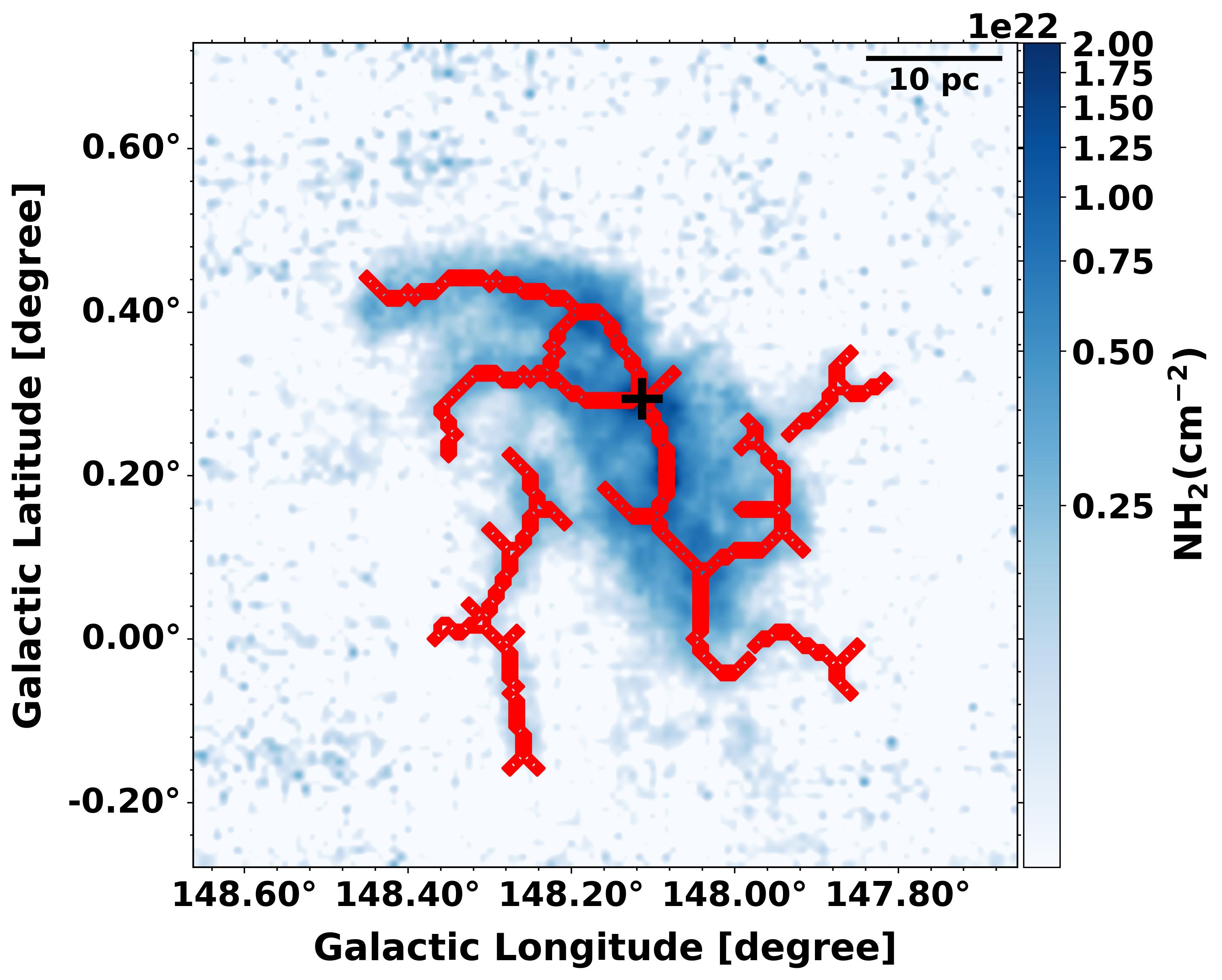
Figure 8: Global skeletons of G148.24+00.41 showing the filamentary structures, main ridge, nodes, and central hub location, over the ¹³CO based N$(\mathrm{H}_{2})$ map. The location of the hub is marked with a plus sign.

The column density map is created from the integrated intensity map. So it’s important to acknowledge that in the integrated intensity map, multiple individual velocity features may blend together and appear as a single one, as observed in nearby filamentary clouds (e.g. Hacar et al., 2013, 2017) or in distant ridge (e.g. Hu et al., 2021; Cao et al., 2022). Velocity sub-structures of gas in a cloud can be inspected using channel maps, in which the emission integrated over a narrow velocity range is examined. It is then possible to identify individual velocity coherent structures that are very likely to correspond to the physically distinct structures of the cloud.

3.2.2 Small-scale gas motion and velocity coherent structures

Fig. 9 shows the ¹³CO velocity channel maps with a step of 0.34 km s^-1. As can be seen from the channel maps, along with several compact emissions, multiple spatially elongated velocity structures are also present. These elongated structures are marked as St-1, St-2, St-3, St-4, St-5, and St-6 on the map. The location of these structures in the map corresponds to either the maximum intensity feature or has relatively the longest distinct visible structure, or both. These structures have noticeable differences in velocity because they emerge in different velocity channels.

The majority of these structures appear to move towards the hub location, marked by a plus sign on the map. The merger and convergence of these structures form a nearly continuous structure in the central area of the cloud that we refer to as the "ridge" in which the hub is located. The ridge is marked by a solid green line on the channel map. The ridge also seems to be attached to several small-scale strand-like, nearly perpendicular elongated structures (shown by arrows in Fig. 9). The kinematic association of such perpendicular structures with the main filament/ridge indicates the possible direct role of the surrounding gas on the formation and growth of the main filament/ridge (e.g. Cox et al., 2016). Besides, one can see that the structure, St-2, is composed of 2-3 small-scale filamentary structures that are seen in the channel maps at around $-$35.1 to $-$ 34.4 km s^-1. These structures are indistinguishable in the integrated intensity map shown in Fig. 3b, emphasizing that some of the elongated filamentary structures that we are seeing in the integrated intensity map could be the sum of multiple velocity coherent structures.

3.2.3 Likely velocity coherent filaments

In molecular clouds, small-scale velocity coherent filaments (VCF) have been identified using position-position-velocity (PPV) maps, where the velocity components are grouped based on how closely they are linked in both position and velocity simultaneously (e.g. Hacar et al., 2013). In the literature, identification of VCFs is primarily done using high-resolution and high-density tracer (e.g. NH₃, N₂H⁺, C¹⁸O ) data cubes and preferentially on the nearby clouds, where structures are well resolved (e.g. Hacar et al., 2017, 2018; Shimajiri et al., 2019). However, as witnessed from the channel maps, the gas kinematics of the cloud is quite complicated with overlapping structures. Disentangling and identifying individual velocity coherent structures is challenging with the present data. None the less, to identify the likely VCF of G148.24+00.41, we followed an approach similar to that of the nearby molecular clouds. We visually inspected the ¹³CO data cube and identified the velocity coherent structures that are continuous in position as well as velocity in the data cube. We then made the integrated intensity map of the structure by integrating the emission in the velocity range that encompasses the majority of its emission. In this way, we identified six likely velocity coherent filamentary structures in G148.24+00.41.

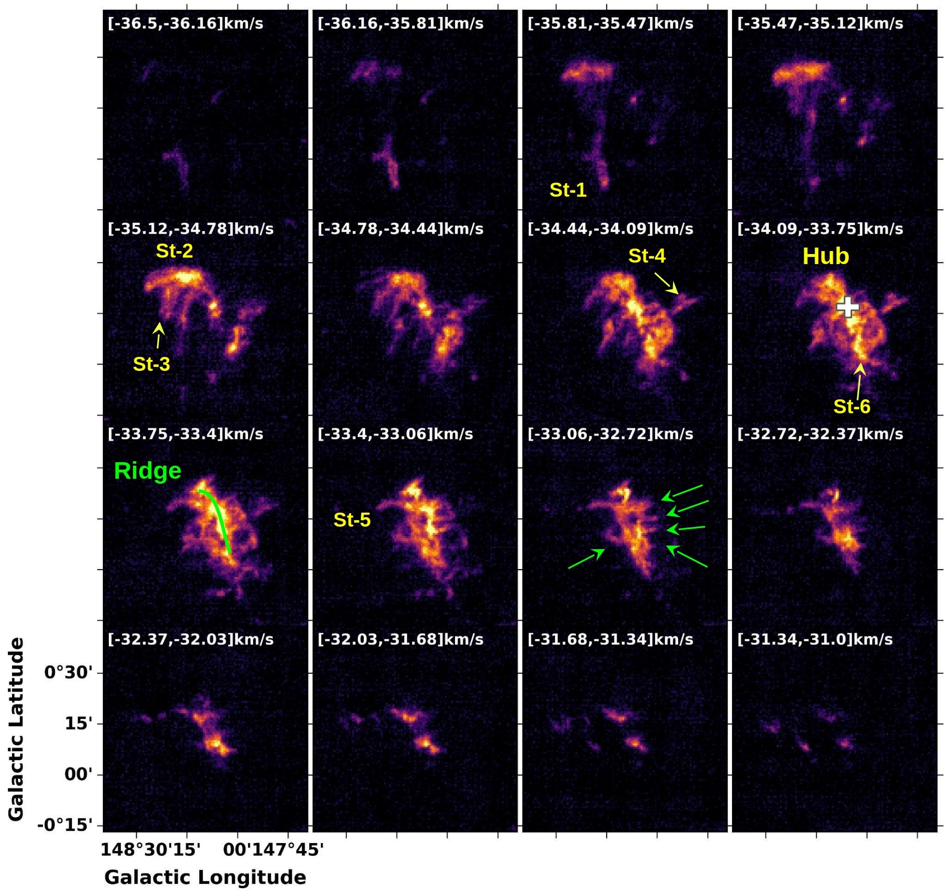
Figure 9: Velocity channel maps in units of K km s^-1for the ¹³CO emission. The velocity ranges of the channel maps are indicated at the top left of each panel. The ridge (green curve), strands (green arrows), structures (yellow arrows), and the hub location (plus) are marked in the channel maps.

Fig. 10 shows an example of an intensity map, integrated in the sub-velocity range, [$-$37.0, $-$34.0] km s^-1, where filament F1, F2, and F3 are identified, while F4, F5 and F6, are identified in the full velocity integrated intensity map (see Fig. 8). Compared to Fig. 10, the identification and delineation of F3 filament is confusing and difficult in Fig. 8, whereas in Fig. 10, the structure of F3 is better apparent, and seems to connect to F2. We note that although our approach is subject to the choice of velocity range, we find that except for one, the majority of the identified structures matched well with the structures shown in Fig. 8, but separated into different velocity coherent filaments.

All the identified structures are marked in Fig. 11 as F1, F2, F3, F4, F5, and F6. Most of these filaments correspond to the structures marked in Figure 9. The length of the filaments lies in the range of 15$-$40 pc. It is important to emphasize that while we have identified six probable filaments within the cloud based on our data, we acknowledge that the identification of such structures is also subject to the resolution of the data. Comparing the morphology of the ¹³CO integrated intensity based filamentary structures identified here with the dust-based filamentary structures visually identified by Rawat et al. (2023) in the central region of the cloud, we find that the filaments F2, F5, and F6 reasonably agree with the major filaments of Rawat et al. (2023) marked in Fig. 1. While the smaller $\it{Herschel}$ filaments attached to the hub are not identifiable in our low-resolution data. Future high-resolution observations may resolve the filaments into multiple sub-filaments (e.g. Hu et al., 2021). We proceed with the present available data to characterize the identified filamentary structures to get a sense of their role in the cluster formation of the cloud.

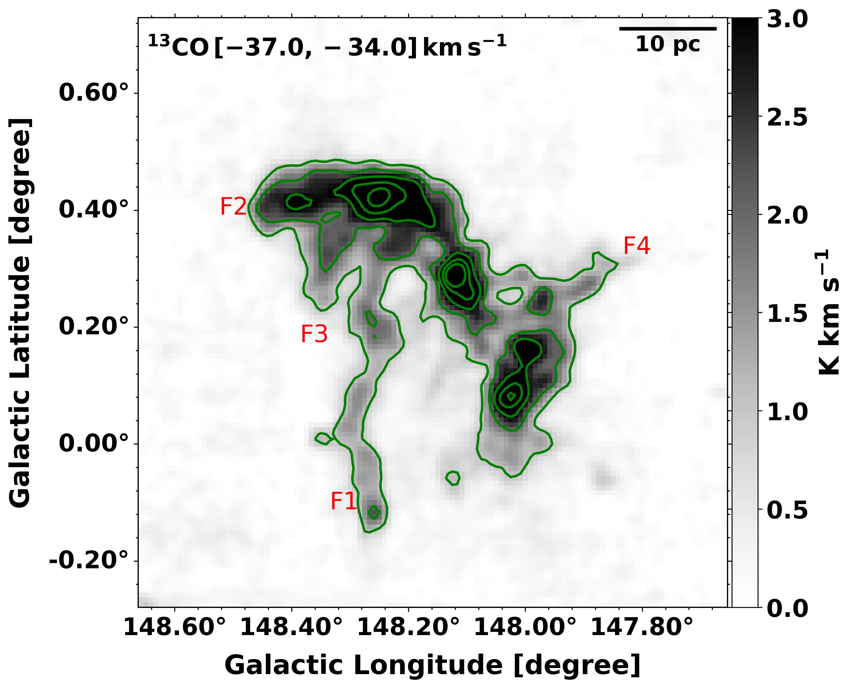
Figure 10: ¹³CO integrated intensity map in the sub-velocity range, $-$37.0 km s^-1to $-$34.0 km s^-1. The filamentary features- F1, F2, and F3 are prominent in this velocity range. Filament-F4 is also visible here.

3.2.4 Properties of the filaments

We make use of $\it{RadFil}$ (Zucker & Chen, 2018), a python-based tool to obtain the radial profile and width of the filament. $\it{RadFil}$ also uses the $\it{FilFinder}$ to generate the filament spines. It requires two inputs, image data, and filament mask, which we provided from the output of $\it{FilFinder}$ for the individual filament. Fig. 11 shows the extracted filament spines over their ¹³CO integrated intensity emission. $\it{RadFil}$ makes radial profiles of perpendicular cuts drawn along the filament spine as shown in Fig. 12a for filament F2 and then obtains filament width (Full Width Half Maxima, FWHM) by fitting a Gaussian function considering all the radial profiles (the detailed description of the procedures is given in Appendix B) as shown in Fig. 12b.

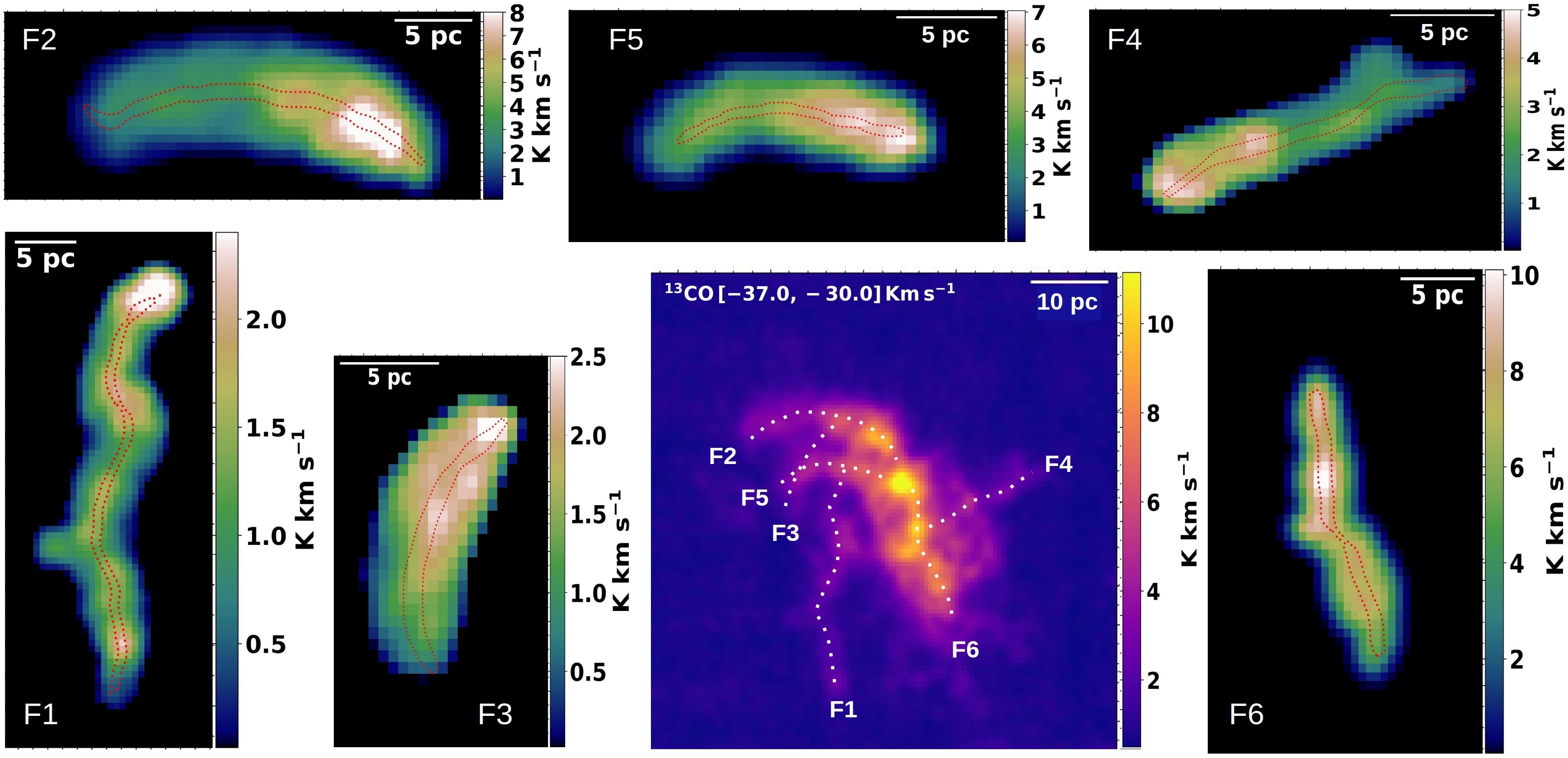
Figure 11: ¹³CO integrated intensity maps of individual filaments. The red-dotted curve in each filament map shows the filament spine extracted from $\it{Filfinder}$.

We obtained the deconvolved FWHM by taking into account the beam size (52″) as:
$\mathrm{FWHM_{decon}=\sqrt{FWHM^{2}-FWHM_{bm}^{2}}}$ (Könyves et al., 2015), where FWHM_bm is the beam size. The obtained FWHM_decon for all the filaments are listed in Table 2.

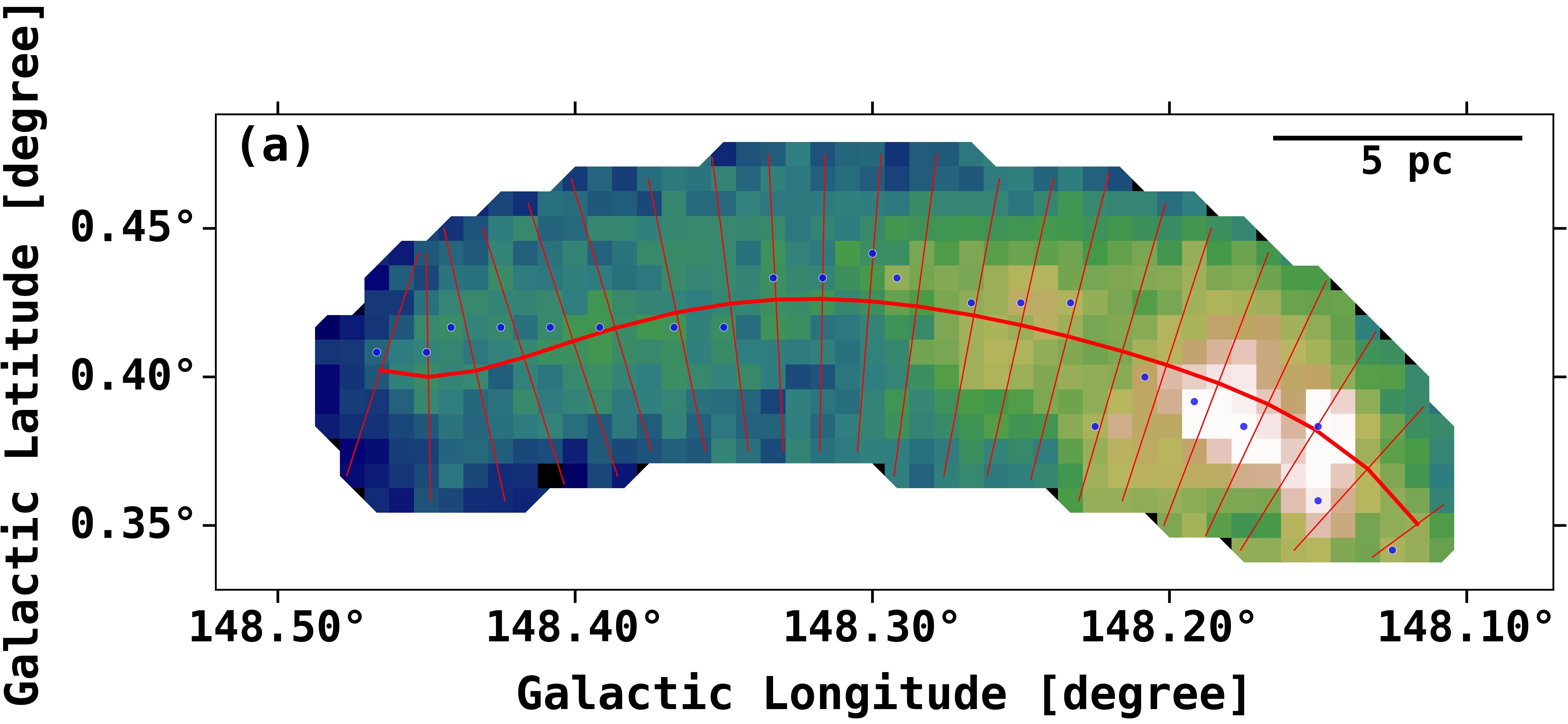
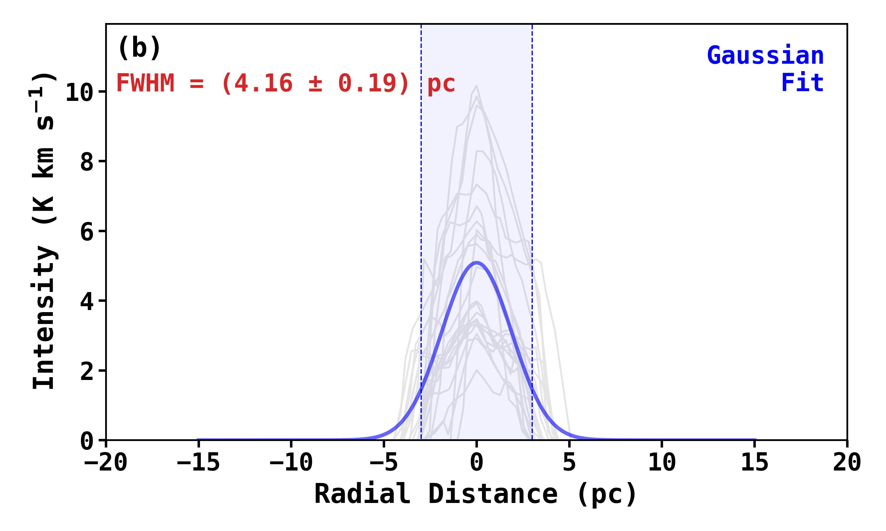
Figure 12: (a) The filament spine of F2 (red solid curve) shown over the ¹³CO integrated intensity emission, integrated in the velocity range, [$-$37.0, $-$34.0] km s^-1. (b) The radial profile of filament F2, built by sampling radial cuts (red solid lines perpendicular to filament spine shown in panel a) at every 2 pixels (roughly 1 beam size $\sim$ 52″or 0.9 pc). The radial distance at a given cut is the projected distance from the peak emission pixel, shown by blue dots in panel a. The grey dots trace the profile of each perpendicular cut, and the blue solid curve shows the Gaussian fit over these filament profiles. The light-blue shaded region shows the range of radial distance taken for the Gaussian fit.

In our case, the filament widths turn out to be in the range of 2.5$-$4.2 pc, with a mean $\sim$ 3.7 pc. The obtained widths are found to be higher than the typical width of $\sim$ 0.1 pc obtained from $\it{Herschel}$-based dust emission analysis of nearby clouds (e.g. André et al., 2010, 2014; Arzoumanian et al., 2019). However, it is worth noting that many observations and simulations have also argued that the width of filaments depends on many factors such as the fitted area, used tracer, resolution of the data, distance, evolutionary status of the filaments, and magnetic field (e.g. see Smith et al., 2014; Schisano et al., 2014; Federrath, 2016; Panopoulou et al., 2017; Suri et al., 2019; Panopoulou et al., 2022). For example, Panopoulou et al. (2022) found that the mean filament width for the nearby clouds is different from that of far away clouds. They also found that the mean per cloud filament width scales with the distance approximately as 4$-$5 times the beam size. Although the debate on the characteristic filament width of 0.1 pc is yet to be settled (see discussion in Panopoulou et al., 2017, 2022); we want to emphasize that our extracted filament widths might be on the higher side because G148.24+00.41 is located at a distance of $\sim$ 3.4 kpc and analysed with the low-resolution ($\sim$ 0.9 pc) and low-density tracer CO data. Moreover, some of the filaments (e.g. F2) could be the sum of a series of sub-filaments, whereas filaments in nearby clouds are well resolved. In addition, ¹³CO is tracing better the enveloping layer of the filaments. None the less, it is worth mentioning that using the PMO ¹³CO data, Liu et al. (2021) and Guo et al. (2022), found similar mean filament widths of $\sim$ 3.8 pc and $\sim$ 2.9 pc, respectively, for Galactic plane filamentary clouds located at 2.4 kpc and 4.5 kpc, respectively.

Future, high-resolution molecular data may be able to better characterize the filaments of G148.24+00.41. However, with the available data, we proceed to derive the properties of the filaments, such as mean line mass and column density, as well as the kinematics and dynamics of the filaments along their spines.

We estimated the total mass of the filaments within their widths using the same procedure discussed in Section 3.3.2, and then divide the mass by the length of the filaments to obtain mass per unit length, M_line, of the filaments. The properties of the filament, such as total mass, mean N$(\mathrm{H}_{2})$, aspect ratio (i.e. length/width), and M_line are tabulated in Table 2. The aspect ratios of the filaments are in the range of 4$-$10. Generally, a filament is characterized by an elongated structure with an aspect ratio greater than $\sim$ 3$-$5 (André et al., 2014). The M_line of the filaments F1, F2, F3, F4, F5, and F6 is found to be 92, 171, 93, 138, 233, and 396 M_⊙ pc^-1, respectively, with a mean around 187 M_⊙ pc^-1. M_line is a critical parameter for assessing the dynamical stability of the filaments, which we discuss in Section 4.1.

Table 2: Filament properties determined from ¹³CO . The filament F1, F2, and F3 are extracted in the velocity range, [$-$37.0, $-$34.0] km s^-1, while the filament F4, F5, and F6 are extracted in the velocity range, [$-$37.0, $-$30.0] km s^-1.

Filament	Length	Width	Mass	Massline	Masscrit	Mean N(H2)	$\mathrm{\frac{\sigma_{nt}}{c_{s}}}$
	(pc)	(pc)	($\times$ 103 M⊙)	(M⊙ pc-1)	(M⊙ pc-1)	($\times$ 1021 cm-2 )
F1	38.0	3.61	3.5	92	90	1.1	2.4
F2	25.7	4.16	4.4	171	94	3.0	2.4
F3	14.0	3.53	1.3	93	90	1.5	2.4
F4	18.1	3.28	2.5	138	215	2.3	3.7
F5	14.6	2.69	3.4	233	495	4.4	5.8
F6	17.4	2.49	6.9	396	283	9.0	4.0

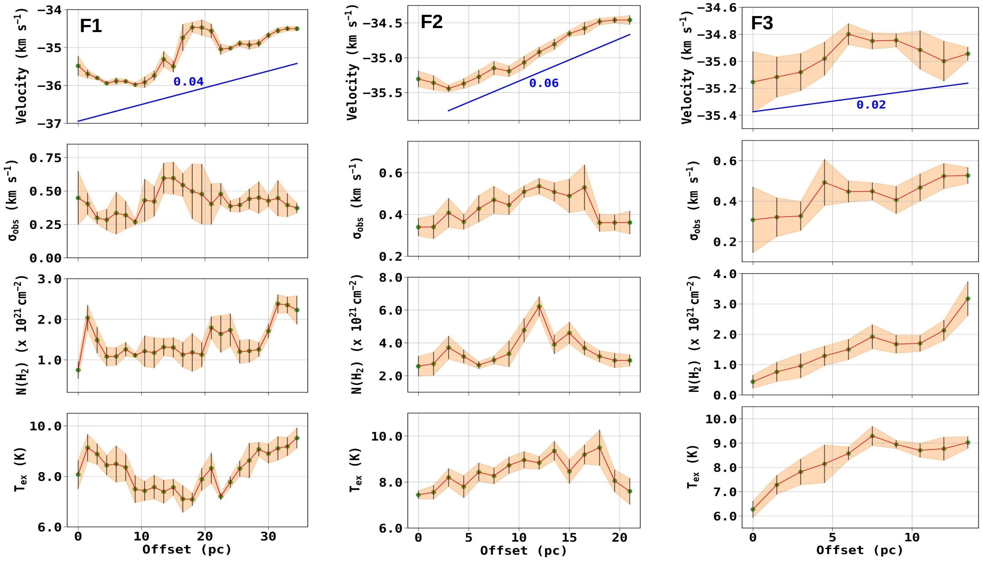
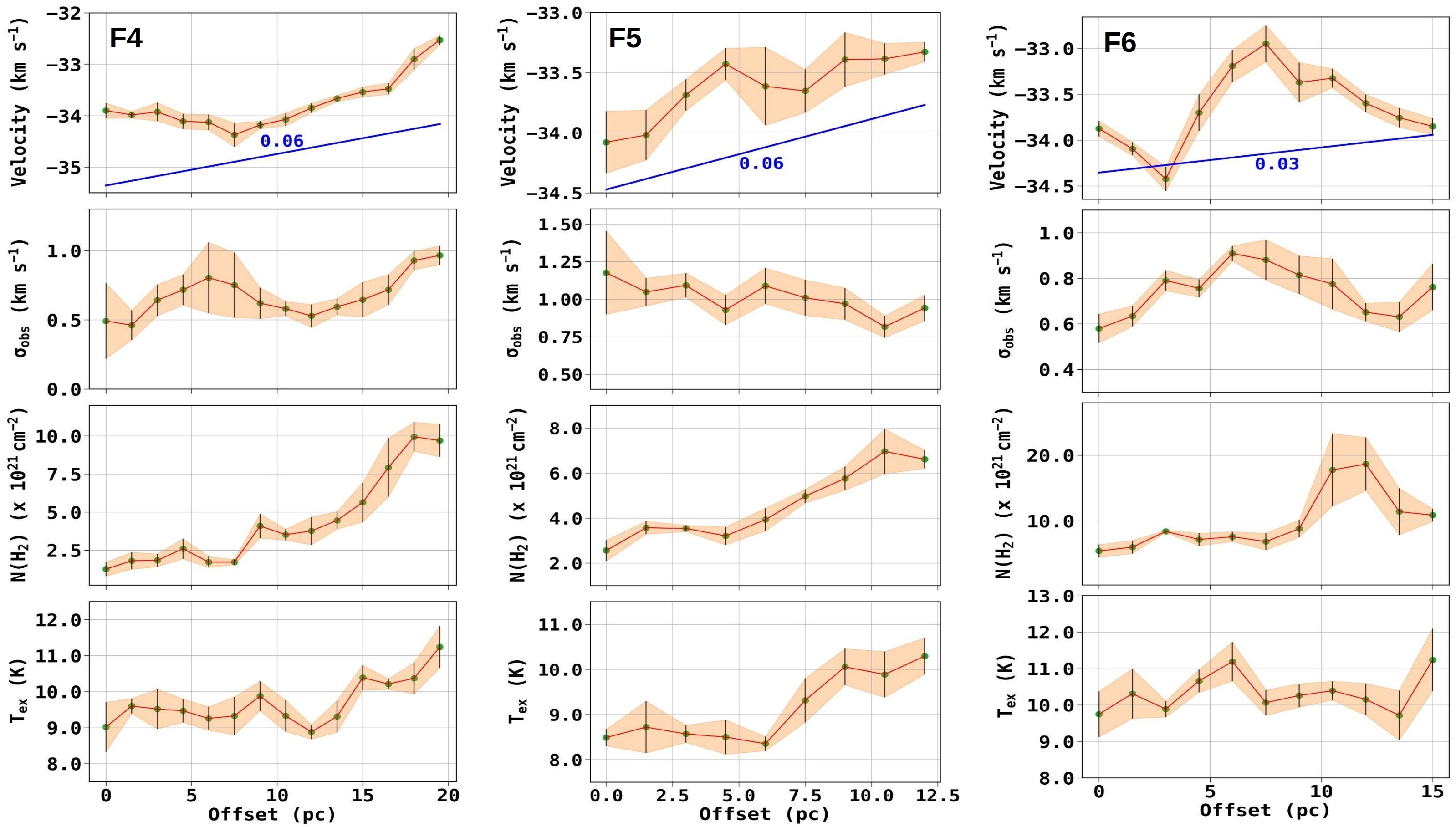
Figure 13: The average velocity, velocity dispersion, column density, and excitation temperature as a function of distance from the filament tail to the head, determined using ¹³CO . The offset 0 pc is at the filament tail. The error bars show the statistical standard deviation at each point. The blue solid line in the top panel of each filament plot shows the linear fit to the data points, whose slope (marked in the plot) gives the velocity gradient along the filament.

3.2.5 Kinematics and dynamics of the gas along the spine

To examine the kinematics, physical conditions, and dynamics of the gas along the filaments, we used ¹³CO molecular line data and estimated the parameters within the filament width. In Fig. 13, we show the variation of velocity, velocity dispersion, column density, and excitation temperature along the filament spines from their tail to head. We refer to the tail as the farthest point of the filament spine from the hub, while the head is referred to as the tip of the filaments near the hub.

In filamentary clouds, the observed velocity gradient along the long axis of the filaments is referred to as the longitudinal in-fall motion of the gas. To assess the amplitude of the longitudinal flow along the filaments’ long axis, we estimate the velocity gradient of each filament by doing the linear fit to the observed velocity profile along their spines. In some filaments (e.g. F6), noticeable fluctuations in the velocity profiles are seen. Similarly, for filaments F1 and F4, we see a negative gradient towards the tail of the filaments. This could be due to the local gravitational effect of the compact structures and associated star formation activity (e.g. Peretto et al., 2014; Yang et al., 2023). For example, in F1, a noticeable dense compact gas is seen in the tail (see Fig. 11), which might have reversed the flow of direction due to local gravity. Similar situations have also been seen in other filaments as well, for example, see Filament Fi-NW of the SDC 13 hub filamentary system (Peretto et al., 2014).

From the linear fit, the overall velocity gradient along the filament - F1, F2, F3, F4, F5, and F6 are found to be 0.04, 0.06, 0.02, 0.06, 0.06, and 0.03 km s^-1pc^-1, respectively. We note that the observed velocities are line-of-sight projected velocities, and thus, small velocity gradients in some filaments could be due to the filament orientation close to the plane-of-sky. Filaments with low inclination angles would make any identification of gas flows along the filaments very difficult. None the less, the observed velocity gradient for most of the filaments is close to the velocity gradient observed in large-scale giant molecular filaments (GMFs), i.e. filaments with lengths $>$ 10 pc. (e.g. Ragan et al., 2014; Wang et al., 2015; Zhang et al., 2019). For example, Ragan et al. (2014) found 0.06 km s^-1pc^-1, as an average of the 7 filaments in their sample. Similarly, Wang et al. (2015) find velocity gradient in the range 0.07$-$0.16 km s^-1pc^-1 in their sample of GMFs. Similar gradients have also been seen in some large-scale individual filaments (e.g. Hernandez & Tan, 2015; Zernickel, 2015; Wang et al., 2016). Higher velocity gradients have been observed in filaments at parsec and sub-parsec scales with high-resolution data, particularly in those filaments/elongated structures that are close to the hub or massive clumps (e.g. Liu et al., 2012; Chen et al., 2020; Zhou et al., 2022, 2023). The general finding is that the velocity differences ($\delta V$) between the filaments and central clump/hub become larger as they approach the central clump (i.e. $\delta V\propto\delta R^{-1}$, where $\delta R$ is the distance to the clump; e.g. see Hacar et al., 2022). This is also observed in G148.24+00.41 as in the proximity of hub (i.e. within the distance of 3 pc), we find that the associated filaments F2 and F6 show higher velocity gradients, $\sim$ 0.2 km s^-1pc^-1, towards their respective heads, which can be seen from Fig. 14. Fig. 14a shows the Position-Velocity (PV) diagram of the central filamentary area covering (see Fig. 8) spines of the filaments F2 and F6 (marked in Fig. 11). The figure also shows the positions of the clumps identified in Section 3.3. Fig 14b shows the gas velocity variation along the arrows marked in Fig. 14a. The gas profile shows a dip in the PV diagram, like the V-shaped structure found in other filaments, which is considered as a signature of gas inflow along the filaments towards a hub/clump (e.g. Zhou et al., 2022).

To understand the level of turbulence in the filaments, we also calculated the non-thermal velocity dispersion ($\sigma_{\rm{nt}}$) and Mach number ($M=\sigma_{\rm{nt}}/c_{\rm{s}}$) from the observed velocity dispersion. We calculate the non-thermal velocity dispersion ($\sigma_{\mathrm{nt}}$) from the total observed velocity dispersion ($\sigma_{\mathrm{obs}}$) using the relation,

$$\sigma_{\mathrm{nt}}=\sqrt{\sigma_{\mathrm{obs}}^{2}-\sigma_{\mathrm{th}}^{2}},$$ (8)

where $\sigma_{\mathrm{th}}$ = $\sqrt{k_{\mathrm{B}}T_{\mathrm{K}}/\mu_{\mathrm{i}}m_{\mathrm{H}}}$ is the thermal velocity dispersion. $T_{\mathrm{K}}$ is the gas kinetic temperature, $k_{\mathrm{B}}$ is the Boltzmann constant, and $\mu_{\mathrm{i}}$ is the mean molecular weight of the observed tracer (e.g. $\mu(\hbox{${}^{13}$CO}~{})=29$ & $\mu(\hbox{C${}^{18}$O}~{})=30$). The mean $\sigma_{\mathrm{obs}}$ is obtained from the velocity dispersion (moment-II) map within the filament region. Using the average $T_{\mathrm{ex}}$ of the filaments as $T_{\mathrm{kin}}$, we calculated the $\sigma_{\mathrm{th}}$ and $\sigma_{\mathrm{nt}}$ of the filaments. Using $\sigma_{\mathrm{nt}}$ and thermal sound speed, $c_{\mathrm{s}}$ = $\sqrt{k_{\mathrm{B}}T_{\mathrm{K}}/\mu m_{\mathrm{H}}}$ with mean molecular weight per free particle, $\mu$ = 2.37 (Kauffmann et al., 2008), we can also calculate the total effective velocity dispersion

$$\sigma_{\mathrm{eff}}=\sqrt{\sigma_{\mathrm{nt}}^{2}+c_{\mathrm{s}}^{2}},$$ (9)

The Mach number for the filaments is tabulated in Table 2. The gas in the individual molecular filaments of G148.24+00.41 is found to be supersonic with sonic Mach number $\sim$ 2$-$6. This is in agreement with the results of Wang et al. (2015) and Mattern et al. (2018) toward a sample of large-scale filaments measured with the low-resolution (30$-$46^′′) ¹³CO data using Galactic Ring Survey and SEDIGISM survey data (for details, see Table. 1 of Schuller et al., 2021). However, we want to stress that the derived properties are from the medium-density tracers such as ¹³CO , but the high-density tracers that would trace very central regions of the filament may give different results. For example, Pineda et al. (2010) comparing high-density and low-density tracers suggested that the sub-sonic turbulence is surrounded by supersonic turbulence in the filaments of the Perseus cloud. Results from high-resolution observations also show that the velocity dispersions of resolved nearby filaments and fibres are close to the sonic or sub-sonic speed (e.g. Hacar et al., 2013; Friesen et al., 2016; Hacar et al., 2017; Saha et al., 2022). All these results tend to suggest that the level of turbulence is scale-dependent, and subsonic velocity coherent filaments possibly condense out of the more turbulent ambient cloud/filament.

From Fig. 13, we also noticed that the majority of filaments exhibit an increasing velocity dispersion as they approach the hub or ridge. The figure also shows that in the majority of the filaments, the increase in velocity dispersion is proportional to the column density of the gas as we move from the tail to the head of the filaments, which is also evident in the integrated intensity maps shown in Fig. 11. In filaments, strong velocity gradients due to rotation have also been observed, but primarily at smaller scales, such as close to the dense clump or along the minor axis of the filaments. In the present case, the velocity gradients along the long-axis of the filaments over large scale ($>$ 5 pc), as well as the increase in velocity dispersion and column density as they approach the bottom of the potential well of the cloud, suggest for longitudinal flow of gas along the filaments toward the hub/ridge as found in numerical simulations (e.g. Heitsch et al., 2008; Carroll-Nellenback et al., 2014; Vázquez-Semadeni et al., 2019).

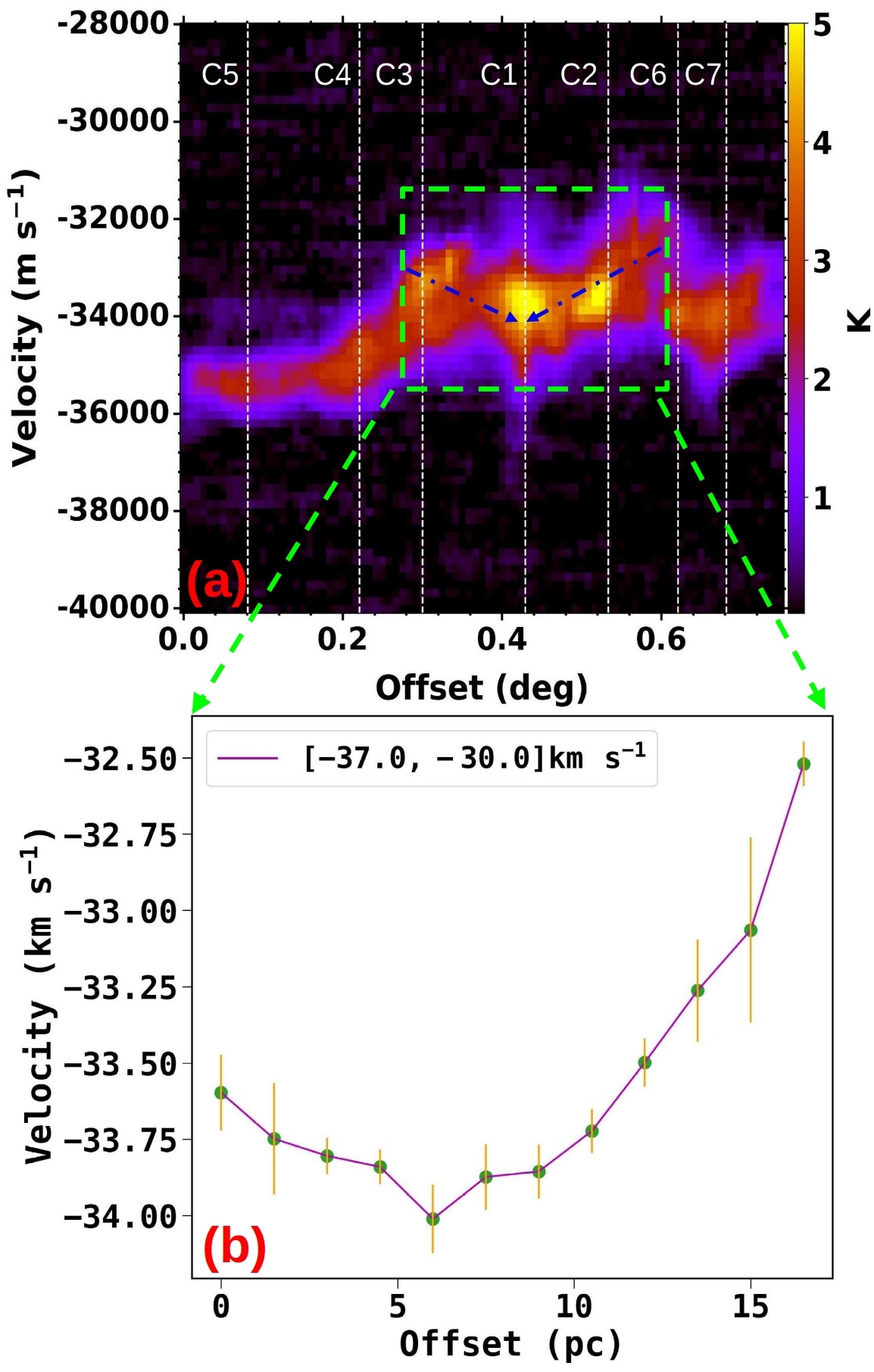
Figure 14: (a) The position-velocity (PV) diagram of the full ridge based on ¹³CO , which is shown in Fig. 9. The green-dashed box shows the region that is used to see the gas flow structure along the blue dashed-dotted arrows, toward the central hub/clump. The vertical dashed lines show the location of identified clumps, marked with their names (see Section 3.3). (b) The variation of average velocity with distance along the arrows (shown in panel a), which shows the velocity gradient towards the central hub/clump.

3.3 Dense Clumps and Properties

Fig. 3 suggests that the cloud has fragmented into several clumpy structures. These are the clumps of the cloud where star formation could take place. In order to understand the properties and dynamics of these clumps, we utilized C¹⁸O data, as it is a better tracer of denser gas and found to be optically thin in G148.24+00.41.

3.3.1 Identification of clumps

For identifying clumps of G148.24+00.41, we implemented the dendrogram (Rosolowsky et al., 2008) method using ASTRODENDRO python package. The dendrogram is a structure-finding algorithm that identifies hierarchical structures in the input two- or three-dimensional array. The output of the dendrogram depends on three parameters: the minimum value that defines the background threshold, the minimum delta or difference that defines the separation between two substructures, and the minimum pixels that defines the minimum number of pixels or size needed for the structure to be called an independent entity. We ran the dendrogram over the C¹⁸O integrated intensity map to find the clumps. We carefully investigate and set the following optimum extraction parameters to detect parsec scale clumpy structures while avoiding faint noisy structures. We set the minimum value to be 3$\sigma$ above the mean background emission, the minimum delta to be 1$\sigma$, and the minimum size to be 12 pixels. Doing so, we identified seven clumps in the cloud, which are marked in Fig. 15a as C1 to C7. The ID, size, and position angle of the clumps are tabulated in Table 3.

Table 3: Clump properties. The mass, line-width ($\Delta V=2.35\sigma_{\rm{obs}}$), virial parameter ($\alpha$), and the ratio of non-thermal velocity dispersion ($\sigma_{\rm{nt}}$) to thermal sound speed ($c_{\rm{s}}$) are calculated using the C¹⁸O molecular line data.

Clump	Major axis	Minor axis	Position angle	Mean N$(\mathrm{H}_{2})$	Mass	Tex	$\Delta V$	$\alpha$	$\frac{\sigma_{\mathrm{nt}}}{c_{\mathrm{s}}}$
	(pc)	(pc)	(deg)	($\times$ 1021 cm-2 )	(M⊙)	(K)	(km s-1)
C1	2.2	1.4	219.16	11.0	2100	11.3	1.36	0.2	3.0
C2	2.5	1.5	104.45	7.0	1800	10.5	2.02	0.6	4.5
C3	1.9	1.4	200.56	8.1	1600	11.5	1.67	0.4	3.5
C4	2.0	1.0	220.56	5.6	820	8.8	1.08	0.3	2.6
C5	1.4	0.7	218.06	4.2	260	8.0	0.49	0.1	1.2
C6	1.1	0.5	108.68	7.3	280	10.4	1.18	0.5	2.6
C7	1.6	1.0	142.86	6.7	730	10.0	1.46	0.5	3.3

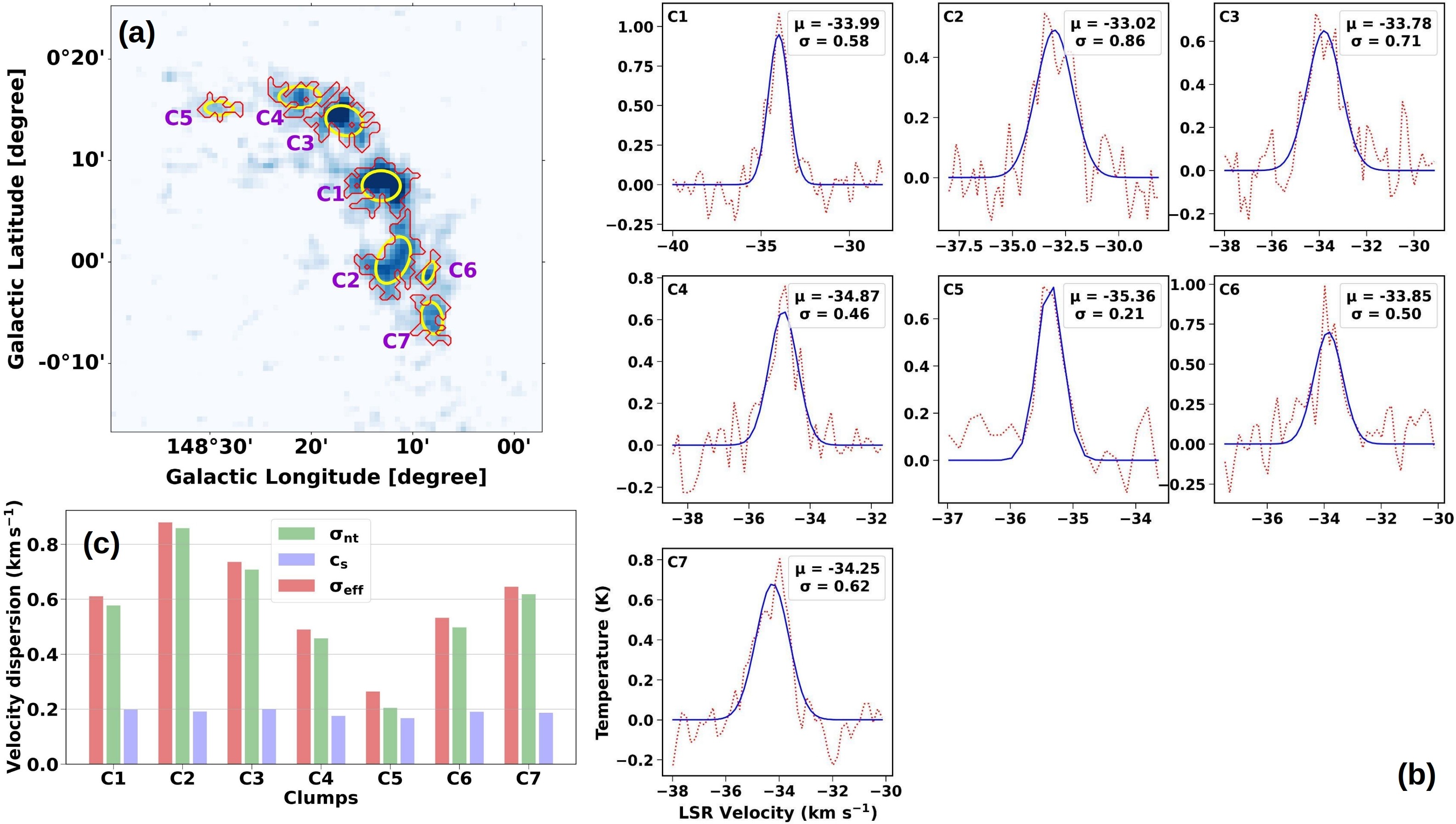
Figure 15: (a) The location of the clumps identified using ASTRODENDRO over C¹⁸O intensity map. The red contours show the leaf structures identified using dendrograms, and the ellipses show the clump within them. (b) The average C¹⁸O spectral profile of the clumps over which the solid blue curve denotes the best-fit Gaussian profile, and their respective mean and standard deviation are given in each panel. (c) The histogram plot of non-thermal ($\sigma_{\mathrm{nt}}$), thermal sound speed ($c_{\mathrm{s}}$), and the total effective ($\sigma_{\mathrm{eff}}$) velocity dispersion of the clumps.

3.3.2 Properties of the clumps

We estimated the mass of the clumps using the integrated intensity emission within the clump boundary, the average excitation temperature from the excitation temperature map shown in Fig. 5, and equations 4, 5, and 7 described in Section 3.1.2. The clumps are found to be massive with masses in the range 260$-$2100 M_⊙, with the most massive being the central clump, C1, associated with the hub of the cloud. The second most massive clump (C2) is of mass $\sim$ 1800 M_⊙. The mass of C2 is likely an upper limit, as the clump is possibly tracing the part of the filament that connects C1 and C2. The effective radius ($R_{\mathrm{eff}}$) of the clump is calculated as $\sqrt{ab}$, where a and b are the semi-major and semi-minor axes of the clump (given in Table 3). The $R_{\mathrm{eff}}$ of the clumps are found to be in the range 0.8$-$1.9 pc, with a mean value of $\sim$ 1.4 pc.

Velocity dispersion can reflect the level of turbulence in clumps, and the mean line-width, $\Delta V$ of the clump is related to the velocity dispersion ($\sigma_{\mathrm{obs}}$) as 2.35$\sigma_{\mathrm{obs}}$. We get the observed velocity dispersion by fitting a Gaussian profile over the C¹⁸O spectrum of the clumps. Fig. 15b shows the average spectral profile of all the clumps. The velocity dispersion of the clumps is in the range of 0.21 to 0.86 km s^-1, with a mean value of 0.56 km s^-1. As determined for the whole cloud, one can also infer whether the clumps are bound or not by calculating the virial parameter, $\alpha=\frac{M_{\mathrm{vir}}}{M_{\mathrm{c}}}$, where $M_{\mathrm{vir}}$ and $M_{\mathrm{c}}$ are the virial mass and gas mass of the clumps, respectively. We calculated $M_{\mathrm{vir}}$ using density index, $\beta$ = 2, by assuming a spherical density profile for the clumps. The $R_{\mathrm{eff}}$, mean T_ex, $\Delta V$, $M_{\mathrm{c}}$, and $\alpha$ values of the clumps are tabulated in Table 3. The $\alpha$ value of all the clumps is found to be less than 2, suggesting that they are gravitationally bound and, thus, would form or are in the process of forming stars. This will also remain true even if we take $\beta$ =1.5.

To determine the contribution of non-thermal (turbulent) support against gravity in the clumps, we calculate the non-thermal velocity dispersion and total effective velocity dispersion from the total observed velocity dispersion, using the same procedures outlined in Section 3.2.5. Fig. 15c shows the $\sigma_{\mathrm{nt}}$, $c_{\mathrm{s}}$, and $\sigma_{\mathrm{eff}}$ values of the clumps based on C¹⁸O data. From the figure, it can be seen that for all the clumps, the non-thermal velocity dispersion or the turbulence contribution is more dominant than the thermal component. Using the ratio $\sigma_{\mathrm{nt}}/c_{\mathrm{s}}$, we calculate the Mach number, which is given in Table 3. The Mach number lies in the range of 1.2 to 4.5, with a mean of around 3. Thus, the clumps have supersonic non-thermal motions. The non-thermal motions could be either due to small-scale gas motions within the clump or protostellar feedback due to local star formation activity or a combination of both the processes. For example, Rawat et al. (2023) discussed that the hub is also associated with a massive YSO (Young Stellar Object) with an outflow, thus, its radiation and feedback might have also impacted the dynamics of the surrounding gas.

4 Discussion

4.1 Stability of the Filaments

The stability of the filament can be evaluated by comparing its observed line mass, $M_{\mathrm{line}}$, with the critical line mass, $M_{\mathrm{crit}}$. Assuming filaments are in cylindrical hydrostatic equilibrium, $M_{\mathrm{crit}}$, is expressed as (Fiege & Pudritz, 2000):

$$M_{\mathrm{crit}}=\frac{2\sigma_{\mathrm{eff}}^{2}}{G}\sim 464\,\sigma_{\mathrm{eff}}^{2}\,(M_{\odot}\,pc^{-1}),$$ (10)

where $\sigma_{\mathrm{eff}}$ is the effective velocity dispersion in km s^-1and G is the gravitational constant. The filament is unstable to axisymmetric perturbation if its line mass exceeds its critical line mass (Inutsuka & Miyama, 1992). In the case of isothermal filament, $\sigma_{\mathrm{eff}}$ = c_s, where c_s is the sound speed of the medium (e.g. Ostriker, 1964). In this scenario, the critical line mass only depends on the gas temperature. The average temperature ($T_{\rm{ex}}$) of the filaments estimated within their widths lies in the range 8$-$10 K, which corresponds to $M_{\mathrm{crit}}$ $\sim$ 13$-$17 M_⊙ pc^-1. The line masses for the filaments that we estimated with our data are significantly above the critical thermal line mass. This suggests that either the filaments are collapsing radially or they are supported by additional mechanisms such as non-thermal turbulent motions. These turbulent motions can be generated either due to already formed stars within the filaments or by the radial accretion/infall of the surrounding gas onto the filaments (Hennebelle & André, 2013; Clarke et al., 2016). The presence of non-thermal motions would increase the effective sound speed, thereby would increase the effective velocity dispersion ($\sigma_{\mathrm{eff}}=\sqrt{c_{\mathrm{s}}^{2}+\sigma_{\mathrm{nt}}^{2}}$) of the filament, and thus, the critical line mass. At present, the observed velocity dispersion along the filament is higher than that one would expect for a cloud with a temperature in the range 10$-$15 K. Therefore, to understand the present dynamical status of the filaments, we compute the $M_{\mathrm{crit}}$ for the filaments assuming that they are supported by thermal as well as non-thermal motions. Using the mean effective velocity dispersion of the filaments (0.44, 0.45, 0.44, 0.68, 1.03, and 0.78 km s^-1), we calculated the $M_{\mathrm{crit}}$ values as 90, 94, 90, 215, 496, and 283 M_⊙ pc^-1 for F1, F2, F3, F4, F5, and F6, respectively, with a mean value around $\sim$ 211 M_⊙ pc^-1.

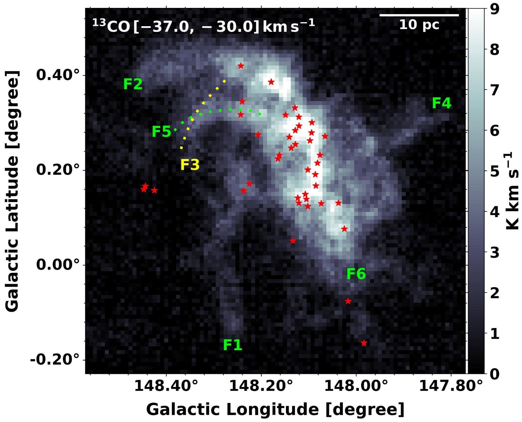
Figure 16: The distribution of protostars from $\it{Herschel}$ 70 micron point source catalogue (Herschel Point Source Catalogue Working Group et al., 2020) on the ¹³CO integrated intensity map.

Arzoumanian et al. (2019) based on $\it{Herschel}$ analysis and considering thermal line mass as the critical mass, categorised the filaments of the nearby clouds as supercritical filaments ($M_{\mathrm{line}}$ $\geq$ 2 $M_{\mathrm{crit}}$,), transcritical filaments (0.5 $M_{\mathrm{crit}}$ $\leq$ $M_{\mathrm{line}}$ $\leq$ 2 $M_{\mathrm{crit}}$ ), and subcritical filaments ($M_{\mathrm{line}}$ $\leq$ 0.5 $M_{\mathrm{crit}}$). They suggested that thermally subcritical filaments are gravitationally unbound entities, while transcritical and supercritical filaments are the preferable sites for gravitational collapse and core formation. Based on the thermal line mass, all of our filaments are super-critical, thus, might have undergone collapse and sub-sequence fragmentation to form cores. This fact is evident from the distribution of protostars on the filaments, shown in Fig. 16. The figure shows that most of the protostars have been formed in the ridge/F6 of the G148.24+00.41 cloud, and a few protostars seem to be formed at the head of the filaments F1, F2, and F5. Taking the contribution of non-thermal motion, we find that the line mass of F1, F2, F3, and F6 is larger than their $M_{\mathrm{crit}}$ values, suggesting that they are still gravitationally unstable, whereas for F4 and F5, the $M_{\mathrm{line}}$ is smaller than the $M_{\mathrm{crit}}$ value, suggesting that they are possibly stable against collapse. However, we note that the line masses are estimated with canonical values of $\mathrm{{}^{12}C}$ to $\mathrm{{}^{13}C}$ isotope ratio and can be higher by a factor of 1.3, if isotopic ratio at the galactocentric distance of the cloud is considered (e.g. Pineda et al., 2013).

In the above discussion, we have investigated the dynamical status of the filaments, however, we note that in the dynamical scenario of cloud formation and evolution, filaments are very likely to deviate from true equilibrium structures. Because in the dynamical scenario of cloud collapse, filaments are described as dynamical structures that continuously accrete from the ambient gas while feeding dense cores within them. Moreover, it has also been found that due to the gravitational focusing effect, finite filaments are more prone to collapse at the ends of their long axis (Burkert & Hartmann, 2004; Pon et al., 2011), even when such filaments are subcritical. Thus, though the average properties of some of the filaments are sub-critical, they have a higher concentration of column density at their heads due to longitudinal flow along their axis, where filaments can transit from sub-critical to super-critical.

4.2 Mass flow Along the Filament Axis

Assuming that the observed velocity gradient in filaments is due to gas accretion flow, we estimate the mass accretion rate, $\dot{M_{\parallel}}$ along the filaments using a simple cylindrical model and relation given in Kirk et al. (2013),

$$\dot{M_{\parallel}}=V_{\parallel}\times\rho(\pi r^{2})\ \ =\ \ V_{\parallel}\left(\frac{M}{L}\right),$$ (11)

where $V_{\parallel}$ is the velocity along the filament, which is multiplied by the density, $\rho=\left(\frac{M}{\pi r^{2}L}\right)$, and the perpendicular area ($\pi r^{2}$) of the flow. The r, M, and L are the radius, mass content, and length of the cylinder, respectively. By taking the plane of sky projection with an inclination angle, $\alpha$, the observed parameters of the cylinder are: $L_{\rm{obs}}=Lcos(\alpha)$, $V_{\parallel,\rm{obs}}=V_{\parallel}sin(\alpha)$, and $V_{\parallel,\rm{obs}}=\Delta V_{\parallel,\rm{obs}}L_{\rm{obs}}$. After simplification, the $\dot{M_{\parallel}}$ expression reduces to

$$\dot{M_{\parallel}}=\frac{\Delta V_{\parallel,\rm{obs}}M}{tan(\alpha)},$$ (12)

where, $\Delta V_{\parallel,\rm{obs}}$ is the observed velocity gradient along the filament. Taking the obtained mass and velocity gradient of the filaments (see Table 2), and $\alpha$ = 45$\degree$ (Kirk et al., 2013), the estimated mass accretion rate for filament F1, F2, F3, F4, F5, and F6 is around $\sim$ 140, 264, 26, 150, 204, and 207 M_⊙ Myr^-1, respectively. Among which, the filaments F2, F5, and F6 are directly tied to the hub (see Fig. 11), whose combined accretion rate is around $\sim$ 675 M_⊙ Myr^-1. We note that the combined mass-accretion rate to the hub is an upper limit as the F6 filament will not transfer its mass entirely to the central hub due to the presence of an additional clump competing with it in the filament. However, we have not accounted for the contribution of small-scale filaments attached to the hub, as seen in the $\it{Herschel}$ dust continuum image (Fig 14 of Rawat et al., 2023), which would conversely add to the combined accretion rate.

Taking the above-measured accretion rate as a face value, we find that it is either comparable or higher than some of the well-known cluster-forming hubs found in the literature, such as Mon R2 (400$-$700 M_⊙ Myr^-1, Treviño-Morales et al., 2019), Serpens (100$-$300 M_⊙ Myr^-1, Kirk et al., 2013), Orion (385 M_⊙ Myr^-1, Rodriguez-Franco et al., 1992; Hacar et al., 2017), the DR 21 ridge (1000 M_⊙ Myr^-1, Schneider et al., 2010), G326.27-0.49 (970 M_⊙ Myr^-1, Mookerjea et al., 2023), and G310.142+0.758 (700 M_⊙ Myr^-1, Yang et al., 2023). This comparison, however, should be treated with caution because all these measurements have been done with different tracers having different resolutions that cover different scales around the hubs. Measuring the accretion rate for massive clouds that have hub filamentary systems, such as those mentioned above, in a uniform way, would give more valuable insight into the accretion rate and the mass assembly time scales of such systems.

4.3 Overview of Cluster Formation Processes in G148.24+00.41

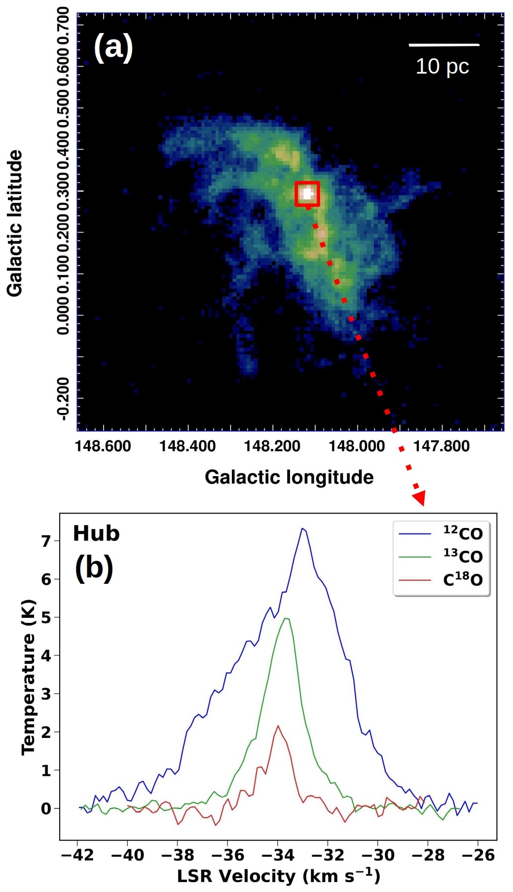
Figure 17: (a) The ¹³CO integrated intensity map showing the location of the hub by a red box, having size $\sim$ 3.5 $\times$ 3.0 pc. (b) The average $\rm{{}^{12}CO}$, $\rm{{}^{13}CO}$, and C¹⁸O spectral profile of the hub region (shown in panel a).

Rawat et al. (2023) studied the cloud’s profile, structure, and fractalness, as well as the spatial, temporal, and luminosity distribution of the protostars with respect to the cloud’s central potential, and suggested that the cloud is likely in a state of hierarchical collapse.

Vázquez-Semadeni et al. (2019) suggested that due to non-homologous collapse in molecular clouds, a classical signature of spherical collapse is not expected over a larger scale. However, at the clump scale, a global velocity offset between peripheral ¹²CO and internal ¹³CO , as found by Barnes et al. (2018), is a signature of collapse. According to Barnes et al. (2019), if the average ¹²CO profile is red-shifted with respect to the average ¹³CO profile, the motion of the enveloping ¹²CO gas is inwards, while if it is blue-shifted, then the motion is outwards. Fig. 17b shows the line profiles of the CO-molecules within the 3 pc area (marked by the red rectangle in Fig. 17a) around the hub. The figure shows that the ¹²CO profile is redshifted with respect to ¹³CO profile, inferring the net inward motion of ¹²CO envelope (Barnes et al., 2018). However, to get the conclusive signature of infall motion at the clump scale, we need high-density tracer data (Yuan et al., 2018; Liu et al., 2020; Yang et al., 2023).

In G148.24+00.41, there are six filaments with converging flows heading towards the hub of the cloud. For the filaments having aspect ratio, $\rm{A_{0}=Z_{0}/R_{0}}\gtrsim 2$, one can calculate the longitudinal collapse timescale using a single equation, $t_{\rm{COL}}\sim(0.49+0.26A_{0})(G\rho_{0})^{-1/2}$ (Clarke & Whitworth, 2015), where $\rm{Z_{0}}$, $\rm{R_{0}}$, and $\rho_{0}=M_{\rm{line}}/\pi\rm{R_{0}^{2}}$ is the half-length, radius, and density of the filament, respectively. In our case, the aspect ratio of all the filaments is greater than 2. Using the aforementioned formalism, we find that the longitudinal collapse timescale of these filaments is in the range of 5$-$15 Myr, while the free-fall time of the central clump ($t_{ff}=\sqrt{3\pi/32G\rho\rm{{}_{c}}}$, where $\rho\rm{{}_{c}}$ is the density of the clump) is found to be $\sim$1 Myr. Since in dynamical hierarchical collapse, each scale accretes from a larger scale, implying that the filaments may continue to fuel the clump for a longer time, provided that they remain bound. Taking the upper limit of combined inflow rate to the C1-clump as $\sim$ 675 M_⊙ Myr^-1, we estimate that to assemble the current mass of the clump, i.e. $\sim$ 2100 M_⊙, a minimum time of $\sim$3 Myr would be needed, while the age of the cloud based on formed young stellar objects is around 0.5$-$1 Myr (for details, see Rawat et al., 2023). This implies that while the mass assembly is ongoing towards the clump, the star formation in the cloud might have initiated around 0.5$-$1 Myr ago. However, we acknowledge that our estimated mass assembly time scale to the C1-clump can be an upper limit due to the following reasons: i) the accretion rate was higher during the early phase of cloud evolution, ii) overestimation of the clump mass due to low-resolution data, iii) missing the contribution of other small-scale filaments such as those seen in $\it{Herschel}$ images, or a combination of all. Future high-resolution observations focusing on the clump area would shed more light on the latter two hypotheses. None the less, the derived accretion rate is close to those found in some of the well-known cluster-forming hub-filamentary systems (discussed in Section 4.2) and also to the prediction of massive cluster-forming simulations (e.g. Vázquez-Semadeni et al., 2009; Howard et al., 2018). For example, Vázquez-Semadeni et al. (2009) using numerical simulations, suggest that the formation of massive stars or clusters is associated with large-scale collapse involving thousands of solar masses and accretion rates of $\sim$ 10^-3 M_⊙ yr^-1.

The G148.24+00.41 cloud has fragmented into seven massive clumps in the range of 260$-$2100 M_⊙, and the majority of them have the potential to form an independent group of stars or cluster (e.g. to form a massive star and associated cluster, a minimum mass $\geq$ 300 M_⊙ is needed; see Appendix A in Sanhueza et al., 2019). However, our search for the presence of embedded sources within the clumps using mid-infrared data (i.e. using 3.6 $\mu$m $\it{Spitzer}$ images) resulted that the massive clumps are associated with stellar sources, and the hub (i.e. the clump C1) hosts the most compact and richer stellar group. Rawat et al. (2023) also found that the most luminous ($\sim$ 1900 L_⊙) protostar of the complex is located within the hub. Thus, we hypothesize that in the G148.24+00.41 cloud, the cluster formation in the hub is facilitated by filamentary accretion flows from large-scale cloud to small-scale clumps/hub, which can either be gravity-driven (GHC; Gómez & Vázquez-Semadeni, 2014; Vázquez-Semadeni et al., 2019) or turbulence-driven (I2; Padoan et al., 2020). The cluster in the hub has the potential to grow into a richer cluster by gradually accumulating additional cold gas. Rawat et al. (2023), based on the spatial and temporal distribution and fractal subclustering of the stellar sources in G148.24+00.41, suggest that GHC may be the dominant mechanism responsible for the formation of the stellar cluster in this cloud. Based on the low-resolution CO data, used in this work, it is difficult to distinguish between the aforementioned two models. Future shock tracer observational data would be helpful in this regard, as the I2 model suggests the formation of filaments due to shocks, while in GHC, the filaments form due to large-scale gravity flow (Yang et al., 2023). Figure 18 illustrates the potential structure and overall gas kinematics of the cloud, forming clusters at the nodes of the filamentary flows, with the richest cluster being located at the bottom of the cloud’s potential.

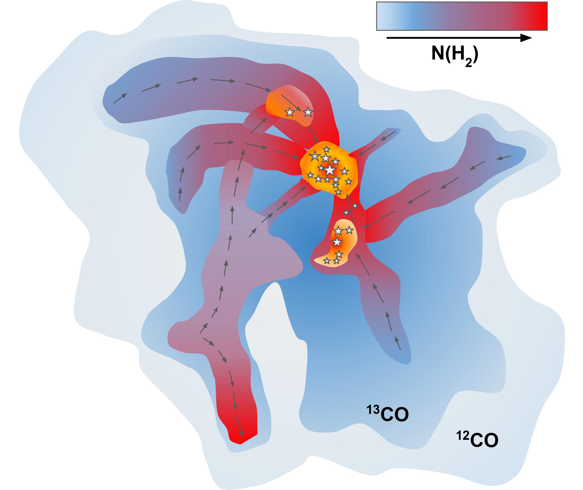
Figure 18: Cartoon illustrating the observed structures in G148.24+00.41. The black arrows represent the directions of the overall gas flow. The background colour displays the local density of ¹²CO and ¹³CO .

5 Summary and Conclusion

In the present work, we studied the gas properties and kinematics of the cloud. Based on CO analysis, we confirm that the cloud is massive ($\sim$ 10⁵ M_⊙), bound, and hosts a massive clump of mass $\sim$ 2100 M_⊙ nearly at its geometric centre. Based on the low-resolution ¹³CO data, in the present work, we identified six likely velocity coherent, large-scale (length $>$ 10 pc and aspect ratio $>$ 4) filamentary structures in the cloud. Out of which, three filaments (namely F2, F5, and F6) are directly tied to the clump located in the hub. We could not identify and characterize three relatively small-scale filaments that are attached to the hub as seen in the $\it{Herschel}$ images, thus, their role and properties are not investigated in this work. Among the studied filaments, we find that most of them are massive, with high mass per unit length, $M_{\rm{line}}$. We estimated that each filament has the potential to fuel the cold gaseous matter at a rate ranging from 26 to 264 M_⊙ Myr^-1 to the centre of the cloud.

The filaments have undergone fragmentation as several protostars (age $\leq$ 5 $\times$ 10⁵ yr) that are identified using 70 $\mu$m and 160 $\mu$m images by Rawat et al. (2023) are found to be associated with the filaments. Particularly, the filament F6 seems to be associated with a chain of protostars along its spine. The filament F6 has a high line mass, thus possibly actively forming protostars. In the case of the other filaments, the protostars are located close to their respective head, where strong density enhancement is seen in their respective integrated intensity map. These density enhancements could be due to the filamentary accretion flows along their long axis towards the bottom of the potential well, i.e. towards the hub location. In fact, the velocity profile of the filaments suggests that each filament is possibly undergoing longitudinal collapse, as the majority of them tend to show a velocity gradient in the range 0.03$-$0.06 km s^-1pc^-1. These gradients are derived over the entire length of the filaments, i.e. for the length scale of 10$-$15 pc and found to be comparable to the gradients of the large-scale filaments. We find that the increase in velocity along the filaments is also correlated with the increase in column density and velocity dispersion. We have also found higher velocity gradients near the hub location (see Fig. 14b), implying the acceleration of gas motion towards the hub. We note that, though the kinematic features are suggestive of large-scale flows toward the hub, but due to the presence of other clumps in the ridge, the kinematics of the filaments are found to be complicated. Future high-resolution observations will be essential to better understand the kinematics and dynamics of the gas in the filaments and the hub, and unveil the multi-scale process of massive cluster formation.

The cloud has fragmented into seven massive clumps having mass in the range 260$-$2100 M_⊙. We found that the clump located at the hub of the cloud is the most massive one, associated with a massive YSO and a stellar cluster. All these evidence suggests that within the cloud, the hub is the dominant place where a prominent cluster is in the process of emerging. Overall, our results are consistent with the flow-driven gas assembly, leading to the formation of the dense clump in the hub and the subsequent emergence of a stellar cluster.

Data Availability

We used the CO molecular data from PMO, which can be shared by the PMO database on reasonable request. We have also used Herschel 250 $\,\mu m$ image and 70 micron point source catalogue. The Herschel images are publicly available from Herschel Science Archive (http://archi ves.esac.esa.int/hsa/whsa) and the Herschel point source catalogue is available on Vizier.

Appendix A FilFinder Algorithm and Large-Scale Filaments

Figure 19: The filaments spines (red solid curve) of F1, F3, F4, F5, and F6 shown over there ¹³CO integrated intensity emission. The blue dots and perpendicular cuts (red solid lines) are the same as in Fig. 12a.

The $\it{FilFinder}$ package picks out the structures within a given mask by comparing each pixel to those in the surrounding neighbourhood using adapting thresholding. The algorithm then reduces the filament mask to skeletons using the Medial Axis Transform (MAT) method. Finally, it prunes down the skeleton structure to a filamentary network. $\it{Filfinder}$ not only extracts bright filaments but also reliably extracts fainter structures such as striations. We set the following optimum values in $\it{Filfinder}$ for creating mask and applying adapting thresholding, whose output matches better with the elongated structures visually seen in the column density map: i) global threshold, the intensities below this value are cut off from being included in the mask, as two times the background column density value, ii) adaptive threshold, the expected full width of filaments for adaptive thresholding, as 10 pixels (i.e. $\sim$ 5 times beam-width), iii) smooth size, used to smoothen the image to minimize the extraneous branches on the skeletons as 2 pixels (i.e. $\sim$ 1.0 times beam-width), iv) size threshold, the minimum dimensions expected for a filament as 100 pixels² (i.e. $\sim$ 20 times beam area). The emission structures were first flattened to 95 percentiles before applying the adapting thresholding to suppress the significantly brighter objects than filamentary structures such as dense cores.

Appendix B RadFil and Filament profiles

We employed $\it{RadFil}$ to find the filament radial profile, width, and other properties. $\it{RadFil}$ first smooths the filament spine and then makes perpendicular cuts to the tangent lines sampled evenly across the smoothed filament (see Fig. 12a and 19). Each cut is shifted to the peak intensity along the cut, which is marked by the blue dots in Fig. 12a and 19. Then, it computes the radial distances from the peak intensity point and the corresponding pixel intensities for each intersecting pixel along a given cut (see Zucker & Chen, 2018). In this way, $RadFil$ generates the intensity profile of each cut. Following the procedure, we made equidistant cuts perpendicular to the spine using a sampling frequency of 1 beam size. The radial profile at each cut was extracted, which gives an average profile or master profile of the filament and is shown in Fig. 12b and 20.

We identified the filament width (FWHM) by fitting a Gaussian function on the entire ensemble of the cuts. Before fitting the profile, a background was subtracted using the background subtraction estimator of $\it{RadFil}$ (Zucker & Chen, 2018). The background was estimated using the first-order polynomial for all the profiles at a given radial distance from the centre pixel (highest intensity pixel). The radial distance for background estimation is taken in the range where the observed intensity of the radial profile seems to be at a constant level for the filaments. The best-fit parameters are given in Table 2.

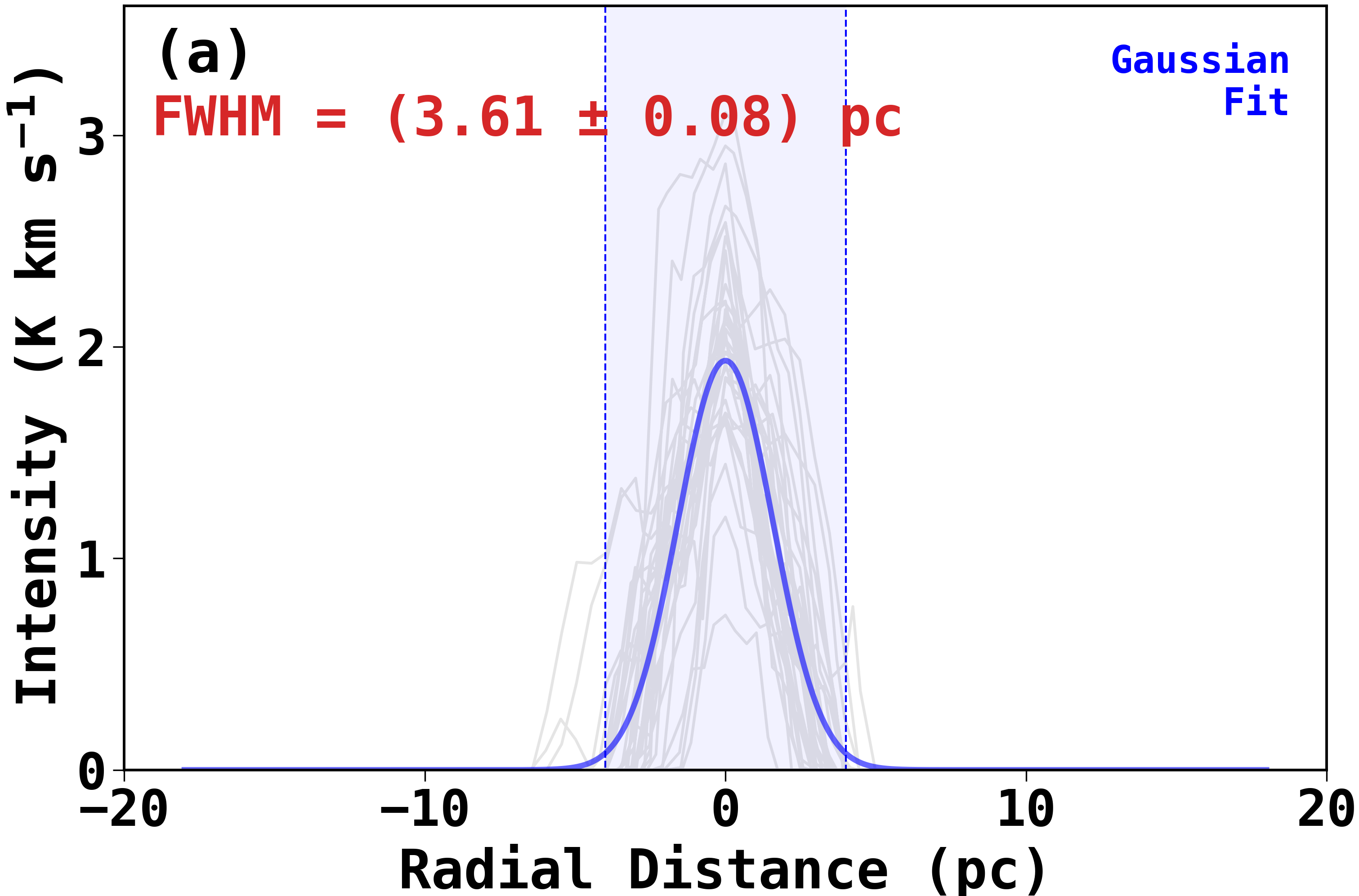
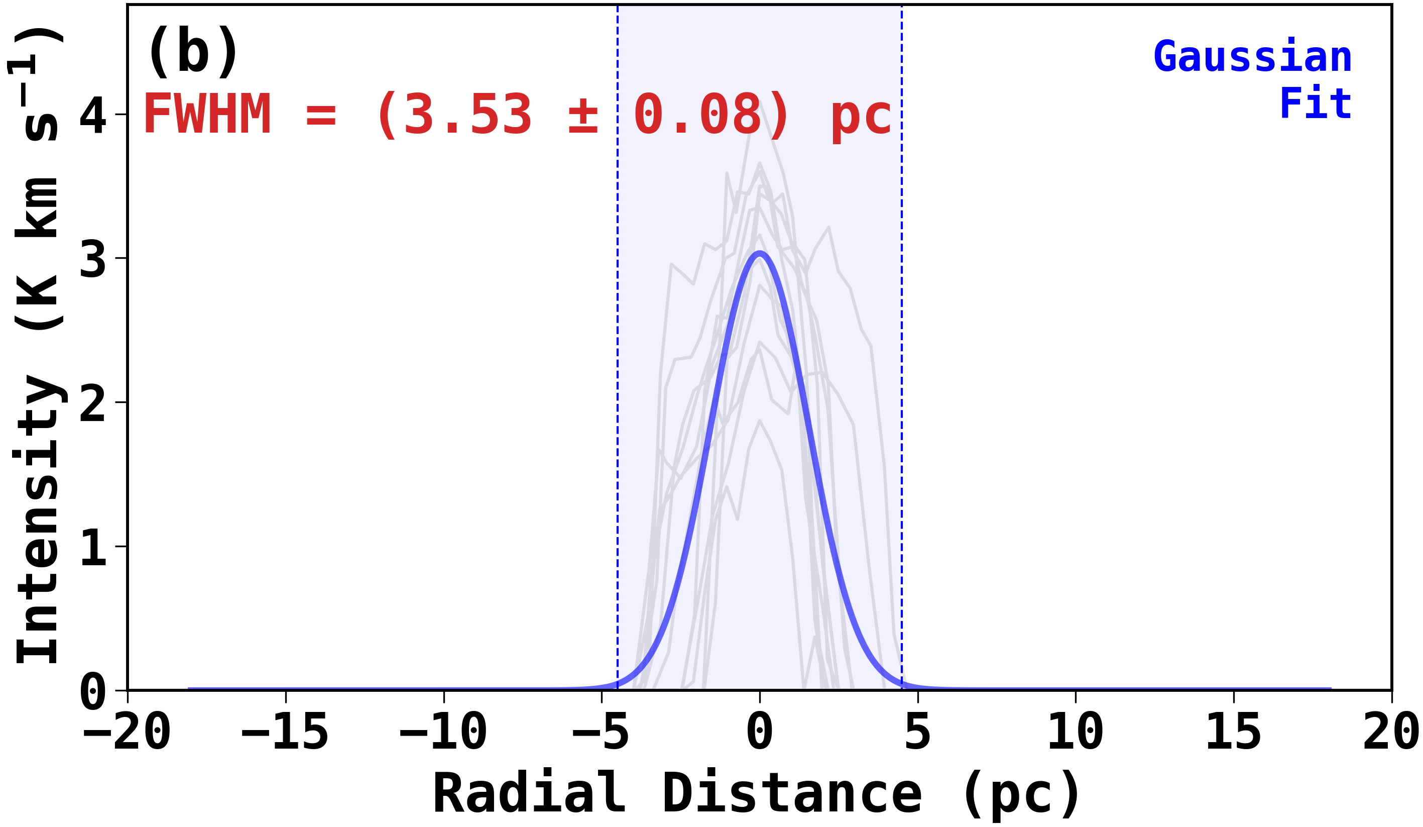
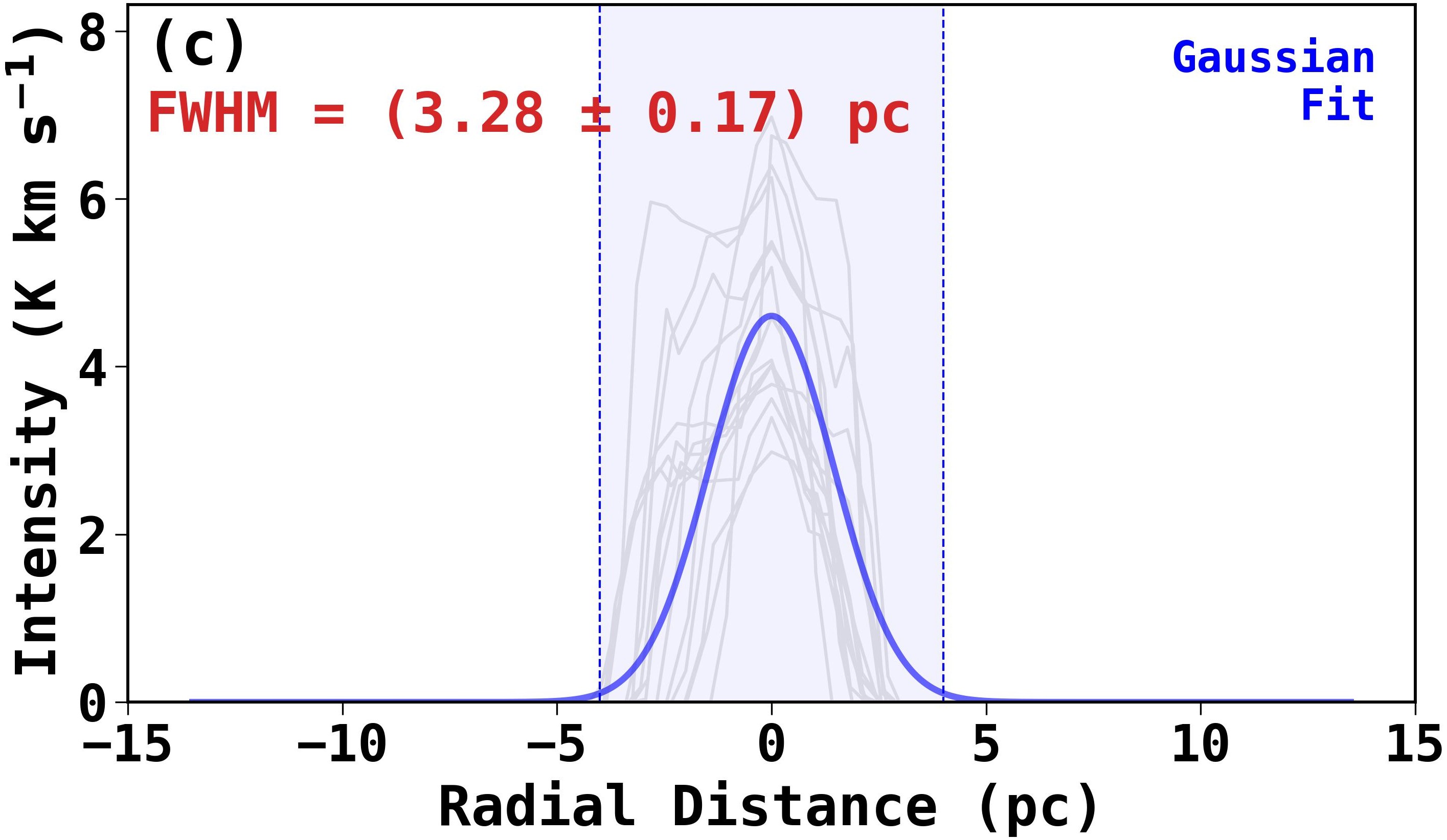
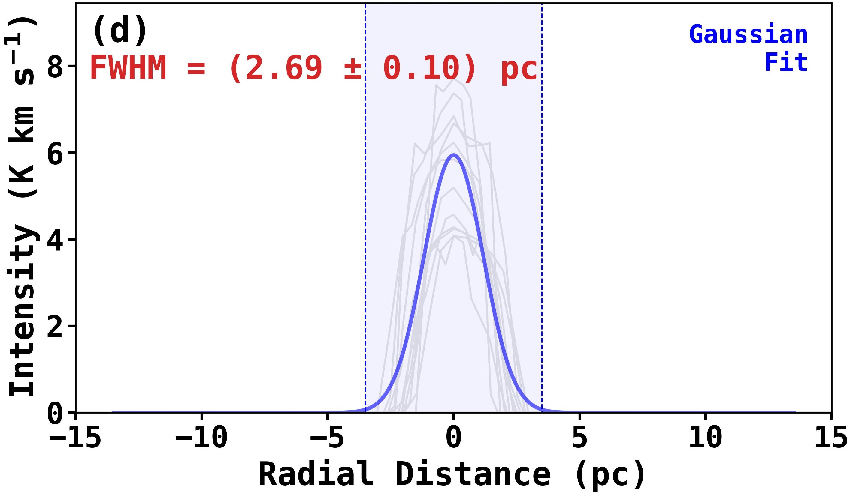
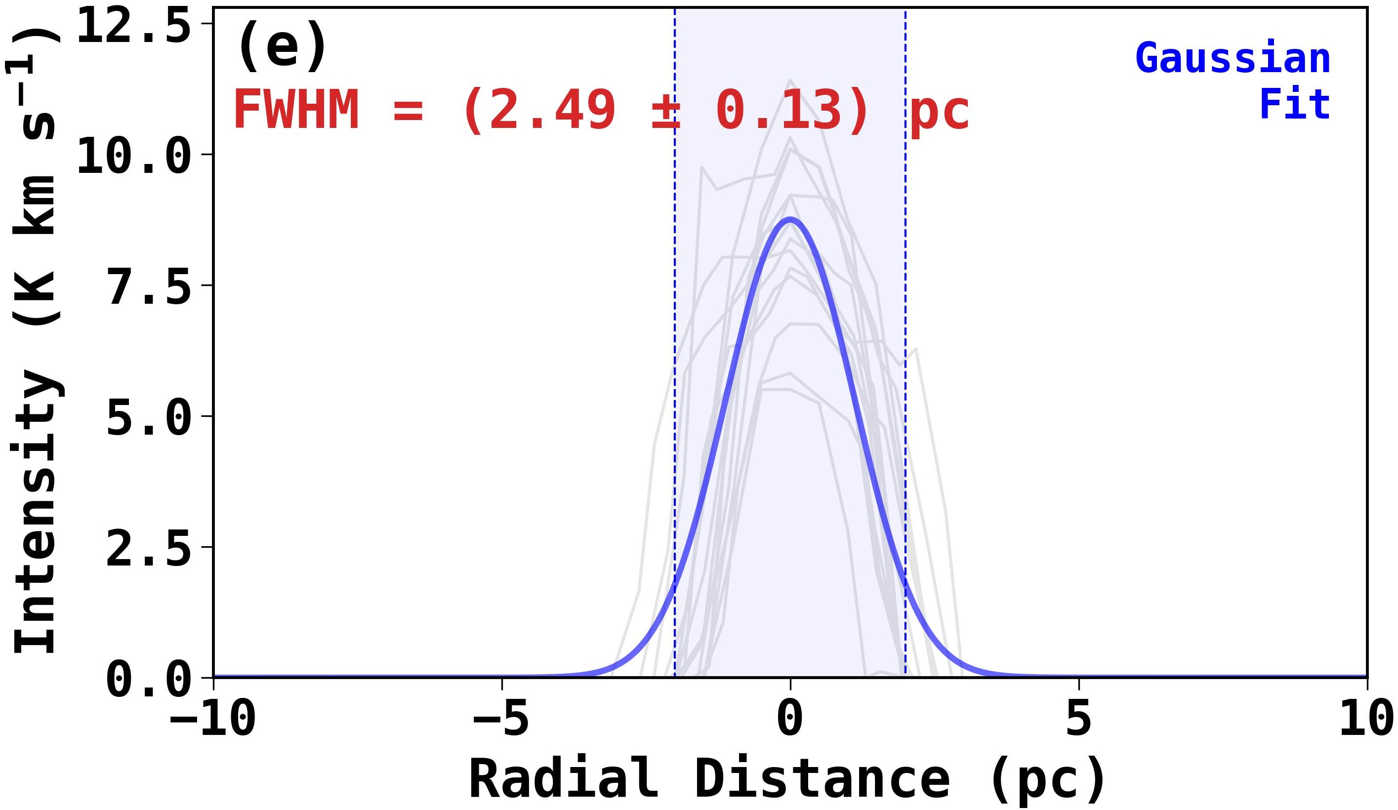
Figure 20: The radial profiles of perpendicular cuts along the filament spines of (a) F1, (b) F3, (c) F4, (d) F5, and (e) F6, with details same as in Fig. 12b.

References

- Adamo et al. (2020) Adamo A., et al., 2020, Space Sci. Rev., 216, 69
- André et al. (2010) André P., et al., 2010, A&A, 518, L102
- André et al. (2014) André P., Di Francesco J., Ward-Thompson D., Inutsuka S. I., Pudritz R. E., Pineda J. E., 2014, in Beuther H., Klessen R. S., Dullemond C. P., Henning T., eds, Protostars and Planets VI. p. 27 (arXiv:1312.6232), doi:10.2458/azu_uapress_9780816531240-ch002
- André (2017) André P., 2017, Comptes Rendus Geoscience, 349, 187
- Arzoumanian et al. (2019) Arzoumanian D., et al., 2019, A&A, 621, A42
- Banerjee & Kroupa (2015) Banerjee S., Kroupa P., 2015, MNRAS, 447, 728
- Barnes et al. (2018) Barnes P. J., Hernandez A. K., Muller E., Pitts R. L., 2018, ApJ, 866, 19
- Barnes et al. (2019) Barnes A. T., et al., 2019, MNRAS, 486, 283
- Beltrán et al. (2022) Beltrán M. T., Rivilla V. M., Kumar M. S. N., Cesaroni R., Galli D., 2022, A&A, 660, L4
- Bolatto et al. (2013) Bolatto A. D., Wolfire M., Leroy A. K., 2013, ARA&A, 51, 207
- Bourke et al. (1997) Bourke T. L., et al., 1997, ApJ, 476, 781
- Burkert & Hartmann (2004) Burkert A., Hartmann L., 2004, ApJ, 616, 288
- Cao et al. (2022) Cao Y., Qiu K., Zhang Q., Li G.-X., 2022, ApJ, 927, 106
- Carroll-Nellenback et al. (2014) Carroll-Nellenback J. J., Frank A., Heitsch F., 2014, ApJ, 790, 37
- Castets & Langer (1995) Castets A., Langer W. D., 1995, A&A, 294, 835
- Chen et al. (2020) Chen M. C.-Y., et al., 2020, ApJ, 891, 84
- Clarke & Whitworth (2015) Clarke S. D., Whitworth A. P., 2015, MNRAS, 449, 1819
- Clarke et al. (2016) Clarke S. D., Whitworth A. P., Hubber D. A., 2016, MNRAS, 458, 319
- Cox et al. (2016) Cox N. L. J., et al., 2016, A&A, 590, A110
- Dame et al. (2001) Dame T. M., Hartmann D., Thaddeus P., 2001, ApJ, 547, 792
- Dewangan et al. (2020) Dewangan L. K., Ojha D. K., Sharma S., Palacio S. d., Bhadari N. K., Das A., 2020, ApJ, 903, 13
- Federrath (2016) Federrath C., 2016, MNRAS, 457, 375
- Fiege & Pudritz (2000) Fiege J. D., Pudritz R. E., 2000, MNRAS, 311, 85
- Frerking et al. (1982) Frerking M. A., Langer W. D., Wilson R. W., 1982, ApJ, 262, 590
- Friesen et al. (2013) Friesen R. K., Medeiros L., Schnee S., Bourke T. L., di Francesco J., Gutermuth R., Myers P. C., 2013, MNRAS, 436, 1513
- Friesen et al. (2016) Friesen R. K., Bourke T. L., Di Francesco J., Gutermuth R., Myers P. C., 2016, ApJ, 833, 204
- Garden et al. (1991) Garden R. P., Hayashi M., Gatley I., Hasegawa T., Kaifu N., 1991, ApJ, 374, 540
- Goldsmith (2001) Goldsmith P. F., 2001, ApJ, 557, 736
- Goldsmith & Langer (1999) Goldsmith P. F., Langer W. D., 1999, ApJ, 517, 209
- Goldsmith et al. (2008) Goldsmith P. F., Heyer M., Narayanan G., Snell R., Li D., Brunt C., 2008, ApJ, 680, 428
- Gómez & Vázquez-Semadeni (2014) Gómez G. C., Vázquez-Semadeni E., 2014, ApJ, 791, 124
- Gómez et al. (2018) Gómez G. C., Vázquez-Semadeni E., Zamora-Avilés M., 2018, MNRAS, 480, 2939
- Guilloteau & Lucas (2000) Guilloteau S., Lucas R., 2000, in Mangum J. G., Radford S. J. E., eds, Astronomical Society of the Pacific Conference Series Vol. 217, Imaging at Radio through Submillimeter Wavelengths. p. 299
- Guo et al. (2022) Guo W., et al., 2022, ApJ, 938, 44
- Hacar et al. (2013) Hacar A., Tafalla M., Kauffmann J., Kovács A., 2013, A&A, 554, A55
- Hacar et al. (2016) Hacar A., Alves J., Burkert A., Goldsmith P., 2016, A&A, 591, A104
- Hacar et al. (2017) Hacar A., Alves J., Tafalla M., Goicoechea J. R., 2017, A&A, 602, L2
- Hacar et al. (2018) Hacar A., Tafalla M., Forbrich J., Alves J., Meingast S., Grossschedl J., Teixeira P. S., 2018, A&A, 610, A77
- Hacar et al. (2022) Hacar A., Clark S., Heitsch F., Kainulainen J., Panopoulou G., Seifried D., Smith R., 2022, arXiv e-prints, p. arXiv:2203.09562
- Heitsch et al. (2008) Heitsch F., Hartmann L. W., Slyz A. D., Devriendt J. E. G., Burkert A., 2008, ApJ, 674, 316
- Hennebelle & André (2013) Hennebelle P., André P., 2013, A&A, 560, A68
- Hennemann et al. (2012) Hennemann M., et al., 2012, A&A, 543, L3
- Hernandez & Tan (2015) Hernandez A. K., Tan J. C., 2015, ApJ, 809, 154
- Hernandez et al. (2011) Hernandez A. K., Tan J. C., Caselli P., Butler M. J., Jiménez-Serra I., Fontani F., Barnes P., 2011, ApJ, 738, 11
- Herschel Point Source Catalogue Working Group et al. (2020) Herschel Point Source Catalogue Working Group et al., 2020, VizieR Online Data Catalog, p. VIII/106
- Heyer & Dame (2015) Heyer M., Dame T. M., 2015, ARA&A, 53, 583
- Heyer et al. (2009) Heyer M., Krawczyk C., Duval J., Jackson J. M., 2009, ApJ, 699, 1092
- Howard et al. (2018) Howard C. S., Pudritz R. E., Harris W. E., 2018, Nature Astronomy, 2, 725
- Hu et al. (2021) Hu B., et al., 2021, ApJ, 908, 70
- Inutsuka & Miyama (1992) Inutsuka S.-I., Miyama S. M., 1992, ApJ, 388, 392
- Kauffmann et al. (2008) Kauffmann J., Bertoldi F., Bourke T. L., Evans N. J. I., Lee C. W., 2008, A&A, 487, 993
- Kirk et al. (2013) Kirk H., Myers P. C., Bourke T. L., Gutermuth R. A., Hedden A., Wilson G. W., 2013, ApJ, 766, 115
- Koch & Rosolowsky (2015) Koch E. W., Rosolowsky E. W., 2015, MNRAS, 452, 3435
- Könyves et al. (2015) Könyves V., et al., 2015, A&A, 584, A91
- Krause et al. (2020) Krause M. G. H., et al., 2020, Space Sci. Rev., 216, 64
- Krumholz & McKee (2020) Krumholz M. R., McKee C. F., 2020, MNRAS, 494, 624
- Krumholz et al. (2019) Krumholz M. R., McKee C. F., Bland-Hawthorn J., 2019, ARA&A, 57, 227
- Kumar et al. (2020) Kumar M. S. N., Palmeirim P., Arzoumanian D., Inutsuka S. I., 2020, A&A, 642, A87
- Kumar et al. (2022) Kumar M. S. N., Arzoumanian D., Men’shchikov A., Palmeirim P., Matsumura M., Inutsuka S., 2022, A&A, 658, A114
- Lada & Lada (2003) Lada C. J., Lada E. A., 2003, ARA&A, 41, 57
- Lada et al. (2010) Lada C. J., Lombardi M., Alves J. F., 2010, ApJ, 724, 687
- Lewis et al. (2022) Lewis J. A., Lada C. J., Dame T. M., 2022, ApJ, 931, 9
- Li et al. (2015) Li H., et al., 2015, The Astrophysical Journal Supplement Series, 219, 20
- Li et al. (2022) Li S., et al., 2022, ApJ, 926, 165
- Liszt (2017) Liszt H. S., 2017, ApJ, 835, 138
- Liu et al. (2012) Liu H. B., Jiménez-Serra I., Ho P. T. P., Chen H.-R., Zhang Q., Li Z.-Y., 2012, ApJ, 756, 10
- Liu et al. (2020) Liu T., et al., 2020, MNRAS, 496, 2790
- Liu et al. (2021) Liu X.-L., Xu J.-L., Wang J.-J., Yu N.-P., Zhang C.-P., Li N., Zhang G.-Y., 2021, A&A, 646, A137
- Liu et al. (2023) Liu H.-L., et al., 2023, MNRAS, 522, 3719
- Longmore et al. (2014) Longmore S. N., et al., 2014, in Beuther H., Klessen R. S., Dullemond C. P., Henning T., eds, Protostars and Planets VI. pp 291–314 (arXiv:1401.4175), doi:10.2458/azu_uapress_9780816531240-ch013
- Mattern et al. (2018) Mattern M., et al., 2018, A&A, 619, A166
- Miville-Deschênes et al. (2017) Miville-Deschênes M.-A., Murray N., Lee E. J., 2017, ApJ, 834, 57
- Molinari et al. (2010) Molinari S., et al., 2010, A&A, 518, L100
- Mookerjea et al. (2023) Mookerjea B., Veena V. S., Güsten R., Wyrowski F., Lasrado A., 2023, MNRAS, 520, 2517
- Motte et al. (2018) Motte F., Bontemps S., Louvet F., 2018, ARA&A, 56, 41
- Myers (2009) Myers P. C., 2009, ApJ, 700, 1609
- Nakanishi & Sofue (2006) Nakanishi H., Sofue Y., 2006, PASJ, 58, 847
- Naranjo-Romero et al. (2012) Naranjo-Romero R., Zapata L. A., Vázquez-Semadeni E., Takahashi S., Palau A., Schilke P., 2012, ApJ, 757, 58
- Nishimura et al. (2015) Nishimura A., et al., 2015, ApJS, 216, 18
- Ostriker (1964) Ostriker J., 1964, ApJ, 140, 1056
- Padoan et al. (2020) Padoan P., Pan L., Juvela M., Haugbølle T., Nordlund Å., 2020, ApJ, 900, 82
- Panopoulou et al. (2017) Panopoulou G. V., Psaradaki I., Skalidis R., Tassis K., Andrews J. J., 2017, MNRAS, 466, 2529
- Panopoulou et al. (2022) Panopoulou G. V., Clark S. E., Hacar A., Heitsch F., Kainulainen J., Ntormousi E., Seifried D., Smith R. J., 2022, A&A, 657, L13
- Patra et al. (2022) Patra S., II N. J. E., Kim K.-T., Heyer M., Kauffmann J., Jose J., Samal M. R., Das S. R., 2022, The Astronomical Journal, 164, 129
- Peretto et al. (2014) Peretto N., et al., 2014, A&A, 561, A83
- Pineda et al. (2008) Pineda J. E., Caselli P., Goodman A. A., 2008, ApJ, 679, 481
- Pineda et al. (2010) Pineda J. L., Goldsmith P. F., Chapman N., Snell R. L., Li D., Cambrésy L., Brunt C., 2010, ApJ, 721, 686
- Pineda et al. (2013) Pineda J. L., Langer W. D., Velusamy T., Goldsmith P. F., 2013, A&A, 554, A103
- Pineda et al. (2022) Pineda J. E., et al., 2022, arXiv e-prints, p. arXiv:2205.03935
- Pon et al. (2011) Pon A., Johnstone D., Heitsch F., 2011, ApJ, 740, 88
- Ragan et al. (2014) Ragan S. E., Henning T., Tackenberg J., Beuther H., Johnston K. G., Kainulainen J., Linz H., 2014, A&A, 568, A73
- Rawat et al. (2023) Rawat V., et al., 2023, MNRAS, 521, 2786
- Rodriguez-Franco et al. (1992) Rodriguez-Franco A., Martin-Pintado J., Gomez-Gonzalez J., Planesas P., 1992, A&A, 264, 592
- Roman-Duval et al. (2010) Roman-Duval J., Jackson J. M., Heyer M., Rathborne J., Simon R., 2010, ApJ, 723, 492
- Romero & Cappa (2009) Romero G. A., Cappa C. E., 2009, MNRAS, 395, 2095
- Rosolowsky et al. (2008) Rosolowsky E. W., Pineda J. E., Kauffmann J., Goodman A. A., 2008, ApJ, 679, 1338
- Saha et al. (2022) Saha A., et al., 2022, MNRAS, 516, 1983
- Sanhueza et al. (2019) Sanhueza P., et al., 2019, ApJ, 886, 102
- Savage et al. (2002) Savage C., Apponi A. J., Ziurys L. M., Wyckoff S., 2002, ApJ, 578, 211
- Schisano et al. (2014) Schisano E., et al., 2014, ApJ, 791, 27
- Schneider et al. (2010) Schneider N., Csengeri T., Bontemps S., Motte F., Simon R., Hennebelle P., Federrath C., Klessen R., 2010, A&A, 520, A49
- Schuller et al. (2021) Schuller F., et al., 2021, MNRAS, 500, 3064
- Shan et al. (2012) Shan W., et al., 2012, IEEE Transactions on Terahertz Science and Technology, 2, 593
- Shimajiri et al. (2015) Shimajiri Y., et al., 2015, ApJS, 217, 7
- Shimajiri et al. (2019) Shimajiri Y., André P., Palmeirim P., Arzoumanian D., Bracco A., Könyves V., Ntormousi E., Ladjelate B., 2019, A&A, 623, A16
- Smith et al. (2014) Smith R. J., Glover S. C. O., Klessen R. S., 2014, MNRAS, 445, 2900
- Su et al. (2019) Su Y., et al., 2019, ApJS, 240, 9
- Suri et al. (2019) Suri S., et al., 2019, A&A, 623, A142
- Tigé et al. (2017) Tigé J., et al., 2017, A&A, 602, A77
- Treviño-Morales et al. (2019) Treviño-Morales S. P., et al., 2019, A&A, 629, A81
- Urquhart et al. (2008) Urquhart J. S., et al., 2008, A&A, 487, 253