Learning Persistent Community Structures in Dynamic Networks
via Topological Data Analysis

Abstract

Dynamic community detection methods often lack effective mechanisms to ensure temporal consistency, hindering the analysis of network evolution. In this paper, we propose a novel deep graph clustering framework with temporal consistency regularization on inter-community structures, inspired by the concept of minimal network topological changes within short intervals. Specifically, to address the representation collapse problem, we first introduce MFC, a matrix factorization-based deep graph clustering algorithm that preserves node embedding. Based on static clustering results, we construct probabilistic community networks and compute their persistence homology, a robust topological measure, to assess structural similarity between them. Moreover, a novel neural network regularization TopoReg is introduced to ensure the preservation of topological similarity between inter-community structures over time intervals. Our approach enhances temporal consistency and clustering accuracy on real-world datasets with both fixed and varying numbers of communities. It is also a pioneer application of TDA in temporally persistent community detection, offering an insightful contribution to field of network analysis. Code and data are available at the public git repository: https://github.com/kundtx/MFC_TopoReg

Introduction

Community detection on dynamic networks is crucial for graph analysis. The formation of social ties, economic transactions, the unfolding of human mobility and communication, such real-world events all lie in the identification of meaningful substructures and their evolution hidden in the temporal complex system. Static community detection algorithms are well-researched and developed, such as the Louvain method (Blondel et al. 2008), submodularity (Liu et al. 2013), and spectral clustering (Ng, Jordan, and Weiss 2001). As graph neural networks have shown super capabilities in fields such as node classification and link prediction, deep graph clustering methods have come to the fore (Zhou et al. 2022) and been gradually adopted in static community detection (Su et al. 2022). However, dynamic community detection methods are still slow to develop due to the lack of a clear definition of communities in dynamic networks. Some dynamic community detection algorithms apply improved static algorithms on each snapshot of the network (Javed et al. 2018). Nevertheless, these methods focus on snapshot optimal solutions and their results lack consistency in time.

Figure 1: Inconsistent inter-community structure in dynamic community detection. The top row shows three snapshots of a dynamic graph constructed at the vertex level, undergoing a transient perturbation; Different node colors represent their true community labels. The inconsistent communities are outlined by rectangles. The second row shows the corresponding community-level networks, which exhibit a falsely detected merge.

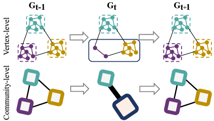
In many dynamic community detection scenarios, it is reasonable to assume that changes in the relationship between communities occur smoothly and the inter-community structure remains relatively stable over time. Research has shown that the structure of the network itself does not change significantly over a short period of time (Corne, Handl, and Knowles 2010). Moreover, the lack of temporal consistency in dynamic community detection makes it difficult to distinguish real community evolution from network perturbation, posing challenges for subsequent matching and analysis. For example, Fig. 1 illustrates an inconsistent community detection results in a simple network with three true communities, e.g. social groups. In the second time step, some perturbations, such as temporary changes in membership or interactions, would cause algorithms to incorrectly infer a merging event between two communities even though they return to being relatively independent in the next time step. A good dynamic community detection algorithm can correct the clustering results based on information from nearby snapshots. Similar motivations can be found in previous work such as ESPRA (Wang, Gao, and Ma 2017), which introduces quantum physics to model graph perturbations. While they try to smooth the structural perturbations at the vertex level, we focus on the stability at the community level. The community networks shown in the second row of Fig. 1 is a good model of the inter-community structure, where each node is a community and the weights of the edges are equal to the sum of the weights of the inter-community edges. Focusing on the community-level structure has a more direct impact on clustering results than simply modifying individual nodes and edges. In this paper, we investigate how to constrain the structural consistency of community networks within nearby snapshots.

We believe that the key to distinguishing inter-community structures lies in the topological characteristics of community networks. For example, in Fig. 1, the difference between a triangle and a line illustrates the difference in the structure of community networks. Since 2009, there have been increasing research efforts on Topological Data Analysis (TDA), which integrates algebraic geometry, computational geometry and data mining (Carlsson 2009). TDA characterizes intrinsic, topological changes in graph data through persistence homology, which quantify the topological features in the data across continuous scales. Topological graph analysis is a special class of TDA for graph data. Unlike heuristically designed topological features, such as the RA index (Zhou, Lü, and Zhang 2009), persistence homology is much more scale-independent and robust to perturbations, making it a better choice for quantifying the structural similarity in community networks.

In this work, we propose a novel dynamic community detection framework, which jointly performs graph clustering at the vertex-level and temporal consistency regularization at the community-level. Specifically, we solve two main challenges. First, the widely used self-supervised clustering module (Xie, Girshick, and Farhadi 2016) would collapse local structure of embedding distribution (Guo et al. 2017). To preserve the structure of the embedding space, we propose a novel deep graph clustering algorithm called MFC, which inspired by non-negative matrix factorization. The second challenge lies in how to incorporate the TDA-based consistency constraints on the community-level structures with vertex-level graph clustering methods. In this work, we design a differentiable operator that associates topological features with the cluster assignment distribution in deep clustering algorithms. Thus, the gradient of our Topological Regularization (TopoReg) can be back-propagated to the clustering module to penalize the topological differences in the community structure in neighboring snapshots.

The main contributions of our work are concluded as follows:

• We introduce topological graph analysis into dynamic community detection to learn consistent inter-community structures end-to-end.

• We propose a novel deep clustering algorithm that implements matrix factorization with relaxed sparsity constraints via neural networks.

• We empirically demonstrate the superiority of our proposed clustering algorithm and the importance of community structure preservation in dynamic community detection with both fixed and varying numbers of communities.

Related Works

Deep Graph Clustering

Deep graph clustering, clustering nodes in a graph into communities, is an emerging field in machine learning and social networks. We divide existing deep graph clustering methods into two classes: Static graph clustering or Dynamic graph clustering.

Static graph clustering. Most frameworks perform clustering on lower-dimensional embedding of graphs, based on popular architectures like GANs (Creswell et al. 2018), and Graph Auto-Encoders (Kipf and Welling 2016). A naive approach would directly perform traditional community detection methods on node embedding. EGAE (Zhang et al. 2022), a work very similar to our approach, is a typical one. It finds an ideal space for the clustering, but still uses $k$-means. Instead, another self-optimized deep clustering framework jointly optimizes the learned embedding and perform clustering, such as DAEGC (Wang et al. 2019). Their core clustering module comes from DEC (Xie, Girshick, and Farhadi 2016). Recent models improve deep graph clustering by better learning of node features, i.e. SCDN (Bo et al. 2020), AGCN (Peng et al. 2021) and DCRN (Liu et al. 2022), but the core clustering module does not change.

Dynamic graph clustering. Although there have been successful studies on evolving graphs, they mostly focus on node classification (Pareja et al. 2020) or temporal networks clustering, which typically yields a single clustering result for networks with changing edge weights (Liu et al. 2023). In contrast, this paper focuses on tracking community changes over discrete snapshots, which is relatively underexplored in the field. Traditional dynamic community detection algorithms, such as RTSC (You et al. 2021), ESPRA (Wang, Gao, and Ma 2017), DECS (Liu et al. 2020), often solve a multi-objective optimization problem. CGC (Park et al. 2022) improves the graph clustering algorithm based on contrastive learning and extends it to dynamic graphs, but its experiments are performed on a dataset with binary labels only. Dynamic graph embedding algorithms combine recurrent neural network with graph autoencoders, such as DynAE, DynRNN, and DynAERNN (Goyal, Chhetri, and Canedo 2020). Though without a dedicated clustering module, some clustering functionality is available.

Topological Graph Analysis

TDA can be extended to graphs by representing them as simplicial complexes, which encode their topology and structural properties. Numerous graph filtration methods have been proposed methods to compute persistent homology of graphs, such as Vietoris-Rips filtration (Dey and Wang 2022), weighted simplex filtration (Huang and Ribeiro 2016), and vertex-based clique filtration (Rieck et al. 2017). The graph topological features extracted from these graph filtration methods are widely used in biological and social graph data, among others. A series of studies on brain networks using TDA were presented by Songdechakraiwut and Chung (Songdechakraiwut and Chung 2023), such as learning MRI signals by graph filtration to understand complex relations in brain networks. Periodic phenomena in temporal traffic networks were studied using WRCF by Lozeve (Lozeve 2018), while Hajij (Hajij et al. 2018) uses Rips filtration to visualize structural changes in dynamic networks. In addition, recent works (Yan et al. 2021) have shown that adding topological graph analysis into GNNs can effectively improve their learning ability and performance.

Notations and Problem Formulation

Given a graph $G=(V,E)$, $V$ is a set of vertices and $E$ is a set of tuples $\left(u,v\right)$ with $u,v\in V$. A Dynamic Graph $\mathcal{G}_{\tau}$ is defined by an ordered set $\{G^{(1)},G^{(2)},\ldots,G^{(t)}\}$. Dynamic community detection is to find the best cluster assignment $Y^{(t)}$ for each snapshot $G^{(t)}$ at time step $t$. The criteria we define for good dynamic community detection are twofold: on the one hand, we need to achieve cohesive clustering results at each snapshot, and on the other hand, we expect the structure of the detected communities to maintain a certain degree of topological stability and continuity during dynamic changes of the input network. Our methods provide a trade-off between snapshot coherence and temporal consistency.

Methodology

In this section, we present our topology preserving dynamic community detection framework in detail. First, we will start by introducing a novel static deep graph clustering algorithm, followed by the topological consistency regularization for communities derived from clustering result within neighboring time windows. Note that we omit the time dimension in the Matrix Factorization Clustering section to make the notations more readable.

Matrix Factorization Clustering

Node embeddings learned by common deep clustering method tend to collapse to cluster centroids, which is desirable for node label inference but difficult to train in the presence of regularization. For example, DEC works by taking the proximity between the node embeddings and each cluster centers in the embedding space as the cluster assignment distribution. By constraining the sparsity of the distribution, the samples in each cluster are clustered toward the center. However, there is no guarantee that the samples near the margin will be pulled into the correct cluster, and it will destroy the structure of embedding space to some extent. Therefore, we propose a novel end-to-end deep graph clustering algorithm. It is called Matrix Factorization Clustering (MFC), a novel end-to-end deep graph clustering algorithm that learns relaxed matrix factorization on node embeddings using a Graph Auto-encoder (GAE). In contrast to DEC, MFC is a dimension reduction technique that avoids lossy compression, thereby preserving the structure of the embedding space. GAE incorporates the traditional auto-encoder and different kinds of GNNs, such as GCNs (Zhang et al. 2019) and GAT (Salehi and Davulcu 2020). Like a common auto-encoder, GAE consists of an encoder and a decoder. The encoder part attempts to learn a latent representation $Z=[\boldsymbol{z}_{1},\boldsymbol{z}_{2},...,\boldsymbol{z}_{n}]^{\mathrm{T}}$ of graph input with $n$ nodes via GNN layers. While the decoder intends to reconstruct the adjacency matrix $A$ from embedding $Z$, it is usually designed as $\sigma(ZZ^{\mathrm{T}})$ where $\sigma(\cdot)$ denotes the sigmoid function. The reconstruction loss $\mathcal{L}_{gae}$ is the binary cross entropy loss between $A$ and $\sigma(ZZ^{\mathrm{T}})$. In general, the clustering results can be obtained by directly performing $k$-means or other heuristic algorithms on embedding $Z$. However, the clustering results obtained in this way are not differentiable, so it is difficult to further optimize the topology of the detected community structure.

Figure 2: Framework of matrix factorization clustering. It consists of a graph auto-encoder and a clustering module.

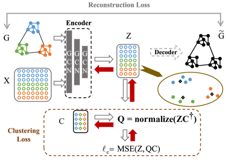
Matrix factorization has been proven to be essentially equivalent to $k$-means, spectral clustering, and many other clustering algorithms (Du et al. 2023). In our method, with relaxed sparsity constraints, Neural networks can be used to learn two low-rank matrices decomposed from the embedding matrix. Specifically, the optimization problem solved by $k$-means can be expressed as:

$$\min_{C,Q}\left\|Z-QC\right\|_{F}^{2},$$ (1)

$$\text{ s.t. }q_{ij}\in\{0,1\},Q\mathbf{1}_{k}=\mathbf{1}_{n}.$$

where $Q=(q_{ij})$ and $C=[\boldsymbol{\mu}_{1},\boldsymbol{\mu}_{2},...,\boldsymbol{\mu}_{k}]^{\mathrm{T}}$. $\boldsymbol{\mu}_{j}$ denotes center of $j$ cluster and $q_{ij}$ is the indicator. Specifically speaking, $q_{ij}=1$ if the $i$-th point is assigned to the $j$-th cluster. Otherwise, $q_{ij}=0$. The above problem is hard to solve directly due to the discrete constraint on $Q$. We first derive the closed-form solution of $Q$ in the unconstrained situation when $C$ is fixed. The objective function can be derived as:

$$\mathcal{J}_{km} =\left\|Z-QC\right\|_{F}^{2}$$ (2)

$$=\operatorname{tr}\left(Z^{\mathrm{T}}Z\right)-2\operatorname{tr}\left(Z^{\mathrm{T}}QC\right)+\operatorname{tr}\left(C^{\mathrm{T}}Q^{\mathrm{T}}QC\right).$$

Take the derivative of $\mathcal{J}_{km}$ and set it to 0

$$\nabla_{Q}\mathcal{J}_{km}=2(QCC^{\mathrm{T}}-ZC^{\mathrm{T}})=0$$ (3)

$$Q=ZC^{\mathrm{T}}(CC^{\mathrm{T}})^{-1}=ZC^{\dagger}$$

Inspired by Pseudo Inverse Learning (Guo and Lyu 2004) and ADMM (Alternating Direction Method of Multipliers) (Boyd et al. 2011), we consider $C$ as a set of weights in the neural network, thus combining the alternating optimization of $C$ and $Q$ with the training process. Specifically, $Q$ is updated by $Q=g(ZC^{\dagger})$ in forward propagation, the encoder of GAE and $C$ are updated by gradient descent in backward propagation. Here $g$ is a function that project $Q$ to the feasible region. Specifically, we relax the discrete constraints on $Q$ to a soft assignment problem, which means $q_{ij}\in(0,1),\sum_{j=1}^{k}q_{ij}=1$. Normalized by Softmax, Min-Max Normalization or other algorithms, any continuous matrix can satisfy the condition. In this paper we choose Min-Max Normalization to normalize each row $q$ of $Q$ as the relaxed constraints:

$$g(q)=\frac{q-\min(q)}{\max(q)-\min(q)}$$ (4)

The MSE (Mean Square Error) between $Z$ and $g(Q)C$ is calculated as $\mathcal{L}_{c}$ to jointly train the neural network with $\mathcal{L}_{gae}$ using back propagation until convergence. The detailed learning procedure of MFC is shown in Algorithm 1. When the best clustering centers $C^{*}$ is learned, the index of row maximum in $Q^{*}$ can be taken as the final clustering result of each node: $y_{i}=\arg\max_{u}q_{iu}$. One limitation of MFC is that since the principle of the method is matrix decomposition, the algorithm fails when the dimension of the node embeddings is less than the number of clusters. Because when the dimension of a matrix is greater than its rank, its pseudo-inverse does not exist.

Algorithm 1 Optimizing clustering module in MFC

Input: Node embedding matrix $Z$ of graph $G$ learned by GAE
Parameter: Trade-off parameter $\alpha$

1:  Initialize weights $C$ .

2:  repeat

3:     Calculate $Q=ZC^{\dagger}$.

4:     Normalize each row of $Q$ with function $g$.

5:     Calculate the differentiable clustering loss $\mathcal{L}_{c}=MSE(Z,g(Q)C)$ .

6:     Calculate the total loss and its gradients: $\mathcal{L}_{gae}+\alpha\times\mathcal{L}_{c}$.

7:     Update GAE weights and $C$ by gradient descent.

8:  until convergence or exceeding maximum iterations

9:  Ensure Assignment Matrix $Q$, clustering centers $C$ and GAE encoder parameters $\{W_{i}\}_{i=1}^{L}$

Topological Regularization of Dynamic Clustering Consistency

We propose an end-to-end regularization TopoReg to ensure the topological consistency of the community networks, which makes the clustering results more accurate and stable. It is a sliding window style loss function in order to reduce the topological distance between neighboring community networks. Furthermore, to feed the gradient back into the deep graph clustering module, we devise an elaborated community network construction method to make the community topology a differentiable function of cluster membership. The complete process is shown in Fig.3.

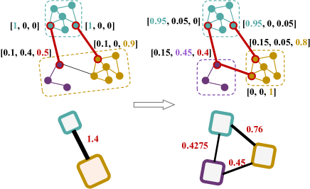
Construction of Community Topology. Given a graph $G$, the cluster assignment distribution $Q$ is computed in most deep graph clustering method such as DAEGC and the MFC algorithm we proposed. We can always assign a pseudo label $s_{i}$ on each node $i$ based the index of maximum row value of $Q$. This pseudo division of $G$ could form a new graph containing community structure called community network, whose nodes are communities. The weight of an edge connecting two communities A and B is determined by summing up the weights of all the edges that have one end belongs to A and the other belongs to B. The following equations demonstrate the derivation of community network based on $Q$ and the weighted adjacency matrix $W$ of $G$.

Figure 3: Illustration of topological regularization. A sequential process across three time steps is shown. Rows trace graph evolution with columns showing snapshots, embeddings, community graphs, and persistence barcodes. Different colors are used to differentiate the real category labels. Red arrows highlight the temporal consistency loss on persistence barcodes and the backpropagation path for the $t$th snapshot $G_{t}$.

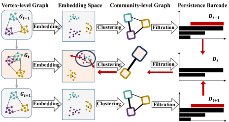
The pseudo label of node $i$ is $s_{i}=\arg\max_{k}(Q_{ik}),\forall i\in\{1,2,\ldots,n\}$. Assuming that graph $G$ has $K$ ground truth clusters, we have $s_{i}\in\{1,2,\dots,K\}$. Organize the pseudo-labels of all nodes into a vector $S=[s_{1},s_{2},\cdots,s_{n}]$, we define the indicator function $\mathbf{1}\left(S=k\right)=[\mathbf{1}\left(s_{1}=k\right),\mathbf{1}\left(s_{2}=k\right),\ldots,\mathbf{1}\left(s_{n}=k\right)]^{\mathrm{T}}=[0,0,\ldots 1,\ldots 0]^{\mathrm{T}}$, where $\mathbf{1}\left(s_{i}=k\right)=1.\iff s_{i}=k$. If we take the $k$th column of $Q$ called $Q_{k}=[q_{1k},q_{2k},\cdots,q_{nk}]^{\mathrm{T}}$, a filtered distribution matrix $\hat{Q}_{k}=Q_{k}\odot\mathbf{1}\left(S=k\right)$, which means the removal of entries in the $k$th column that are not row maxima. We define edge weight between community $1$ and community $2$ as:

$$M_{12} =\Sigma_{j}\Sigma_{i}\mathbf{1}\left(s_{i}=1\right)\cdot q_{i1}\cdot w_{ij}\cdot\mathbf{1}\left(s_{j}=2\right)\cdot q_{j2}$$ (5)

$$=\Sigma_{j}\Sigma_{i}\hat{q}_{i1}w_{ij}\hat{q}_{j2}$$

$$=\hat{Q}^{\mathrm{T}}_{1}W\hat{Q_{2}}$$

For intuition, assume that $Q$ is a discrete matrix in which each row includes only one $1$ and the rest are $0$s. In this scenario, $M_{12}$ equals the number of edges between the two communities. If we organize $\hat{Q}_{k}$ in to a matrix $\hat{Q}=[\hat{Q}_{1},\hat{Q}_{2},\dots,\hat{Q}_{K}]$, then the adjacency matrix $M\in\mathbb{R}^{K\times K}$ of the community network can be written as: $\hat{M}=\hat{Q}^{\mathrm{T}}W\hat{Q}$. To adapt to networks of different sizes, we need to normalize $\hat{M}$ into $M$:

$$M=\frac{\hat{Q}^{\mathrm{T}}W\hat{Q}}{\sum_{i}\sum_{j}W_{ij}},$$ (6)

where the denominator is the sum of the weights of all edges. Based on the construction method mentioned earlier, each edge in the community graph equals the sum of the products of the assignment probabilities that the endpoints of the edge connecting corresponding communities. Given any graph filtration $f$, the persistence diagram of community network is $\mathbf{dgm}(M)$, which quantifies topological characteristics of community networks. Since the Betti numbers and graph weights can establish a one-to-one correspondence, the gradient of the loss function based on the Wasserstein distance can be backpropagated to the parameters of the graph encoder, which changes the node embedding $Z$. Thus the clustering results are optimized to ensure a persistent community topology.

Figure 4: A demo showing how the community graph is computed. The first row shows the clustering results, and the second row shows the community graphs derived from them. From left to right, the assignment distribution of the nodes marked in red changes as the gradient of the edge weight of the community graph decreases, and the corresponding topology changes.

Topological Loss Definition. In our method, we perform Weight rank clique filtration (WRCF) (Petri et al. 2013) on the community network to calculate the $0$-th and $1$-th Persistence Diagram (PD) of the community topology. They record the Betti numbers $\beta_{0}$ and $\beta_{1}$ , respectively, reflecting the connected components and the two-dimensional voids. WRCF sequentially adds edges with higher weights to form simplicial complexes. This technique identifies maximal cliques based on the subgraph at each filtration level for topological analysis and facilitates the application of persistent homology to study structural changes over time. Given a dynamic graph $\mathcal{G}_{\tau}=\{G^{(t)}\}_{t=0}^{T}$, we apply deep graph clustering on each snapshot and compute their community networks $\{M^{(t)}\}_{t=0}^{T}$ based on clustering assignment distribution matrices. Then WRCF are applied to them to get a series of PDs $\{\mathbf{dgm}(M^{(t)})\}_{t=0}^{T}$. By calculating the Wasserstein distance (Carriere, Cuturi, and Oudot 2017) between the PD at the current snapshot and the PDs before and after, we can construct a constraint on the consistency of the clustering results, formulated as:

$$\mathcal{L}_{topo}= \sum_{t=1}^{T-1}\sum_{k\in\{1,2\}}\left(\mathrm{W}_{p,q}\left(\mathbf{dgm}_{k}(M^{(t)}),\mathbf{dgm}_{k}(M^{(t-1)})\right)\right.$$ (7)

$$\left.+\mathrm{W}_{p,q}\left(\mathbf{dgm}_{k}(M^{(t)}),\mathbf{dgm}_{k}(M^{(t+1)})\right)\right).$$

One technicality is that the two diagrams may have different cardinalities. In this case, some extra points will be mapped to the diagonal line in Wasserstein distance. In practice, we choose $p=1$ and $q=\infty$, which corresponds to Earth Mover distance and the Infinity-norm, respectively. The complete training process of the model is summarized in Algorithm 2.

Algorithm 2 Complete Training Process

0:  A dynamic graph $\mathcal{G}_{\tau}=\{G^{(t)}\}_{t=0}^{T}$ and trade-off hyper-parameter $\alpha$

1:  for $t=1$ to $T$ do

2:     Optimize the GAE on the snapshot $G^{(t)}$ to obtain node embedding $Z^{(t)}$ by minimizing the reconstruction loss $\mathcal{L}_{gae}$.

3:     Perform MFC on the embedding $Z^{(t)}$ to learn clustering assignment $Q^{(t)}$ by optimizing the composite loss $\mathcal{L}_{gae}+\alpha\mathcal{L}_{c}$.

4:     Compute community network $M^{(t)}$ based on $Q^{(t)}$

5:     Compute persistence diagrams $\mathbf{dgm}(M^{(t)})$

6:  end for

7:  Integrate topological insights by calculating the Topological Loss $\mathcal{L}_{topo}$, and apply backpropagation to refine the model.

Figure 5: Illustration of Weight Rank Clique Filtration (WRCF) applied to a toy graph. The first row shows a weighted graph, followed by the simple complex under three levels of filtration, and the second row shows the persistence barcode corresponding to the above filtration. The black lines represent the 0th persistent Betti number, while the red line represents the 1st persistent Betti number.

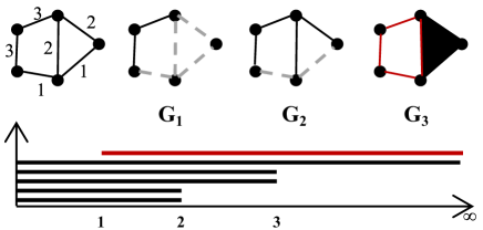
Topological Optimization. To introduce topological loss into the deep learning framework, we need to calculate its gradient. Computation of persistence homology is typically based on non-continuous matrix reduction algorithms. Since the output is in the form of a multiset, calculating the gradient directly poses difficulties. Following (Gabrielsson et al. 2020), given a graph filtration, each birth-death pair in persistence diagrams can be mapped to the edges that respectively created and destroyed the homology class. If the ordering on simplices is strict, the map will be unique, and we can obtain the gradient by inverse mapping the birth-death values to edge weights. Note that if the ordering is not strict, which is more likely, we can still extend the total order to a strict order either deterministically or randomly.

Experiments and Results

In this section, experiments on both synthetic data and real-world datasets are conducted to evaluate the performance and effectiveness of our algorithm. We compare the performance of our algorithm with the state-of-the-art algorithms. The experiment is repeated five times and the average results are reported to account for any variation in results.

Figure 6: Visualization of the demo graphs with their embedding and community topology. These three lines show graph, embedding, and community topology respectively. Different markers and colors represent different real clusters. The triangle in $(e)$ represents a 2-simplex and the red lines highlight a $\beta_{1}$

Experiments on Synthetic Data

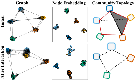
We reproduce a similar scenario in Fig.1: there are five groups of people, and two of them have additional links due to an ephemeral collaboration. We will show that TopoReg successfully ensures the temporal structure consistency of the community detection results. In Fig.6, a Gaussian random partition graph is initialized by creating 5 clusters each with a size drawn from a normal distribution $\mathcal{N}(20,1)$. Nodes are connected within clusters with a probability of 0.5 and between clusters with a probability of 0.001. Then, the other graph is created by randomly adding moderate amount of edges between 2 of the 5 clusters. Their node embeddings are visualized in the middle column respectively by dimension reduction to 2D via t-distributed stochastic neighbor embedding (t-SNE) (Van der Maaten and Hinton 2008). The third column shows that the collaboration leads to a sudden change in the community topology. Specifically, two 2-cliques are wiped out. The initial graph has 4 $\beta_{0}$ and 2 $\beta_{1}$ features, whereas the graph after interaction has only 3 $\beta_{0}$ and no $\beta_{1}$, since 2-simplex does not exist.

In such a situation, our algorithm is shown to have a binding influence on the node embedding, thus changing the clustering results and maintaining a stable topology between communities. We cluster the two graphs separately and optimize the clustering result of the second graph with $\mathcal{L}_{topo}$. In Fig. S1 (Appendix), we track the changes in node embedding, topological loss, and clustering effect. We find that the two clusters of points, which were initially more concentrated, gradually separate as the loss decreases. The clustering accuracy also improves from 81% to 98%.

Experiments on Real-world Datasets

Datasets We collected and processed four labeled dynamic network datasets without node features, including Enron, Highschool (Crawford and Milenković 2018), DBLP, Cora (Hou et al. 2020). Noting that each node in these existing datasets has a fixed label, we processed a new dataset DBLP_dyn from the original data, recalculating the node’s label at each snapshot. The brief information of these datasets is summarized in Table S1.

Figure 7: A comparison of node embeddings before and after applying TopoReg to GEC algorithm. The data is obtained from a single snapshot in the Highschool dataset, and the colors indicate the ground truth of community labels.

Data	Metrics	Static Baselines			Temporal Baselines			Ablation Study			Ours
		GEC	DAEGC	SDCN	DECS	ESPRA	DynAE	MFC	GEC+Topo	DAEGC+Topo	MFC+Topo
Enron	ACC	58.66	58.15	57.86	57.24	59.82	58.49	58.44	60.32	58.33	59.31
	NMI	15.42	15.69	12.44	15.63	13.85	7.10	18.9	18.14	17.53	19.14
	ARI	0.47	-0.81	-1.10	-1.90	-0.30	1.47	2.17	1.00	-0.36	2.73
	Modularity	30.42	30.08	-1.84	45.40	-2.10	-1.47	45.54	39.34	39.18	46.36
Highschool	ACC	49.21	49.33	24.02	65.77	26.44	18.82	68.91	63.51	62.66	70.67
	NMI	28.11	42.58	9.71	62.36	12.31	5.64	63.14	59.41	56.22	65.78
	ARI	13.57	26.43	0.46	36.18	0.12	0.11	48.77	44.44	38.93	50.87
	Modularity	49.82	56.35	-0.25	72.80	-0.95	-0.11	76.99	73.62	68.37	77.87
DBLP	ACC	56.38	56.23	56.22	OOM	OOM	68.31	56.83	57.62	56.54	57.98
	NMI	1.75	2.41	1.57	OOM	OOM	0.28	6.32	6.31	3.92	7.97
	ARI	0.25	0.35	0.37	OOM	OOM	0.05	0.98	1.37	0.62	1.41
	Modularity	56.07	59.28	4.54	OOM	OOM	0.07	85.39	76.71	71.61	86.65
Cora	ACC	35.18	37.56	34.17	OOM	OOM	37.85	50.66	43.18	41.6	52.53
	NMI	3.21	6.79	1.45	OOM	OOM	0.24	24.27	16.10	11.66	27.52
	ARI	1.18	3.05	0	OOM	OOM	0.18	13.49	8.04	5.50	14.62
	Modularity	47.70	49.94	3.59	OOM	OOM	1.32	74.09	63.05	55.53	75.61

Table 1: Experimental results on four datasets with known cluster numbers. $K$-means clustering is performed on graph embedding to obtain the final community membership. OOM means out-of memory.

Baselines

• Static Baselines. We first compare with state-of-the-art deep graph clustering method focusing on static community detection. DAEGC (Wang et al. 2019) first introduces the clustering module in DEC (Xie, Girshick, and Farhadi 2016) into the graph clustering problem. In order to simplify the problem and make the comparison fair, we also compare with the version that replaces GAT back to basic GCN in encoder, leaving other parts unchanged, which is called Graph Embedding Clustering (GEC). SDCN (Bo et al. 2020) improves deep clustering by integrating the structual information into representation learning module, but the core clustering module remain the same.

• Temporal Baselines. ESPRA (Wang, Gao, and Ma 2017), DECS (Liu et al. 2020) are two local smoothing dynamic community detection methods. Since they solve a multi-objective optimization problem with graph data in the form of a 3D matrix, they are too time- and memory-consuming and cannot be run on DBLP and Cora datasets. DynAE, DynRNN, DynAERNN (Goyal, Chhetri, and Canedo 2020) are a family of dynamic graph embedding algorithms that use recurrent neural networks to model temporal information in dynamic networks. DynRNN, DynAERNN expand network parameters based on DynAE. Limited by GPU memory, we only report DynAE results. Note that DECS is a label propagation algorithm and cannot fix the number of clusters, so we take the top $k-1$ clusters in the clustering result and merge the remaining nodes into one cluster.

Metrics We use Accuracy (ACC), Normalized Mutual Information (NMI), Adjusted Rand Index (ARI) to reflect how well the clustering results match the ground truth labels, and Modularity to reflect the clustering quality. All metrics are calculated at each snapshot and the average values are reported in Table 1.

Experimental Settings The experiments in this paper follow the following settings: node embedding dimension is 30, the learning rate is 0.001. Each backbone method uses one GNN layer (GCN, GAT). The other baseline models are set as default by the authors. The training is divided into two stages, $\alpha=10$, $\beta=0$ when training the backbone model and $\alpha=1$, $\beta=10$ when training the TopoReg, 500 epochs of each to ensure convergence. All weights in neural networks are initialized with Glorot initialization (Glorot and Bengio 2010).

Note that the nodes and edges in our dataset may appear and disappear in each snapshot, so the number of nodes per snapshot is not consistent. For temporal baselines that require a fixed-size dynamic adjacency matrix input, we add the points that do not appear in the current snapshot as isolated nodes. And to be fair, we remove these isolated nodes when calculating the metrics.

Figure 8: Comparisons of the Wasserstein distances between the community topology under the ground truth labels and the deep clustering labels before and after applying TopoReg.

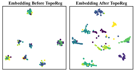
Results with Fixed Community Number Table 1 shows the experimental results on four real-world datasets with constant node labels. In such a situation, we assume that the community number $k$ is known and fixed, so $k$-means clustering is performed on each learned embedding. Topologically optimized MFC consistently achieves the best (bold) or second-best (underlined) accuracy, which demonstrates the superiority of our methodology. In addition, the TopoReg has an average improvement of 11.54%, 5.90%, and 1.38% on the three backbone models GEC, DAEGC, and MFC, respectively. Fig. 7 is a t-SNE visualization of node embedding on one snapshot in Highschool dataset before and after applying TopoReg to DEC. It is shown that the embedding gets scattered because TopoReg optimizes the problem of representation collapse by smoothing inter-community structure.

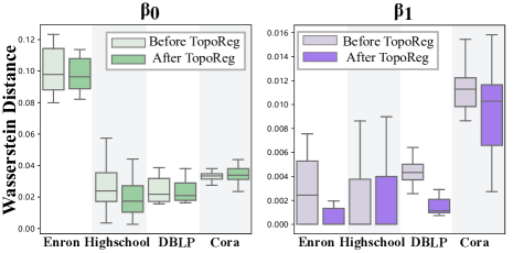
Meanwhile, to prove that we get a more stable community structure after using TopoReg, we computed the Wasserstein distance between the persistence diagrams of deep clustering results and that of the ground truth communities. The distribution of the distances are shown in Fig. 8. It can be seen that the topological consistency improvement of different datasets are reflected in different ways, including a decrease in median or variance. The enhancement tends to focus on $\beta_{0}$ or $\beta_{1}$ based on network properties. Overall, the inter-community structure after TopoReg is much closer to the one in the ground truth. The consistency of the ground truth labels suggests that we have found a more stable dynamic community detection results.

Results with Varying Community Number Table 2 shows the results on DBLP_dyn dataset. The true number of communities is not known in most cases. To solve that, a heuristic algorithm is often used to select the correct number of clusters, such as the elbow method (Liu and Deng 2020). When we set the clustering dimension $K$ to a relatively large value in the model and get the clustering result based on $\arg\max Q$. The number of clusters obtained will follow the clustering structure, and finally we get a detection result where the number of communities varies dynamically. For DEC-based backbone models, they are not as well adapted to TopoReg as our MFC in this situation.

Data	Metrics	GECQ+Topo	DAEGCQ+Topo	MFCQ+Topo
DBLPdyn	ACC	39.49	39.06	42.82
	NMI	2.91	2.13	9.32
	ARI	0.75	-3.61	2.68
	Modularity	61.27	34.83	84.71

Table 2: Experimental results on dataset with unknown cluster number. The label of the corresponding node is assigned as the index of the row maximum in cluster assignment distribution matrix.

Conclusion

This work proposes an end-to-end framework for dynamic community detection. It uses a neural network module MFC to implement matrix factorization for clustering, which outperforms the widely used self-supervised clustering method in the absence of node features. Regularization module TopoReg optimizes the cluster assignment distribution in deep graph clustering based on the topology of nearby snapshots. We demonstrate through synthetic and real dataset experiments that TopoReg can improve dynamic graph clustering results and preserve persistent community structure in terms of its topological features. It has good theoretical interpretability and can be easily extended to other depth graph clustering architectures. The two modules provide a trade-off between node clustering and topological stability of the community. Compared to other DEC-based backbone models such as DAEGC, TopoReg combines better with MFC in the case of unknown number of communities. At this point, we can obtain dynamically changing number of clusters based on the cluster assignment distribution learned. Using distributed computing and scalable graph representations like FastGAE (Salha et al. 2021), our method could be efficiently extended to large-scale graphs, since topological regularization is not directly affected by the size of graph, but only by the number of clusters.

References

- Blondel et al. (2008) Blondel, V. D.; Guillaume, J.-L.; Lambiotte, R.; and Lefebvre, E. 2008. Fast unfolding of communities in large networks. Journal of Statistical Mechanics: Theory and Experiment, 2008(10): P10008.
- Bo et al. (2020) Bo, D.; Wang, X.; Shi, C.; Zhu, M.; Lu, E.; and Cui, P. 2020. Structural deep clustering network. In Proceedings of The Web Conference 2020, 1400–1410.
- Boyd et al. (2011) Boyd, S.; Parikh, N.; Chu, E.; Peleato, B.; Eckstein, J.; et al. 2011. Distributed optimization and statistical learning via the alternating direction method of multipliers. Foundations and Trends® in Machine learning, 3(1): 1–122.
- Carlsson (2009) Carlsson, G. 2009. Topology and data. Bulletin of the American Mathematical Society, 46(2): 255–308.
- Carriere, Cuturi, and Oudot (2017) Carriere, M.; Cuturi, M.; and Oudot, S. 2017. Sliced Wasserstein kernel for persistence diagrams. In International conference on machine learning, 664–673. PMLR.
- Corne, Handl, and Knowles (2010) Corne, D.; Handl, J.; and Knowles, J. 2010. Evolutionary Clustering, 332–337. Boston, MA: Springer US. ISBN 978-0-387-30164-8.
- Crawford and Milenković (2018) Crawford, J.; and Milenković, T. 2018. ClueNet: Clustering a temporal network based on topological similarity rather than denseness. PloS One, 13(5): e0195993.
- Creswell et al. (2018) Creswell, A.; White, T.; Dumoulin, V.; Arulkumaran, K.; Sengupta, B.; and Bharath, A. A. 2018. Generative adversarial networks: an overview. IEEE Signal Processing Magazine, 35(1): 53–65.
- Dey and Wang (2022) Dey, T. K.; and Wang, Y. 2022. Computational topology for data analysis. Cambridge University Press.
- Du et al. (2023) Du, K.-L.; Swamy, M. N. S.; Wang, Z.-Q.; and Mow, W. H. 2023. Matrix Factorization Techniques in Machine Learning, Signal Processing, and Statistics. Mathematics, 11(12).
- Gabrielsson et al. (2020) Gabrielsson, R. B.; Nelson, B. J.; Dwaraknath, A.; and Skraba, P. 2020. A topology layer for machine learning. In International Conference on Artificial Intelligence and Statistics, 1553–1563. PMLR.
- Glorot and Bengio (2010) Glorot, X.; and Bengio, Y. 2010. Understanding the difficulty of training deep feedforward neural networks. In Teh, Y. W.; and Titterington, M., eds., Proceedings of the Thirteenth International Conference on Artificial Intelligence and Statistics, volume 9 of Proceedings of Machine Learning Research, 249–256. Chia Laguna Resort, Sardinia, Italy: PMLR.
- Goyal, Chhetri, and Canedo (2020) Goyal, P.; Chhetri, S. R.; and Canedo, A. 2020. dyngraph2vec: Capturing network dynamics using dynamic graph representation learning. Knowledge-Based Systems, 187: 104816.
- Guo and Lyu (2004) Guo, P.; and Lyu, M. R. 2004. A pseudoinverse learning algorithm for feedforward neural networks with stacked generalization applications to software reliability growth data. Neurocomputing, 56: 101–121.
- Guo et al. (2017) Guo, X.; Gao, L.; Liu, X.; and Yin, J. 2017. Improved Deep Embedded Clustering with Local Structure Preservation. In Proceedings of the 26th International Joint Conference on Artificial Intelligence, IJCAI’17, 1753–1759. AAAI Press. ISBN 9780999241103.
- Hajij et al. (2018) Hajij, M.; Wang, B.; Scheidegger, C.; and Rosen, P. 2018. Visual Detection of Structural Changes in Time-Varying Graphs Using Persistent Homology. In 2018 IEEE Pacific Visualization Symposium (PacificVis), 125–134.
- Hou et al. (2020) Hou, C.; Zhang, H.; He, S.; and Tang, K. 2020. Glodyne: Global topology preserving dynamic network embedding. IEEE Transactions on Knowledge and Data Engineering, 34(10): 4826–4837.
- Huang and Ribeiro (2016) Huang, W.; and Ribeiro, A. 2016. Persistent homology lower bounds on high-order network distances. IEEE Transactions on Signal Processing, 65(2): 319–334.
- Javed et al. (2018) Javed, M. A.; Younis, M. S.; Latif, S.; Qadir, J.; and Baig, A. 2018. Community detection in networks: A multidisciplinary review. Journal of Network and Computer Applications, 108: 87–111.
- Kipf and Welling (2016) Kipf, T. N.; and Welling, M. 2016. Variational Graph Auto-Encoders. stat, 1050: 21.
- Liu and Deng (2020) Liu, F.; and Deng, Y. 2020. Determine the number of unknown targets in open world based on elbow method. IEEE Transactions on Fuzzy Systems, 29(5): 986–995.
- Liu et al. (2020) Liu, F.; Wu, J.; Xue, S.; Zhou, C.; Yang, J.; and Sheng, Q. 2020. Detecting the evolving community structure in dynamic social networks. World Wide Web, 23: 715–733.
- Liu et al. (2023) Liu, M.; Liu, Y.; Liang, K.; Wang, S.; Zhou, S.; and Liu, X. 2023. Deep Temporal Graph Clustering. arXiv:2305.10738.
- Liu et al. (2013) Liu, M.-Y.; Tuzel, O.; Ramalingam, S.; and Chellappa, R. 2013. Entropy-rate clustering: Cluster analysis via maximizing a submodular function subject to a matroid constraint. IEEE Transactions on Pattern Analysis and Machine Intelligence, 36(1): 99–112.
- Liu et al. (2022) Liu, Y.; Tu, W.; Zhou, S.; Liu, X.; Song, L.; Yang, X.; and Zhu, E. 2022. Deep graph clustering via dual correlation reduction. In Proceedings of the AAAI Conference on Artificial Intelligence, volume 36, 7603–7611.
- Lozeve (2018) Lozeve, D. 2018. Topological Data Analysis of Temporal Networks. Ph.D. thesis, University of Oxford.
- Ng, Jordan, and Weiss (2001) Ng, A. Y.; Jordan, M. I.; and Weiss, Y. 2001. On Spectral Clustering: Analysis and an Algorithm. In Proceedings of the 14th International Conference on Neural Information Processing Systems: Natural and Synthetic, NIPS’01, 849–856. Cambridge, MA, USA: MIT Press.
- Pareja et al. (2020) Pareja, A.; Domeniconi, G.; Chen, J.; Ma, T.; Suzumura, T.; Kanezashi, H.; Kaler, T.; Schardl, T. B.; and Leiserson, C. E. 2020. EvolveGCN: Evolving graph convolutional networks for dynamic graphs. In AAAI Conference on Artificial Intelligence. AAAI press.
- Park et al. (2022) Park, N.; Rossi, R.; Koh, E.; Burhanuddin, I. A.; Kim, S.; Du, F.; Ahmed, N.; and Faloutsos, C. 2022. Cgc: Contrastive graph clustering forcommunity detection and tracking. In Proceedings of the ACM Web Conference 2022, 1115–1126.
- Peng et al. (2021) Peng, Z.; Liu, H.; Jia, Y.; and Hou, J. 2021. Attention-driven graph clustering network. In Proceedings of the 29th ACM International Conference on Multimedia, 935–943.
- Petri et al. (2013) Petri, G.; Scolamiero, M.; Donato, I.; and Vaccarino, F. 2013. Topological strata of weighted complex networks. PloS One, 8(6): e66506.
- Rieck et al. (2017) Rieck, B.; Fugacci, U.; Lukasczyk, J.; and Leitte, H. 2017. Clique community persistence: A topological visual analysis approach for complex networks. IEEE Transactions on Visualization and Computer Graphics, 24(1): 822–831.
- Salehi and Davulcu (2020) Salehi, A.; and Davulcu, H. 2020. Graph attention auto-Encoders. In 2020 IEEE 32nd International Conference on Tools with Artificial Intelligence (ICTAI), 989–996. IEEE Computer Society.
- Salha et al. (2021) Salha, G.; Hennequin, R.; Remy, J.-B.; Moussallam, M.; and Vazirgiannis, M. 2021. FastGAE: Scalable Graph Autoencoders with Stochastic Subgraph Decoding. Neural Netw., 142(C): 1–19.
- Songdechakraiwut and Chung (2023) Songdechakraiwut, T.; and Chung, M. K. 2023. Topological learning for brain networks. The Annals of Applied Statistics, 17(1): 403.
- Su et al. (2022) Su, X.; Xue, S.; Liu, F.; Wu, J.; Yang, J.; Zhou, C.; Hu, W.; Paris, C.; Nepal, S.; Jin, D.; et al. 2022. A comprehensive survey on community detection with deep learning. IEEE Transactions on Neural Networks and Learning Systems.
- Van der Maaten and Hinton (2008) Van der Maaten, L.; and Hinton, G. 2008. Visualizing data using t-SNE. Journal of Machine Learning Research, 9(11).
- Wang et al. (2019) Wang, C.; Pan, S.; Hu, R.; Long, G.; Jiang, J.; and Zhang, C. 2019. Attributed graph clustering: A deep attentional embedding approach. arXiv preprint arXiv:1906.06532.
- Wang, Gao, and Ma (2017) Wang, P.; Gao, L.; and Ma, X. 2017. Dynamic community detection based on network structural perturbation and topological similarity. Journal of Statistical Mechanics: Theory and Experiment, 2017(1): 013401.
- Xie, Girshick, and Farhadi (2016) Xie, J.; Girshick, R.; and Farhadi, A. 2016. Unsupervised deep embedding for clustering analysis. In International conference on machine learning, 478–487. PMLR.
- Yan et al. (2021) Yan, Z.; Ma, T.; Gao, L.; Tang, Z.; and Chen, C. 2021. Link prediction with persistent homology: An interactive view. In International Conference on Machine Learning, 11659–11669. PMLR.
- You et al. (2021) You, J.; Hu, C.; Kamigaito, H.; Funakoshi, K.; and Okumura, M. 2021. Robust dynamic clustering for temporal networks. In Proceedings of the 30th ACM International Conference on Information & Knowledge Management, 2424–2433.
- Zhang et al. (2022) Zhang, H.; Li, P.; Zhang, R.; and Li, X. 2022. Embedding graph auto-encoder for graph clustering. IEEE Transactions on Neural Networks and Learning Systems.
- Zhang et al. (2019) Zhang, S.; Tong, H.; Xu, J.; and Maciejewski, R. 2019. Graph convolutional networks: a comprehensive review. Computational Social Networks, 6(1): 1–23.
- Zhou et al. (2022) Zhou, S.; Xu, H.; Zheng, Z.; Chen, J.; Bu, J.; Wu, J.; Wang, X.; Zhu, W.; Ester, M.; et al. 2022. A comprehensive survey on deep clustering: Taxonomy, challenges, and future directions. arXiv preprint arXiv:2206.07579.
- Zhou, Lü, and Zhang (2009) Zhou, T.; Lü, L.; and Zhang, Y.-C. 2009. Predicting missing links via local information. The European Physical Journal B, 71(4): 623–630.